| Issue |
A&A
Volume 616, August 2018
|
|
|---|---|---|
| Article Number | A151 | |
| Number of page(s) | 14 | |
| Section | Planets and planetary systems | |
| DOI | https://doi.org/10.1051/0004-6361/201832963 | |
| Published online | 07 September 2018 | |
Na I and Hα absorption features in the atmosphere of MASCARA-2b/KELT-20b⋆
1
Instituto de Astrofísica de Canarias, Vía Láctea s/n, 38205 La Laguna, Tenerife, Spain
e-mail: This email address is being protected from spambots. You need JavaScript enabled to view it.
2
Departamento de Astrofísica, Universidad de La Laguna, Spain
3
Max Planck Institute for Astronomy, Königstuhl 17, 69117 Heidelberg, Germany
4
Key Laboratory of Planetary Sciences, Purple Mountain Observatory, Chinese Academy of Sciences, Nanjing 210008, PR China
5
Stellar Astrophysics Centre, Department of Physics and Astronomy, Aarhus University, Ny Munkegade 120, 8000 Aarhus C, Denmark
6
Leiden Observatory, Leiden University, Postbus 9513, 2300 RA Leiden, The Netherlands
7
Consejo Superior de Investigaciones Científicas, Spain
Received:
6
March
2018
Accepted:
7
May
2018
Abstract
We used the HARPS-North high resolution spectrograph (ℛ = 115 000) at Telescopio Nazionale Galileo (TNG) to observe one transit of the highly irradiated planet MASCARA-2b/KELT-20b. Using only one transit observation, we are able to clearly resolve the spectral features of the atomic sodium (Na I) doublet and the Hα line in its atmosphere, which are corroborated with the transmission calculated from their respective transmission light curves (TLC). In particular, we resolve two spectral features centered on the Na I doublet position with an averaged absorption depth of 0.17 ± 0.03% for a 0.75 Å bandwidth with line contrasts of 0.44 ± 0.11% (D2) and 0.37 ± 0.08% (D1). The Na I TLC have also been computed, showing a large Rossiter-McLaughlin (RM) effect, which has a 0.20 ± 0.05% Na I transit absorption for a 0.75 Å passband that is consistent with the absorption depth value measured from the final transmission spectrum. We observe a second feature centered on the Hα line with 0.6 ± 0.1% contrast and an absorption depth of 0.59 ± 0.08% for a 0.75 Å passband that has consistent absorptions in its TLC, which corresponds to an effective radius of Rλ/RP = 1.20 ± 0.04. While the signal-to-noise ratio (S/N) of the final transmission spectrum is not sufficient to adjust different temperature profiles to the lines, we find that higher temperatures than the equilibrium (Teq = 2260 ± 50 K) are needed to explain the lines contrast. Particularly, we find that the Na I lines core require a temperature of T = 4210 ± 180 K and that Hα requires a temperature of T = 4330 ± 520 K. MASCARA-2b, like other planets orbiting A-type stars, receives a large amount of UV energy from its host star. This energy excites the atomic hydrogen and produces Hα absorption, leading to the expansion and abrasion of the atmosphere. The study of other Balmer lines in the transmission spectrum would allow the determination of the atmospheric temperature profile and the calculation of the lifetime of the atmosphere with escape rate measurements. In the case of MASCARA-2b, residual features are observed in the Hβ and Hγ lines, but they are not statistically significant. More transit observations are needed to confirm our findings in Na I and Hα and to build up enough S/N to explore the presence of Hβ and Hγ planetary absorptions.
Key words: planetary systems / techniques: spectroscopic / planets and satellites: atmospheres / methods: observational / planets and satellites: individual: MASCARA-2b / planets and satellites: individual: KELT-20b
The reduced HARPS spectra are only available at the CDS via anonymous ftp to cdsarc.u-strasbg.fr (130.79.128.5) or via http://cdsweb.u-strasbg.fr/cgi-bin/qcat?J/A+A/616/A151
© ESO 2018
1. Introduction
After the first detection of an exoplanet atmosphere by Charbonneau et al. (2002), which revealed the presence of atomic sodium (Na I) thanks to space-based instruments, several studies have been carried out using ground-based facilities. These facilities have been slowly overcoming the limitations imposed by the telluric atmospheric variations, resulting in detections of spectral signatures arising from Rayleigh scattering, i.e., Na and K with low spectral resolution spectrographs (e.g., Sing et al. 2012; Murgas et al. 2014; Wilson et al. 2015; Nortmann et al. 2016; Chen et al. 2017; Palle et al. 2017). Observations with high resolution spectrographs are able to deal with the remaining limitations due to the telluric atmosphere by resolving the spectral lines and taking advantage of the various Doppler velocities of the Earth, host star, and exoplanet.
One of the most studied species in the upper atmosphere of hot exoplanets is the Na I doublet (D2 at λ5889.951 Å and D1 at λ5895.924 Å) as a consequence of its high cross section. The first ground-based detection of Na I was performed by Redfield et al. (2008) using the High Resolution Spectrograph (HRS), with ℛ = λ/∆λ ∼ 60 000, mounted on the 9.2 m Hobby-Eberly Telescope. Shortly after, Snellen et al. (2008) confirmed the Na I in HD 209458b atmosphere using the High Dispersion Spectrograph (HDS), with ℛ ∼ 45 000, on the 8 m Subaru Telescope. Recently, ground-based studies with the High Accuracy Radial velocity Planet Searcher (HARPS) spectrograph (ℛ ∼ 115 000), at ESO 3.6 m telescope in la Silla (Chile) and at 3.58 m Telescopio Nazionale Galileo (TNG) in Roque de los Muchachos Observatory (ORM, la Palma), have been able to resolve the individual Na I line profiles of HD 189733b (Wyttenbach et al. 2015), WASP-49b (Wyttenbach et al. 2017), and WASP-69b (Casasayas-Barris et al. 2017). Using these same data sets Heng et al. (2015) were able to study the existence of temperature gradients, Louden & Wheatley (2015) explored the high-altitude winds of HD 189733b, Barnes et al. (2016) studied stellar activity signals, and Yan et al. (2017) analyzed the center-to-limb variation (CLV) effect in the transmission light curve (TLC) of this exoplanet. In the near future, high-dispersion methods will be very important in the observations of spectral features of temperate rocky planets and super-Earths; these features will be out of reach of the James Webb Space Telescope (JWST), but available with the upcoming facilities such as ESPRESSO on the Very Large Telescope (VLT) or HIRES on E-ELT (Snellen et al. 2013; Lovis et al. 2017).
We present the results from only one transit observation of MASCARA-2b, obtained with the HARPS-North spectrograph (la Palma). MASCARA-2b (Talens et al. 2018; Lund et al. 2017) is a hot Jupiter (RP = 1.83 ± 0.07 RJup, MP ˂ 3.510 MJup) transiting a rapidly rotating (v sin i⋆ = 115.9 ± 3.4 km s−1) A2-type star with an orbital period of  days (see Table 1 for details). This star, MASCARA-2 (also named KELT-20 or HD 185603), is the fourth brightest star (mv = 7.6) with a transiting planet known to date. With the combination of the early spectral type, the brightness, and the rapid rotation of its host star, MASCARA-2b is an ideal target for transmission spectroscopy.
MASCARA-2b is one of the few exoplanets transiting an A-type star known to date with effective temperatures higher than ∼7000 K. These planets typically receive a large amount of extreme ultraviolet radiation from its host star, exciting the atomic hydrogen to produce Hα absorption and leading to the expansion and possibly abrasion of their atmosphere (Bourrier et al. 2016). The study of the Balmer lines of these planets allows us to estimate the lifetime of the atmosphere from the escape rate measurement. Comparative studies of this planet population, which present different system properties, will help us to understand their origin and evolution.
Physical and orbital parameters of MASCARA-2b.
2. Observations
We observed one transit of MASCARA-2b on 16 August 2017 using the HARPS-North spectrograph mounted on the 3.58 m TNG, located at the Observatorio del Roque de los Muchachos (ORM, La Palma). For this transit, the observations started at 21:21 UT and finished at 03:56 UT, with an airmass variation from 1.0 to 2.1.
The observations were carried out exposing continuously before, during, and after the transit to retrieve a good baseline, which is key for the data reduction process. We used fiber A on the target and fiber B on the sky to correct possible emission features from the Earth’s atmosphere. Since MASCARA-2 is a bright star, with a magnitude of 7.6 (V), we exposed 200 s per exposure, recording a total of 90 consecutive spectra; 58 of these were recorded during the transit. The individual retrieved spectra have a signal-to-noise ratio (S/N) ranging from 40 to 80 per wavelength bin in the continuum near the Na I doublet. One spectrum of the rapid-rotator telluric standard HR 7390 (5.59 V) was also observed before MASCARA-2b observations, using 300 s of exposure time, with an airmass of 1.0, and obtaining a S/N of ∼170 in the continuum. HR 7390 is a bright A0V-type star that has a projected rotation speed of 150 km s−1.
3. Methods
The observations were reduced with the HARPS-North Data reduction Software (DRS), version 1.1. The DRS extracts the spectra order-by-order, and these spectra are then flat-fielded using the daily calibration set. A blaze correction and the wavelength calibration are applied to each spectral order and, finally, all the spectral orders from each two-dimensional echelle spectrum are combined and resampled into a one-dimensional spectrum ensuring flux conservation. The resulting one-dimensional spectra covers a wavelength range between 3800 Å and 6900 Å and has a wavelength step of 0.01 Å, referred to the solar system barycenter rest frame and in air wavelengths. One representative spectrum of MASCARA-2 and the telluric standard HR 7390 are presented in Fig. 1.
The first step of our analysis is the telluric contamination subtraction. Near the Na I doublet, the main telluric contributors are water and telluric sodium (Snellen et al. 2008). Each individual target sky spectrum was examined to look for the presence of telluric sodium, but no sodium emission was observed. For an A-type star as MASCARA-2, the method used in Casasayas-Barris et al. (2017) to remove the telluric features produced by water and oxygen does not work as well as for other spectral types. Thus, we correct for this contamination using a combination of the methods of Wyttenbach et al. (2015) and Casasayas-Barris et al. (2017), taking advantage of the observations of the telluric standard HR 7390. With the method described in Astudillo-Defru & Rojo (2013), which makes the assumption that the variation of the telluric lines follows linearly the airmass variation, we computed a high-quality telluric spectrum. The difference is that, before computing the high-quality telluric spectrum, we aligned all the telluric lines via Barycentric Earth Radial Velocity (BERV) information from the HARPS-N file headers. Then, instead of scaling all the MASCARA-2 spectra to the averaged in-transit airmass as in Wyttenbach et al. (2015), we scaled them to the telluric standard airmass (i.e., 1.0 in this case). Finally, and after removing the small stellar features from the telluric standard spectrum as in Frasca et al. (2000), we divided each scaled MASCARA-2 spectrum by the final telluric standard spectrum, which has been also shifted to the Earth’s reference frame.
Once the telluric contamination has been removed, we followed the steps described in Casasayas-Barris et al. (2017) to extract the transmission spectrum of the planet. We note that the stellar radial velocity (RV) information of MASCARA-2, as for other rapidly rotating A-type stars, is not well determined by the HARPS-N pipeline. For rapidly rotating early-type stars, which present very broad lines in their spectrum, the stellar RV correction is not very important and the possible uncorrected RV shift between the spectra does not result in a large difference. Therefore, we do not consider the stellar RV correction here. However, if the stellar lines are deep and narrow, the RV correction becomes important. In this way, the possible instrumental RV effects are not considered, but such effects produce offsets that similarly affect all spectra, resulting in a global wavelength shift with respect the expected rest-frame position.
The combination of all the out-of-transit spectra (master out) after subtracting the telluric contamination is shown in Fig. 1. Sharp residuals can be observed at ∼5890 Å and at ∼5896 Å (less deeper), which appear in each in-transit and out-of-transit spectra. The measured RV of both signals is −14.9 ± 0.5 km s−1 and there is no wavelength shift during the observation. In order to determine their origin, we used the LISM Kinematic Calculator (Redfield & Linsky 2008), which gives us information about the interstellar medium clouds that our line-of-sight traverses while observing a target. In the case of MASCARA-2b, according to the interstellar medium distribution in our Galaxy, the sight line went through the G, Mic and Oph clouds, which have −14.10 ± 0.97 km s−1, −20.90 ± 1.34 km s−1, −28.31 ± 0.93 km s−1 RVs, respectively. The very similar RV of the G cloud and the residuals observed in the data is the evidence of their possible interstellar origin. Since the interstellar sodium does not show any shift during the night and, in this particular case, we are not correcting for the stellar RV, the presence of interstellar species is not a problem, as it is compensated when dividing the in-transit spectra by the master out spectrum.
During the observation, the planet is moving along the orbit, changing its RV with respect to the observer. This RV change results in a wavelength shift of the measured planetary absorption lines that needs to be corrected. When the in-transit spectra are divided by the master out spectrum, each of these spectra contain residuals that need to be shifted to the planetary rest frame to become aligned before being co-added. In this work, this wavelength shift is obtained by calculating the theoretical RV of the planet along the orbit and projecting it to the line of sight of the observer. MASCARA-2b is a recently discovered planet and only an upper limit of its mass (∼3.5 MJup; Lund et al. 2017) is known. For this reason, to calculate the RV we consider that MP ˝ M⋆ (i.e., assuming the planetary mass does not significantly contribute to the reduced mass of the system). The calculated RV changes during the transit from −24 km s−1 to +24 km s−1, approximately. The maximum difference of this RV between considering the mass upper limit and the MP ˝ M⋆ approximation is ∼±0.1 km s−1, which is not significant considering that a pixel in HARPS-N corresponds to ∼0.8 km s−1.
Finally, we model the stellar spectrum for different orbital phases of the planet using ATLAS9 models (Heiter et al. 2002). The modeled spectra contain both the CLV and Rossiter-McLaughlin (RM) effects on the stellar lines shape (see top panel of Fig. 2). The CLV effect is obtained by computing the stellar spectra with various µ angles as in Yan et al. (2015) and the RM effect is obtained assuming rigid rotation with a spin-orbit angle of 0◦ (Talens et al. 2018 measured λ = 0.6 ± 4◦), stellar rotation of v sin i = 115 km s−1, and an impact parameter of 0.5 (Lund et al. 2017). By applying the same method to these synthetic spectra, we obtain how the RM and CLV affect the final transmission spectrum of the planet (see bottom panel of Fig. 2). As can be observed, although the expected RM effect is large, the combination of both effects is on the order of ∼10−4 (i.e., one magnitude below the typical noise). This is because the CLV is very weak for these spectral-type stars and the RM is smeared when the in-transit spectra are combined. Nevertheless, we divide the final transmission spectrum by the model to correct for these effects.
A kind of two-dimensional representation of the original spectra and the results after the different processing steps described in this section are presented in the Appendix A. In these figures, the RM effect on the lines and the exoplanet absorption in the stellar and planetary rest frame can be seen.
 |
Fig. 1. Normalized spectra of the telluric standard HR 7390 (blue) and MASCARA-2 (black) around the Na I region after their reduction with the HARPS DRS. In green we show the MASCARA-2 master out spectrum after the telluric correction. |
 |
Fig. 2. Modeled spectra of MASCARA-2 for various orbital phases of the planet using LTE and a spin-orbit angle of 0◦ (Talens et al. 2018) for the RM effect (top) and modeled RM and CLV effects in the final transmission spectrum (bottom). We note the large RM effect in the stellar lines. |
4. Results
4.1. Transmission spectrum analysis of Na I
The S/N per extracted pixel in the continuum near the Na I doublet for the observed spectra of MASCARA-2, retrieved with HARPS-N, ranges from 40 to 80. When combining the spectra to obtain the master spectrum for in-transit observations and out-of-transit observations the S/N increases to ∼150, and when co-adding all the spectra to compute the final transmission spectrum the S/N increases to ∼450.
The final transmission spectrum of MASCARA-2b around the Na I is shown in Fig. 3. As can be observed in this Figure, both Na I D lines show a peak relative to the continuum. With a Gaussian fit to each Na I line, we measure line contrasts of 0.44 ± 0.11% (D2) and 0.37 ± 0.08% (D1) and a full width at half maximum (FWHM) of 0.26 ± 0.08 Å (D2) and 0.33 ± 0.08 Å (D1), centered on 5889.93 ± 0.03 Å (D2) and 5895.88 ± 0.03 Å (D1). The expected values for the D2 and D1 lines in the planetary rest frames are 5889.95 Å and 5895.92 Å, respectively, implying that no net blueshift or redshift is measured. In both cases the Gaussian fit has a reduced χ2 value of ∼1.2. This fit procedure is performed using a simple Markov chain Monte Carlo (MCMC), and the best-fit values are obtained at 50% (median) and their error bars correspond to the 1σ statistical errors at the corresponding percentiles.
The absorption depth of the Na I lines is measured by calculating the weighted mean of the flux in a central passband of different bandwidths (0.188 Å, 0.375 Å, 0.75 Å, 1.5 Å, 3.0 Å, and 5.0 Å) centered on each Na I lines, and then compared with the average of two 12 Å bandwidths taken in the continuum of the transmission spectrum of the Na I lines: one in the blue (B = [5872.89 − 5884.89] Å) and one in the red (R = [5900.89 − 5912.89] Å) regions. The final values are presented in Table 2. We note that all the uncertainties are calculated with the error propagation of the photon noise level and the readout noise from the original data.
We performed various control distributions (not shown here) to ensure that the results are not caused by stellar or telluric residuals, but can only be obtained with the correct selection of the in- and out-of-transit samples. In particular, we computed the transmission spectrum by only considering the in-transit spectra, which were randomly selected to form the synthetic in- and out-of-transit samples. The same test was performed by considering only the out-of-transit files and also selecting the even files as the in-transit sample and the odd files as the out-of-transit sample. In all tests, the resulting synthetic transmission spectra are mainly flat and there is a clear difference between these spectra and the lines depth of the real transmission spectrum. The averaged absorption depth in the expected Na I D2 and D1 lines position for a 0.75 Å bandwidth are 0.021 ± 0.055%, 0.058 ± 0.040%, and 0.087 ± 0.032% for the out-out, in-in, and even-odd samples, respectively. The final transmission spectrum with a non-correction of the planet RV was also computed with no signals in the Na I position (0.045 ± 0.029% of absorption for a 0.75 Å bandwidth), supporting the theory that the possible interstellar sodium does not affect the final result and the Na I signals observed in the final transmission spectrum only appear in the planetary rest frame. In addition, this is evidence that we do not observe stellar activity signals, which would be visible in the stellar rest frame if they were present (Wyttenbach et al. 2017). As can be observed, the in-in and even-odd distributions absorption depths, the final transmission spectra are not totally flat as in the out-out sample. We note that in these distributions we do not correct for the CLV + RM effects and, as can be observed in the TLC, the in-transit absorption varies during the transit. These effects could introduce some variations in the absorption and not allow the total compensation of the planet absorption in the in-in and even-odd to control distributions. This does not happen in the out-out sample, as expected. On the other hand, the small absorption measured when the planet RV is not considered could be produced because the residuals partially overlap in the stellar rest frame.
As noted in Sect. 3, since no precise RV parameters have been measured for MASCARA-2b system, we tested the result with stellar RV corrected using the upper limit value of the RV semiamplitude (322.51 m s−1, Lund et al. 2017) and a theoretical RM effect model calculated using Ohta et al. (2005). The resulting transmission spectrum is very similar to the result without stellar RV correction (see Fig. 4). As no significant differences are observed in the measurements when the stellar RV is corrected and when it is not, we show our analysis based on the case in which the stellar RV is not contemplated as this is the most correct procedure in this particular case.
 |
Fig. 3. Transmission spectrum of MASCARA-2b atmosphere in the region of Na I D doublet. In the top panel the atmospheric transmission spectrum is presented in light gray. Black dots indicate the binned transmission spectrum by 10 pixels and the Gaussian fit to each Na I D lines is shown in red; its residuals are shown in the bottom panel. The expected wavelength position of the Na I doublet lines, in the planetary reference frame, are indicated with blue vertical lines. The uncertainties of the relative flux come from the error propagation of the photon and readout noise from the original data. |
Summary of the measured relative absorption depth in [%] in the Na I D lines of the final transmission spectrum and the TLC of MASCARA-2b for various bandwidths.
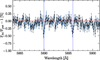 |
Fig. 4. Comparison between the transmission spectra obtained with (light blue line) and without (black line) stellar RV correction, before correcting for the final RM and CLV effects. In both cases the spectrum is binned by 10 pixels. The blue vertical lines show the expected wavelength position of the Na I D lines and the red horizontal line is the null-absorption reference. |
4.2. Transmission light curve of Na I
The transit light curve of the Na I D lines is calculated as presented in Yan et al. (2017) and Casasayas-Barris et al. (2017) using four different bandwidths: 0.75 Å, 1.5 Å, 3.0 Å, 5.0 Å. Since the stellar lines are broad because of the rapid-rotation of the star (v sin i⋆ = 115 km s−1) and we expect a large RM effect, we included the calculation for a broad 5.0 Å passband, which encompasses the full Na I line. As reference passbands we use the same wavelength regions presented in Sect. 4.1. The results of both D1 and D2 lines are averaged and, finally, the data are binned with a 0.003 phase step (∼3.3 km s−1 of planetary RV), taking into account the S/N of the data. The final observed light curves for the various bandwidths are shown in the first row of Fig. 5.
The resulting light curves are the combination of the planetary absorption, CLV, and RM effects. For MASCARA-2 we expect a large RM (see Fig. 2 and Lund et al. 2017) and a small CLV effect. We note that both effects produce similar shapes in the TLC (see Yan et al. 2017) because in this case the RM has the most significant contribution. It is noticeable how the RM effect in the TLC diminishes as the width of the central passband is increased. This is because the deformation in the stellar sodium lines due to the RM effect occurs during different phases of the transit and, for small bandwidths, it can move in and out of the reference passbands. However, the 5 Å passband encompasses the complete stellar sodium lines, averaging out the effect in the TLC.
To correct for these effects we divide the observed TLC by the light curve with the modeled effects (see second and third row of Fig. 5). We note that the modeled CLV + RM light curves are directly derived from the spectral models shown in Fig. 2, and the fitting procedure is only applied to the Na I absorption model. This fitting is performed using a simple MCMC algorithm and the model built with PyTransit (Parviainen 2015). This model depends on the orbital period (P), excentricity (e), planet-star ratio (RP/R⋆), scaled semimajor axis (a/R⋆), orbital inclination (i), transit center (T0), argument of periastron (ω) and quadratic limb darkening coefficients (u). The u coefficients are fixed to the estimated values calculated with the PyLDTk (Parviainen & Aigrain 2015) Python Package, which use the library of PHOENIX stellar atmospheres (Husser et al. 2013), Rp/R⋆ remains free and the other parameters are fixed to the values presented in Table 1.
As can be observed, the CLV + RM model is slightly underestimated compared to the measurements, which is possibly due to the assumption of local thermodynamical equilibrium (LTE) during the model computation (Yan et al. 2017). With the final Na I TLC it is possible to calculate the true absorption depth by comparing the weighted mean of the in-transit and out-of-transit values (see the results in Table 2). These values are consistent with the measured absorption depth values derived from the final transmission spectrum of MASCARA-2b; these findings are presented in the same table for a better comparison.
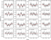 |
Fig. 5. Na I TLC from HARPS-N observations of MASCARA-2b for four bandwidths: 0.75 Å (first column), 1.5 Å (second column), 3.0 Å (third column), and 5.0 Å (fourth column). In all panels, the light gray dots indicate the values from all the spectra, and the black dots the same data binned with 0.003 phase step. First row: observed TLC of the Na I D lines from our data reduction. The relative flux of the D1 and D2 lines is averaged. The red line indicates the modeled TLC, which is the combination of the best-fit Na I absorption and the CLV and RM effects (Yan et al. 2017). This model is calculated theoretically and there is no fitting to the data. Second row: the CLV + RM effects. The black line indicates the result of removing the Na I absorption model from the observed TLC. The modeled CLV and RM effects are shown in red. Third row: the Na I absorption light curve obtained dividing the observed TLC by the modeled CLV + RM effects (black line). The red line is the best-fit Na I absorption model. Fourth row: residuals between the observed TLC and the model. We note the different y-scale of the panels. |
4.3. Analysis of Hα region
Following the same methods, we analyzed the region around the Hα line (λ6562.80 Å) in the MASCARA-2b spectrum; see the two-dimensional representation of the spectra in Appendix A. In the telluric correction, we subtract the sky spectrum to correct for possible telluric Hα emission. The Hα line observed in MASCARA-2 spectra is more than 50 Å (5000 pixels) broad, for this reason the transmission spectrum is binned by 30 pixels in this case (see Fig. 6) and larger bandwidths (3.0 Å, 5.0 Å, 10.0 Å, and 20.0 Å) are used to calculate the TLC (see Fig. 7), with 12.0 Å reference passbands at B = [6480.00 − 6492.00] Å and R = [6628.00 − 6640.00] Å.
A Gaussian feature with a contrast of 0.63 ± 0.09% and a FWHM of 0.95 ± 0.16 Å is observed in the Hα position (6562.74 ± 0.08 Å), and the measured absorption depth is 0.378 ± 0.056% for a 1.5 Å passband (more values are presented in Table 3). As for the Na I, the Hα TLC present a strong RM shape for small passbands that slowly disappears for larger bandwidths (see Fig. 7). This RM effect is compensated at about ∼50.0 Å central passbands when the stellar line is totally encompassed. However, in this case the possible Hα absorption is attenuated in the large passband and the transit light curve becomes flat. The Hα absorption depths measured in the TLC measured with different passbands, after correcting for the RM+CLV effect, are presented in Table 3. Similar to the case of Na I absorption, these values are in agreement with the measured absorption depth values from the final transmission spectrum, giving strong confidence in our results.
The same control distributions to those presented for Na I are performed for Hα. For a 0.75 Å bandwidth we measure absorption depths of 0.016 ± 0.141%, 0.075 ± 0.110%, 0.136 ± 0.085%, and 0.387 ± 0.078%, for the out-out, in-in, even-odd, and no planet RV samples, respectively. In this case, when the planet RV correction is not applied we measure a significant absorption depth. This is probably because Hα is a very broad line and the planetary signals partially overlap even if the planet RV is not corrected.
 |
Fig. 6. Transmission spectrum of MASCARA-2b atmosphere in the region of Hα. Top panel: atmospheric transmission spectrum (light gray) and binned transmission spectrum by 30 pixels (black dots). The Gaussian fit is shown in red. Bottom panel: residuals of the Gaussian fit. The blue vertical line indicates the expected wavelength position in the planetary reference frame. |
Summary of the measured relative absorption depth in [%] in the Hα line of the final transmission spectrum and the TLC of MASCARA-2b for various bandwidths.
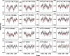 |
Fig. 7. Same as Fig. 5 but for the Hα line. In this case, the following larger bandwidths are used: 3.0 Å (first column), 5.0 Å (second column), 10.0 Å (third column), and 20.0 Å (fourth column). |
4.4. (Non-)detections of Hβ, Hγ, and Mg I?
Following Hα we analyzed the Hβ (λ4861.28 Å), Hγ (λ4340.46 Å) and Mg I (λ4571.10 Å) regions, with no clear signals observed in any case (see Fig. B.1).
We measure the absorption depth in the expected line position using a central bandwidth of 0.75 Å. For Hβ we use reference passbands of B = [4782.0, 4794.0] and R = [4926.0, 4938.0], measuring an absorption depth of 0.079 ± 0.059%. Using reference bandwidths of B = [4282.00, 4294.00] and R = [4366.0, 4378.0] for the Hγ line we get an absorption depth of 0.099 ± 0.077%. Finally, for Mg I, with B = [4492.00, 4504.00] and R = [4636.00, 4648.00], the measured absorption depth is 0.002 ± 0.034%.
For Hβ and Hγ the transmission spectrum is not totally flat but a lot of noise is concentrated in the expected line positions. Increasing the S/N by co-adding more transit observations is needed to determine the presence of these planetary absorption features.
5. Modeled Na I and Hα temperature profiles
Using high resolution spectroscopy we are not only able to detect chemical species in the atmosphere of exoplanets but also to resolve the spectral lines. When this happens, if the S/N of the final transmission spectrum is high enough, we can adjust isothermal models to different parts of these lines, whose origins reside in different layers of the atmosphere of the exoplanet and reconstruct the temperature profile.
To measure the temperature versus altitude profile from the Na I D transmission spectrum, we use the following atmospheric altitude, z(λ), equation given in Lecavelier Des Etangs et al. (2008):
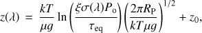 (1)
(1)where k is Boltzmann’s constant, T is the temperature, µ is the mean molecular weight of the atmospheric composition, g is the surface gravity, ξ = ξi/ξH is the elemental abundance of the chemical species i relative to the Hydrogen abundance, σ(λ) is the absorption cross section, Po is the pressure at the reference altitude, τeq is the optical depth at the transit radius, and RP is the radius of the planet. The z0 term is independent of the wavelength and can be determined by the altitude in the continuum wavelengths. This relation is derived from a plane-parallel atmosphere, assuming hydrostatic equilibrium and the ideal gas law.
The cross section, σ(λ), of each line is determined by mod-eling the lines as a Voigt profile,
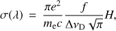 (2)
(2)where e is the electronic charge, me is the electron mass, c is the speed of light, f is the absorption oscillator strength, H is the Voigt profile, which includes thermal and natural broadening, and ∆νD is the Doppler width, given by
 (3)
(3)where νo the central frequency and µi the mean molecular weight of the chemical species are computed. We note that for the Na I doublet lines, σ(λ) is calculated for each line separately and the combined profile is calculated using σ(λ) = σ(λ)D2 + σ(λ)D1.
For MASCARA-2b, given the presence of Hα, we assume a mean molecular weight of µ = 1. We note that this assumption implies a totally dissociated hydrogen atmosphere, while in truth it could be only partially dissociated. In that latter case, the µ value would increase and the profile contrast would decrease for similar temperatures. On the other hand, we assume τeq = 0.56, as it is shown to be mainly constant for planets with RP/H ∼ 30−3000 by Lecavelier Des Etangs et al. (2008). We fix Po to 1 mbar. For the Na I, ξ is fixed to 1.995 × 10⁻⁶ as presented in Huitson et al. (2012) and, for Hα, we estimate ξ with the temperature-dependent relation presented in Huang et al. (2017),
 (4)
(4)where the peak Lyα intensity is J12 ≃ 0.1FLyC/∆νD, and FLyC ≃ 9.1 × 10⁴ erg cm−2 s−1 (Lund et al. 2017) is the flux received by the planet. As defined in Eq. 3, ∆νD depends on the local temperature. The values of the Na I and Hα parameters used are summarized in Table 4.
With this information and using the Levenberg–Marquardt algorithm through the leastsq tool (Jones et al. 2001), and similarly to Wyttenbach et al. (2015), we first determine the offset between the models and the data, z0, by fixing the temperature to Teq = 2260 K. Once the value is fixed, if the S/N were high enough, we could adjust models to different regions of the spectrum. However, the S/N of MASCARA-2b transmission spectrum is not sufficient to differentiate the wings regions (more ransit observations are needed). Still, it is possible to fit the lines core, observing that higher temperatures than Teq are required to explain the contrast measured in the Na I doublet and Hα lines. In order to fit the temperature of the lines core, we use the data within a 0.3 Å bandwidth in case of both Na I lines and 0.9 Å for Hα centered to the lines peak, which correspond to the measured FWHM of the lines. We note that each Na I D1 and D2 lines are adjusted separately, with best-fit models at T = 4240 ± 200 K and T = 4180 ± 310 K, respectively, which results in consistent temperatures taking into account the uncertainties. For the Hα line the best-fit model presents a temperature of 4330 ± 520 K. The best-fit models can be observed in Figs. 8 and 9.
As noted, the best-fit models shown here consider a mean molecular weight of µ = 1, which corresponds to a totally dissociated hydrogen atmosphere. For a molecular hydrogen atmosphere (µ = 2.3), the best-fit profiles in the lines core correspond to temperatures larger than 9000 K for the Na I (9250 ± 480 K) and Hα (9790 ± 1770 K) lines, i.e., larger than the effective temperature of the host star. However, atmospheres are expected to be heated up to 10 000–20 000 K, still producing absorption features in transmission. On the other hand, assuming an atomic hydrogen atmosphere (µ = 1.3) these temperatures decrease to 5400 ± 200 K and 5530 ± 770 K for the Na I and Hα lines core, respectively, and to ∼4000 K when a totally dissociated hydrogen atmosphere (µ = 1) is considered. The MASCARA-2b atmosphere could be only partially dissociated and, in that case, the µ value would be larger than 1. However, since the surface gravity of this planet has not been determined yet and only an upper limit has been estimated, we assume µ = 1 given that if the real g value were lower, it would lead to a similar effect in the temperature as decreasing µ, i.e., increasing the profiles contrast for similar temperatures. Thus, the 9250 ± 480 K and 9790 ± 1770 K for the Na I and Hα lines, respectively, obtained assuming µ = 1 and the g upper-limit value, can be considered as upper-limit estimations of the temperatures in these lines.
MASCARA-2b is part of the small sample of planets transiting an A-type star known to date, with effective temperatures higher than ∼7000 K. These planets typically receive a large amount of extreme ultraviolet radiation from its host star (∼9.1×10⁴ ergs s−1 cm−2 in case of MASCARA-2b), which produce the expansion of their atmosphere and excite the atomic hydrogen to produce Hα absorption and possibly abrasion of the atmosphere (Bourrier et al. 2016). Hα is commonly used as a stellar activity indicator because it is difficult to detect in ex-oplanet atmospheres, but not for planets orbiting A-type stars, which are not usually active. The measurement of a 0.63 ± 0.09% of Hα absorption in the atmosphere of MASCARA-2b corresponds to an effective radius, Rλ/RP, of 1.20 ± 0.04 and a temperature of 4330 ± 520 K. These values are obtained with only one transit observation, and considering the strong residuals observed in the Hβ and Hγ regions of MASCARA-2b transmission spectrum, by co-adding more transit observations we might be able to increase the S/N and study the temperature profile of the planet by observing these other Balmer lines and possibly calculate the lifetime of the atmosphere from escape rate measurements.
Summary of the Na I and Hα values assumed when fitting z(λ).
 |
Fig. 8. Fit of isothermal models to the transmission spectrum of MASCARA-2b in the Na I region. The vertical scale is atmospheric altitude in [km] assuming a planet-to-star radius ratio of |

 |
Fig. 9. Same as Fig. 8 but in the Hα region. The isothermal model at the equilibrium temperature (Teq = 2260 K), which is adjusted to the continuum, is shown in red. The blue line represents the model at 4330 ± 520 K, which is adjusted to the data contained in a 1.2 Å bandwidth centered to the peak position. Data and models are presented binned by 30 pixels. |
6. Conclusions
We observed one transit of MASCARA-2b, the hot Jupiter orbiting the fourth brightest star with a transiting planet, using the HARPS-North spectrograph. In that dataset, we resolve two spectral features centered on the atomic sodium (Na I) doublet position with an averaged absorption depth of 0.172 ± 0.029% for a 0.75 Å bandwidth, measuring line contrasts of 0.44 ± 0.11% (D2) and 0.37 ± 0.08% (D1), and FWHM of 0.26 ± 0.08 Å (D2) and 0.33 ± 0.08 Å (D1) from the Gaussian fit. The Na I TLC are also calculated, observing a large RM effect for small passbands, which is clearly diluted when the bandwidths are increased. After correcting for the RM and CLV effects using synthetic spectra, we measure a 0.200 ± 0.046% Na I transit absorption for a 0.75 Å passband that is consistent with the absorption depth values measured from the final transmission spectrum. We measure the temperature of the Na I lines core, resulting in T = 4240 ± 200 K and T = 4180 ± 310 K for the D2 and D1 lines, respectively, consistent within uncertainties. The S/N of the final transmission spectrum is not sufficient to adjust temperatures in different regions of the lines wings, however, we clearly observe that the equilibrium temperature (Teq = 2260 ± 50 K) cannot define the contrast observed in the Na I lines.
The same method is applied to Hα, observing a Gaussian feature centered at 6562.74 ± 0.08 Å with 0.63 ± 0.09% contrast and FWHM of 0.92 ± 0.16 Å. This absorption is also observed in the final TLC, presenting consistent absorption depths as those measured in the transmission spectrum of Hα. We measure a temperature of T = 4330 ± 520 K in the line core, corresponding to an effective radius Rλ/RP of 1.20 ± 0.04. Since MASCARA-2b is one of the most irradiated planets to date, we expect the atomic hydrogen to be excited and produce Hα absorption. This extreme UV radiation, as for other similar planets transiting A-type stars, can lead to the expansion and abrasion of their atmosphere.
We stress that the results presented in this work are obtained with only one transit observation as a consequence of the brightness of MASCARA-2 and the favorable physical parameters of MASCARA-2b for transmission spectroscopy. Thus more transits are desired to confirm these results. In particular, we observe residual absorption features in the Hβ and Hγ regions of MASCARA-2b transmission spectrum, but are not statistically significant. More transits would help to build up enough S/N to determine the presence of these planetary absorptions.
Currently, a small sample of planets are known that transits A-type stars. The study and comparison of these planets, which present different system properties and are irradiated different amounts of energy from their host stars, will help us to learn about their origin and evolution.
Acknowledgments
This work is based on observations made with the Ital-ian Telescopio Nazionale Galileo (TNG) operated on the island of La Palma by the Fundación Galileo Galilei of the INAF (Istituto Nazionale di Astrofisica) at the Spanish Observatorio del Roque de los Muchachos of the Instituto de Astrofisica de Canarias. This work is partly financed by the Spanish Ministry of Economics and Competitiveness through projects ESP2014-57495-C2-1-R and ESP2016-80435-C2-2-R. G.C. also acknowledges the support by the Natural Science Foundation of Jiangsu Province (Grant No. BK20151051) and the National Natural Science Foundation of China (Grant No. 11503088). I. Snellen acknowledges funding from the research programme VICI 639.043.107 funded by the Dutch Organisation for Scientific Research (NWO), and funding from the European Research Council (ERC) under the European Union’s Horizon 2020 research and innovation programme under grant agreement No 694513. J. I. G. H. and R. R. L. acknowledge the Spanish ministry project MINECO AYA2014-56359-P. J. I. González Hernández also acknowledges financial support from the Spanish Ministry of Economy and Competitiveness (MINECO) under the 2013 Ramón y Cajal programme MINECO RYC-2013-14875.
References
- Astudillo-Defru, N., & Rojo, P. 2013, A&A, 557, A56 [NASA ADS] [CrossRef] [EDP Sciences] [Google Scholar]
- Barnes, J. R., Haswell, C. A., Staab, D., & Anglada-Escudé, G. 2016, MNRAS, 462, 1012 [Google Scholar]
- Bourrier, V., Lecavelier des Etangs, A., Ehrenreich, D., Tanaka, Y. A., & Vidotto, A. A. 2016, A&A, 591, A121 [NASA ADS] [CrossRef] [EDP Sciences] [Google Scholar]
- Casasayas-Barris, N., Palle, E., Nowak, G., et al. 2017, A&A, 608, A135 [NASA ADS] [CrossRef] [EDP Sciences] [Google Scholar]
- Charbonneau, D., Brown, T. M., Noyes, R. W., & Gilliland, R. L. 2002, ApJ, 568, 377 [NASA ADS] [CrossRef] [Google Scholar]
- Chen, G., Guenther, E. W., Pallé, E., et al. 2017, A&A, 600, A138 [NASA ADS] [CrossRef] [EDP Sciences] [Google Scholar]
- Frasca, A., Freire Ferrero, R., Marilli, E., & Catalano, S. 2000, A&A, 364, 179 [NASA ADS] [Google Scholar]
- Heiter, U., Kupka, F., van’t Veer-Menneret, C., et al. 2002, A&A, 392, 619 [NASA ADS] [CrossRef] [EDP Sciences] [Google Scholar]
- Heng, K., Wyttenbach, A., Lavie, B., et al. 2015, ApJ, 803, L9 [Google Scholar]
- Huang, C., Arras, P., Christie, D., & Li, Z.-Y. 2017, ApJ, 851, 150 [NASA ADS] [CrossRef] [Google Scholar]
- Huitson, C. M., Sing, D. K., Vidal-Madjar, A., et al. 2012, MNRAS, 422, 2477 [NASA ADS] [CrossRef] [Google Scholar]
- Husser, T.-O., Wende-von Berg, S., Dreizler, S., et al. 2013, A&A, 553, A6 [NASA ADS] [CrossRef] [EDP Sciences] [Google Scholar]
- Jones, E., Oliphant, T., Peterson, P., et al. 2001, SciPy: Open source scientific tools for Python. http://www.scipy.org/ [Google Scholar]
- Lecavelier Des Etangs, A., Pont, F., Vidal-Madjar, A., & Sing, D. 2008, A&A, 481, L83 [NASA ADS] [CrossRef] [Google Scholar]
- Lodders, K. 2003, ApJ, 591, 1220 [NASA ADS] [CrossRef] [Google Scholar]
- Louden, T., & Wheatley, P. J. 2015, ApJ, 814, L24 [NASA ADS] [CrossRef] [Google Scholar]
- Lovis, C., Snellen, I., Mouillet, D., et al. 2017, A&A, 599, A16 [NASA ADS] [CrossRef] [EDP Sciences] [Google Scholar]
- Lund, M. B., Rodriguez, J. E., Zhou, G., et al. 2017, AJ, 154, 194 [NASA ADS] [CrossRef] [Google Scholar]
- Murgas, F., Pallé, E., Zapatero Osorio, M. R., et al. 2014, A&A, 563, A41 [NASA ADS] [CrossRef] [EDP Sciences] [Google Scholar]
- Nortmann, L., Pallé, E., Murgas, F., et al. 2016, A&A, 594, A65 [NASA ADS] [CrossRef] [EDP Sciences] [Google Scholar]
- Ohta, Y., Taruya, A., & Suto, Y. 2005, ApJ, 622, 1118 [NASA ADS] [CrossRef] [Google Scholar]
- Palle, E., Chen, G., Prieto-Arranz, J., et al. 2017, A&A, 602, L15 [NASA ADS] [CrossRef] [EDP Sciences] [Google Scholar]
- Parviainen, H. 2015, MNRAS, 450, 3233 [NASA ADS] [CrossRef] [Google Scholar]
- Parviainen, H., & Aigrain, S. 2015, MNRAS, 453, 3821 [Google Scholar]
- Redfield, S., & Linsky, J. L. 2008, ApJ, 673, 283 [NASA ADS] [CrossRef] [Google Scholar]
- Redfield, S., Endl, M., Cochran, W. D., & Koesterke, L. 2008, ApJ, 673, L87 [NASA ADS] [CrossRef] [MathSciNet] [Google Scholar]
- Sing, D. K., Huitson, C. M., Lopez-Morales, M., et al. 2012, MNRAS, 426, 1663 [NASA ADS] [CrossRef] [Google Scholar]
- Snellen, I. A. G., Albrecht, S., de Mooij, E. J. W., & Le Poole, R. S. 2008, A&A, 487, 357 [NASA ADS] [CrossRef] [EDP Sciences] [Google Scholar]
- Snellen, I. A. G., de Kok, R. J., le Poole, R., Brogi, M., & Birkby, J. 2013, ApJ, 764, 182 [NASA ADS] [CrossRef] [Google Scholar]
- Steck, D. A. 2010, Sodium D Line Data (Los Alamos National Observatory) [Google Scholar]
- Talens, G. J. J., Justesen, A. B., Albrecht, S., et al. 2018, A&A, 612, A57 [NASA ADS] [CrossRef] [EDP Sciences] [Google Scholar]
- Wiese, W. L., & Fuhr, J. R. 2009, J. Phys. Chem. Ref. Data, 38, 565 [NASA ADS] [CrossRef] [Google Scholar]
- Wilson, P. A., Sing, D. K., Nikolov, N., et al. 2015, MNRAS, 450, 192 [NASA ADS] [CrossRef] [Google Scholar]
- Wyttenbach, A., Ehrenreich, D., Lovis, C., Udry, S., & Pepe, F. 2015, A&A, 577, A62 [NASA ADS] [CrossRef] [EDP Sciences] [Google Scholar]
- Wyttenbach, A., Lovis, C., Ehrenreich, D., et al. 2017, A&A, 602, A36 [NASA ADS] [CrossRef] [EDP Sciences] [Google Scholar]
- Yan, F., Fosbury, R. A. E., Petr-Gotzens, M. G., et al. 2015, Int. J. Astrobiol., 14, 255 [CrossRef] [Google Scholar]
- Yan, F., Pallé, E., Fosbury, R. A. E., Petr-Gotzens, M. G., & Henning, T. 2017, A&A, 603, A73 [NASA ADS] [CrossRef] [EDP Sciences] [Google Scholar]
Appendix A
Two-dimensional representations
Two- dimensional representations of the observed spectra and the residuals after some reduction steps presented in Sect. 3 for the Na I (Fig. A.1) and Hα (Fig. A.2) regions. The vertical axis of each matrix represents the sequence number of the spectrum and the horizontal axis represents the wavelength. A detailed description can be seen in Fig. A.1 caption.
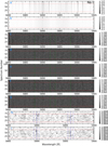 |
Fig. A.1. Two-dimensional representation of the MASCARA-2b spectra around Na I lines. The vertical axis of each panel represents the sequence number of the observed spectra (the time increases with the spectrum number); the red horizontal lines represent the limits between the in- and out-of-transit data. In the horizontal axis we present the wavelength in Å and the relative flux values are shown in the color bar. Panel a: original data after the normalization. Panel b: observed data after the telluric subtraction. Panels c, d, and e: residuals from the in-transit spectra and the master out spectrum ratio. The RM effect can be clearly observed in these panels. In panel d the data is binned by 20 pixels and in e we show the modeled RM residuals (without planetary absorption) obtained by applying to the modeled stellar spectra the same process as data from panels c and d. Panels f and g: residuals after correcting each single spectrum presented in c for the RM effect. We note in the process presented in Sect. 3 that the correction is applied to the final transmission spectrum after combining all In/Mout with the planet RV correction applied so as not to affect the planetary absorption. In panel g the data is binned by 20 pixels. The green vertical lines show the limits in wavelength of the RM effect (from −v sin i to +v sin i). Panel h: same as g decreasing the wavelength coverage and changing the contrast (see color-bar). Panels i: same as h after the planet RV correction. The blue vertical lines of panels h and i show the expected Na I position in wavelength due to the maximum and minimum RV of the planet during the transit (dashed line) and the mid-transit value, i.e., null RV (solid line). |
Appendix B
Hβ, Hγ and Mg I results
As referred in Sect. 4.4, other regions of the spectra are analyzed by applying the same method presented in Sect. 3. We present the resulting transmission spectra around Hβ, Hγ, and Mg I lines from which no clear conclusions can be extracted. The S/N needs to be increased by co-adding more transit observations to figure out the origin of their residuals.
 |
Fig. B.1. Transmission spectrum of MASCARA-2b atmosphere in the region of Hβ (top left), Hγ (top right), and Mg I (bottom). Transmission spectrum (light gray) and binned transmission spectrum by 30 pixels (black dots). The blue vertical line indicates the expected wavelength position in the planetary reference frame. |
All Tables
Summary of the measured relative absorption depth in [%] in the Na I D lines of the final transmission spectrum and the TLC of MASCARA-2b for various bandwidths.
Summary of the measured relative absorption depth in [%] in the Hα line of the final transmission spectrum and the TLC of MASCARA-2b for various bandwidths.
All Figures
|
Fig. 1. Normalized spectra of the telluric standard HR 7390 (blue) and MASCARA-2 (black) around the Na I region after their reduction with the HARPS DRS. In green we show the MASCARA-2 master out spectrum after the telluric correction. |
| In the text | |
|
Fig. 2. Modeled spectra of MASCARA-2 for various orbital phases of the planet using LTE and a spin-orbit angle of 0◦ (Talens et al. 2018) for the RM effect (top) and modeled RM and CLV effects in the final transmission spectrum (bottom). We note the large RM effect in the stellar lines. |
| In the text | |
|
Fig. 3. Transmission spectrum of MASCARA-2b atmosphere in the region of Na I D doublet. In the top panel the atmospheric transmission spectrum is presented in light gray. Black dots indicate the binned transmission spectrum by 10 pixels and the Gaussian fit to each Na I D lines is shown in red; its residuals are shown in the bottom panel. The expected wavelength position of the Na I doublet lines, in the planetary reference frame, are indicated with blue vertical lines. The uncertainties of the relative flux come from the error propagation of the photon and readout noise from the original data. |
| In the text | |
|
Fig. 4. Comparison between the transmission spectra obtained with (light blue line) and without (black line) stellar RV correction, before correcting for the final RM and CLV effects. In both cases the spectrum is binned by 10 pixels. The blue vertical lines show the expected wavelength position of the Na I D lines and the red horizontal line is the null-absorption reference. |
| In the text | |
|
Fig. 5. Na I TLC from HARPS-N observations of MASCARA-2b for four bandwidths: 0.75 Å (first column), 1.5 Å (second column), 3.0 Å (third column), and 5.0 Å (fourth column). In all panels, the light gray dots indicate the values from all the spectra, and the black dots the same data binned with 0.003 phase step. First row: observed TLC of the Na I D lines from our data reduction. The relative flux of the D1 and D2 lines is averaged. The red line indicates the modeled TLC, which is the combination of the best-fit Na I absorption and the CLV and RM effects (Yan et al. 2017). This model is calculated theoretically and there is no fitting to the data. Second row: the CLV + RM effects. The black line indicates the result of removing the Na I absorption model from the observed TLC. The modeled CLV and RM effects are shown in red. Third row: the Na I absorption light curve obtained dividing the observed TLC by the modeled CLV + RM effects (black line). The red line is the best-fit Na I absorption model. Fourth row: residuals between the observed TLC and the model. We note the different y-scale of the panels. |
| In the text | |
|
Fig. 6. Transmission spectrum of MASCARA-2b atmosphere in the region of Hα. Top panel: atmospheric transmission spectrum (light gray) and binned transmission spectrum by 30 pixels (black dots). The Gaussian fit is shown in red. Bottom panel: residuals of the Gaussian fit. The blue vertical line indicates the expected wavelength position in the planetary reference frame. |
| In the text | |
|
Fig. 7. Same as Fig. 5 but for the Hα line. In this case, the following larger bandwidths are used: 3.0 Å (first column), 5.0 Å (second column), 10.0 Å (third column), and 20.0 Å (fourth column). |
| In the text | |
|
Fig. 8. Fit of isothermal models to the transmission spectrum of MASCARA-2b in the Na I region. The vertical scale is atmospheric altitude in [km] assuming a planet-to-star radius ratio of |
| In the text | |
|
Fig. 9. Same as Fig. 8 but in the Hα region. The isothermal model at the equilibrium temperature (Teq = 2260 K), which is adjusted to the continuum, is shown in red. The blue line represents the model at 4330 ± 520 K, which is adjusted to the data contained in a 1.2 Å bandwidth centered to the peak position. Data and models are presented binned by 30 pixels. |
| In the text | |
|
Fig. A.1. Two-dimensional representation of the MASCARA-2b spectra around Na I lines. The vertical axis of each panel represents the sequence number of the observed spectra (the time increases with the spectrum number); the red horizontal lines represent the limits between the in- and out-of-transit data. In the horizontal axis we present the wavelength in Å and the relative flux values are shown in the color bar. Panel a: original data after the normalization. Panel b: observed data after the telluric subtraction. Panels c, d, and e: residuals from the in-transit spectra and the master out spectrum ratio. The RM effect can be clearly observed in these panels. In panel d the data is binned by 20 pixels and in e we show the modeled RM residuals (without planetary absorption) obtained by applying to the modeled stellar spectra the same process as data from panels c and d. Panels f and g: residuals after correcting each single spectrum presented in c for the RM effect. We note in the process presented in Sect. 3 that the correction is applied to the final transmission spectrum after combining all In/Mout with the planet RV correction applied so as not to affect the planetary absorption. In panel g the data is binned by 20 pixels. The green vertical lines show the limits in wavelength of the RM effect (from −v sin i to +v sin i). Panel h: same as g decreasing the wavelength coverage and changing the contrast (see color-bar). Panels i: same as h after the planet RV correction. The blue vertical lines of panels h and i show the expected Na I position in wavelength due to the maximum and minimum RV of the planet during the transit (dashed line) and the mid-transit value, i.e., null RV (solid line). |
| In the text | |
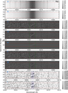 |
Fig. A.2. Same as Fig. A.1 but for the Hα line. |
| In the text | |
|
Fig. B.1. Transmission spectrum of MASCARA-2b atmosphere in the region of Hβ (top left), Hγ (top right), and Mg I (bottom). Transmission spectrum (light gray) and binned transmission spectrum by 30 pixels (black dots). The blue vertical line indicates the expected wavelength position in the planetary reference frame. |
| In the text | |
Current usage metrics show cumulative count of Article Views (full-text article views including HTML views, PDF and ePub downloads, according to the available data) and Abstracts Views on Vision4Press platform.
Data correspond to usage on the plateform after 2015. The current usage metrics is available 48-96 hours after online publication and is updated daily on week days.
Initial download of the metrics may take a while.