| Issue |
A&A
Volume 616, August 2018
|
|
|---|---|---|
| Article Number | A178 | |
| Number of page(s) | 10 | |
| Section | Planets and planetary systems | |
| DOI | https://doi.org/10.1051/0004-6361/201832721 | |
| Published online | 03 September 2018 | |
Opposition effect on S-type asteroid (25143) Itokawa
1
Department of Physics and Astronomy, Seoul National University,
1 Gwanak,
Seoul
08826, Republic of Korea
e-mail: This email address is being protected from spambots. You need JavaScript enabled to view it.
; This email address is being protected from spambots. You need JavaScript enabled to view it.
2
University of Science & Technology,
Daejeon
34113, Republic of Korea
3
Korea Astronomy and Space Science Institute,
Daejeon
34055, Republic of Korea
Received:
21
January
2018
Accepted:
11
May
2018
Abstract
Aims. The opposition effect has been detected on solar system bodies such as asteroids and comets. Two mechanisms have been proposed to explain the effect: the shadow-hiding opposition effect (SHOE) and the coherent backscattering opposition effect (CBOE). The Hayabusa asteroid sample return mission provides a unique opportunity to investigate the opposition effect on disk-resolved images of the S-type asteroid (25413) Itokawa at very small phase angles α.
Methods. We made use of the data taken at α = 0.°04–2.°54 using the Asteroid Multi-band Imaging Camera (AMICA) on UT 2005 October 13. Comparing sets of two images taken at different phase angles, we derived the opposition slope parameter (SOE) that characterizes a linear increase in the reflectance I∕F per unit phase angle.
Results. We found that (i) SOE is less dependent on the incidence and emission angles; (ii) the reflectance increases nonlinearly toward the opposition at small angles with α ≲ 1.°4, showing a good correlation between mean I∕F and SOE; and (iii) SOE becomes nearly constant at α ≳ 1.°4 and shows no clear correlation between I∕F and SOE.
Conclusions. From these results, we conjecture that CBOE is dominant at α ≲ 1.°4, while SHOE is dominant at α ≳ 1.°4.
Key words: minor planets, asteroids: general / minor planets, asteroids: individual: Itokawa
© ESO 2018
1 Introduction
It is widely known that the brightness of reflected light from solar system bodies increases nonlinearly near zero phase angle (i.e., a Sun–object–observer angle of α ~ 0°). This phenomenon is known as the “opposition effect” and has been observed on a wide variety of objects, such as Mars (O’Leary & Jackel 1970; Thorpe 1978), outer satellites (Hapke 1990), Kuiper Belt Objects (KBOs; Belskaya et al. 2003), the Moon (Lyot 1929; Buratti et al. 1996), and the Saturnian ring (Franklin & Cook 1964; French et al. 2007). For asteroids, Gehrels (1956) detected the opposition effect on (20) Massalia for the first time. Later, the effect was confirmed on different types of asteroids, such as E-type (Harris et al. 1989), V-type (Hasegawa et al. 2014), C-type (Harris & Young 1988), and S-type asteroids (Gehrels 1956; Gehrels & Taylor 1977; Dovgopol et al. 1992). Thus, the opposition effect is essentially detected for all types of atmosphere-less bodies in the solar system.
Two mechanisms have been suggested to explain the opposition effect: the shadow-hiding opposition effect (SHOE) and the coherent backscattering opposition effect (CBOE). SHOE is attributed to the fact that shadowed areas, which are crated by surface grains and the walls of particulate tunnels inside the surface medium as well as by the surface roughness, decrease when viewed from the direction of the light source (i.e., α ~ 0°). The surface brightness consequently increases with respect to the surrounding area near the opposition region (Hapke 2012b). It is suggested that the structural characteristics of the particulate medium, such as compressibility and particle size distribution, could be significant factors in determining the profile of SHOE (Hapke 1986, 2012b; Stankevich et al. 1999). In contrast, CBOE occurs when incident wavefronts of light constructively interfere in opposite directions along the particulate medium in the same path as the light. At opposition, these rays interfere with each other through multiple scattering inside a single particle or among discrete particles. Several studies (e.g., Shkuratov 1989; Muinonen & Lumme 1991; Mishchenko & Dlugach 1993; Hapke et al. 1993; Nelson et al. 1998; Muinonen et al. 2002, 2012) have been performed to study the opposition effect using various approaches, including theoretical and experimental approaches as well as phenomenological approaches via observations. It has been suggested that it might be possible to distinguish CBOE and SHOE using polarimetric data (e.g., Hapke et al. 1993).
Although the opposition effect has been observed on a variety of objects, as described above, it is still challenging to pinpoint the cause of the effect using photometric data because CBOE and SHOE can result in similar profiles in the photometric data (usually phase curves of the reflectances; Hapke 1986), although SHOE shows a phase curve that is broader than that of CBOE (Hapke et al. 1993). For example, Hapke et al. (1993) insisted on the dominance of CBOE, while Buratti et al. (1996) argued for SHOE on the lunar surface. Helfenstein et al. (1997) suggested that the lunar opposition effect could be explained by a combination of CBOE and SHOE. In case of the lunar surface, it seems that the CBOE is dominant atvery small phase angles, but SHOE is stronger in a broad range of small phase angles (Muinonen et al. 2002). However, there appears to be no consensus concerning the mechanism of the opposition effect on asteroidal surfaces.
Here, we provide new research on an S-type asteroid, (25143) Itokawa (hereafter, Itokawa), which is a target asteroid of the Hayabusa mission. During the rendezvous phase, the spacecraft was operated approximately on the line between Sun and the asteroid. The geometry is favorable for investigating the opposition effect. In 2005 October, we intentionally acquired data at very small phase angles using the onboard telescopic camera (AMICA) courtesy of the project team by inserting the spacecraft into the line between the Sun and Itokawa. The dataset provides a unique opportunity to investigate the opposition effect on an S-type asteroid. In this paper, we analyze the multiband images taken by AMICA through four bandpass filters and examine the reflectance slopes near opposition. We describe ourAMICA image analysis method in Sect. 2, present the results in Sect. 3, and discuss our findings in Sect. 4. Finally, we summarize our study in Sect. 5.
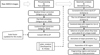 |
Fig. 1 Flow chart of the data analysis process for this study using Hayabusa/AMICA data. |
2 Image analysis
2.1 AMICA observation near opposition
The data presented in this study were all obtained with AMICA. This instrument covers the visible to near-infrared wavelengths (381–1008 nm). AMICA was designed for the scientific investigation of Itokawa during the rendezvous phase (Ishiguro et al. 2010). The specification and performance are described in Ishiguro et al. (2010) and Ishiguro (2014). We followed the data reduction method described in these papers, but slightly modified the process for the opposition effect analysis presented below. Figure 1 presents the data reduction flow diagram.
On 2005 October 13, the spacecraft was intentionally located on the line between the Sun and the asteroid to investigate the opposition effect when it was at 8.23–8.64 km from the surface. Although we were not able to detect the exact opposition point from the distance because of an imperfect control of the trajectory, we obtained valuable opposition data at phase angles of α = 0.°05–2.°54 using four different filters, b (429 nm), v (553 nm), w (700 nm), and p (960 nm), to study the wavelength dependence of the opposition effect. We employed a 4 × 4 binning mode for downlink to reduce the total amount of data. For the scientific analysis, we downloaded the data in lossless compressionmode. Table 1 shows the summary of the data and their phase angle coverages. It is important to note that the phase angle differs in the field of view because the apparent size of the asteroid exceeded ≳1.°5 (unlike in ground-based telescopic observations). In addition, the phase angle changed between exposures due to the movement of the spacecraft with respect to the Sun–asteroid vector. Two sets of observations were conducted on the eastern and western sides of Itokawa. On the western side, two subsets of observations were conducted at a time interval of ~12 h (i.e., one rotational period) to capture the reflectance changes due to the movement of the spacecraft (i.e., the change in phase angle). However, on the eastern side, which includes the sampling site (i.e., the Muses Sea), a subset of observational data was not obtained at small phase angles because of unfavorable observation timing. Therefore, we made pairs of AMICA images on the western side that observed twice at two different phase angles with four different filters. In this paper, we refer to these two sets on the western side to as Sets 1 and 2.
Figure 2 shows the example images of each set taken with the v-band filter. At first glance, the observed images show a uniform surface brightness. The geological features (e.g., boulders and craters) are mostly eliminated, and an even brightness distribution is shown. For example, the largest boulder, Yoshinodai, is entirely obscured and blends in with the surrounding area (Fig. 2, bottom panel). However, there is still regional variation in the reflectance, which would be due to the inherent optical properties of the materials in these regions rather than the geological features, as we show below.
2.2 Data processing
Our data processing method consists of the following three major steps (see also Fig. 1):
- 1.
Pre-processing and flux calibration. We followed the processing methods presented in Ishiguro et al. (2010) and Ishiguro (2014). However, we updated the calibration factors, as described in Table 2. The details are available in Sect. 2.2.1.
- 2.
Geometry analysis. Light illumination angles, that is, incidence, emission, and phase angles (i, e, and α), are calculated using the simulation tool “plate_renderer” together with kernels provided by the project team. The details are available in Sect. 2.2.2
- 3.
Derivation of a parameter that characterizes the strength of the opposition effect (SOE). Three criteria were applied to clean up the SOE data. See the details in Sects. 2.2.4 and 2.2.5.
Summary of AMICA images.
2.2.1 Pre-processing
The raw AMICA images went through a few steps to convert the raw images into reduced images. We first subtracted a read-out smear, which is the vertical structure during photon transfer. Second, we subtracted a constant bias value from the raw images and divided them by flat images in each band. Additionally, we subtracted the scattered light components using the point spread functions (PSFs) of each AMICA filter (see the details in Ishiguro 2014).
To fit the reflectance of AMICA images to ground observation data (Binzel et al. 2001; Lowry et al. 2005), the scale factorsgiven in Ishiguro et al. (2010) were used. These factors are determined without consideration of the scattered light inside AMICA optics, however, because the subtraction technique (see Ishiguro 2014) was established after the publication of Ishiguro et al. (2010). We updated the scale factors for each of the four bands (b, v, w, and p) after subtracting the scattered light, following the technique in the above paper. Table 2 presents the updated scaling factors.
We converted reduced AMICA intensities into I∕F values that represent absolute reflectances, known as radiance factors, which are the ratio between the reflected intensity from the surface and solar irradiance at a given distance and wavelength assuming a Lambertian surface. The mean I∕F values of Itokawa’s disk in each set are approximately 0.19–0.2 (b), 0.23–0.24 (v), 0.26–0.27 (w), and 0.23–0.25 (p-band).
2.2.2 Geometry of Itokawa
Geometric information (i.e., i, e, and α) is required to examine the opposition effect. Because Itokawa has an irregular shape, it is inadequate to approximate a simplified shape such as an ellipsoid. We employed the shape model of Itokawa taken from the Hayabusa mission (Gaskell et al. 2006).
We used plate_renderer, which was developed by Naru Hirata (University of Aizu, Japan), for the calculations of this geometric information. This tool provides a view of AMICA at a given time based on the shape model of Itokawa andthe NASA SPICE toolkit, which requires the position of the spacecraft and planetary objects as kernels. This tool produces the simulated AMICA image and extra images that contain geometrical information at a given time in the FITS format. This tool is similar to OASIS, which is a simulation tool for the Rosetta mission (Jorda et al. 2010; Spjuth et al. 2012). We obtained the plate ID of the shape model as well as the geometric information.
Figure 3 shows the maps of I∕F in the v-band (left panel) and their corresponding phase angles α (right panel). As described above, the phase angle of all images taken at opposition reaches below ~2.°5. We realized that the average phase angle of Set 1 is smaller than that of Set 2 (because Set 1 data were taken when the spacecraft was almost on the Sun–asteroid line). Centering on the bottom part of these maps at the opposition point, the phase angle is distributed in an arc shape (see the right columns of Fig. 3).
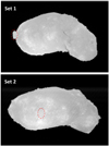 |
Fig. 2 Example images near opposition taken on 2005 October 13. The red dashed ellipse in the bottom panel indicates the location of Yoshinodai, the largest boulder on Itokawa. |
Scale factors for AMICA image calibration with respect to the v-band.
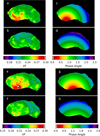 |
Fig. 3 Panels a and b: I∕F maps of Set 1. Panels c and d: phase angle maps for the corresponding I∕F maps. The opposition is located at the bottom of these maps. The reddish parts in the top left map correspond to a high-albedo region that is close to the opposition. Panels e and f: I∕F maps of Set 2. Panels g and h: phase angle maps for the corresponding I∕F maps. The opposition is located at the bottom of these maps. |
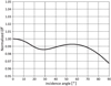 |
Fig. 4 Relationship between the incidence angle and I∕F, which is computed based on the Hapke model with the parameters given in Lederer et al. (2008). The horizontal axis can be regarded as the emission angle due to the small phase angle (assuming zero azimuth angle). |
2.2.3 Dependency of incident and emission angles on I∕F
To examine the incident angle dependence of I∕F values near opposition, we tentatively calculated this relation using a theoretical model, the so-called Hapke model (Hapke 1981, 1984, 1986, 2002, 2012a). This model is commonly used to derive properties on airless surfaces. We employed the 1984 version of the Hapke model. We applied the Hapke parameters of Itokawa in the Johnson Cousins V -band, which were determined from ground-based observations (Lederer et al. 2008). Note that the AMICA v-band filter is compatible with the V -band filter (Ishiguro et al. 2010) such that this model simulation provides a benchmark for evaluating AMICA/Itokawa data. Figure 4 shows the results of the calculation. We found that there is no significant (<2%) change in I∕F values at the incident angle ≲60–70°, ensuring the observed flat intensity distribution, as described above. It is possible to regard the incidence and emission angles as nearly the same at the smallest phase angles in the case of a zero azimuth angle. Therefore, Fig. 4 shows not only the relationship between the incidence angle and normalized I∕F, but also that between emission angle and normalized I∕F. This fact was used as a criterion that is described in Sect. 2.2.5. In general, one should consider the light illuminationconditions (i.e., incident and phase angles) to derive the I/F. However, as described below, we realized that the corrections for the illumination angles are not required for the data at small phase angles.
2.2.4 Characterization of the opposition effect
Although we acknowledge that the Hapke model is widely used in planetary science, it is difficult to obtain a unique solution for each parameter because the parameters compensate for one another to create almost identical phase angle profiles of I∕F. To avoid the complexity of the model, we considered a simple model here. We thus defined a parameter to characterize the slope of the opposition effect (hereafter, SOE) at small phase angles. This parameter originates from the slope of a linear function. We compared I∕F values of a set of images at the same position on the asteroid and calculated SOE, defined in the following equation:
 (1)
(1)
where subscripts 1 and 2 mean the indexes of an image in each set, where image 1 was taken at a larger phase angle than that for image 2. The second subscript, i, denotes a coordinate (i.e., corresponding pixel) in an image.  and Δα are differences in I∕F and α between images 2 and 1.
Because the rotational phases of the images in the set do not perfectly match one another, we needed further processing to extract data points. We reference the plate ID of Itokawa’s shape model by means of the plate_renderer. We used the highest-resolution shape model (a total of 3 145 728 facets), which has a better resolution than the opposition images taken with the 4 × 4 binning mode.
2.2.5 Criteria for the slope parameter
In the last stage of the data analysis, we considered several criteria to extract clean slope parameters. First, we applied the criterion Δ α > 0.°3 because the error of SOE can be magnified when Δα is small (Criterion 1). In fact, there are noisy data (see Fig. 5, to the right of the dashed line) where SOE fluctuated significantly. Second, as we described above, some portions of the data have low quality because of the rotation. This effect is severe at the edge of the asteroid in the equatorial region. We ignored data around the edge (approximately five pixels from the rim, Criterion 2). Finally, we derived the slope parameter (SOE) of Itokawa taking into account two cases: (1) without i and e limitations, and (2) with i ~ e <60 ° (Criterion 3). Criterion 3 is based on the fact that I∕F is less dependent on the incident and emission angles (see Sect. 2.2.3). We do not employ Criterion 3 in the following discussion because it does not exert any critical influence on the result.
3 Results
Figure 5 illustrates the maps of the slope parameter, SOE, without applying any of the criteria presented in Sect. 2.2.5. Because the reflectance decreases as the phase angle increases, SOE should have negative values in our definition. In the sub-panels of Fig. 5, a steeper SOE appears as α decreases (see the darkest portion in each column). Comparing data from different bands, we found that the w- and p-band data indicate steeper slopes than the b- and v-band data with a value of SOE < −0.05. Furthermore, we realized that the area of the steeper slope in Set 1 is larger than that in Set 2. This result is understandable because the Set 1 images were taken at a smaller phase angle. As we described above, the largest boulder, Yoshinodai, is indistinguishable in Fig. 5, indicating that SOE is less dependent on geological slope.
Figure 6 represents SOE with respect to the average phase angle in two images. We made Fig. 6 using Set 1 images and Fig. A.1 using Set 2 images (see Appendix A). Each panel in these figures illustrates SOE for four different wavelengths (b, v, w, and p bands) in a counterclockwise direction from top left. We calculated the median value and the standard deviation with a bin size of 0.°05 to derive the mean phase angle and the errors (Fig. 6). As we described above, there is no noticeable difference in α–SOE plots between Criterion 3 (1) and (2). Accordingly, we do not impose any limitation on the incident and emission angles in these plots. This fact is in accordance with the disappearance of Yoshinodai in Fig. 5.
A remarkable fact in Fig. 6 is that the median values at small phase angle have slopes steeper than those at large phase angles, suggesting that I∕F increases nonlinearly as α decreases. The inflection points may exist in 1.°2 < α <1.°4 from a visual inspection. We also found that the trend is weak in the p-band. The red and blue lines in Fig. 6 are fitted lines to determine the inflection points. From the fitting with a linear function, the inflection point (i.e., the intersection of red and blue lines) of SOE was determined to be 1.°3 ± 0.°02.
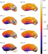 |
Fig. 5 Maps of the slope parameter (SOE) for Set 1 (left panel) and Set 2 (right panel) at different wavelengths. The dark blue parts correspond to regions with steeper slope (i.e., smaller SOE), while the redparts represent a shallower slope (i.e., higher SOE). The opposition point is indicated by red arrows in the bottom panels. Green dashed lines separate regions where Δ α is >0.°3 (leftward) and <0.°3 (rightward), respectively, suggesting that the data to left side of the line satisfied Criterion 1 (see Sect. 2.2.5). |
4 Discussion
As shown in Fig. 6, the SOE profiles show steep slopes at small phase (α < 1.°3) angles and moderate slopes at large phase angles (α > 1.°3). What does this result suggest?
Itokawa is classified as an S-type asteroid. Taking advantage of our data at small phase angles, we calculated the average I∕F at α < 2.°23 following the method in Spjuth et al. (2012) and found the value to be  = 0.23. The value at opposition is known as the normal albedo, which is analogous to the geometric albedo. The geometric albedo of Itokawa is typical of S-type asteroids (0.258 ± 0.087, DeMeo & Carry 2013; and 0.208 ± 0.079, Usui et al. 2013). It is known that CBOE and SHOE can occur simultaneously on asteroids with such moderate albedo (Belskaya & Shevchenko 2000; Shkuratov & Helfenstein 2001). Accordingly, our data may suggest that these two mechanisms produce different results in the SOE profiles.
We further examined SOE at small and large phase angles (which are referred to as Domain I and Domain II) separately to determine the I∕F-dependence. We chose the boundary phase angle at α =1.°4 (slightly larger than the value we derived above, but we confirmed that the difference is insignificant). Figure 7 shows the relation between mean I∕F (horizontal axis) and SOE (vertical axis). To reduce the measurement errors of I∕F and SOE, we calculated the average values in small circular areas on the surface. We thus chose 36 small circular areas (~ 24 m 2) on the asteroid surface from Domains I and II, respectively, and calculated the average SOE values and their the standard deviations (the error bars in Fig. 7) for each area. In addition, we derived the average I∕F values in each circular area using Sets 1 and 2, and placed them along the abscissa.
Based on the figure, we found a correlation between I∕F and SOE in Domain I (i.e., α < 1.°4) but little correlation between them in Domain II (i.e., α > 1.°4). We calculated Pearson’s correlation coefficients ρ of these two parameters in each band; they are summarized in Table 3. It is clear that SOE and I∕F has a strong negative correlation when α < 1.°4 (ρ ≲−0.7, except for p-band data in Set 1) but an insignificant correlation when α > 1.°4 (|ρ|≈ 0). Although we do not know why the p-band data in Set 1 do not show a trend consistent with that of other bands in Domain I, we can conclude that I∕F exerts a major influence on SOE at the smallest phase angles.
The strength of the opposition effect via CBOE may be correlated with reflectance because multiple scattering, which favorably occurs among particles with high reflectance, is responsible for CBOE (Hapke et al. 1998). S-type asteroids have the highest spectra of all images in the w filter (Binzel et al. 2001), therefore CBOE appears to be strongest here. However, SHOE results from macroscopic roughness, which is less independent of wavelength and reflectance. Therefore, we conclude that our opposition effect on Itokawa is mostly caused by CBOE at α ≲ 1.°4 and by SHOE at α ≳ 1.°4. It is interesting to note that this opposition surge associated with CBOE is difficult to observe on the Moon during lunar eclipses and on Itokawa with a wide-angle camera (i.e., ONC-W) because the surge would be within the shadows of the Earth and observers. We posit that the ability to employ telescopic imaging at different wavelengths as well as over large variations in I∕F would enable distinguishing these effects.
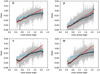 |
Fig. 6 Opposition slope for Set 1 with respect to the mean phase angle. We adopted Criterion 3 (e.g., no i and e limitation). The wavelengths of the bands become longer counterclockwise from the top left. Gray dots present SOE for each pixel, and open circles with vertical error bars show the median values and the standard deviations of each pixel in the 0.°05 bin of the phase angle. We fit the median values at smaller and larger phase angles with lines (see the Sect. 3). |
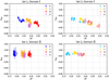 |
Fig. 7 Slope parameter (SOE) based on manual extraction from image. The first column (top left and bottom left panels) is the relation between I∕F and SOE for Domain I, and the second column (top right and bottom right panels) is that for Domain II. I∕F is the representative value for an average of two images in each band and each set. Square symbols correspond to data from Set 1, while circles represent Set 2 data. Different colors coincide with the different bands of AMICA. |
Pearson’s correlation coefficient between slope parameter (SOE) and I∕F in each band: b, v, w, and p.
5 Summary
We examined the opposition effect on S-type asteroid Itokawa using images taken with AMICA. We undertook a disk-resolving analysis and derived an opposition slope parameter (SOE), which characterizes how strong the opposition effect is. Our findings are listed below:
-
SOE is independent of the observed geometry (i.e., the angle of incidence and emission). The result is supported by the Hapke’s bidirectional reflectance model with parameters obtained by ground-based observations.
-
The bidirectional reflectance increases nonlinearly toward the opposition point at α ≲ 1.°4, showing a good correlation between mean I∕F and SOE. In contrast, mean SOE becomes nearly constant at α ≳ 1.°4, showing no clear correlation between mean I∕F and SOE.
-
These results suggest that CBOE is dominant in the near-opposition domain with a clear correlation, while SHOE plays the primary role at α ≳ 1.°4.
-
The geometric albedo was derived to be 0.23 ± 0.02 as a by-product of this work.
Acknowledgements
This work was conducted at Seoul National University as a part of master thesis of ML (currently at KASI and UST) under the supervision of MI. It was supported by the National Research Foundation of Korea (NRF), which is funded by the South Korean government (MEST) (Grant No. 2015R1D1A1A01060025). We wish to thank N. Hirata at the University of Aizu for providing plate_renderer and Y. Kim and Y.P. Bach at Seoul National University, who gave valuable comments. We are also grateful to H.-K. Moon, M.-J. Kim, M. Jeong, and Y.-J. Choi at the Korea Astronomy and Space Science Institute (KASI) for their useful comments and their encouragement. Finally, we cordially thank the Hayabusa operation team members for providing the precious opportunity to acquire the data despite the tight schedule during the mission period.
Appendix A Additional figure for Sect. sectionlinking 3
Figure A.1 shows the relation of the opposition slope with respect to the mean phase angle. We used data of Set 2 with the same method as described in Sect. 2.2.4.
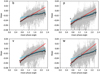 |
Fig. A.1 Slope of the opposition effect (SOE) for Set 2 with respect to the mean phase angle. This figure applied Criterion 3 (1) (e.g., no i and e limitation). The details of the plots are described in Sect. 3. |
References
- Belskaya, I. N., & Shevchenko, V. G. 2000, Icarus, 147, 94 [NASA ADS] [CrossRef] [Google Scholar]
- Belskaya, I. N., Barucci, A. M., & Shkuratov, Y. G. 2003, Earth, Moon and Planets, 92, 201 [Google Scholar]
- Binzel, R. P., Rivkin, A. S., Bus, S. J., Sunshine, J. M., & Burbine, T. H. 2001, Meteoritics and Planetary Science, 36, 1167 [NASA ADS] [CrossRef] [Google Scholar]
- Buratti, B. J., Hillier, J. K., & Wang, M. 1996, Icarus, 124, 490 [NASA ADS] [CrossRef] [Google Scholar]
- DeMeo, F. E., & Carry, B. 2013, Icarus, 226, 723 [NASA ADS] [CrossRef] [Google Scholar]
- Dovgopol, A. N., Kruglyi, I. N., & Shevchenko, V. G. 1992, Acta Astron., 42, 67 [NASA ADS] [Google Scholar]
- Franklin, F. A., & Cook, A. F. 1964, AJ, 70, 704 [NASA ADS] [CrossRef] [Google Scholar]
- French, R. G., Verbiscer, A., Salo, H., McGhee, C., & Dones, L. 2007, PASP, 119, 623 [NASA ADS] [CrossRef] [Google Scholar]
- Gaskell, R., Barnouin-Jha, O., Scheeres, D., et al. 2006, AIAA/AAS Astrodynamics Specialist Conference and Exhibit (Reston, VA: American Institute of Aeronautics and Astronautics) [Google Scholar]
- Gehrels, T. 1956, ApJ, 123, 331 [NASA ADS] [CrossRef] [Google Scholar]
- Gehrels, T., & Taylor, R. C. 1977, AJ, 82, 229 [NASA ADS] [CrossRef] [Google Scholar]
- Hapke, B. 1981, J. Geophys. Res., 86, 3039 [Google Scholar]
- Hapke, B. 1984, Icarus, 59, 41 [NASA ADS] [CrossRef] [Google Scholar]
- Hapke, B. 1986, Icarus, 67, 264 [NASA ADS] [CrossRef] [Google Scholar]
- Hapke, B. 1990, Icarus, 88, 407 [NASA ADS] [CrossRef] [Google Scholar]
- Hapke, B. 2002, Icarus, 157, 523 [NASA ADS] [CrossRef] [Google Scholar]
- Hapke, B. 2012a, Icarus, 221, 1079 [NASA ADS] [CrossRef] [Google Scholar]
- Hapke, B. 2012b, Theory of Reflectance and Emittance Spectroscopy (Cambridge: Cambridge University Press) [Google Scholar]
- Hapke, B. W., Nelson, R. M., & Smythe, W. D. 1993, Science, 260, 509 [NASA ADS] [CrossRef] [PubMed] [Google Scholar]
- Hapke, B., Nelson, R., & Smythe, W. 1998, Icarus, 133, 89 [NASA ADS] [CrossRef] [Google Scholar]
- Harris, A., & Young, J. 1988, Abstracts of the Lunar and Planetary Science Conference, 19, 447 [NASA ADS] [Google Scholar]
- Harris, A. W., Young, J. W., Contreiras, L., et al. 1989, Icarus, 81, 365 [NASA ADS] [CrossRef] [Google Scholar]
- Hasegawa, S., Miyasaka, S., Tokimasa, N., et al. 2014, PASJ, 66, 89 [NASA ADS] [Google Scholar]
- Helfenstein, P., Veverka, J., & Hillier, J. 1997, Icarus, 128, 2 [NASA ADS] [CrossRef] [Google Scholar]
- Ishiguro, M. 2014, PASJ, 66, 55 [NASA ADS] [CrossRef] [Google Scholar]
- Ishiguro, M., Nakamura, R., Tholen, D. J., et al. 2010, Icarus, 207, 714 [NASA ADS] [CrossRef] [Google Scholar]
- Jorda, L., Spjuth, S., Keller, H. U., Lamy, P., & Llebaria, A. 2010, in Proc. SPIE, eds. C. A. Bouman, I. Pollak, & P. J. Wolfe, 7533, 753311 [CrossRef] [Google Scholar]
- Lederer, S. M., Domingue, D. L., Thomas-Osip, J. E., et al. 2008, Earth, Planets, and Space, 60, 49 [NASA ADS] [CrossRef] [Google Scholar]
- Lowry, S. C., Weissman, P. R., Hicks, M. D., Whiteley, R. J., & Larson, S. 2005, Icarus, 176, 408 [NASA ADS] [CrossRef] [Google Scholar]
- Lyot, B. 1929, Ann. Obs. Paris, 8, 169 [Google Scholar]
- Mishchenko, M. I., & Dlugach, J. M. 1993, Planet. Space Sci., 41, 173 [NASA ADS] [CrossRef] [Google Scholar]
- Muinonen, K.,& Lumme, K. 1991, in Origin and Evolution of Interplanetary Dust: Proceedings of the 126th Colloquium of the International Astronomical Union, eds. A. C. Levasseur-Regoud & H. Hasegawa, Astrophysics and Space Science Library, 173, 159 [NASA ADS] [CrossRef] [Google Scholar]
- Muinonen, K., Piironen, J., Shkuratov, Y. G., Ovcharenko, A., & Clark, B. E. 2002, Asteroid Photometric and Polarimetric Phase Effects (Arizona: The University of Arizona Press), 123 [Google Scholar]
- Muinonen, K., Mishchenko, M. I., Dlugach, J. M., et al. 2012, ApJ, 760, 118 [NASA ADS] [CrossRef] [Google Scholar]
- Nelson, R. M., Hapke, B. W., Smythe, W. D., & Horn, L. J. 1998, Icarus, 131, 223 [NASA ADS] [CrossRef] [Google Scholar]
- O’Leary, B., & Jackel, L. 1970, Icarus, 13, 437 [NASA ADS] [CrossRef] [Google Scholar]
- Shkuratov, Y. G. 1989, Sol. Syst. Res., 23, 111 [Google Scholar]
- Shkuratov, Y. G., & Helfenstein, P. 2001, Icarus, 152, 96 [NASA ADS] [CrossRef] [Google Scholar]
- Spjuth, S., Jorda, L., Lamy, P. L., Keller, H. U., & Li, J.-Y. 2012, Icarus, 221, 1101 [NASA ADS] [CrossRef] [Google Scholar]
- Stankevich, D. G., Shkuratov, Y. G., & Muinonen, K. 1999, J. Quant. Spec. Rad. Transf., 63, 445 [Google Scholar]
- Thorpe, T. E. 1978, Icarus, 36, 204 [NASA ADS] [CrossRef] [Google Scholar]
- Usui, F., Kasuga, T., Hasegawa, S., et al. 2013, ApJ, 762, 56 [Google Scholar]
All Tables
Pearson’s correlation coefficient between slope parameter (SOE) and I∕F in each band: b, v, w, and p.
All Figures
|
Fig. 1 Flow chart of the data analysis process for this study using Hayabusa/AMICA data. |
| In the text | |
|
Fig. 2 Example images near opposition taken on 2005 October 13. The red dashed ellipse in the bottom panel indicates the location of Yoshinodai, the largest boulder on Itokawa. |
| In the text | |
|
Fig. 3 Panels a and b: I∕F maps of Set 1. Panels c and d: phase angle maps for the corresponding I∕F maps. The opposition is located at the bottom of these maps. The reddish parts in the top left map correspond to a high-albedo region that is close to the opposition. Panels e and f: I∕F maps of Set 2. Panels g and h: phase angle maps for the corresponding I∕F maps. The opposition is located at the bottom of these maps. |
| In the text | |
|
Fig. 4 Relationship between the incidence angle and I∕F, which is computed based on the Hapke model with the parameters given in Lederer et al. (2008). The horizontal axis can be regarded as the emission angle due to the small phase angle (assuming zero azimuth angle). |
| In the text | |
|
Fig. 5 Maps of the slope parameter (SOE) for Set 1 (left panel) and Set 2 (right panel) at different wavelengths. The dark blue parts correspond to regions with steeper slope (i.e., smaller SOE), while the redparts represent a shallower slope (i.e., higher SOE). The opposition point is indicated by red arrows in the bottom panels. Green dashed lines separate regions where Δ α is >0.°3 (leftward) and <0.°3 (rightward), respectively, suggesting that the data to left side of the line satisfied Criterion 1 (see Sect. 2.2.5). |
| In the text | |
|
Fig. 6 Opposition slope for Set 1 with respect to the mean phase angle. We adopted Criterion 3 (e.g., no i and e limitation). The wavelengths of the bands become longer counterclockwise from the top left. Gray dots present SOE for each pixel, and open circles with vertical error bars show the median values and the standard deviations of each pixel in the 0.°05 bin of the phase angle. We fit the median values at smaller and larger phase angles with lines (see the Sect. 3). |
| In the text | |
|
Fig. 7 Slope parameter (SOE) based on manual extraction from image. The first column (top left and bottom left panels) is the relation between I∕F and SOE for Domain I, and the second column (top right and bottom right panels) is that for Domain II. I∕F is the representative value for an average of two images in each band and each set. Square symbols correspond to data from Set 1, while circles represent Set 2 data. Different colors coincide with the different bands of AMICA. |
| In the text | |
|
Fig. A.1 Slope of the opposition effect (SOE) for Set 2 with respect to the mean phase angle. This figure applied Criterion 3 (1) (e.g., no i and e limitation). The details of the plots are described in Sect. 3. |
| In the text | |
Current usage metrics show cumulative count of Article Views (full-text article views including HTML views, PDF and ePub downloads, according to the available data) and Abstracts Views on Vision4Press platform.
Data correspond to usage on the plateform after 2015. The current usage metrics is available 48-96 hours after online publication and is updated daily on week days.
Initial download of the metrics may take a while.