| Issue |
A&A
Volume 616, August 2018
|
|
|---|---|---|
| Article Number | A26 | |
| Number of page(s) | 6 | |
| Section | Galactic structure, stellar clusters and populations | |
| DOI | https://doi.org/10.1051/0004-6361/201732099 | |
| Published online | 07 August 2018 | |
A new near-IR window of low extinction in the Galactic plane★
1
Departamento de Física, Facultad de Ciencias Exactas, Universidad Andres Bello,
Av. Fernández Concha 700,
Las Condes,
Santiago,
Chile
2
Instituto Milenio de Astrofísica,
Santiago,
Chile
3
Vatican Observatory,
00120
Vatican City State,
Italy
4
Departamento de Física, Universidade Federal de Santa Catarina,
Trindade
88040-900
Florianópolis,
SC,
Brazil
e-mail: This email address is being protected from spambots. You need JavaScript enabled to view it.
5
UK Astronomy Technology Centre, Royal Observatory, Blackford Hill,
Edinburgh
EH9 3HJ,
UK
6
Unidad de Astronomía, Facultad Ciencias Básicas, Universidad de Antofagasta, Avenida Universidad de Antofagasta,
02800
Antofagasta,
Chile
7
European Southern Observatory,
Karl-Schwarszchild-Strasse 2,
85748
Garching bei München,
Germany
8
Excellence Cluster Universe,
Boltzmannstrasse 2,
85748
Garching bei München,
Germany
9
Departamento de Física y Astronomía, Universidad de La Serena,
Chile
10
Institute of Astronomy, University of Cambridge,
Cambridge,
UK
11
Department of Astronomy, University of Hertfordshire,
Hertfordshire,
UK
12
Mount Saint Vincent University, Halifax,
Nova Scotia,
Canada
13
Saint Mary’s University, Halifax,
Nova Scotia,
Canada
Received:
13
October
2017
Accepted:
15
April
2018
Abstract
Aims. The windows of low extinction in the Milky Way (MW) plane are rare but important because they enable us to place structural constraints on the opposite side of the Galaxy, which has hither to been done rarely.
Methods. We use the near-infrared (near-IR) images of the VISTA Variables in the Vía Láctea (VVV) Survey to build extinction maps and to identify low extinction windows towards the Southern Galactic plane. Here we report the discovery of VVV WIN 1713−3939, a very interesting window with relatively uniform and low extinction conveniently placed very close to the Galactic plane.
Results. The new window of roughly 30 arcmin diameter is located at Galactic coordinates (l, b) = (347.4, −0.4) deg. We analyse the VVV near-IR colour-magnitude diagrams in this window. The mean total near-IR extinction and reddening values measured for this window are AKs = 0.46 and E(J − Ks) = 0.95. The red clump giants within the window show a bimodal magnitude distribution in the Ks band, with peaks at Ks = 14.1 and 14.8 mag, corresponding to mean distances of D = 11.0 ± 2.4 and 14.8 ± 3.6 kpc, respectively. We discuss the origin of these red clump overdensities within the context of the MW disk structure.
Key words: Galaxy: disk / Galaxy: structure / dust, extinction / surveys
Based on observations taken within the ESO VISTA Public Survey VVV, programme ID 179.B-2002
© ESO 2018
1 Introduction
Baade’s window (Baade & Gaposchkin 1963) is a low extinction AV ~ 1.5 region (Schlegel et al. 1998; Schlafly & Finkbeiner 2011) of half a degree in size in the direction of the Milky Way (MW) bulge (l, b) = (+1°, −4°). This region has historically been used as a fundamental reference for the study of the stellar populations of the Galactic bulge. The search for similar low extinction regions, particularly at low latitudes closer to the Galactic plane (|b| < 1° deg), is an important task that can facilitate precise studies of the stellar populations at larger distances along the line of sight, whilst minimising the difficulties arising from differential extinction and completeness.
Large and non-uniform reddening confuses studies of stellar populations in the Galactic plane, resulting sometimes in conflicting conclusions with regard to the structure of our Galaxy (e.g. Vallée 2014, 2017, and references therein). Additional low latitude windows with low extinction can be useful for a variety of reasons especially at shorter wavelengths (as was the case for Baade’s window in the bulge), such as to verify the next generation models of star counts in the MW disk, to identify distant sources in multi-wavelength studies and to enable their spectroscopic follow-up, to use as a calibration for other more reddened fields, to check the behaviour of the extinction law along the line of sight, and to measure the total transparency of our Galaxy.
Existing extinction maps (e.g. Schlegel et al. 1998; Schlafly & Finkbeiner 2011) show a few places of low extinction near the inner Galactic plane located at latitudes 1° < |b| < 2°. However, given the thin-disk scale height of hz = 300 pc (Jurić et al. 2008), a line of sight towards |b| > 1 deg departs from the plane at large distances (>20 kpc) and thus is not as useful for mapping the far side of the MW disk.
The VISTA Variables in Vía Láctea (VVV) near-infrared (near-IR) imaging survey has recently completed mapping of a 562 sq. deg. area of the MW bulge and the adjacent plane with the Visible and Infrared Survey Telescope for Astronomy (VISTA), operated by the European Southern Observatory (ESO) at the Cerro Paranal Observatory in Chile. The whole area was imaged twice in ZY JHKs filters, and more than 50 times in Ks band (Minniti 2010; Saito et al. 2012), providing the deepest and highest spatial resolution near-IR data set available for the study of the inner MW.
The distribution of red clump (RC) stars (core helium burning giants) in the VVV data has been used to trace the inner Galactic bar (Gonzalez et al. 2011a) and the boxy or peanut shape bulge (Wegg & Gerhard 2013), to map the edge of the MW stellar disk (Minniti et al. 2011), to study the interstellar extinction law at low latitudes (e.g. Nataf et al. 2016; Majaess et al. 2016; Alonso-García 2017), and to make detailed maps of these regions to study the extinction spatial distribution (Gonzalez et al. 2011b, 2012; Soto 2013; Schultheis et al. 2014; Minniti et al. 2014). Recently, when exploring the VVV density and extinction maps, we found VVV WIN 1713−3939, a new window with low and relatively uniform extinction at (l, b) = (347.4°, −0.4°), which is the subject of the present study.
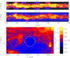 |
Fig. 1 Extinction maps for the inner Galactic plane. Top panel: AKS extinction map, produced using the method of Majewski et al. (2011), covering 342 < l < 352, − 2 < b < +2 deg. Middle panel: EJKS map, produced using the method of Gonzalez et al. (2011a) for the same region (see Sect. 2). Horizontal lines are at b = 0, indicating the Galactic plane, and at |b| = 0.8. Circular areas mark the region around the window and the control field (see Sect. 2). Bottom panel: EJKS map zoomedin the window’s region. The squared and circular areas marked in white are described in Figs. 2 and 3. The horizontal solid line indicates the Galactic plane. The vertical bar shows the colour code for each map. |
2 A new Galactic window
We performed a search for low latitude, low-reddening windows in the Galactic plane using the multi-colour ZY JHKs images and photometry of the disk and bulge fields in the region (− 2.25° < b < 2.25°, 295° < l < 10°) observed by the VVV survey (Saito et al. 2012). We used two different sets of reddening maps that have been independently made. The first reddening map was constructed following the method described in Gonzalez et al. (2011a, 2012), and computed in units of colour excess E(J − KS) (hereafter called “EJKS” map). The latter is based on the Rayleigh–Jeans colour excess method (e.g. Majewski et al. 2011; Nidever et al. 2012) and computed in terms of the total extinction AKs (hereafter “AKS” map). Visual inspection of these maps reveals a window of considerably lower extinction with respect to the neighbouring regions located towards the inner regions of the MW plane at (l, b) = (347.4°, −0.4°) (see Fig. 1). This is the only large region of uniformly low extinction at |b| < 0.8 seen along across all of the maps.
This window can also be seen in the Spitzer Galactic Legacy Infrared Mid-Plane Survey Extraordinaire (GLIMPSE) survey images (Benjamin et al. 2003; Churchwell et al. 2009), in the Planck R2-HFI maps (Planck Collaboration XIX 2011), in the CO maps of Dame et al. (2001) as well as in the density maps of Nidever et al. (2012) and Soto (2013). In all cases, the window can be identified not only in AK values, but also as an enhancement in the number of detected stars. A similar increment in the source density is also seen in the Gaia optical data (Gaia Collaboration 2016).
VVV WIN 1713−3939 has a roughly circular shape of 30′ diameter size, centred at (l, b) = (347.4°, −0.4°) deg. A detailed view of VVV WIN 1713−3939 is presented in Fig. 2. For a Galactic latitude of b = −0.4 deg, the projected vertical height of the line of sight below the Galactic plane at a distance of D = 8 kpc corresponds to z = −56 pc, and at a distance of D = 14 kpc, this height is z = −98 pc, thus making it ideal to trace the properties of the thin disk beyond the Galactic bar.
Reading from the AKS extinction maps, the mean extinction in the window (integrated to a distance of ~10 kpc) is AKs = 0.62 ± 0.07. Reading from the EJKS map, the corresponding mean reddening of the window is E(J − Ks) = 0.96 ± 0.09, which is equivalent to AKs = 0.46 ± 0.04. In general, both maps are in good agreement, however, the AKS maps tend to show higher values than EJKS. A pixel to pixel division (AKS/EJKS map, both in units of AKs) results in a median value of 1.04 ± 0.37 for AKs < 1.2, with larger scatter for increasing AKs values.
A comparison with the maps of Schlegel et al. (1998) and Schlafly & Finkbeiner (2011) reveals that they obtain larger values for the total extinction in this direction, AKs = 1.4 and 1.6, respectively. This systematic difference, in the sense that the AKs in the near-IR is generally lower than the AKs measured inthe far-IR, is seen throughout the Galactic plane regions mapped by the VVV survey.
In order to interpret the colour-magnitude diagrams (CMDs) of VVV WIN 1713−3939 we compare it with a control field located at the same Galactic coordinates, but at the positive latitudes, i.e., centred at (l, b) = (347.4, +0.4) deg (see Fig. 1). The Galactic warp is negligible at these longitudes (e.g. Momany et al. 2006; see their Fig. 9), thus the differences between the control field and the window are expected to be dominated by extinction variation along the line of sight (Δ Ks = 0.5 mag). An examination of the density maps shows a higher density of sources within the window in all VVV filters when compared to the control field. For instance, in Z band which is the filter most affected by extinction, the stellar density in VVV WIN 1713−3939 is 2.7 times larger than that of the control field. There is a similar difference in stellar density observed in the optical Gaia data (Gaia Collaboration 2016). The Gaia source density within the window area is three times larger than the control field. Also, the spatial distribution of the stellar overdensity seen in Gaia is in agreement with the location of the window seen in the extinction and density maps from VVV (see Figs. 2 and 3).
Figure 4 shows as example three HI maps at different velocities, illustrating the relative absence of emission in VVV WIN 1713−3939. The windowin HI suggests a chance superposition of different sizable holes in the near and far side of the tangent point. At the tangent point in l = 347.4 deg (− 185 km s−1), where the HI density is expected to be higher, most of the gas appears to be located above the plane with |b| > 0 deg. The more recent search for Galactic HII regions using Wide-field Infrared Survey Explorer (WISE) data also shows a lack of sources in the low extinction window, and confirms that most known and new candidate HII regions are located above b = 0 deg for this Galactic longitude (Anderson et al. 2014). However, lack of HI on its own does not necessarily mean absence of dust. We note that in this window there is also a lack of integrated CO (1–0 emission line at 115 GHz) in the maps of Dame et al. (2001). For the future, a detailed three-dimensional (3D) comparison with all dust tracers (HI, CO, HII, and dark gas) along the line of sight to this window is needed.
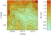 |
Fig. 2 Detailed view of VVV WIN 1713−3939. The map is 36′× 36′ in size, has a resolution of 3′, and corresponds to the squared region marked in Fig. 1. The contour lines show levels of similar E(J − KS), in steps of 0.05 mag. |
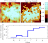 |
Fig. 3 Top: same region of Fig. 2 as seen in the density maps of VVV (Z band) and Gaia (g band), normalised by the maximum value in each case. Vertical bar shows the colour code in the maps. Bottom: total number of sources in the low extinction window divided by the number of sources in the control field for the VVV filters and g band from Gaia. |
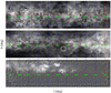 |
Fig. 4 HI maps at different velocities for the inner Galactic plane, for 342.6 < l < 353.4 and − 1.4 < b < 1.4. Top: HI emission for velocities between − 15 and − 20 km s−1. Middle: same for velocities between − 30 and − 42 km s−1. The location of the low extinction window is indicated with the circle. Bottom: same for velocities between − 150 and − 185 km s−1. |
3 The distribution of red clump stars through VVV WIN 1713−3939
Once we have identified the low extinction window, we can explore its stellar content along the line of sight, using RC stars as distance indicators. RC stars are core helium burning giants and excellent distance indicators, and have been used in multiple studies of Galactic structure, in particular those aimed at tracing the bar (e.g. Stanek 1996; Gonzalez et al. 2011a) and the structures towards the inner MW bulge (Nidever et al. 2005; Gonzalez et al. 2012). Also, Benjamin et al. (2005) devised a method to use RC giants from the GLIMPSE survey to investigate the structure of the Galactic plane. This method works well when using GLIMPSE data out to the distance of about 8 kpc (Benjamin et al. 2005), enabling mapping of the near-end of the Galactic bar and nearby spiral arms. However, beyond 8 kpc the GLIMPSE photometry is incomplete (see for example Fig. 5 of Nidever et al. 2012). Alternative distance indicators like variable stars such as RR Lyrae or Cepheids are interesting but of limited use in this case. The RR Lyrae stars represent old metal-poor populations, which are very rare if not absent in the MW disk. In the case of the Cepheids, they represent very young populations, but their surface density is low.
We produce the CMD of VVV WIN 1713−3939 and the control field using the VVV point spread function (PSF) catalogues described in detail in Alonso-García et al. (2015); Alonso-García (2017). One of the immediate advantages of a low extinction window is that it is possible to first inspect the observed CMD, minimising the effects from different assumptions regarding the extinction law in a de-reddened CMD. The Ks versus (J − Ks) CMD for the 30′ diameter window centred at (l, b) = (347.4°, −0.4°) is shown in the left panel of Fig. 5. The observed CMD shows a well-defined double peaked RC feature. We suggest that these are indeed two structures along the line of sight. If this is the case, we expect to observe a jump in extinction from one RC to the other, with each RC getting progressively more reddened, consistent with the larger distances. This is qualitatively what is observed, judging by the CMD shown in Fig. 5.
The observed mean magnitudes and colours for these two RC peaks are Ks, (J − Ks) = 14.07, 1.52 and Ks, (J − Ks) = 14.78, 1.62, respectively.The inspection of the control field shows that only the brighter peak is present. In order to estimate the distances corresponding to the observed magnitudes, we adopt the intrinsic magnitudes and colours of MKs = −1.58 ± 0.03 and (J − Ks) = 0.60 ± 0.01 for the RC following Alves (2002). These magnitudes include the model correction for population effects (relative age and metallicity differences from the Girardi & Salaris (2001) models) with respect to the Large Magellanic Cloud (LMC) where MKs = −1.60 ± 0.03. This is of the same order as the offset found by Pietrzyński & Gieren (2002) between local dwarf galaxies and the MW disk (Δ KsHB = 0.025 mag, their Fig. 7). Furthermore, the mean values for the absolute magnitude of the RC in K band given by different authors agree to within < 0.1 mag (Alves 2000, 2002; Grocholski & Sarajedini 2002; Pietrzyński et al. 2003).
The EJKS reddening map in Fig. 1 traces the integrated extinction along the line of sight, which corresponds to a mean of AKs = 0.46 mag, and E(J − Ks) = 0.95 for VVV WIN 1713−3939. We cannot assume that this reddening is concentrated in any place along the line of sight, although it is probably more severe within the spiral arms. The reddening vector, as measured from the CMD of tile d075 (and adjacent tiles), appears to follow a reddening law slope that is shallower than the traditional Cardelli et al. (1989) value RV = 3.1, shown to be adequate forhigher Galactic latitudes. Therefore, we believe that distances computed using the steep slope from Cardelli et al. (1989; AKs = 0.725 × E(J − Ks)) would be underestimated. We use the method described in Alonso-García (2017) to measure the slope of the reddening vector directly from the CMD as AKs = (0.484 ± 0.040) × E(J − Ks). The slope is measured over all RC stars in the CMD and therefore it is a function only of the specific two-dimensional (2D) location, but does not provide dependence on variations of the extinction law with the distance along the line of sight. This value is similar to AKs = 0.43 × E(J − Ks) measured toward the Galactic centre in Alonso-García (2017), and almost identical to AKs = 0.49 × E(J − Ks) from the recent independent extinction law study by Majaess et al. (2016), obtained from RR Lyrae variables and two separate populations of Cepheids across the entire Galaxy. It is also slightly shallower than the value AKs = 0.528 × E(J − Ks) adopted by Nishiyama et al. (2009).
The RC luminosity function for the window (converted to distance modulus) is shown in the right panel of Fig. 5, along with the data of the comparison field. Adopting the reddening slope measured from the RCs as AKs = 0.484 × E(J − Ks), the distance moduli are computed as μ =−5 + 5 log d(pc) = Ks − 0.484 (J − Ks) + 1.870, following the procedure described by Minniti et al. (2011). We applied a simple Gaussian + polynomial fit in order to obtain the RC mean distances. The distance moduli are μ = 15.20 ± 0.47 and 15.85 ± 0.53, yielding mean RC distances of D = 11.0 ± 2.4 kpc and 14.8 ± 3.6 kpc. For comparison, the distances adopting the relative extinctions (from Catelan et al. 2011) with a slope that follows the Cardelli et al. (1989) reddening law AKs = 0.725 × E(J − Ks) are also presented in Table 1.
The mean errors in the determination of the mean magnitudes for the different features can be derived from the fits to the distribution of distance moduli for the selected red clump stars (Fig. 5). Scaling these errors to the colours according to the reddening slope leads to typical colour uncertainties for the red clumps of σ(J − Ks) = 0.10 mag. We have computed the distances using two different reddening slopes, in order to illustrate that in general the major source of uncertainties is due to the adoption of a specific reddening law, and not from the fits to the RC in the CMD. This is why it is important to make differential distance estimates whenever possible in Galactic plane studies.
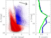 |
Fig. 5 Left: Ks versus (J − Ks) CMD for the circular region around the window as shown in Fig. 1. The blue region was used to derive the RC mags and colours. The contours trace iso density levels. A reddening vector with the slope of AKs = 0.484 × E(J − Ks) is also shown. Right: normalised density distribution of selected RC versus distance moduli of the low extinction window (blue squares) and of the comparison field (green squares). |
Measured magnitudes and colours of the red clump peaks along the line of sight and their derived extinction and distances based on twodifferent extinction laws.
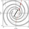 |
Fig. 6 Schematic map of the MW adapted from Vallée (2014) indicating the position of the Sun and the line of sight through the window. We adopted a distance to the Galactic centre of Ro = 8 kpc. According to this picture, the line of sight should pass through the Sagittarius arm and the end of the long bar, and the far side of the Norma and Scutum-Centaurus arms. Red circles mark corresponding distances for the main peaks using AKs = 0.484 × E(J − Ks). Using AKs = 0.725 × E(J − Ks) the distances are systematically shorter (black diamonds). |
4 Mapping distant features in the Galactic disk
The low reddening of VVV WIN 1713−3939 provides us with the opportunity to investigate the entire extension of the disk. Such a study is indeed difficult elsewhere because of the very large extinction at low latitude regions, which introduces severe incompleteness of the main CMDs features. The bottom panel of Fig. 3 illustrates that the number of sources in the window is significantly higher for the relatively bluer passbands.
Figure 6 shows the schematic map of the MW adapted from Vallée (2014), indicating the line of sight towards the window. This picture is in agreement with the schematic face-on view of our Galaxy from Drimmel & Spergel (2001) based on the analysis of near-IR and far-IR data sets. The positions of the RC peaks are also marked.
The most important conclusion from this comparison is that our measured distances match fairly well with those in the graphical representation of the MW. The closest RC, at a mean distance of D = 11.0 kpc (which is also seen in the control field), is consistent with the expected distance to the Galactic bar at this latitude (Wegg et al. 2015). This line of sight intercepts the bar at a projected distance of D ~ 3.5 kpc from the Galactic centre, approximately where the far side of the Sagittarius arm is expected to start.
The second and faintest RC is at D = 14.8 kpc from the Sun and is not seen in the control field luminosity function. A possible interpretation that follows from the comparison in Fig. 6 is that this clump traces the location of the far side of the Norma arm (or even the Scutum–Centaurus arm) along the line of sight, not detected in the control field because of the high extinction. In such a case, the line of sight towards the window intercepts the near side of the Norma arm at a projected distance of about D = 7 kpc from the Galacticcentre. Another possibility is that this peak corresponds to the overall background disk distribution, which would appear narrower due to incompleteness at the faintest magnitudes.
Altogether, our results suggest that VVV WIN 1713−3939 is suitable for studying the overall structure of the disk, potentially tracing important features (such as spiral arms and the general disk density distribution) to constrain our current representation of the far side of the Galaxy. Unfortunately, the choice of the extinction law shrinks or expands the distance scale, but we argue that we have a qualitatively good agreement with the Galactic image of Fig. 6. We note that the Nishiyama et al. (2009); Majaess et al. (2016); or Alonso-García (2017) selective-to-total extinction ratio laws scale better to this picture than steeper options (e.g. Rieke & Lebofsky 1985; Cardelli et al. 1989).
5 Conclusions
We have discovered VVV WIN 1713−3939, a low extinction window in the inner plane of the MW. We show that it is possible to use this window to chart the innermost region of the disk, placing structural constraints on the other side of the Galaxy. In the past our ability to perform such studies using stellar sources has been limited, if not impossible, due to the large amounts of interstellar extinction in the Galactic plane. The new window has a roughly circular shape of 30′ diameter size, centred at (l, b) = (347.4, −0.4) deg. The extinction maps provide a mean extinction of AKs = 0.46 ± 0.04 for this window, corresponding to E(J − Ks) = 0.95, and E(B − V) = 1.45. This is about ΔKs = 0.5 and ΔV = 4.5 mag smaller extinction, on average, than its surrounding fields.
We then studied the stellar populations along the line of sight of this window (and a control field) using the deep near-IR CMDs from the VVV Survey, with the aim of estimating the distances from RC giants, known to be excellent distance indicators. We have computed the slope of the reddening law towards this line of sight, which appears to be shallower than the canonical extinction law of RV = 3.1. We find the slope of the reddening vector is AKs = (0.484 ± 0.040) × E(J − Ks), in agreement with Nishiyama et al. (2009) and more recent studies (Schultheis et al. 2014; Nataf et al. 2016; Majaess et al. 2016; Alonso-García 2017).
Finally, the convenient location of this window allows us to gain a view of the far side of our Galaxy. Using the CMDs we can clearly identify two distant RCs along the line of sight. These stellar over-densities are located at mean distances of D = 11.0 ± 2.4 kpc, and 14.8 ± 3.6 kpc (adopting our measured extinction law, which is similar to that of Nishiyama et al. 2009). These would correspond to the intersection with the Galactic bar and the far Norma (or the far Scutum–Centaurus) arm on the opposite side of the MW, respectively. An alternative interpretation of the most distant RC peak, that it traces the overall background disk population, cannot be excluded. Future studies including proper motion measurements and Cepheid variables to trace over-densities among young stellar populations can further probe the spiral structure of the MW.
Acknowledgements
We gratefully acknowledge the use of data from the ESO Public Survey programme ID 179.B-2002 taken with the VISTA telescope, and data products from the Cambridge Astronomical Survey Unit (CASU). Support for the authors is provided by the BASAL Center for Astrophysics and Associated Technologies (CATA) through grant PFB-06, and the Ministry for the Economy, Development, and Tourism, Programa Iniciativa Cientiífica Milenio through grant IC120009, awarded to the Millennium Institute of Astrophysics (MAS). R.K.S. acknowledges support from CNPq/Brazil through projects 308968/2016-6 and 421687/2016-9. R.K. acknowledges support from CNPq/Brazil. D.M., M.Z., R.B., and J.A.G. acknowledgesupport from FONDECYT Regular grants No. 1130196, 1140076, and 1150345, and Iniciation grant No. 11150916, respectively. We are also grateful to the Aspen Center for Physics where our work was partly supported by National Science Foundation grant PHY-1066293, and by a grant from the Simons Foundation (D.M. and M.R.).
References
- Alonso-García, J., Dekany, I., Catelan, M., et al. 2015, AJ, 149, 99 [NASA ADS] [CrossRef] [Google Scholar]
- Alonso-García, J., Minniti, D., Catelan, M., et al. 2017, ApJ, 849, L13 [NASA ADS] [CrossRef] [Google Scholar]
- Alves, D. 2000, ApJ, 539, 732 [NASA ADS] [CrossRef] [MathSciNet] [Google Scholar]
- Alves, D., Rejkuba, M., Minniti, D., & Cook, K. 2002, ApJ, 573, L51 [NASA ADS] [CrossRef] [Google Scholar]
- Anderson, L. D., Armentrout, W. P., Johnstone, B. M., et al. 2014, ApJS, 212, 1 [NASA ADS] [CrossRef] [Google Scholar]
- Baade, W., & Gaposchkin, C. H. P. 1963, Evolution of Stars and Galaxies (Cambridge, Mass: Harvard University Press), 277 [Google Scholar]
- Benjamin, R. A., Churchwell, E., Babler, B. L., et al. 2003, PASP, 115, 953 [NASA ADS] [CrossRef] [Google Scholar]
- Benjamin, R. A., Churchwell, E., Blaber, B. L., et al. 2005, ApJ, 630, L149 [NASA ADS] [CrossRef] [Google Scholar]
- Cardelli, J. A., Clayton, G. C., & Mathis, J. S. 1989, ApJ, 345, 245 [NASA ADS] [CrossRef] [Google Scholar]
- Catelan, M., Minniti, D., Lucas, P. W., et al. 2011, RR Lyrae Stars, Metal-Poor Stars, and the Galaxy, 5, 145 [NASA ADS] [Google Scholar]
- Churchwell, E., Babler, B. L., Meade, M. R., et al. 2009, PASP, 121, 213 [NASA ADS] [CrossRef] [Google Scholar]
- Dame, T. M., Hartmann, D., & Thaddeus, P. 2001, ApJ, 547, 792 [NASA ADS] [CrossRef] [Google Scholar]
- Drimmel, R., & Spergel, D., 2001, ApJ, 556, 181 [NASA ADS] [CrossRef] [Google Scholar]
- Gaia Collaboration (Brown, A. G. A., et al.) 2016, A&A, 595, A2 [NASA ADS] [CrossRef] [EDP Sciences] [Google Scholar]
- Girardi, L., & Salaris, M. 2001, MNRAS, 323, 109 [NASA ADS] [CrossRef] [Google Scholar]
- Gonzalez, O. A., Rejkuba, M., Minniti, D., et al. 2011a, A&A, 534, L14 [NASA ADS] [CrossRef] [EDP Sciences] [Google Scholar]
- Gonzalez, O. A., Rejkuba, M., Zoccali, M., et al. 2011b, A&A, 530, A54 [NASA ADS] [CrossRef] [EDP Sciences] [Google Scholar]
- Gonzalez, O. A., Rejkuba, M., Zoccali, M., et al. 2012, A&A, 543, 13 [Google Scholar]
- Grenier, I. A., Casandjian, J.-M., & Terrier, R. 2005, Science, 307, 1292 [NASA ADS] [CrossRef] [PubMed] [Google Scholar]
- Grocholski, A.J., & Sarajedini, A. 2002, AJ, 123, 1603 [NASA ADS] [CrossRef] [Google Scholar]
- Jurić, M., Ivezić, Ž, Brooks, A., et al. 2008, ApJ, 673, 864 [NASA ADS] [CrossRef] [MathSciNet] [Google Scholar]
- Majaess, D., et al. 2016, A&A, 593, 124 [Google Scholar]
- Majewski, S. R., Zasowski, G., & Nidever, D. L. 2011, ApJ, 739, 25 [NASA ADS] [CrossRef] [MathSciNet] [Google Scholar]
- McClure-Griffiths, N. M., et al. 2005, ApJS, 158, 178 [NASA ADS] [CrossRef] [Google Scholar]
- Minniti, D., Lucas, P. W., Emerson, J. P., et al. 2010, New Ast., 15, 433 [Google Scholar]
- Minniti, D., Saito, R. K., Alonso-García, et al. 2011, ApJ, 733, L43 [NASA ADS] [CrossRef] [Google Scholar]
- Minniti, D., Saito, R., Gonzalez, O.A., et al. 2014, A&A, 571, A91 [NASA ADS] [CrossRef] [EDP Sciences] [Google Scholar]
- Momany, Y., Zaggia, S., Gilmore, G., et al. 2006, A&A, 451, 515 [NASA ADS] [CrossRef] [EDP Sciences] [Google Scholar]
- Nataf, D. M., Gonzalez, O. A., Casagrande, L., et al. 2016, MNRAS, 456, 2692 [NASA ADS] [CrossRef] [Google Scholar]
- Nidever, D. L., Zasowski, G., & Majewski, S. R. 2012, ApJS, 201, 35 [NASA ADS] [CrossRef] [Google Scholar]
- Nishiyama, S., Nagata, T., Baba, D., et al. 2005, ApJ, 621, L105 [NASA ADS] [CrossRef] [Google Scholar]
- Nishiyama, S., Tamura, M., Hatano, H., et al. 2009, ApJ, 696, 1407 [NASA ADS] [CrossRef] [Google Scholar]
- Pietrzyński, G., & Gieren, W. 2002, AJ, 124, 2633 [NASA ADS] [CrossRef] [Google Scholar]
- Pietrzyński, G., Gieren, W., & Udalski, A. 2003, AJ, 125, 2494 [NASA ADS] [CrossRef] [Google Scholar]
- Planck Collaboration XIX. 2011, A&A, 536, A19 [NASA ADS] [CrossRef] [EDP Sciences] [Google Scholar]
- Reid, M. J., Menten, K. M., Zheng, X. W., et al. 2009, ApJ, 700, 137 [NASA ADS] [CrossRef] [Google Scholar]
- Rieke, G. H., & Lebofsky, M. J. 1985, ApJ, 288, 618 [NASA ADS] [CrossRef] [Google Scholar]
- Saito, R. K., Hempel, M., Minniti, D., et al. 2012, A&A, 537, A107 [NASA ADS] [CrossRef] [EDP Sciences] [Google Scholar]
- Schlafly, E. F., & Finkbeiner, D. P. 2011, ApJ, 737, 103 [NASA ADS] [CrossRef] [Google Scholar]
- Schlegel, D. J., Finkbeiner, D. P., & Davis, M. 1998, ApJ, 500, 525 [NASA ADS] [CrossRef] [Google Scholar]
- Schultheis, M., Chen, B. Q., Jiang, B. W., et al. 2014, A&A, 566, 120 [Google Scholar]
- Soto, M., Barbá, R., Gunthardt, G., et al. 2013, A&A, 552, A101 [NASA ADS] [CrossRef] [EDP Sciences] [Google Scholar]
- Stanek, K. Z. 1996, ApJ, 460, L37 [NASA ADS] [CrossRef] [Google Scholar]
- Vallée, J. P. 2014, ApJS, 215, 1 [CrossRef] [Google Scholar]
- Vallée, J. P. 2017, Astron. Rev., 13, 113 [CrossRef] [Google Scholar]
- Wegg, C., & Gerhard, O. 2013, MNRAS, 435, 1874 [Google Scholar]
- Wegg, C., Gerhard, O., & Portail, M. 2015, MNRAS, 450, 4050 [NASA ADS] [CrossRef] [Google Scholar]
All Tables
Measured magnitudes and colours of the red clump peaks along the line of sight and their derived extinction and distances based on twodifferent extinction laws.
All Figures
|
Fig. 1 Extinction maps for the inner Galactic plane. Top panel: AKS extinction map, produced using the method of Majewski et al. (2011), covering 342 < l < 352, − 2 < b < +2 deg. Middle panel: EJKS map, produced using the method of Gonzalez et al. (2011a) for the same region (see Sect. 2). Horizontal lines are at b = 0, indicating the Galactic plane, and at |b| = 0.8. Circular areas mark the region around the window and the control field (see Sect. 2). Bottom panel: EJKS map zoomedin the window’s region. The squared and circular areas marked in white are described in Figs. 2 and 3. The horizontal solid line indicates the Galactic plane. The vertical bar shows the colour code for each map. |
| In the text | |
|
Fig. 2 Detailed view of VVV WIN 1713−3939. The map is 36′× 36′ in size, has a resolution of 3′, and corresponds to the squared region marked in Fig. 1. The contour lines show levels of similar E(J − KS), in steps of 0.05 mag. |
| In the text | |
|
Fig. 3 Top: same region of Fig. 2 as seen in the density maps of VVV (Z band) and Gaia (g band), normalised by the maximum value in each case. Vertical bar shows the colour code in the maps. Bottom: total number of sources in the low extinction window divided by the number of sources in the control field for the VVV filters and g band from Gaia. |
| In the text | |
|
Fig. 4 HI maps at different velocities for the inner Galactic plane, for 342.6 < l < 353.4 and − 1.4 < b < 1.4. Top: HI emission for velocities between − 15 and − 20 km s−1. Middle: same for velocities between − 30 and − 42 km s−1. The location of the low extinction window is indicated with the circle. Bottom: same for velocities between − 150 and − 185 km s−1. |
| In the text | |
|
Fig. 5 Left: Ks versus (J − Ks) CMD for the circular region around the window as shown in Fig. 1. The blue region was used to derive the RC mags and colours. The contours trace iso density levels. A reddening vector with the slope of AKs = 0.484 × E(J − Ks) is also shown. Right: normalised density distribution of selected RC versus distance moduli of the low extinction window (blue squares) and of the comparison field (green squares). |
| In the text | |
|
Fig. 6 Schematic map of the MW adapted from Vallée (2014) indicating the position of the Sun and the line of sight through the window. We adopted a distance to the Galactic centre of Ro = 8 kpc. According to this picture, the line of sight should pass through the Sagittarius arm and the end of the long bar, and the far side of the Norma and Scutum-Centaurus arms. Red circles mark corresponding distances for the main peaks using AKs = 0.484 × E(J − Ks). Using AKs = 0.725 × E(J − Ks) the distances are systematically shorter (black diamonds). |
| In the text | |
Current usage metrics show cumulative count of Article Views (full-text article views including HTML views, PDF and ePub downloads, according to the available data) and Abstracts Views on Vision4Press platform.
Data correspond to usage on the plateform after 2015. The current usage metrics is available 48-96 hours after online publication and is updated daily on week days.
Initial download of the metrics may take a while.