| Issue |
A&A
Volume 616, August 2018
|
|
|---|---|---|
| Article Number | A22 | |
| Number of page(s) | 13 | |
| Section | Extragalactic astronomy | |
| DOI | https://doi.org/10.1051/0004-6361/201731712 | |
| Published online | 07 August 2018 | |
Evidence for the formation of the young counter-rotating stellar disk from gas acquired by IC 719★,★★
1
Dipartimento di Fisica e Astronomia “G. Galilei”, Università di Padova,
vicolo dell’Osservatorio 3,
35122
Padova, Italy
e-mail: This email address is being protected from spambots. You need JavaScript enabled to view it.
2
INAF - Osservatorio Astronomico di Padova,
vicolo dell’Osservatorio 5,
35122
Padova, Italy
3
European Southern Observatory,
Karl-Schwarzschild-Strasse 2,
85748
Garching, Germany
4
Max-Planck-Institut für extraterrestrische Physik,
Giessenbachstrasse,
85748
Garching, Germany
5
Universitäts-Sternwarte München,
Scheinerstrasse 1,
81679
München, Germany
Received:
4
August
2017
Accepted:
28
March
2018
Abstract
Aims. The formation scenario of extended counter-rotating stellar disks in galaxies is still debated. In this paper, we study the S0 galaxy IC 719 known to host two large-scale counter-rotating stellar disks in order to investigate their formation mechanism.
Methods. We exploit the large field of view and wavelength coverage of the Multi Unit Spectroscopic Explorer (MUSE) spectrograph to derive two-dimensional (2D) maps of the various properties of the counter-rotating stellar disks, such as age, metallicity, kinematics, spatial distribution, the kinematical and chemical properties of the ionized gas, and the dust map.
Results. Due to the large wavelength range, and in particular to the presence of the Calcium Triplet λλ8498, 8542, 8662 Å (CaT hereafter), the spectroscopic analysis allows us to separate the two stellar components in great detail. This permits precise measurement of both the velocity and velocity dispersion of the two components as well as their spatial distribution. We derived a 2D map of the age and metallicity of the two stellar components, as well as the star formation rate and gas-phase metallicity from the ionized gas emission maps.
Conclusions. The main stellar disk of the galaxy is kinematically hotter, older, thicker and with larger scale-length than the secondary disk. There is no doubt that the latter is strongly linked to the ionized gas component: they have the same kinematics and similar vertical and radial spatial distribution. This result is in favor of a gas accretion scenario over a binary merger scenario to explain the origin of counter-rotation in IC 719. One source of gas that may have contributed to the accretion process is the cloud that surrounds IC 719.
Key words: galaxies: individual: ic 719 / galaxies: kinematics and dynamics / galaxies: stellar content / galaxies: formation
Based on observation collected at the European Southern Observatory for the programme 095.B-0686(A).
The reduced datacube is only available at the CDS via anonymous ftp to cdsarc.u-strasbg.fr (130.79.128.5) or via http://cdsarc.u-strasbg.fr/viz-bin/qcat?J/A+A/616/A22
© ESO 2018
1 Introduction
It is widely accepted that galaxies undergo a number of acquisition events during their evolution and growth. Depending on the nature of the accreted material and on the geometry of the process, such events may leave temporary or permanent signatures on the morphology, kinematics, and stellar population properties of the host galaxy. Among these, the presence of structural components with remarkably different kinematics represents a fascinating case. A large variety of phenomena enters in this category, such as counter-rotating gas disks (Ciri et al. 1995; Chung et al. 2012), counter-rotating stellar disks (Rubin et al. 1992; Bertola et al. 1996), orthogonal bulges (Bertola et al. 1999; Sarzi et al. 2001; Corsini et al. 2012), orthogonal gaseous structures (Corsini et al. 2002), and decoupled stellar cores (Sarzi et al. 2000); see Galletta (1996), Bertola & Corsini (1999), and Corsini (2014) for reviews.
In this paper, we investigate the case of extended counter-rotation of large stellar disks. Although some attempts have been made to explain stellar counter-rotation as due to self-induced phenomena, such as dissolving bars (e.g., Evans & Collett 1994), this phenomenon is usually considered as the signature of a past merging event or accretion (e.g., Thakar et al. 1997; Algorry et al. 2014; Bassett et al. 2017). However, the details of the formation mechanisms of large counter-rotating stellar disks are still under debate, and their existence still represents a puzzle in the broad context of formation and evolution of galaxies.
In the current theoretical picture, two scenarios have been proposed to explain their formation, each leaving different signatures in the kinematics and stellar populations: i) binary galaxy major mergers (e.g., Puerari & Pfenniger 2001); and ii) gas accretion or gas-rich minor mergers on a pre-existing galaxy followed by star formation (e.g., Thakar & Ryden 1998; Bassett et al. 2017).
A major merger of two disk galaxies may end up with the formation of a disk galaxy with a massive counter-rotating disk under certain conditions. Crocker et al. (2009) built a numerical simulation to explain the case of NGC 4550. They found that two gas-rich disk galaxies of similar mass can merge and, depending on the geometry of the encounter, can form a massive disk galaxy with two counter-rotating stellar disks embedded one into the other. Concerning the fate of the gas component, the more prominent one, after dissipating with its counter-rotating counterpart, settles onto the equatorial plane. The two resulting disks have different thicknesses, the one associated to the gas being dynamically hotter than the other. In this scenario, the stellar population properties of the two stellar components depend on the properties of the progenitors and on star-formation episodes triggered by the merger itself. On the other hand, this result holds for this specific case of a perfectly co-planar merger, and other possibilities should be investigated too.
When a gas-poor disk galaxy acquires gas from the surrounding environment (either in a short or prolonged episode) or from a gas-rich minor merger, a counter-rotating stellar disk may form if the gas angular momentum is opposite to that of the host galaxy. The newly-formed counter-rotating stellar disk is thinner and dynamically colder than the prograde disk. The spatial distribution of the counter-rotating component depends on the initial angular momentum of the acquired gas and on the amount of gas in theprimordial galaxy. In this scenario, the stellar component associated to the gas disk is predicted to be the youngest. Moreover, if the secondary stellar disk has formed recently, it is expected to have similar metallicity to the gas from which it originated. The analysis of the metallicity of both the stellar and gas-phase components can be used to identify the gas reservoir that formed the prograde and/or retrograde stellar components (Coccato et al. 2013). Algorry et al. (2014) considered the case where gas is acquired in a single episode and found that it may give rise to two counter-rotating stellar disks with different scale lengths and significantly different ages. A similar result is found by Bassett et al. (2017) simulating a 1:10 minor merger between a gas-poor galaxy and a less-massive gas-rich one.
One key aspect in this investigation is to study the counter-rotating components independently by removing their mutual contamination on the total observed spectrum along the line of sight (LOS). Indeed, in recent years we have developed a spectroscopic decomposition technique that fits the kinematics and the stellar populations of two stellar components, and therefore separates their contribution from the total observed spectrum (Coccato et al. 2011). The spectroscopic decomposition technique is particularly suitable in the study of extended counter-rotating disks where the LOS velocity of the two stellar components and their low velocity dispersion allows a reliable spectroscopic separation. It has been further developed and successfully applied by several teams to a number of disk galaxies with stellar counter-rotation: NGC 524 (Katkov et al. 2011), IC 719 (Katkov et al. 2013), NGC 448 (Katkov et al. 2016), NGC 1366 (Morelli et al. 2017), NGC 3593 (Coccato et al. 2013), NGC 4138 (Pizzella et al. 2014), NGC 4191 (Coccato et al. 2015), NGC 4550 (Coccato et al. 2013; Johnston et al. 2013), NGC 5102 (Mitzkus et al. 2017), and NGC 5719 (Coccato et al. 2011). The technique was also applied to study orthogonally decoupled structures such as polar rings (Coccato et al. 2014) and photometrically distinct components such as bulge and disk (Fabricius et al. 2014; Tabor et al. 2017).
A lot of importance was given to the age and metallicity of the two stellar components, and to the gas-phase metallicity in order to identify the most probable formation scenario. In most cases, a significant difference in the age of the stellar population of the two components was found. The younger stellar component was always found to be co-rotating with the gaseous disk, and to be the least luminous and least massive. This supports the gas accretion scenario, although without totally excluding the binary merging scenario.
Few exceptions are found to this picture. In NGC 4550 and NGC 448, the two counter-rotating stellar disks have similar ages. It is interesting to note that they are the oldest systems analyzed to date, with T ~ 7 Gyr and T ~ 9 Gyr, respectively. The most intriguing exception is NGC 1366. In this galaxy, the ionized gas component is not kinematically associated to either of the stellar counter-rotating components. The most plausible interpretation is that the gas clouds are still in chaotic motion, possibly dissipating to a disk at present (Morelli et al. 2017). The ambiguity of the results on NGC 1366 suggests that additional physical properties are needed to establish a direct link between the ionized-gas disk and the secondary counter-rotating stellar component, in addition to the velocity and stellar population properties of the two components.
For this reason, in this paper we take into account other physical quantities that play a relevant role in the analysis of such complex systems in addition to the previous analyzed observables. One of these is the velocity dispersion of the stellar components. Qu et al. (2011) show that, if the counter-rotating stellar disk recently formed from the gaseous disk as a consequence of a gas-rich minor merger, we expect that such a newly formed disk is characterized by a low velocity dispersion and a flattening which should be similar to those of the gaseous disk. On the contrary, an older stellar disk should be thicker and have a larger velocity dispersion due to dynamical heating processes (e.g., Gerssen & Shapiro Griffin 2012). In this case, the counter-rotating gaseous disk is the result of a subsequent acquisition event. This seems to be the case for explaining the formation of the counter-rotating disk in NGC 1366 (Morelli et al. 2017).
Another important constraint to firmly link the stellar and gas disks is the present-day star formation activity. If the stellar disk is still currently forming stars, the consequent star formation should be evident in the spectra. In some of the targets, we did find active star formation arranged in a ring-like structure of kiloparsec scale (NGC 3593, NGC 4138, and NGC 5719). The knowledge of its location and strength gives important clues about the timing of the formation process as star formation is the process that transforms the gas into stars.
The recent construction of integral field unit spectrographs characterized by a large field of view and extended wavelength range gives the possibility of a step forward in the study of these objects. In particular the Multi Unit Spectroscopic Explorer (MUSE; Bacon et al. 2010) operating on the Very Large Telescope (VLT) allows us to map counter-rotating galaxies with an unprecedented efficiency in terms of telescope time, due to the combination of a large field of view and high optical efficiency. In addition, the spectral resolution that characterizes MUSE in the CaT wavelength region allows one to clearly separate these absorption lines as soon as the difference in velocity of the two stellar components is greater than ~ 50 km s−1. In the most favorable cases, we can measure not only the velocity but also the velocity dispersion of the two stellar disks. This allows us to compare the velocity dispersion of the stellar and gas disk to obtain crucial constraints on their connections and formation.
In this work we study the early-type disk galaxy IC 719 (Fig. 1). It is classified as S0? by de Vaucouleurs et al. (1991, hereafter RC3), and its apparent size and magnitude are 0.′65 × 0.′20 and  mag (RC3). The disk inclination is i = 77° derived from the ring-like structure visible in the near-infrared (NIR) bands as shown by Katkov et al. 2013. This structure is very well spatially defined and represents the best indicator of galaxy inclination. The galaxy is therefore well spatially resolved and relatively bright, two necessary conditions to conduct our analysis. In this work we adopt a photometric position angle in the sky of PA = 53° (counted from North to East) and a distance to the galaxy of D = 28.6 Mpc (from the NASA/IPAC extragalactic database).
The galaxy is known to have an extended counter-rotating stellar component and was studied by Katkov et al. (2013) by means of long-slit and SAURON integral field spectroscopy. It therefore represents an ideal target to be re-observed with the capabilities of the MUSE integral field spectrograph. With our new observations, in particular with the aid of an extended field of view and wavelength coverage, we are able to improve the accuracy and precision on the observables and measure with great precision the properties (kinematics, morphology, and stellar population) of the two stellar disks, the star formation rate (SFR), and the gas-phase metallicity.
This paper is organized as follows. The observations and data reduction are presented in Sect. 2. In Sect. 3 we describe the data analysis. The results about the measurements of the distribution, kinematics, and chemical properties of the stars and ionized gas are given in Sect. 4. We discuss our results and present our conclusions in Sect. 5.
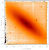 |
Fig. 1 MUSE image of IC 719. The image was obtained by averaging the wavelength range 7500–8000 Å. The image intensity is shown with a logarithmic scale. The field of view and orientation of all 2D maps of the paper are ~ 1′ × 1′ and north up, east left. |
2 Observations and data reduction
The observations of IC 719 were carried out in service mode at European Southern Observatory (ESO) in Cerro Paranal with the UT4-Yepun telescope equipped with MUSE on April 11, 2015. The chosen setup was the nominal mode which delivers a wavelength range of 4800–9300 Å with a resolving power ranging from 1770 at 4800 Å to 3590 at 9300 Å. Spectral sampling is of 1.25 Åpixel−1 while the spatial sampling is 0. ′′2 × 0. ′′2 pixel−2. The field of view is 1′ × 1′.
The target was acquired in the center of the instrument field of view. The total integration was split into three different exposures of 840 s each. An offset of 1′′ and a rotation of 90° was applied between each exposure in order to properly address spatial instrumental inhomogeneities. A sky exposure of 300 s was taken during the same observing block with an offset of about 100′′ with respect to the galaxy center parallel to its minor axis in a sky region free of bright stars.
2.1 Data reduction
The raw data from each exposure were pre-reduced and combined with the MUSE pipeline v1.4 muse/1.1.90 (Weilbacher et al. 2012)run under the EsoReflex environment (Freudling et al. 2013). The reduction includes bias subtraction, flat-fielding, and illumination correction (using a twilight exposure), wavelength calibration, and alignment and a combination of the three exposures. One standard star was observed at the beginning of the night that we used for flux calibration and correction of telluric features. The contribution of the night sky has been removed from the spectra by the data reduction pipeline using the offset sky exposure.
The seeing FWHM read from the ESO seeing monitor was in the range 1. ′′ 0 < FWHM < 1. ′′5 during the observations, consistent with the value of FWHM = 1. ′′3 measured on bona-fide unresolved HII regions visible in the final combined datacube. We used a sky spectrum, extracted from the datacube before sky subtraction, to check the spectral resolution. The spectra of about 1000 spaxels have been averaged in a region free of galaxy contamination and we performed a Gaussian fit on the night sky emission lines. The central wavelength and FWHM of ~ 140 lines were obtained and compared with the line atlas from Osterbrock et al. (1996, 1997). We found mean offset of λmeasure − λsky = −0.40 ± 0.09 Å constant with wavelength. The FWHM shows some variation at different wavelengths, being 2.65 ± 0.08 Å at H β, 2.50 ± 0.08 Å at H α, and 2.39 ± 0.08 Å in the CaT region. This is in very good agreement with the nominal values of the instrument (Bacon et al. 2010). The resulting instrumental velocity dispersion is 69.4 ± 2.1 km s−1 at H β, 48.5 ± 1.5 km s−1 at H α, and 35.3 ± 1.2 km s−1 in the CaT region.
2.2 Spatial re-sampling of the data cube
After pre-reduction we averaged the one-dimensional (1D) spectra of adjacent single spaxels in order to increase the signal-to-noise ratio (S/N) of the resulting 1D spectra. We used the adaptive spatial binning software developed by Cappellari & Copin (2003) based on Voronoi tessellation. We estimated the signal of each individual spaxel by taking the median of the flux in the wavelength range 4762–6737 Å, which is thelargest range avoiding the spectral region more effected by atmospheric absorption and emission features.
We chose a target S/N of 120 in each bin. As noise we adopted the square root of the median of the variancegiven by the pipeline. It must be noted that this is not the S/N of the binned spectra. The latter is estimated a posteriori from the residual fitting the galaxy spectra and turned out to be ~ 40.
We obtained 144 independent spectra. In the center of the galaxy, where the signal is higher, the area covered by each bin is about 1′′ × 1′′ (~ 25 pixels) while in more external regions it can be up to about 4′′ × 4′′ (~ 400 pixels).
2.3 Optimization of the sky subtraction
Some residual sky emission was still present at the end of pre-reduction. We therefore performed a further correction as follows. We took theaverage of all the single spectra with absent or very low signal that for this reason were discarded when building the spatially binned Voronoi tessellation. We took this average spectrum as a template for the “sky-residual”. We then subtracted this template from each of the 144 spectra after scaling it with a proper factor chosen to reduce the scatter in regions free of strong galaxy features but with a relevant residual of the first sky subtraction above 7500 Å. The result is a clean spectrum. Spectral regions affected by relevant sky lines were nonetheless masked when analyzing the spectra (Sect. 3).
3 Analysis
3.1 Stellar and ionized gas kinematics
We measured the kinematics of the two stellar components and of the ionized gas using the implementation of the penalized pixel fitting code (pPXF, Cappellari & Emsellem 2004) developed by Coccato et al. (2011). In each spatial bin, the code builds the spectrum of the galaxy as the combination of two synthetic templates, one for each stellar component. The single template is built as the linear combination of stellar spectra from the library of Munari et al. (2005), characterized by an instrumental FWHM = 1.35 Å, for the CaT region, and the extended Medium-resolution INT Library of Empirical Spectra library (MILES) with the canonical base models BaseFe Vazdekis et al. (2012), with instrumental FWHM = 2.54 Å (Beifiori et al. 2011; Falcón-Barroso et al. 2011) when considering the whole spectral range. The template is convolved with Gaussian line-of-sight velocity distributions (LOSVDs). The LOSVDs used for the two stellar components have different velocities and velocity dispersions. Spectra are normalized to their continuum level at 5100 Å, therefore the relative contribution of each component to the total spectrum is in terms of light. Gaussian functions are added to the involved synthetic templates to account for ionized-gas emission lines and fit simultaneously to the observed galaxy spectra. Multiplicative Legendre polynomials are included in the fit for both synthetic templates to match the shape of the galaxy continuum. The use of multiplicative polynomials also accounts for the effects of dust extinction and variations in the instrument transmission. As a result of the fit, for each spatial bin, the code returns the spectra of the two best-fit synthetic stellar templates and ionized-gas emissions, along with their best-fitting parameters: Fr (that we define as the ratio between the flux of one component and the total flux), velocity, and velocity dispersion. Errors on all parameters are computed by the modified pPXF routine as in Cappellari & Emsellem (2004). The line strength of the Lick indices of the two counter-rotating components are measured from the two best-fit synthetic templates. A number of wavelength regions were masked out when performing the fit because they are affected by poor sky subtraction. Also, regions with no relevant stellar absorption features were masked in order to increase the effective S/N. The procedure was applied in two steps, considering two different spectral ranges. The wavelength range 8500–8800 Å, which contains prominent Ca absorption-line features, was used to gain a precise measurement of the kinematics. In fact, the MUSE resolving power is higher at this wavelength range (σ8600 Å ~ 35 km s−1) than in the Mg range (σ5200 Å ~ 60 km s−1). Thus, we better resolve the absorption line features and obtain more precise measurements of velocity and, in particular, velocity dispersion of the two stellar components, by measuring the kinematics in the CaT region. This is why we adopted the library stellar by Munari et al. (2005) in this spectral region. In Fig. 2 we plot an example of the spectral decomposition in a bin positioned along the major axis of the galaxy where the two components are well separated. The best fit velocity and velocity dispersion measured in the CaT region were used as starting guesses to fit the spectra in the full 4778–9200 Å wavelength range (Fig. 3). The best fit spectra obtained in this range were used to measure the ionized-gas kinematics and intensity, and the luminosity fraction of the two components. In Fig. 3 we show the best fit to the full wavelength range obtained for the same spatial bin as in Fig. 2. To measure the stellar population properties, we repeated the spectral fit considering only the 4778–5450 Å wavelength range. In this case, we kept the velocity and velocity dispersion fixed to the values measured in the CaT region and left all the other parameters free to vary. In Fig. 4 we show the result for the same spatial bin as in Fig. 2.
After having measured all bins, we sort the two components using their velocity. We define the main component to be the stellar component which is receding on the NE side of the plane of the sky (and therefore approaching on the SW side). This turned out to be the most luminous component. We define the secondary component to be the other stellar component. The decomposition is more robust in those spatial bins where the velocity separation is high and the luminosity of the two components is similar. We consider the two stellar components to be “kinematically separated” if their velocity separation is higher than 50 km s−1, and 0.15 < Fr < 0.85. The spatial bins where we could not separate the two components identify a circular region with radius ~5′′ from the center and a conic region aligned along the minor axis. Consequently, the spatial bins in which the stellar components can be considered as kinematically separated identify a conic region aligned with the galaxy major axis. From now on, although we fit the kinematics on the whole galaxy, we consider only spatial bins with the spectra of the two components well separated. Furthermore, we consider the whole galaxy only concerning the ionized gas emissions. This choice minimizes issues related to degeneracies in the spectral decomposition code (e.g., if two components have the same velocity, thestellar templates used to determine the best fit can be assigned to one component or the other without changing the best fitting model), and the contamination of the galaxy bulge, which is confined in the innermost ~3′′ (see Fig. 1 in Katkov et al. 2013). In Figs. 5 and 6 we show the velocity and velocity dispersion 2D fields of the two stellar and ionized gas components, as measured in the CaT spectral region.
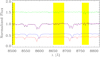 |
Fig. 2 Example of the observed (black line) and fitted spectrum in a bin where the two stellar components appear separated. Here the fit is limited to the CaT wavelength region. We show the two stellar spectra fitted to the data (blue and red lines), and their sum (magenta line). The green line represents the residuals shifted upward by 1.5 units. The yellow regions are regions masked and not included in the fit. |
3.2 Emission line maps
After having derived the ionized gas velocity field, we extracted the emission line maps of all the emission lines present in the spectral range. The spectral lines, some of which were not included in the kinematical fit, are H β, [O III] λλ4959, 5007, [N II] λλ5198, 5200, [He I], λ5875, [O I] λλ6300, 6363, [N II] λλ6548, 6583, H α, [He I], λ6678, [S II] λλ6716, 6731, and [ArI], λ7135. We do this on the unbinned datacube in order to draw maps with the original spatial sampling of the instrument. At each spaxel of the unbinned datacube, we subtract the stellar best-fitting spectrum of the Voronoi bin belonging to that specificspaxel. The stellar model spectrum was scaled by a factor that was chosen such that it matches the stellar continuum. The wavelength of the emission line is computed from the ionized gas velocity measured in the same Voronoi bin. Subsequently, for each spaxel, the emission line flux is obtained by integrating the signal of an 11 Å-wide wavelength region centered on the line. The width of 11 Å was used in order to include all the flux of the line and to avoid contamination from the nearby emission lines. This produces an emission line map with a spatial sampling of 0. ′′2. Examples of the four main emission-line maps are shown in Fig. 8.
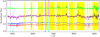 |
Fig. 3 As in Fig. 2 but considering the whole wavelength extension. The cyan line represents the ionized gas emissionwhile the magenta line represents the sum of the two stellar components and the ionized gas emission. |
3.3 Line-strength indices
We measured the Lick indices on the best fit spectra obtained in the spectral fit (Fig. 4, blue and red lines). We show in Figs. 9 and 10 the 2D maps of the equivalent width (EW) of the H β, Mgb, Fe5270, and Fe5335 absorption lines. The combined magnesium-iron index ![Mathematical equation: $[\textrm{MgFe}]^{\prime}=\sqrt{\textrm{Mg}\,b\,\left(0.72\times {\textrm{Fe5270}} + 0.28\times{\textrm{Fe5335}}\right)}$](/articles/aa/full_html/2018/08/aa31712-17/aa31712-17-eq2.png) (Thomas & Maraston 2003) and the average iron index
⟨Fe⟩ = (Fe5270 + Fe5335)/2 were computed too. Errors on indices were derived from photon statistics and CCD readout noise, and calibrated by means of Monte Carlo simulations (Morelli et al. 2012, 2016). In Fig. 11, we compare the measured line-strength indices to the prediction of simple stellar population models by Thomas et al. (2011). The two stellar components occupy different areas of the diagnostic plots of Fig. 11 and show a wide range of metallicities and ages.
(Thomas & Maraston 2003) and the average iron index
⟨Fe⟩ = (Fe5270 + Fe5335)/2 were computed too. Errors on indices were derived from photon statistics and CCD readout noise, and calibrated by means of Monte Carlo simulations (Morelli et al. 2012, 2016). In Fig. 11, we compare the measured line-strength indices to the prediction of simple stellar population models by Thomas et al. (2011). The two stellar components occupy different areas of the diagnostic plots of Fig. 11 and show a wide range of metallicities and ages.
4 Results
The spectraldecomposition successfully identified the presence of two stellar components in IC 719 (Figs. 2 and 3). We determined the rotation curves and the velocity dispersion radial profiles (Sect. 4.1) and the stellar populations of the two components (Sect. 4.3). In Sect. 4.2, we reconstruct the images of the two stellar disks and study their morphology; in Sect. 4.5, we use the measured emission lines to derive the spatially resolved SFR.
4.1 Kinematics
The spectral decomposition confirmed the presence of two extended stellar components in IC 719 that rotate in opposite directions, as shown in Fig. 5. The larger the velocity difference, the clearer the separation between the absorption lines of the two stellar components. The double-peaked feature of the absorption lines is particularly evident in the CaT region, where the instrumental velocity resolution is better than in the Mg region (Figs. 2 and 4). In comparison with previous works based on the Mg region, the use of the CaT not only allows a more precise determination of the velocity, butalso a more reliable measurement of the velocity dispersion, which is important to infer the formation scenario (see Sect. 5).
The main stellar component, which is the one receding in the NE side of the galaxy, reaches a rotation of ± 150 km s−1 at about 2 kpc from the galaxy center and has an almost constant rotation velocity out to the outermost observed bin (≈ 3 kpc). Its velocity dispersion ranges from ~ 70 km s−1 in the most central radius we could measure (0.5 kpc) to ~ 50 km s−1 in the outermost regions. The secondary stellar component rotates in the opposite direction, and is characterized by a slightly steeper velocity gradient and higher rotation amplitude: 180 km s−1 reached at ≈2 kpc from the galaxy center. The secondary stellar component is kinematically colder than the main component, with a velocity dispersion that ranges between 50 km s−1 at ~ 0.5 kpc and 30 km s−1 in the outer regions, a value smaller than the instrument velocity resolution.
The ionized gas rotates along the same direction as the secondary stellar component; its rotation amplitude and radial profile of the velocity dispersion are similar to those of the secondary stellar component (Fig. 7).
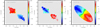 |
Fig. 5 Velocity field of the main component (left panel), secondary component (center panel), and of the ionized gas component (right panel). Typical errors are 7 km s−1 for the stellar components and 2 km s−1 for the ionized gas. |
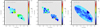 |
Fig. 6 As in Fig. 5 for the velocity dispersion field. Typical errors are 10 km s−1 for the stellar components and 2 km s−1 for the ionized gas. |
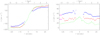 |
Fig. 7 Velocity (left panel) and velocity dispersion curve (right panel) extracted along the major axis of IC 719. Blue, red, and green lines represent the main stellar component, secondary stellar component, and ionized gas, respectively. The velocity of the main component has been changed in sign in order to allow a direct comparison with the velocity of the other two components. The instrumental velocity dispersion of 35 km s−1 (CaT) and 53 km s−1 (Hα ) is indicated as reference by a horizontal tick. The extraction of the kinematics along the major axis has been doneby spatial averaging the spaxels in Figs. 5 and 6 considering a 2′′ -wide aperture passing thought the center along PA = 53°. Typical error-bars on the velocity and velocity dispersion are 5 and 10 km s−1, respectively. |
4.2 Morphology of the stellar disks
We derive the 2D light distributions of the two stellar disks, their surface brightness profiles, and their relative flux contributions from the Fr measured at each spatial bin by the spectral decomposition code and the galaxy image (Fig. 12). We applied the same Voronoi binning used for the kinematical analysis to the reconstructed image of IC 719. We then obtained the image of the primary stellar component by multiplying it by the Fr map (or the secondary component by multiplying it by 1 − Fr). Figure 13 shows the reconstructed images of the two stellar components. We can then derive the radial surface brightness profile of both stellar components (Fig. 14). This is done using the task ellipse of the IRAF1. The main component has an exponential profile with scale length of ~ 1.5 kpc; the secondary component follows an exponential profile with a possible truncation beyond 4 kpc. Its scale length is ~1 kpc and therefore smaller than the primary disk. We also used the reconstructed images to derive the isophotal shape at different radii of the two stellar components. Because of the limited number of data points, we first created a regular square matrix of pixels with the same size as the MUSE field of view. We assigned to each pixel the corresponding flux value belonging to that Voronoi bin. We then fitted ellipses with fixed center and position angle to this frame. The result is plotted in Fig. 14.
Both the main and secondary components contribute (50 ± 15)% of the stellar luminosity at about 1.0 kpc, while the main component dominates in the outer regions of the galaxy being (65 ± 15)% at about ≃ 2.5 kpc, and (85 ± 15)% at about ≃ 6.0 kpc. In total, the secondary component contributes to 35% of the galaxy light as measured from 0.8 to 4.2 kpc.
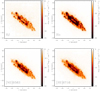 |
Fig. 8 Emission line maps, from top left to bottom right panel, for Hβ, H α, [N II] λ6583, and [S II] λ6716. The field of view is 1′× 1′. N is up and E is left. |
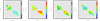 |
Fig. 9 Equivalent width map of the main component for the Hβ, Mgb, Fe5270, and Fe5335 absorption lines. The color indicates the EW in each bin as indicated by the color bar. The field of view is 1′ × 1′. N is up and E is left. |
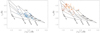 |
Fig. 11 Lick indices for the main component (left panel, blue dots) and the secondary component (right panel, red dots). The color tonality indicates the position of the measurement with lighter colors for the central regions and darker colors for the external regions. The lines are the loci of constant age and metallicity as indicates by the labels. |
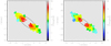 |
Fig. 12 Luminosity fraction of the secondary component over the total, as a function of radius. |
4.3 Stellar populations
For each binwe derived the map of the luminosity-weighted age and metallicity of both the stellar components by comparing the measurements of the line-strength indices Hβ, Mgb, [MgFe]’, and ⟨Fe⟩ with the model predictions by Thomas et al. (2011) for a single stellar population. In this parameter space the mean age and metallicity appear to be almost insensitive to the variations of the α∕Fe enhancement. Age and metallicities were derived by linear interpolation between the model points using the iterative procedure described in Mehlert et al. (2003). The final result is a 2D map of age and metallicity for both the stellar components (Fig. 15).
The ageand metallicity of both stellar components depend on the distance from the galaxy center. In order to analyze them we extracted their radial profiles from the 2D maps as follows.
For eachpoint in the field of view, we computed the deprojected distance from the center of the galaxy assuming a disk major axis in the sky at PA = 53°, and the inclination of 77°. We then averaged age and metallicity values falling in the same deprojected radial bins. The results are shown in Fig. 16.
We find that the primary component has a luminosity-weighted age of about 3.5 Gyr constant with radius. The secondary component is also constant at about 1.5 Gyr. The metallicity of both stellar components decreases from a value of ([Fe/H] ~ 0.2 dex) in the central region (<1 kpc) to a more metal poor value ([Fe/H] ~ 0.1, −0.6 dex for the primary and secondary components, respectively) at about 3 kpc.
It is worth noting that there are some differences between our results and those presented by Katkov et al. (2013). Their long-slit data do not show a significant age difference of the two components in the radial range 5′′ < R < 25′′, whereas we observe different ages. Concerning the metallicity gradient, they observe a strong negative gradient for the primary component and we do not. The cause of this discrepancy is not clear. However, the large scatter in their measurements makes the comparison between the two analyses very difficult.
4.4 Gas-phase metallicity
The gas-phase metallicity is one of the crucial observational diagnostics of the current evolutionary state of galaxies; its measurements can provide important information on the relationship between the ionized gas component and the secondary stellar component co-rotating with the gas.
To estimate the gas-phase metallicity, we used the empirical relations between the intensity of the nebular lines and metallicity. We estimated the gas-phase metallicity following Marino et al. (2013), considering [N II] λ6548 and [N II] λ6548 + [O III] λ5007 emission lines2. The gas-phase metallicity measured for IC 719 was converted to [Z∕H] following Sommariva et al. (2012)3. The ![Mathematical equation: $[Z/\textrm{H}]_{\textrm{gas}}$](/articles/aa/full_html/2018/08/aa31712-17/aa31712-17-eq4.png) profile is reported in Fig. 16. The gas metallicity obtained from both diagnostics is consistently sub-solar ([Fe/H] ~ −0.15 dex) and constant with radius in agreement with Katkov et al. (2013).
profile is reported in Fig. 16. The gas metallicity obtained from both diagnostics is consistently sub-solar ([Fe/H] ~ −0.15 dex) and constant with radius in agreement with Katkov et al. (2013).
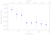 |
Fig. 13 Image of the primary (left panel) and secondary components (right panel) reconstructed from the relative flux contributions. The black line represents an ellipse with ellipticity of 0.6 and 0.7 for the primary and secondary components, respectively. |
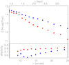 |
Fig. 14 Surface brightness (upper panel) and ellipticity (lower panel) radial profile of the primary (blue) and secondary (red) stellar components. |
4.5 Star formation rate
The current SFR spatial distribution can show possible links between the ionized gas and the stellar counter-rotating disk. In addition, the present-day SFR activity can provide clues about the epoch of gas acquisition when considering scenarios in which the counter-rotating disk formed in situ from acquired gas. Finally, the SFR intensity allows a comparison of IC 719 with normal (co-rotating) galaxies.
To derive the SFR in IC 719, we first identified the galaxy’s star-forming region adopting the standard emission lines diagrams from Baldwin et al. (1981, BPT diagrams hereafter) as applied by Kauffmann et al. (2003) and Kewley et al. (2001) (Fig.17). According to the BPT diagnostics, the regions dominated by star formation describe a large elliptical annulus with an inner semi-major axis of 5′′. We can trace star formation activity up to the last measured point at about 30′′. Instead, the inner bulge regions are dominated by shocks (Fig. 19). The highest star formation activity is located in a thin elliptical ring within ~7 and ~ 12′′, with the same geometry and size as the K-band ring observed by Katkov et al. (2013).
The SFR map was estimated considering the H α emission and Eq. (2)of Kennicutt (1998) adopting the extinction map obtained from the H β and H α ratio following Catalán-Torrecilla et al. (2015) (Fig. 18). In Fig. 19 we plot the resulting SFR map.
The total SFR of IC 719 is ~0.5 M⊙ y−1, that is, an intermediate value between the star forming galaxies and “retired” galaxies (Cano-Díaz et al. 2016).
The SFR surface density radial profile was derived in the same way as the radial profiles of age and metallicity, and plotted in Fig. 20. The maximum of the SFR is in the star-forming ring; it has a value of 32 ± 8 M⊙ Gyr−1 pc−2 at r = 10′′ and then decreases with a slope of about 0.7M⊙ Gyr−1 pc−2∕HLR (where HLR is the half-light-radius that for IC 719 is ~ 1.9 kpc). These values and trend are consistent with the values of a typical spiral galaxy (Catalán-Torrecilla et al. 2015).
5 Discussion and conclusion
We have analyzed the integral field data with a spectral decomposition technique in order to separate and independently analyze the properties of the two stellar components in the S0 galaxy IC 719.
Our analysis confirms the main results by Katkov et al. (2013): IC 719 has two extended stellar components that rotate along opposite directions. The ionized-gas co-rotates with the secondary stellar component, which is the younger, less luminous, and less massive. In addition, the analysis of the emission lines reveals that star formation isstill active in IC 719 and it is the main source of ionization of the gas. All these elements strongly highlight the link between the secondary stellar component and the ionized-gas disk, supporting the idea that the secondary stellar component has been generated by the acquired gas disk, itself associated to a galaxy, in the case of a gas-richminor merger, or not. In this latter case, we are not detecting the pre-merger stars of the dwarf galaxy.
Thanks to the larger field of view of our MUSE data and the better spectral resolution in the CaT wavelength region used to derive the kinematics of the various components in IC 719, we are able to add some important elements with respect the previous studies on this galaxy.
First, we measure a clear difference in the stellar velocity dispersion of the two stellar components. Specifically, the main component has larger velocity dispersion whereas the secondary component has smaller velocity dispersion.
Second, our data allow us to study the 2D morphology of the stellar components, and therefore we have a complete description of their surface brightness profiles and geometry. The main component has an exponential profile with scale radius rH ~ 1.5 kpc and an observed axial ratio in the range q = 0.40−0.30. The secondary component has an exponential profile with scale rH ~ 1.0 kpc and is thinner than the main component, having an observed axial ratio in the range q = 0.25−0.20. This axial ratio is compatible with that of a very thin disk observed at an inclination of i = 77°. In fact, if we use the value of i = 77° to deproject the two disks, we find that the main component has an intrinsic axial ratio of 0.2–0.3 while the secondary component has an axial ratio ≤0.15. While the main component has an intrinsic thickness comparable with a typical disk galaxy (Rodríguez & Padilla 2013), the secondary component has an intrinsic thickness similar to that of a very thin disk, as we expect for ionized gas.
The results on the stellar velocity dispersion and flattening put some important constraints on the formation scenario and strengthen previous conclusions. In the binary galaxy merger scenario (Crocker et al. 2009), the ionized gas component is expected to co-rotate with the thicker, dynamically hotter, and more massive component. This is true for a perfectly co-planar geometry of the encounter. Qu et al. (2011) studied the case of 1:10 minor mergers with different geometries. In general, they find that the acquired counter-rotating stars form a counter-rotating thick stellar disk. Our measurements of the velocity dispersion and flattening indicate the opposite and are therefore consistent with the scenario in which the counter-rotating stars formed from gas acquired from either a gas cloud or a gas-rich dwarf galaxy.
Star formation and gas accretion are still ongoing in IC 719. In fact, as pointed out by Katkov et al. (2013), the galaxy is surrounded by a considerable amount of HI (Grossi et al. 2009) that is probably the source of the ionized gas. It seems to form a commonenvelope with the HI surrounding the companion IC 718 which is located at a projected distance of 96 kpc.
In their work, Katkov et al. (2013) advocate the scenario in which the external gas was accreted by IC 719 in two distinct episodes, both followed by star formation, in contrast with the alternative scenario of a single accretion episode followed by two bursts of star formation. In this picture, the HI is likely still in the process of falling onto the galaxy. The main argument in favor of two accretion events is that the metallicity of the ionized gas is lower than the metallicity of the secondary stellar component; it would be the opposite if the generation of stars were formed by a second burst using gas processed by the first generation of stars. In this picture, the different radial behavior of the metallicity of the gas-phase with respect to the secondary stellar component may indicate that the gas experienced, after the star formation, prolonged or continuous gas acquisition (like in NGC 5719) and/or enrichment caused by the stellar evolution.
The age gradient we measure is consistent with the scenario proposed by Katkov et al. (2013). The accretion and star formation occurred ~4 Gyr ago and created the first generation of stars in the secondary component. The second accretion and burst dominated the inner ~ 2.5 kpc, where younger luminosity-weighted ages are measured and the star formation activity is higher. The fact that the stellar metallicity is higher than that of the gas phase in the inner ~2 kpc is also consistent with this picture: the stars in the central region originated from the accreted gas and gas that has been re-processed and enriched by the previous generation of stars, resulting in a higher metallicity. The flat radial profile of the gas-phase metallicity supports the idea that the two accreted gas masses come from the same source, most likely the HI cloud surrounding IC 719.
It is interesting to study how IC 719 compares with other galaxies that host counter-rotating stellar components. We found a similar system in NGC 5719 where an HI bridge is connecting it to NGC 5718. NGC 5719 hosts a counter-rotating disk younger than the main galaxy and with a ring of star formation of about 1 kpc radius. A third galaxy that shows similar behavior is NGC 3595. Here the star-forming ring has a diameter of about 1 kpc. Grossi et al. (2009) find this galaxy to be an early-type galaxy given the great amount of HI contained within. Bettoni et al. (2014) considered this latter object as a case of rejuvenation induced by the acquisition of gas. In this respect, it would be interesting to know how IC 719 would look like if the gas was acquired in pro-grade orbits. Most likely it would appear like a normal Sb galaxy or possibly host a star-forming nuclear ring (see Ma et al. 2017, and references therein). For instance, Mapelli et al. (2015) studied the formation of gas rings in an S0 galaxy as a consequence of a gas-rich minor merger for both prograde and retrograde encounters. They found, by means of N-body/smoothed particle hydrodynamics simulations, that in both cases a warm gas ring forms and causes a rejuvenation of the stellar population. For NGC 448, Katkov et al. (2016) suggested a different formation mechanism. In this case, they exclude a cosmic gas filament as the origin of the acquired gas. They preferred a satellite merger with slow gas accretion as the origin of the counter-rotating stellar disk. On the other hand, NGC 448 shows no star formation activity and an old stellar population (9 Gyr) for both components and can be seen as the evolution of systems like IC 719. This is probably true for other counter-rotating systems such as NGC 4550 and NGC 4191 that show a small amount of gas, no ongoing star formation, and a relatively old stellar population in the acquired component.
In summary, IC 719 represents a clear case of an S0 galaxy hosting two stellar counter-rotating disks. Thanks to the large field of viewand wavelength coverage of the MUSE spectrograph, we are able to add further constraints to the formation mechanisms. In particular, we can unveil the structural and kinematical differences between the two stellar components. We confirm the previous scenario in which the secondary stellar component of IC 719 formed via multiple accretion of gas coming from the surrounding HI cloud followed by star formation episodes.
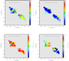 |
Fig. 15 Upper panels: stellar population age for the primary (left panel) and secondary (right panel) components. Lower panels: stellar population metallicity for the primary (left panel) and secondary (right panel) components. |
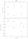 |
Fig. 16 Age (upper panel) and metallicity (lower panel) as a function of radius along the major axis of IC 719. Blue points represent the primary component and red points the secondary component. In the lower panel, open squares mark the gas-phase metallicity measured by means of the [N II] λ6583 (green) and [N II] λ6583 + [O III] λ5007 (light green) emission lines. |
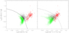 |
Fig. 17 BPT diagram on the [N II] λ6583, [O III] λ5007, H β and H α lines. Red dots indicate the measurements belonging to the inner 3′′ deprojectedradius. The black full and dashed lines delimit the star-forming regions as indicated by Kauffmann et al. (2003) and Kewley et al. (2001). In both panels, green dots are the points that fall in the SFR region following both criteria. |
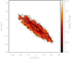 |
Fig. 18 Extinction map A(Hα) derived following Catalán-Torrecilla et al. (2015). |
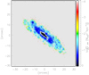 |
Fig. 19 Color-coded SFR surface density map of IC 719. Black dots indicate the region where the BPT diagnostic indicates emission dominated by shocks. The gray region indicates where the signal was too low. |
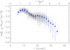 |
Fig. 20 Surface SFR as a function of the deprojected radius. Dots indicate measurements in each spaxel. Blue dots and error-bars are the mean and the RMS computed in different radial bins. SFR has been deprojected for inclination. |
Acknowledgements
This work was supported by Padua University through grants 60A02-5857/13, 60A02-5833/14, 60A02-4434/15, and CPDA133894. AP and LC thank the European Southern Observatory and Department of Physics and Astronomy of the University of Padova, respectively, for hospitality during the development of this paper. LM and EMC acknowledge financial support from Padua University grants CPS0204 and BIRD164402/16, respectively.
References
- Algorry, D. G., Navarro, J. F., Abadi, M. G., et al. 2014, MNRAS, 437, 3596 [NASA ADS] [CrossRef] [Google Scholar]
- Bacon, R., Accardo, M., Adjali, L., et al. 2010, in Ground-based and Airborne Instrumentation for Astronomy III, Proc. SPIE, 7735, 773508 [Google Scholar]
- Baldwin, J. A., Phillips, M. M., & Terlevich, R. 1981, PASP, 93, 5 [NASA ADS] [CrossRef] [EDP Sciences] [Google Scholar]
- Bassett, R., Bekki, K., Cortese, L., & Couch, W. 2017, MNRAS, 471, 1892 [NASA ADS] [CrossRef] [Google Scholar]
- Beifiori, A., Maraston, C., Thomas, D., & Johansson, J. 2011, A&A, 531, A109 [NASA ADS] [CrossRef] [EDP Sciences] [Google Scholar]
- Bertola, F., & Corsini, E. M. 1999, in Galaxy Interactions at Low and High Redshift, eds. J. E. Barnes & D. B. Sanders, IAU Symp., 186, 149 [NASA ADS] [CrossRef] [Google Scholar]
- Bertola, F., Cinzano, P., Corsini, E. M., et al. 1996, ApJ, 458, L67 [NASA ADS] [CrossRef] [Google Scholar]
- Bertola, F., Corsini, E. M., Vega Beltrán, J. C., et al. 1999, ApJ, 519, L127 [NASA ADS] [CrossRef] [Google Scholar]
- Bettoni, D., Mazzei, P., Rampazzo, R., et al. 2014, Ap&SS, 354, 83 [NASA ADS] [CrossRef] [Google Scholar]
- Cano-Díaz, M., Sánchez, S. F., Zibetti, S., et al. 2016, ApJ, 821, L26 [NASA ADS] [CrossRef] [Google Scholar]
- Cappellari, M., & Copin, Y. 2003, MNRAS, 342, 345 [NASA ADS] [CrossRef] [Google Scholar]
- Cappellari, M., & Emsellem, E. 2004, PASP, 116, 138 [NASA ADS] [CrossRef] [Google Scholar]
- Catalán-Torrecilla, C., Gil de Paz, A., Castillo-Morales, A., et al. 2015, A&A, 584, A87 [NASA ADS] [CrossRef] [EDP Sciences] [Google Scholar]
- Chung, A., Bureau, M., van Gorkom, J. H., & Koribalski, B. 2012, MNRAS, 422, 1083 [NASA ADS] [CrossRef] [Google Scholar]
- Ciri, R., Bettoni, D., & Galletta, G. 1995, Nature, 375, 661 [NASA ADS] [CrossRef] [Google Scholar]
- Coccato, L., Morelli, L., Corsini, E. M., et al. 2011, MNRAS, 412, L113 [NASA ADS] [CrossRef] [Google Scholar]
- Coccato, L., Morelli, L., Pizzella, A., et al. 2013, A&A, 549, A3 [NASA ADS] [CrossRef] [EDP Sciences] [Google Scholar]
- Coccato, L., Iodice, E., & Arnaboldi, M. 2014, A&A, 569, A83 [NASA ADS] [CrossRef] [EDP Sciences] [Google Scholar]
- Coccato, L., Fabricius, M., Morelli, L., et al. 2015, A&A, 581, A65 [NASA ADS] [CrossRef] [EDP Sciences] [Google Scholar]
- Corsini, E. M. 2014, in Multi-Spin Galaxies, eds. E. Iodice, & E. M. Corsini, ASP Conf. Ser., 486, 51 [NASA ADS] [Google Scholar]
- Corsini, E. M., Pizzella, A., & Bertola, F. 2002, A&A, 382, 488 [NASA ADS] [CrossRef] [EDP Sciences] [Google Scholar]
- Corsini, E. M., Méndez-Abreu, J., Pastorello, N., et al. 2012, MNRAS, 423, L79 [NASA ADS] [CrossRef] [Google Scholar]
- Crocker, A. F., Jeong, H., Komugi, S., et al. 2009, MNRAS, 393, 1255 [NASA ADS] [CrossRef] [Google Scholar]
- de Vaucouleurs, G., de Vaucouleurs, A., Corwin, Jr. H. G., et al. 1991, Third Reference Catalogue of Bright Galaxies (New York: Springer) [Google Scholar]
- Evans, N. W.,& Collett, J. L. 1994, ApJ, 420, L67 [NASA ADS] [CrossRef] [Google Scholar]
- Fabricius, M. H., Coccato, L., Bender, R., et al. 2014, MNRAS, 441, 2212 [NASA ADS] [CrossRef] [Google Scholar]
- Falcón-Barroso, J., Sánchez-Blázquez, P., Vazdekis, A., et al. 2011, A&A, 532, A95 [NASA ADS] [CrossRef] [EDP Sciences] [Google Scholar]
- Freudling, W., Romaniello, M., Bramich, D. M., et al. 2013, A&A, 559, A96 [NASA ADS] [CrossRef] [EDP Sciences] [Google Scholar]
- Galletta, G. 1996, in IAU Colloq. 157: Barred Galaxies, eds. R. Buta, D. A. Crocker, & B. G. Elmegreen, ASP Conf. Ser., 91, 429 [NASA ADS] [Google Scholar]
- Gerssen, J., & Shapiro Griffin K. 2012, MNRAS, 423, 2726 [NASA ADS] [CrossRef] [Google Scholar]
- Grossi, M., di Serego Alighieri, S., Giovanardi, C., et al. 2009, A&A, 498, 407 [NASA ADS] [CrossRef] [EDP Sciences] [Google Scholar]
- Johnston, E. J., Merrifield, M. R., Aragón-Salamanca, A., & Cappellari, M. 2013, MNRAS, 428, 1296 [NASA ADS] [CrossRef] [Google Scholar]
- Katkov, I., Chilingarian, I., Sil’chenko, O., Zasov, A., & Afanasiev, V. 2011, Baltic Astronomy, 20, 453 [NASA ADS] [Google Scholar]
- Katkov, I. Y., Sil’chenko, O. K., & Afanasiev, V. L. 2013, ApJ, 769, 105 [NASA ADS] [CrossRef] [Google Scholar]
- Katkov, I. Y., Sil’chenko, O. K., Chilingarian, I. V., Uklein, R. I., & Egorov, O. V. 2016, MNRAS, 461, 2068 [NASA ADS] [CrossRef] [Google Scholar]
- Kauffmann, G., Heckman, T. M., White, S. D. M., et al. 2003, MNRAS, 341, 54 [Google Scholar]
- Kennicutt, Jr. R. C. 1998, ARA&A, 36, 189 [Google Scholar]
- Kewley, L. J., Dopita, M. A., Sutherland, R. S., Heisler, C. A., & Trevena, J. 2001, ApJ, 556, 121 [Google Scholar]
- Ma, C., de Grijs, R., & Ho, L. C. 2017, ApJS, 230, 14 [NASA ADS] [CrossRef] [Google Scholar]
- Mapelli, M., Rampazzo, R., & Marino, A. 2015, A&A, 575, A16 [NASA ADS] [CrossRef] [EDP Sciences] [Google Scholar]
- Marino, R. A., Rosales-Ortega, F. F., Sánchez, S. F., et al. 2013, A&A, 559, A114 [NASA ADS] [CrossRef] [EDP Sciences] [Google Scholar]
- Mehlert, D., Thomas, D., Saglia, R. P., Bender, R., & Wegner, G. 2003, A&A, 407, 423 [NASA ADS] [CrossRef] [EDP Sciences] [Google Scholar]
- Mitzkus, M., Cappellari, M., & Walcher, C. J. 2017, MNRAS, 464, 4789 [Google Scholar]
- Morelli, L., Corsini, E. M., Pizzella, A., et al. 2012, MNRAS, 423, 962 [NASA ADS] [CrossRef] [Google Scholar]
- Morelli, L., Parmiggiani, M., Corsini, E. M., et al. 2016, MNRAS, 463, 4396 [NASA ADS] [CrossRef] [Google Scholar]
- Morelli, L., Pizzella, A., Coccato, L., et al. 2017, A&A, 600, A76 [NASA ADS] [CrossRef] [EDP Sciences] [Google Scholar]
- Munari, U., Sordo, R., Castelli, F., & Zwitter, T. 2005, A&A, 442, 1127 [NASA ADS] [CrossRef] [EDP Sciences] [Google Scholar]
- Osterbrock, D. E., Fulbright, J. P., Martel, A. R., et al. 1996, PASP, 108, 277 [NASA ADS] [CrossRef] [Google Scholar]
- Osterbrock, D. E., Fulbright, J. P., & Bida, T. A. 1997, PASP, 109, 614 [NASA ADS] [CrossRef] [Google Scholar]
- Pizzella, A., Morelli, L., Corsini, E. M., et al. 2014, A&A, 570, A79 [NASA ADS] [CrossRef] [EDP Sciences] [Google Scholar]
- Puerari, I., & Pfenniger, D. 2001, Ap&SS, 276, 909 [Google Scholar]
- Qu, Y., Di Matteo, P., Lehnert, M. D., van Driel, W., & Jog, C. J. 2011, A&A, 535, A5 [NASA ADS] [CrossRef] [EDP Sciences] [Google Scholar]
- Rodríguez, S., & Padilla, N. D. 2013, MNRAS, 434, 2153 [NASA ADS] [CrossRef] [Google Scholar]
- Rubin, V. C., Graham, J. A., & Kenney, J. D. P. 1992, ApJ, 394, L9 [NASA ADS] [CrossRef] [Google Scholar]
- Sarzi, M., Corsini, E. M., Pizzella, A., et al. 2000, A&A, 360, 439 [NASA ADS] [Google Scholar]
- Sarzi, M., Bertola, F., Cappellari, M., et al. 2001, Ap&SS, 276, 467 [NASA ADS] [CrossRef] [Google Scholar]
- Sommariva, V., Mannucci, F., Cresci, G., et al. 2012, A&A, 539, A136 [NASA ADS] [CrossRef] [EDP Sciences] [Google Scholar]
- Tabor, M., Merrifield, M., Aragón-Salamanca, A., et al. 2017, MNRAS, 466, 2024 [NASA ADS] [CrossRef] [Google Scholar]
- Thakar, A. R., & Ryden, B. S. 1998, ApJ, 506, 93 [NASA ADS] [CrossRef] [Google Scholar]
- Thakar, A. R., Ryden, B. S., Jore, K. P., & Broeils, A. H. 1997, ApJ, 479, 702 [NASA ADS] [CrossRef] [Google Scholar]
- Thomas, D., & Maraston, C. 2003, A&A, 401, 429 [NASA ADS] [CrossRef] [EDP Sciences] [Google Scholar]
- Thomas, D., Maraston, C., & Johansson, J. 2011, MNRAS, 412, 2183 [NASA ADS] [CrossRef] [Google Scholar]
- Vazdekis, A., Ricciardelli, E., Cenarro, A. J., et al. 2012, MNRAS, 424, 157 [NASA ADS] [CrossRef] [Google Scholar]
- Weilbacher, P. M., Streicher, O., Urrutia, T., et al. 2012, in Software and Cyberinfrastructure for Astronomy II, Proc. SPIE, 8451, 84510B [NASA ADS] [CrossRef] [Google Scholar]
IRAF is the Image Reduction and Analysis Facility, written and supported by the National Optical Astronomy Observatories (NOAO).
12 + log(O/H) = 8.743 + 0.462 × log([N II]∕Hα), and 12 + log(O/H) = 8.533 − 0.214 × log(([O III]∕Hβ)∕(Ha∕[N II])).
log(Z∕Z⊙) = 12 + log(O∕H) − 8.69.
All Figures
|
Fig. 1 MUSE image of IC 719. The image was obtained by averaging the wavelength range 7500–8000 Å. The image intensity is shown with a logarithmic scale. The field of view and orientation of all 2D maps of the paper are ~ 1′ × 1′ and north up, east left. |
| In the text | |
|
Fig. 2 Example of the observed (black line) and fitted spectrum in a bin where the two stellar components appear separated. Here the fit is limited to the CaT wavelength region. We show the two stellar spectra fitted to the data (blue and red lines), and their sum (magenta line). The green line represents the residuals shifted upward by 1.5 units. The yellow regions are regions masked and not included in the fit. |
| In the text | |
|
Fig. 3 As in Fig. 2 but considering the whole wavelength extension. The cyan line represents the ionized gas emissionwhile the magenta line represents the sum of the two stellar components and the ionized gas emission. |
| In the text | |
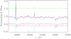 |
Fig. 4 Zoom in on the Hβ and Mg spectralregion of Fig. 3. |
| In the text | |
|
Fig. 5 Velocity field of the main component (left panel), secondary component (center panel), and of the ionized gas component (right panel). Typical errors are 7 km s−1 for the stellar components and 2 km s−1 for the ionized gas. |
| In the text | |
|
Fig. 6 As in Fig. 5 for the velocity dispersion field. Typical errors are 10 km s−1 for the stellar components and 2 km s−1 for the ionized gas. |
| In the text | |
|
Fig. 7 Velocity (left panel) and velocity dispersion curve (right panel) extracted along the major axis of IC 719. Blue, red, and green lines represent the main stellar component, secondary stellar component, and ionized gas, respectively. The velocity of the main component has been changed in sign in order to allow a direct comparison with the velocity of the other two components. The instrumental velocity dispersion of 35 km s−1 (CaT) and 53 km s−1 (Hα ) is indicated as reference by a horizontal tick. The extraction of the kinematics along the major axis has been doneby spatial averaging the spaxels in Figs. 5 and 6 considering a 2′′ -wide aperture passing thought the center along PA = 53°. Typical error-bars on the velocity and velocity dispersion are 5 and 10 km s−1, respectively. |
| In the text | |
|
Fig. 8 Emission line maps, from top left to bottom right panel, for Hβ, H α, [N II] λ6583, and [S II] λ6716. The field of view is 1′× 1′. N is up and E is left. |
| In the text | |
|
Fig. 9 Equivalent width map of the main component for the Hβ, Mgb, Fe5270, and Fe5335 absorption lines. The color indicates the EW in each bin as indicated by the color bar. The field of view is 1′ × 1′. N is up and E is left. |
| In the text | |
 |
Fig. 10 As in Fig. 9 but for the secondary component. |
| In the text | |
|
Fig. 11 Lick indices for the main component (left panel, blue dots) and the secondary component (right panel, red dots). The color tonality indicates the position of the measurement with lighter colors for the central regions and darker colors for the external regions. The lines are the loci of constant age and metallicity as indicates by the labels. |
| In the text | |
|
Fig. 12 Luminosity fraction of the secondary component over the total, as a function of radius. |
| In the text | |
|
Fig. 13 Image of the primary (left panel) and secondary components (right panel) reconstructed from the relative flux contributions. The black line represents an ellipse with ellipticity of 0.6 and 0.7 for the primary and secondary components, respectively. |
| In the text | |
|
Fig. 14 Surface brightness (upper panel) and ellipticity (lower panel) radial profile of the primary (blue) and secondary (red) stellar components. |
| In the text | |
|
Fig. 15 Upper panels: stellar population age for the primary (left panel) and secondary (right panel) components. Lower panels: stellar population metallicity for the primary (left panel) and secondary (right panel) components. |
| In the text | |
|
Fig. 16 Age (upper panel) and metallicity (lower panel) as a function of radius along the major axis of IC 719. Blue points represent the primary component and red points the secondary component. In the lower panel, open squares mark the gas-phase metallicity measured by means of the [N II] λ6583 (green) and [N II] λ6583 + [O III] λ5007 (light green) emission lines. |
| In the text | |
|
Fig. 17 BPT diagram on the [N II] λ6583, [O III] λ5007, H β and H α lines. Red dots indicate the measurements belonging to the inner 3′′ deprojectedradius. The black full and dashed lines delimit the star-forming regions as indicated by Kauffmann et al. (2003) and Kewley et al. (2001). In both panels, green dots are the points that fall in the SFR region following both criteria. |
| In the text | |
|
Fig. 18 Extinction map A(Hα) derived following Catalán-Torrecilla et al. (2015). |
| In the text | |
|
Fig. 19 Color-coded SFR surface density map of IC 719. Black dots indicate the region where the BPT diagnostic indicates emission dominated by shocks. The gray region indicates where the signal was too low. |
| In the text | |
|
Fig. 20 Surface SFR as a function of the deprojected radius. Dots indicate measurements in each spaxel. Blue dots and error-bars are the mean and the RMS computed in different radial bins. SFR has been deprojected for inclination. |
| In the text | |
Current usage metrics show cumulative count of Article Views (full-text article views including HTML views, PDF and ePub downloads, according to the available data) and Abstracts Views on Vision4Press platform.
Data correspond to usage on the plateform after 2015. The current usage metrics is available 48-96 hours after online publication and is updated daily on week days.
Initial download of the metrics may take a while.