| Issue |
A&A
Volume 615, July 2018
|
|
|---|---|---|
| Article Number | A55 | |
| Number of page(s) | 12 | |
| Section | Extragalactic astronomy | |
| DOI | https://doi.org/10.1051/0004-6361/201732275 | |
| Published online | 12 July 2018 | |
Stellar populations of HII galaxies
A tale of three bursts
1
Observatório Nacional, Rua José Cristino,
77,
Rio de Janeiro
20921-400,
Brazil
e-mail: etelles@on.br
2
European Southern Observatory,
Av. Alonso de Córdova 3107,
Santiago,
Chile
Received:
10
November
2017
Accepted:
4
March
2018
Aims. We present a UV to mid-IR spectral energy distribution (SED) study of a large sample of SDSS DR13 HII galaxies. These galaxies are selected as starbursts (EW(Hα) > 50Å) and for their high-excitation locus in the upper left region of the BPT diagram. Their photometry was derived from the cross-matched GALEX, SDSS, UKDISS, and WISE catalogs.
Methods. We used CIGALE modeling and a SED fitting routine with the parametrization of a three-burst star formation history, and a comprehensive analysis of all other model parameters. We were able to estimate the contribution of the underlying old stellar population to the observed equivalent width of Hβ, and allow for more accurate burst age determination.
Results. We found that the star formation histories of HII Galaxies can be reproduced remarkably well by three major eras of star formation. In addition, the SED fitting results indicate that in all cases the current burst produces a small percent of the total stellar mass, i.e., the bulk of stellar mass in HII galaxies has been produced by the past episodes of star formation, and also indicate that at a given age the Hβ luminosity depends only on the mass of young stars favoring a universal IMF for massive stars. Most importantly, the current star formation episodes are maximum starbursts that produce stars at the highest possible rate.
Key words: galaxies: dwarf / galaxies: starburst / galaxies: stellar content / galaxies: star formation
© ESO 2018
1 Introduction
HII Galaxies are compact dwarf starburst galaxies with strong, narrow emission lines superposed on a weak, blue continuum. The optical spectra of HII Galaxies are indistinguishable from those of Giant HII regions in local galaxies (Sargent & Searle 1970). It is now widely accepted that they are not bona fide young galaxies forming their first generation of stars, as was thought in the past, since they all show a population of old stars.
Westera et al. (2004) used the spectra of approximately 100 HII galaxies to assess their stellar population content and history by deriving absorption line indexes (based on Hδ, H+K(Ca), Mgb, and D4000) and compared these spectra with stellar population models of SB99 (Leitherer et al. 1999) and BC03 (Bruzual & Charlot 2003). The main conclusion from that work is that, mostly, we can parametrize the star formation history (SFH) of HII galaxies with these three main stellar populations.
Optical (Telles et al. 1997; Telles & Terlevich 1997) and near-IR imaging (Lagos et al. 2011, and references therein) have also convincingly shown that these dwarf starburst galaxies possess underlying old populations. Simulations also show the episodic nature of star-forming galaxies, particularly at low masses (see, e.g., Pelupessy et al. 2004; Debsarma et al. 2016), thus making three episodes the simplest choice in this scenario.
The morphologies of HII galaxies remain as first described, a “mixed bag” (Loose & Thuan 1986; Kunth et al. 1988). The general properties of HII galaxies and blue compact galaxies (BCG) broadly overlap (Kunth & Östlin 2000). They have irregular shapes, typically small physical sizes, and no signs of ordered structures such as disks. Their starburst regions, consisting of emsembles of massive ionizing clusters and their respective giant HII regions cover most of the extension of their optical images. More luminous HII galaxies seem to show some evidence of tails, fuzz in their outermost isophotes, and more disturbed overall morphologies, whereas the lower luminosity galaxies seem more compact (Telles et al. 1997). Deeper optical imaging (Lagos et al. 2007) and near-IR imaging (Lagos et al. 2011) reveal the clumpy nature of their starburst regions. The various subclassification attempts, such as cometary (Papaderos et al. 2008), local tadpoles (Elmegreen et al. 2012), green-peas (Cardamone et al. 2009), all fall within the mixed bag of clumpy morphology with no fundamental differences in their intrinsic properties. Due to their low mass, low oxygen abundance, low dust content, and low-density environments, HII galaxies constitute the simplest starbursts at galactic scales.
With the advent of large surveys, particularly the Sloan Digital Sky Survey (SDSS; York et al. 2000), star-forming galaxies all fall into a uniform spectroscopic class and are viewed in a more general common perspective. Total stellar mass seems to be the main driver of the properties of the star-forming galaxies at low redshift (Brinchmann et al. 2004; Tremonti et al. 2004). However, the locus where emission line galaxies fall in the BPT diagram (Baldwin et al. 1981) determines some important general properties as well since the star-forming sequence is also a sequence of increasing excitation with the decrease in stellar mass and metallicity (Curti et al. 2017, and references therein).
HII Galaxies are particularly interesting as cosmological probes over a surprisingly wide range of redshifts that extend to redshifts of z = 3−4 with present-day instrumentation. Their emission line luminosities, in particular the Balmer lines, correlate extremely well with the velocity-widths of the same emission lines (Terlevich & Melnick 1981; Melnick et al. 1988; Telles & Terlevich 1993; Bordalo et al. 2009; Bordalo & Telles 2011; Chávez et al. 2014). This is known as the L-σ relation, and it can be calibrated as a distance indicator using Giant HII regions in local galaxies, and can thus be used to determine cosmological parameters (Melnick et al. 2000; Plionis et al. 2011; Terlevich et al. 2015; Chávez et al. 2016; Fernández-Arenas et al. 2018). Since the L-σ method is independent from other methods, a cross comparison of results can help us better understand the systematic uncertainties in these different methods, most notably the SNIa.
While it seems clear that the L-σ relation stems from the natural relation between the ionizing flux of a starburst and the mass of its ionizing cluster, the relation is empirical and thus suffers from considerable intrinsic scatter. In Melnick et al. (2017) we explored ways of reducing the scatter, but stumbled against the difficulty of accurately measuring the ages of the young components. The traditional age indicator, the equivalent width of Hβ (EW(Hβ)), is biased by contamination of the continuum by older underlying populations, and therefore age corrections using EW(Hβ) tend to increase the scatter rather than reduce it.
In this paper we make use of multiwavelength stellar population analysis by using the method of fitting the spectral energy distribution (SED) from the UVto the mid-IR (MIR) in order to describe the simplest star formation history for HII galaxies that accommodates their general properties. We want to investigate how efficiently HII galaxies form stars in their present bursts compared to their past histories. We also retrieve the true distribution of EW(Hβ) for the young stellar component of our sample by applying a correction factor fr that accounts for the contamination of the continuum by the old stellar population derived from our stellar population analysis. This will help us further understand, and possibly reduce, the systematic errors related to the use of the L-σ as a powerful indicator of cosmological distances. Section 2 presents our data selection of extreme star-forminggalaxies from the Sloan Digital Sky Survey. Section 3 describes our SED fitting model, model choices, and procedure. In Sect. 4 we present our results, and conclusions are given in Sect. 5.
2 Data and general spectral properties
Our data are selected from the SDSS DR13 release (Albareti et al. 2017) cross-matched with the emissionLinePort table,1 and contains galaxies classified as subclass STARBURST which implies EW (Hα) > 50Å. These criteria reflect in over 67 000 galaxies. From these galaxies we selected only those with EW (Hβ) > 30Å and those whoseline ratios fall within the upper left panel of the canonical interval for star-forming regions in the BPT diagram (Baldwin et al. 1981; Kewley et al. 2006). These choices were made in order to select extreme star-forming galaxies with high excitation, low abundances, and low masses, characteristics typical of bona fideHII galaxies. So, our selection criteria are more restrictive and do not include more luminous star-forminggalaxies. These criteria allow the inclusion of the lowest metallicity objects which have slightly lower [OIII]/Hβ ratios due to their low ionic abundances (Izotov et al. 2018). In order to avoid including local giant HII regions in nearby galaxies, we also restricted the sample to z > 0.005, resulting in ~4200 SDSS objects. Figure 1 shows the selected spectroscopic sample. A summary of these criteria is given in Table 1.
For our final sample of HII galaxies for our multiwavelength analysis from far-UV (FUV) to MIR, we chose from the SDSS sample only targets with GALEX unique photometry in both FUV (0.1528 μm) and near-UV (NUV; 0.2271 μm) bands (Bianchi 2014, and references therein). The resulting GALEX+SDSS sample of HII galaxies consists of 2728 objects. For this sample we cross-matched targets with the UKIRT Infrared Deep Sky Survey (Lawrence et al. 2007, UKIDSS) Y (1.036 μm), J (1.250 μm), H (1.644 μm), and K (2.149,μm) near-IR (NIR) bands, and with the Wide-Field Infrared Survey Explorer (WISE; Wright et al. 2010) W1 (3.4 μm), W2 (4.6 μm), W3 (12 μm), W4 (22 μm) MIRbands.
In the end, we chose not to use the W3 and W4 bands since we are more concerned with the stellar population properties as a result of our analysis, and these bands only undergo a significant effect at these longer wavelengths due to the dust emission component. Table 2 shows the resulting photometric sample of HII galaxies. The most restrictive photometric band is the UKIDSS with NIR data for only one-third of our sample. In our analysis we used all the available photometric data for each individual galaxy. To minimize systematic effects we used Petrosian magnitudes except for GALEX for which we used model magnitudes. Our choice of the Petrosian magnitudes ensures that in all bands we measured the fluxes in the same way to include the same percentage of the total flux. Our objects are compact (see Fig. 2), thus aperture effects are minimized since we are probably including all the flux in all bands. We also correlated with VISTA surveys, but found no additional targets.
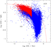 |
Fig. 1 BPT diagram of the selected objects. The blue points are the whole sample of 67 000 starburst galaxies. The red points are the resulting spectroscopic sample of ~4200 galaxies with the criteria given in Table 1. HII galaxies lie below and to the left of the Kauffmann et al. (2003) classification (solid red line) that distinguishes AGNs from star-forming galaxies. |
Summary of the selection criteria of our spectroscopic sample, resulting in our SDSS sample of ~4200 objects.
Number of objects that have the corresponding photometric data from the given surveys.
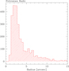 |
Fig. 2 Distribution of the Petrosian radius in the SDSS r band of our photometric sample of 2728 HII galaxies. The median value of the distribution is only 2.8′′. |
2.1 Basic properties
Figure 3 shows the spectroscopic characterization of our cross-matched GALEX+SDSS sample of 2728 HII galaxies. The figure shows histograms of the logarithmic extinction correction factor C(Hβ), the observed equivalent width of Hβ, the derived Hβ luminosity,2 and the derived oxygen abundance, respectively (see below). A typical galaxy in our sample has low extinction (E(B-V) ~ 0.1), intense emission lines (EW(Hβ) ~ 50 Å, log L(Hβ) ~ 40.5 ergcm2 s−1), and low metal abundance (12 + log(O/H) ~ 8.2, Z ~ 1∕3 Z⊙).
2.2 Extinction corrections
Our first step was to correct the fluxes for foreground extinction using the maps of Schlafly & Finkbeiner (2011), as reported in the SDSS data base, and the extinction law for the Galaxy from Cardelli et al. (1989). This is relevant because in these starburst galaxies the foreground extinction is substantial, and the extinction laws for the internal extinction are very different in the UV.
As the second step, the intrinsic internal reddening is then derived from the resulting Hα/Hβ ratio (corrected for Galactic extinction) for each HII galaxy, using either a Calzetti (Calzetti et al. 2000) or a Gordon (Gordon et al. 2003) extinction law. The Gordon extinction curve is that of the SMC bar, which is the steepest curve in theUV. Their comparative results seem to indicate that there is a trend for the extinction curves to be steeper in the UV for systems of lower gas-to-dust ratios. The starburst galaxies in our sample have typically sub-solar oxygen abundances implying a low dust content, and hence this ratio will be high for our sample galaxies, favoring a SMC bar-like extinction curve. This agrees with previous findings by Gordon et al. (1997), who found that the steeper UV extinction curve seems to be associated with enhanced star formation regions such as 30 Dor in LMC whose extinction curve differs from the rest of the LMC.
We then measured the line intensities for Hα, Hβ, and Hγ by optimizing the placement of the continuum and carefully adjusting the integration box to include all the line fluxes. Inspection of the spectra showed that in general the higher Balmer lines (λ ≤ Hδ4101Å) were embedded in a stellar absorption feature that appears to be significantly broader than the emission lines. For this reason we did not include these lines in our analysis. Even Hγ is in most cases somewhat affected by absorption; however, considering that the equivalent widths of the absorption features in synthetic spectra for starburst are similar for Hβ and Hγ, we did not correct the line ratios for this effect.
In Fig. 4 we plot the Balmer decrements divided by the theoretical (Case B) recombination values for Te = 11 400 K, appropriate for the mean temperature of our sample, F(Hα)/F(Hβ) = 2.855 and F(Hγ)/F(Hβ) = 0.467 (Osterbrock 1989). Thus, in this log-log plot an object with zero internal extinction would be located at (0,0), which is indicated by dashed lines. The colored solid lines in the figures show the reddening vectors for a range of 1.4 magnitudes in AV for four popular extinction laws as indicated in the captions.
For the full sample of objects (gray points) the best fitting extinction law appears to be unconstrained by our measurements. Instead, when we restrict that sample to objects with errors < 0.015 (blue crosses), the best fit appears to disfavor the law of Calzetti et al. (2000), which produces much less reddening per unit absorption (it has RV = 4.88). Therefore, we corrected our spectroscopic observations using the Balmer Decrement with a Gordon extinction law as
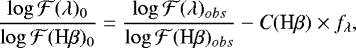 (1)
(1)
where fλ is derived from the extinction law. The resulting logarithmic extinction correction factor C(Hβ) for our sample is shown in Fig. 3.
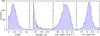 |
Fig. 3 Spectroscopic properties of our sample of intense emission line objects. From left to right panels: distribution of the Balmer decrement derived extinction parameter, distribution of the equivalent width of Hβ, distribution of Hβ luminosity, and distribution of the oxygen abundance derived from the direct method for objects with the auroral [O III]λ4363 Å line detected. This line is detected virtually in all our galaxies and allows the determination of the electron temperature (see text). |
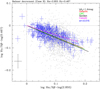 |
Fig. 4 Balmer decrements for our sample relative to the theoretical Case B recombination values for Te = 11 400 K. The solid lines represent four different extinction laws as shown for a range of Δ AV = 1.4 mag. Points in gray are for the whole sample, while points in blue correspond to objects with errors in both axes < 0.015. The black cross at the bottom left represents the mean error of the whole sample. |
2.3 Oxygen abundances
We determined the physical conditions from the emission line spectra by using the direct method, as described by the prescription of Pagel et al. (1992) and Izotov et al. (2006), since we were able to detect and measure the electron temperature sensitive emission line of [O III]λ 4363 in virtually all of our spectra (see Fig. 3, right panel). Electron densities were estimated by the ratio of the [SII] lines, [SII]λ6717/[SII]λ6731, which has a strong peak at 1.3 for our sample. This implies that all HII regions are in the low-density regime. Thus, we adopt the reasonable assumption of a constant ne of 100 cm−3.
The ionic and total abundances determined by the two prescriptions agree very well; there is a small offset of less than 0.1 towards higher abundance for the Izotov prescription, which we adopt here in order to have more recently updated atomic data. The prescription is also better suited for sub-solar abundances. While the low-abundance tail in the distribution is expected to be real and accurate, the few objects with super-solar abundance have larger uncertainties due to the lower S/N of the [OIII]λ4363 line in these cases.
3 Modeling with CIGALE
CIGALE3 (Code Investigating GALaxy Emission) is a package for SED modeling and for SED fitting. The code was developed by Denis Burgarella and Médéric Boquien at the Laboratoire d’Astrophysique de Marseille. Some applications and descriptions of CIGALE for modeling galaxy properties are found in Noll et al. (2009), Boquien et al. (2014, 2016), Ciesla et al. (2015, 2016), and Vika et al. (2017). CIGALE has a modular structure which allows great flexibility in modeling the various physical components and their possible parameters that contribute to producing the theoretical SED of galaxies. These components and the set of parameters used in our study (a subset of all possibilities) are given in Table 3. Once the predicted theoretical SED are modeled, CIGALE is used to fitting the modeled SED to the observed SED. Best fit results, probed by the output χ2, can be evaluated to provide the possible and most probable set of energy sources and their respective parameters that best represent the observed SED.
CIGALE allows for a number of star formation histories (SFH) such as exponentially declined, delayed, or periodic (see CIGALE documentation3). Our choice of the SFH consists of three episodes of star formation: a young ionizing population (< 10 Myr), an intermediate age population of (100–500 Myr), and an old stellar population (10 Gyr).
In CIGALE this particular SFH module was not implemented by default, but was developed by M. Bocquien to fit our purpose. Once we chose the SFH, we also made a choice of the evolutionary stellar population synthesis to produce our simple stellar population (SSP). We used the models of Bruzual & Charlot (2003) for a Chabrier initial mass function (IMF) and at a fixed metallicity of Z = 0.008. The choice of metallicity is justified by the fact that we have derived, from the optical spectra, their low metal content with a mean distribution of 12 + log O/H = 8.2 as shown in our Fig. 3. These are typical values for HII galaxies where the electron temperature sensitive line [OIII]λ4363 is detected (Kehrig et al. 2004; Terlevich et al. 1991). The oxygen abundances are expected to be low for our sample of high-excitation HII galaxies since they were selected to fall in the upper left locus of the star-forming sequence in the BPT diagram, which is also a metallicity sequence (see, e.g., Curti et al. 2017).
Nebular emission from the ultraviolet to the near-infrared was computed by the module Nebular that includes the emission lines and the nebular continuum. Here, for the computation of the nebular emission, we considered that the escape fraction and the absorption by dust of the Lyman continuum were both zero. We can evaluate a posteriori whether these choices were appropriate.
In all CIGALE runs we have not included a possible AGN emission component. Our targets are selected to be star-forming galaxies in the BPT diagram. It is true that AGN at low mass and low metallicity may exist and may fall in the star-forming region of the BPT (Stasińska et al. 2006), but their frequency in our sample is expected to be low, if there are any at all.
Our choice of models differs simply in the way we considered the dust attenuation and the inclusion (or not) of dust emission in order to fit the whole spectral range from the FUV to the W2 band. Table 4 shows these six runs of CIGALE. Column 1 isthe model identification, Col. 2 indicates whether or not a dust emission component was included in the runs. These are models 1, 2, and 3; the label “dl2014” indicates that the model of Dale et al. (2014) was used. The inclusion of dust emission does not affect the results significantly since dust emission becomes important only with λ > 15 μm.
The comparison between model 0 (free attenuation and no dust emission) and model 1 (free attenuation with dust emission) allows us to evaluate how much the inclusion of the dust emission interferes with the full fit. Figure 5 shows a typical example of this case. In the left panel the best fit for model 0 and in the right panel the best fit for model 1. We note that model 1 has a smaller χ2, which shows it is abetter fit to the full wavelength range including Wise bands W1 and W2. In general, the routine tries to compensate for the absence of the dust emission component in model 0 by overestimating the mass of the old stellar population. In this particular case the PAH 3.3 μm emission also contributes to the flux in the W1 band. We thus conclude that this dust emission component is necessary for any good fit in the MIR band, and contributes to a better fit in the near-infrared UKIDSS bands, as shown in this figure.
By applying analogous comparisons with the other models for which we had a choice of inclusion or not of a dust emission component, but with all other parameters being the same, such as in the case of model 2 versus model 4, and model 3 versus model 5 (see Table 4), we reach a similar conclusion, namely that models with dust emission are a better fit to the NIR data. So from this analysis we have thus favored the models where dust emission is included. Therefore, we will discard models 0, 4, and 5 for the analysis that follows.
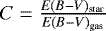
We nowhave to compare models where the attenuation corrections were left as a free parameter (model 1) to the models where the attenuation corrections were applied prior to the SED fitting procedure (model 2 versus model 3, see Col. 3 in Table 4). A choice of Gordon extinction law was used in all SED fitting runs. As mentioned above, all data were previously corrected for foreground extinction due to our Galaxy. CIGALE will output the best fitted extinction parameter C ( ), which represents the relation between the attenuation in the stellar continuum to the extinction in the nebular emission, to be either a Calzetti differential extinction (C = 0.44) or an equal extinction in the two emission components (C = 1). CIGALE uses this parameter as the ratio of the attenuation in the stellar continuum of the old stellar population to the stellar continuum of the young stellar population, not to the nebular emission. Massive young stars are embedded in the ionized HII regions, but the distribution of the young population, the older stellar population and dust may be related. However, it is not clear how these relations behave. We prefer to constrain our model to the information from the nebula emission, fixing the total amount of extinction provided by the spectral information. In addition, a comparison of the resulting χ2 for the different models reveals marginal differences. Model 2 has a distribution of χ2 marginally better than model 1. So for these two reasons we chose to keep model 2 and discard model 1.
For the remaining models (2 and 3) we pre-corrected the internal extinction using the Balmer decrement (Hα/Hβ) with the assumption of a Gordon extinction law with C = 1 (model 2)orthe Calzetti extinction law with C = 0.44 (model 3), as mentioned in Sect. 2. For these models we expect that CIGALE will simply output a residual extinction, since data were previously corrected for total extinction. The smaller this residual, the better the assumption of the attenuation law and of C.
Figure 6 shows a comparison of the output results of CIGALE for C for models 2 (green histogram) and 3 (blue histogram). This represents the residuals of attenuation that CIGALE still manages to fit and to find the best result. Model 2 has more zeros than model 3 and also more zeros than other residuals (either 0.44 or 1.0). This is not the case for model 3. This is an indication the best prior extinction correction was performed using the assumption of model 2, using a Gordon attenuation law with no differential attenuation between gas and stars (C = 1).
In summary, we chose model 2 as our best general model for the SED fitting procedure. Our results are thus derived from the SED fitting using model 2 only (see Table 4). In addition, only best fits with χ2 < 3 are considered for further analysis.
CIGALE module parameters and their ranges for SED modeling.
Models: input data set and extinction choices.
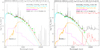 |
Fig. 5 Comparing free fit without dust emission (left panel, MODEL 0) vs. with dust emission (right panel, MODEL 1). The Green points are the observed photometry from UV to MIR. Only the first two WISE data points are shown and used inthe fits. The solid lines are the modeled components: young stellar population (cyan), intermediate+old stellar population (orange), nebular continuum (magenta), and for MODEL 1 (right panel) the dust emission (red). The red points represent the model fit results for each photometric band. The information in the inset are the respective ages and derived masses of the stellar populations. The inset also shows the observed equivalent width of Hβ (WHβ) and the corrected equivalent width of Hβ for the young stellar component only (Wy(Hβ), see text.) |
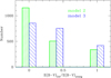 |
Fig. 6 Comparison of models 2 and 3 in relation to the residual of best fitted extinction parameter C( |
4 Results and discussion
As described in the previous section, our results are based on CIGALE model #2 (see Table 4), which includes dust emission for a better fit to the near-IR and WISE bands. The photometry has been corrected for foreground (with a Galactic extinction law) and internal extinction (with a Gordon extinction law and E(B-V)gas = E(B-V)star). CIGALE best fit output parameters are the masses and ages (of the oldest stars) of the stellar components, the residual extinctions, the Hβ equivalent width correction factor (fr), and the bestfit χ2. The reliability of the output parameters by CIGALE has been tested in previous studies with a method developed by Giovannoli et al. (2011;see also Buat et al. 2011), which consists of the creation of a mock catalog of fluxes for each galaxy derived for a set of output parameters. After the addition of random noise CIGALE is run a second time and the new results are compared with the input values. Vika et al. (2017) also applied this test to their analysis of Spitzer/IRS galaxies and showed that stellar masses, star formation rates (SFRs), and luminosities are well constrained, whereas the ages of the oldest stars are not. We have applied the same test here. Figure 7 shows the comparison of our most relevant parameters for our present study: masses (left panel) and young stellar age (right panel). We find that the stellar masses are very well constrained and reproduced. In the right panel we show the comparison between the true and the estimated values of the age of the young stellar component only. The age of the intermediate stellar component shows a similar spread (not shown here). As a reminder, the age of the old stellar component is kept fixed at 10 Gyrs. We note that the dynamical range in the plot for ages (right panel) is much smaller than the plot for the masses (left panel), so the points look more spread out; the reproducibility of young stellar ages also seem well constrained.
All the results from CIGALE, along with the derived spectroscopic properties from the SDSS spectra, are available as FITS and ASCII tables at our website4. The most important output parameters measured by CIGALE and used in our study are the stellar masses and ages of the young and old populations, and the output best model SED with χ2, stellar, nebular, and dust continua emission and respective attenuations. Plots (JPG images) of the resulting SED best-fit for individual objects (as in Fig. 5) are also made available, as well as the best fit model SED FITS tables.
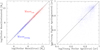 |
Fig. 7 Comparison of the input true parameters with the output estimated parameters from the mock catalog created by CIGALE. Only mass and age, the two main parameters of immediate interest, are shown. Left panel: stellar masses: blue points are the masses of the young stellar component. Red points are the masses of the old stellar component (in our case Massold + Massintermediate). Right panel:young stellar age. The solid line is the 1:1 relation in both panels. |
4.1 Equivalent width correction (the fr factor)
The observed equivalent width of Hβ, EW(Hβ), has been shown to be an indication of the age of the burst for young stellar systems (Dottori 1981).
From a sample of HII galaxies, Terlevich et al. (2004) showed that the observed distribution of EW(Hβ) cannot be reproduced if the evolution of the starburst is represented by a simple stellar population (SSP) predicted by evolutionary population synthesis models such as Starburst 99 (Leitherer et al. 1999). The very high EW(Hβ)young predicted for a very young stellar cluster is never observed, indicating that the observed EW(Hβ)obs is actually a measure of the intensity of the Hβ emission line (F(Hβ)) produced bythe young burst averaged by the past history of star formation, including the continuum emission of the young massive star cluster (Cyoung) plus the continuum emission produced by the previous episodes of star formation (Cold). Hence,
 (2)
(2)
We thus define the fraction fr as the ratio  , so
, so
 (3)
(3)
Figure 8 (left panel) shows the derived equivalent width correction factor (1 + fr) from Eq. (3). The resulting equivalent width distributions are given in Fig. 8 (right panel). The corrected  (blue histogram) is then the true equivalent width to be assigned to determine the burst ages using Eq. (3), where fr is derived from the SED fitting. The median value of the equivalent width correction factor from Eq. (3) is 1 + fr = 2.0.
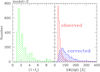 |
Fig. 8 EW(Hβ) correction factor fr (left). Histogram of the distributions of equivalent widths of Hβ (right). The red histogram shows the observed values from SDSS spectra. The blue histogram is the corrected EW(Hβ) for the contribution of an underlying old stellar population using the results from the SED fitting as described in the text. |
4.2 Relation between luminosity and young stellar mass
It is notoriously difficult to estimate the uncertainties of the parameters resulting from population synthesis models. Statistical errors in CIGALE are estimated through Bayesian probability distribution functions and are given for each output parameter. Typical errors for the masses in our work are in the range 20–30%, and for SFR errors are estimated to be 30–40%.
A straightforward way of verifying our results is to compare the mass of young stars, Myoung, from CIGALE with the observed Hβ luminosities, L(Hβ). This comparison is presented in Fig. 9 and shows an excellent correlation between these parameters. It should be noted, however, that since mass and luminosity depend on the square of the distance, the slope of a log-log plot such as this one is expected to be close to unity even when the objects span a relatively small range of distances, so the interesting information is in the scatter and the zero point, but not necessarily in the slope.
The ionizing fluxes of single-age (simple) starbursts depend mostly on two parameters: the age and the mass of the ionizing stars, and for these objects the equivalent width of the Balmer lines provides a robust age indicator (Leitherer et al. 1999, henceforth SB99). Thus, we expect the scatter in the relation between Myoung and L(Hβ) to be correlated with EW(Hβ). Figure 9 shows that this is indeed the case. Objects with EW(Hβ) lower than average lie predominantly below the fit line, while objects with values above average are above the line. We note that the ridge separating these two groups is tilted relative to the least-squares fit.
In the figure we used the equivalent widths corrected for contamination by old stars as described in Sect. 4.1, but the separation also occurs when the uncorrected EW(Hβ) are used, albeit with larger scatter and more overlap between the two groups (cf. Table 5 below).
In Melnick et al. (2017) we showed how the SB99 models can be used to normalize the observed Hβ luminosities to a fiducial age. Here we have used a dense grid of SB99 models for the standard Geneva isochrones with a metallicity of Z = 0.008 and a Kroupa IMF shown in Fig. 10. This allows us to directly interpolate the models to the observed EW(Hβ) without recourse to fitting analytic expressions, as in Melnick et al. (2017) or Fernández-Arenas et al. (2018).
Thus, for each object in our sample we interpolated the SB99 models to retrieve the luminosity offset between the observed age and the fiducial age, for which we chose the mean age of the sample, and we scaled the corrected luminosity to the actual mass (Myoung) of the object. For the SB99 models that we are using here the mean equivalent width of our sample corrected for contamination by old stars ⟨EW(Hβ)⟩ = 110.4 Å corresponds to a mean age of 3.8 Myr. Figure 11 shows the relation between young stellar mass and Hβ luminosity at a fiducial age of 3.8 Myr.
The scatter is significantly reduced while the stratification of luminosities as a function of EW(Hβ) is gone. Interestingly, however, the figure shows a systematic trend of EW(Hβ) with mass: massive objects tendto have lower equivalent widths. The figure also shows that simple SB99 models predict significantly higher luminosities than observed, and that therelation using corrected luminosities is steeper than the uncorrected case (Fig. 9). We find, therefore, that single-age models provide the correct slopes (d logL∕dEW) of the evolutionary corrections, but not the correct zero points.
Simple dynamical arguments indicate that very massive strictly coeval (simple) starburst clusters cannot exist. The characteristic timescales for the formation of such clusters would be toolong compared to the main-sequence lifetimes of the ionizing stars. So it is reasonable to assume that the stars in massive starbursts span a range of ages that is significant relative to the ages of the ionizing stars. In fact, observations of nearby HII Galaxies show that these objects tend to be clumpy and have multiple emission line profiles (Lagos et al. 2011; Melnick et al. 2017).
In order to test this multiplicity effect we performed simple Monte Carlo experiments where we split the young component of each galaxy with Myoung > 3 × 10⁶ M⊙ into a set of clumps of masses Mcl randomly sampled from a power-law mass distribution of slope α = −2 in the range 3 × 10⁵ < Mcl∕M⊙ < 3 × 10⁶. We then assigned to each clump a random age sampled from a Gaussian distribution centered at the mean age of the galaxy (from EW(Hβ)young) with a dispersion that is a function of total young stellar mass: 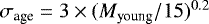 Myr, with Myoung in units of 106 M⊙. This generates a 3D grid from which we can read the predicted luminosity for a given mass and equivalent width.
The orange line in Fig. 11 illustrates the predictions from our simple Monte Carlo sampling. The prediction has the right slope, but is still offset by about 0.3 dex relative to the observations. It may be possible that more refined models could explain this offset, but a full sampling of parameter space is beyond the scope of this paper. For our immediate purposes, the important result is that simple SB99 models are adequate for estimating the evolutionary corrections to the Hβ luminosities of young starbursts.
In Table 5 we explore possible additional sources of systematic scatter in the L(Hβ) – Myoung relation. The evolutionary corrections parametrized by the raw equivalent widths is shown in the first line, and the corrected evolutionary corrections for contamination by old stars in the second line. The rest of the table explores the scatter of the age-corrected mass-luminosity relation discussed above (Fig. 11).
We find a weak correlation with nebular excitation ([OIII]/[OII]), which is probably a residual from our evolutionary corrections. The decrease in scatter is deceiving because, as shown in Fig. 11, when the luminosities are corrected for evolution using the SB99 models the scatter is rms = 0.22. Also, the 1965 galaxies with measured [OII]3727 Å tend to be those with the best S/N. We do not see any residual correlation with metallicity or [OIII]/Hβ. We conclude, therefore, that to a very good approximation, the Hβ luminosities of HII Galaxies depend only on two parameters: the mass and the age of the starburst component. An immediate corollary of this conclusion is that the IMF of HII Galaxies is universal, at least for massive stars.
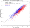 |
Fig. 9 Relation between young stellar mass from CIGALE (Myoung) and the observed Hβ luminosity for our sample of 2234 HII Galaxies with accurate SED fits (χ2 < 3). The sample was divided into two groups according to their equivalent widths, EW(Hβ), corrected for contamination as described in Sect. 4.1. Objects in red have EW(Hβ) lower than the average of the sample (110 Å) while objects in blue have values above the average. The line shows a standard least-squares fit of slope very close to unity, as indicated in the legend. Typical error in Myoung is < 30%. |
Multi-parametric fits.
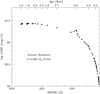 |
Fig. 10 Relation between L(Hβ) and EW(Hβ) for a simple 106 M⊙ starburst of Kroupa IMF (from SB99). The age scale is shown at the top of the figure. |
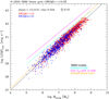 |
Fig. 11 Relation between young stellar mass from CIGALE (Myoung) and Hβ luminosity at a fiducial age of 3.8 Myr. As in Fig. 9, the sample was split into two groups according to the corrected equivalent widths. We show in red objects with less than the average of the sample (110 Å) and in blue objects with higher values. The colored lines show the predictions of SB99 models for two different stellar models as indicated in the figure. The orange line corresponds to the Monte Carlo sampling discussed in the text. |
4.3 The most massive starbursts
We remarked above that Fig. 11 shows a clear systematic decrease in EW(Hβ) with young stellar mass, in the sense that the most massive objects tend to have the lowest equivalent widths. The galaxies in our sample show a rather weak trend of metallicity with Myoung for low-mass objects, while the most massive starbursts span the full range of metallicities, so even after correction for underlying older stellar populations, we were puzzled by the fact that the most massive objects in our sample are still those with the lowest EW(Hβ).
Visual inspection of the SDSS images revealed that most of these massive HII Galaxies show disturbed morphologies reminiscent of major mergers. Thus, the most luminous objects in our sample seem to be the low-mass equivalents of LIRGS and ULIRGS, the descendants of mergers of massive spiral galaxies.
It is interesting to note in this context that the relation between age dispersion and mass ( ) from our Monte Carlo experiments is flatter than we expect from the Virial theorem and the L-σ relation,
 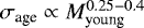 . This may be an indication that mergers rather than monolithic collapse controls the age spread in the most massive objects. Rejuvenation of massive stars through binary interactions may also play a role, although clearly more elaborate models are required to address these issues properly.
4.4 Stellar masses and star formation
Figure 12 shows histograms of indicators of the importance of the current star formation (SF) episode over the past history of star formation from our SED fitting. The left panel shows the histograms of the derived masses for the young stellar component (Myoung < 10 Myr) compared with the old stellar component (Mold = Mint + M10Gy). We note that we are not making a distinction in our CIGALE models between mass produced in the intermediate-age episode (Mint) from the mass of first episode of star formation (M10Gy) in our three burst model, so we refer to these two components simply as Mold.
We can see that our galaxies have total masses of less than 1010 M⊙, and typically 109 M⊙, putting them in the low-mass tail of other studies of overall properties of star-forming galaxies. This is of course due to our selection criteria, as explained in Sect. 2.
The middle panel shows the strength of the burst parameter defined as  . It is clear from this histogram that the present episode of SF has contributed very little to the total stellar mass production over the lifetime of these galaxies, typically less than 2%. Analogously, the right panel shows the b parameter (Kennicutt 1983), here defined as the ratio of the present-day SFR (SFR10My) to the average past SFR (SFR10Gy). The current star formation is producing stars at high rates, typically over ~20 times the average past history.
Our SED fitting procedure allows us to isolate the mass of the young stellar component produced in the latest SF episode (Myoung). Thus, the current SFR10My is simply Myoung/age10My. We used the actual CIGALE best fitting young ages of the individual objects, although there would have been little difference even if we had used the mean age for our sample of ⟨ log(age)10My ⟩ = 6.8, or a more conservative maximum age for the ionizing population of log(age)10My = 7. For the SFR averaged over the whole SFH of the galaxy SFR10Gy we take Mold∕1010 yr.
Figure 13 shows our current SFR derived from our SED fitting procedure log (SFR10My), plotted against our observed Hβ luminosities corrected for extinction (see Sect. 2). The resulting calibration forcing the slope to be exactly one is given by
 (4)
(4)
For comparison, the commonly used calibration of Kennicutt (1998), shown as the green line in the figure, is log (SFR) = −40.65 + logL(Hβ). The difference inzero point is only partially due to a slightly different IMF, stellar input in the synthesis model, or aperture effects, and mostly to the fact that our calibration isolates the SFR of the starburst component alone. Thus, the Kennicutt relation underestimates the present SFR of starbursts typically by a factor of 3. The prototypical starburst 30 Dor in the LMC is seen to fall exactly within the errors in the locus of HII galaxies (see Fig. 13) confirming that the starbursts in HII galaxies are similar to the Giant HII Regions in local spiral and irregular galaxies.
The relation between SFR and stellar mass is generally known as the main sequence of star-forming galaxies. There are extensive discussions of this relation in the literature and its use as a probe of galaxy evolution as a function of mass, environment, and galaxy types (Pérez-González et al. 2003; Brinchmann et al. 2004; Noeske et al. 2007; Salim et al. 2007; Daddi et al. 2007; Elbaz et al. 2007; Peng et al. 2010; Chang et al. 2015; Salim et al. 2016), as well as subsets of extremely metal-poor galaxies (Filho et al. 2016, and references therein) and samples of BCDs (Sánchez Almeida et al. 2009; Izotov et al. 2014; Janowiecki et al. 2017). Various SFR indicators have been used, but Kennicutt’s Hα luminosity is the most common indicator for local star-forming galaxies (Kennicutt 1983; Brinchmann et al. 2004).
Figure 14 (left panel) plots the relationship between the SFR derived from our calibration given by Eq. (4) and stellar masses for our sample. The relation for the total masses shown by the red points and red line is given by
 (5)
(5)
with an rms = 0.313. For comparison, we plot the relation derived from other commonly used samples of star-forming galaxies in the literature. The green and cyan lines are from Chang et al. (2015). The latter represents their calibration using the values from Brinchmann et al. (2004) for stellar masses and SFRs. The orange line is from Elbaz et al. (2007) for their sample of blue star-forming galaxies. Even considering the scatter in these relations it is clear that the main sequence of HII galaxies (red points) is significantly steeper and stronger than the relation for more general samples of star-forming galaxies.
The blue points in the figure show the SFR for the starburst component alone. A linear fit (blue line) to this relation gives
 (6)
(6)
with an rms = 0.297. This relation can be interpreted as the empirically derived main sequence for single starbursts and represents the maximum star formation rates for starbursts.
To illustrate this point, Fig. 14 (right panel) shows the relation between what is known as the specific star formation rate (sSFR), which is the star formation rate per unit mass, as a function of stellar mass. As in the previous figure, the blue points represent the star formation per unit mass of stars formed in the current star formation episode (Myoung) and the redpoints represent the current star formation rate over all stars (Mtotal) formed in the past history of the galaxy. HII Galaxies fall well above the overall average for star-forming galaxies of log(sSFR) ~ –10 yr−1 (Guo et al. 2015).
Averaged over their entire lifetimes HII Galaxies have thus been forming stars at levels that approach the largest starburst galaxies such as ULIRGS represented in the figure by Arp 220 with log(sSFR) ~ –8 yr−1. However, if we consider the sSFR of the present burst alone (SFR per unit of young population stellar mass), the current starbursts in HII Galaxies are producing new stars at a much higher rate of log(sSFR) ~ –7 to –6.5 yr−1. By the same token, the present-day sSFR of ULIRGS are close to the upper limit set by HII galaxies when normalized by their young population stellar masses.
Figure 14 also shows the SFR (left panel) and sSFR (right panel) for the prototypical Giant HII Region 30 Doradus in the LMC. Doran et al. (2013) derived a mass of 1.1 × 10⁵ M⊙ and a SFR of 0.073 ± 0.04 M⊙ yr−1 for a Kroupa IMF from their stellar Lyman continuum census. Although star formation in 30 Dor has spread over 5 Myr (Selman et al. 1999), this is the closest example of a genuine real-life simple young massive stellar population, and sets an upper limit to how fast star formation may occur in starbursts. The purple dashed line in Fig. 14 (right panel) shows the “speed limit” for star formation that is set by 30 Dor.
As discussed above, simple dynamical arguments imply that objects substantially more massive than 30 Doradus, which is the case for all the HII Galaxies in our sample, cannot form stars significantly faster than 30 Dor. This also explains the declining tilt of the sSFR of our galaxies shown in the figure: only low-mass HII Galaxies can harbor the most intense starbursts.
 |
Fig. 12 Young stellar mass (blue) and old stellar mass (red) (left). Burst strength ( |

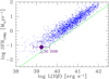 |
Fig. 13 SFR vs. LHβ calibration. The blue points are for the current star formation rate from SED result of SFR10My = Myoung∕ageyoung (⟨ age⟩young = 6.8 My). The green line is the relation by Kennicutt (1998) for normal spiral galaxies. The purple hexagon is the giant HII region 30 Dor in the LMC (Doran et al. 2013; Crowther et al. 2017). |
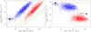 |
Fig. 14 Left panel: main sequence of HII galaxies: current SFR derived from the calibration between our SFR averaged over 10 Myr from our SED fitting procedure vs. the LHβ from Eq. (4), as a function of Massyoung (blue points and line) and of Masstotal (red points and line). The green line is from Brinchmann et al. (2004), the cyan line from Chang et al. (2015), and the orange line from Elbaz et al. (2007; see text). Right panel: specific SFR as a function of stellar mass, as in the left panel. In both plots the positions of the genuine starburst 30 Dor in the LMC are given (magenta). The black point in the right panel represents the position of the ULIRG Arp 220 with SFR over ~200 M⊙yr−1. |
4.5 The L-σ relation
The strong relation between L(Hβ) and Myoung found in this paper confirms that the L-σ relation is indeed a correlation between the mass of the starburst component and the turbulence of the ionized gas. However, the relation remains empirical because we do not yet fully understand the origin of the gas turbulence in HII Galaxies. It could be due to gravity, if the gas clouds are virialized, or to the direct injection of mechanical energy from massive stars via stellar winds, or a combinationof both.
We used the fr factors derived from our SED fitting to correct the luminosities of the galaxies used in Melnick et al. (2017) to study the scatter of the relation and found that the corrections actually increase the scatter quite substantially. This is probably due to the fact that the corrections expose the effect of a second parameter, possibly associated with the effective radius of the young component (R), as expected if the gas is virialized (Chávez et al. 2016). Unfortunately, however, good measurements of the effective radii of these galaxies are not yet available to verify, for example, whether Rσ2 correlates with Myoung as expected if the gas is in virial equilibrium with the stellar potential.
5 Concluding remarks
We have studied a representative sample of the youngest (⟨EW(Hβ)⟩ = 50Å), highest excitation, and lowest metallicity (⟨ 12+logO/H ⟩ = 8.2) HII Galaxies in the local universe (z < 0.4) and find that, as a class, they have the following properties:
- 1.
The correction factor (1 + fr) is typically between 1.5 and 2.5. This factor is derived from our SED fitting procedure and is then applied on the observedEW(Hβ) in order to correct for the contribution of the underlying old stellar continuum and recover the true
 .
. - 2.
The star formation histories of HII Galaxies can be reproduced remarkably well by three bursts of star formation: (a) the current young burst, a few Myr old, that dominates the luminosity at all wavelengths, but contains only a small percent of the total mass; (b) an intermediate-age burst of a few hundred Myr; (c) and an old stellar component (10 Gyr). The intermediate-age burst and the old burst together contain most of the mass. Therefore, the past SFH is far more important in producing the bulk of the stellar mass in HII galaxies.
- 3.
At a given age, the Hβ luminosity of HII Galaxies depends only on the mass of young stars. This implies that the IMF of the ionizing clusters must be a universal function at least for massive stars, and that only a relatively small fraction of Lyman continuum photons escape from the nebulae (case B photoionization).
- 4.
The main sequence of star formation for HII Galaxies is significantly steeper and stronger than that of more massive star-forming galaxies from the literature, while the present-day star formation rates of HII Galaxies are on average a factor of three higher than predicted by the Hα Kennicutt relation. Therefore, extreme care must be exercised when combining starburst galaxies with more normal galaxies to construct the overall main sequence of star-forming galaxies.
Acknowledgments
We are grateful to Denis Burgarella, the father of CIGALE, and to Médéric Boquien for guiding us through our first steps with the code and answering numerous questions. Médéric kindly wrote the special module to fit the three stellar populations that were used in this work. ET thanks Roderik Overzier for fruitful discussions, and Elena Terlevich for comments on the manuscript. JM acknowledges support from a CNPq Ciencia Sem Fronteiras grant at the Observatorio Nacional in Rio de Janeiro, and the hospitality of ON as a PVE visitor. Finally, we thank the anonymous referee for the comments and suggestions that improved the paper. Funding for the SDSS and SDSS-II has been provided by the Alfred P. Sloan Foundation, the Participating Institutions, the National Science Foundation, the U.S. Department of Energy, the National Aeronautics and Space Administration, the Japanese Monbukagakusho, the Max Planck Society, and the Higher Education Funding Council for England. The SDSS Web Site is http://www.sdss.org/. The SDSS is managed by the Astrophysical Research Consortium for the Participating Institutions. The Participating Institutions are the American Museum of Natural History, Astrophysical Institute Potsdam, University of Basel, University of Cambridge, Case Western Reserve University, University of Chicago, Drexel University, Fermilab, the Institute for Advanced Study, the Japan Participation Group, Johns Hopkins University, the Joint Institute for Nuclear Astrophysics, the Kavli Institute for Particle Astrophysics and Cosmology, the Korean Scientist Group, the Chinese Academy of Sciences (LAMOST), Los Alamos National Laboratory, the Max-Planck-Institute for Astronomy (MPIA), the Max-Planck-Institute for Astrophysics (MPA), New Mexico State University, The Ohio State University, University of Pittsburgh, University of Portsmouth, Princeton University, the United States Naval Observatory, and the University of Washington. The entire GALEX Team gratefully acknowledges NASA’s support for the construction, operation, and science analysis of the GALEX mission, developed in corporation with the Centre National d’Études Spatiales of France and the Korean Ministry of Science and Technology. We acknowledge the dedicated team of engineers, technicians, and administrative staff from JPL/Caltech, Orbital Sciences Corporation, University of California, Berkeley, Laboratoire d’Astrophysique Marseille, and the other institutions who made this mission possible. The UKIDSS project is defined in Lawrence et al. (2007). UKIDSS uses the UKIRT Wide Field Camera WFCAM (Casali et al. 2007). The photometric system is described in Hewett et al. (2006), and the calibration is described in Hodgkin et al. (2009). The pipeline processing and science archive are described in Irwin et al. (in prep.) and Hambly et al. (2008). This publication makes use of data products from the Wide-field Infrared Survey Explorer, which is a joint project of the University of California, Los Angeles, and the Jet Propulsion Laboratory/California Institute of Technology, funded by the National Aeronautics and Space Administration.
References
- Albareti, F. D., Allende Prieto, C., Almeida, A., et al. 2017, ApJS, 233, 25[0pc] [NASA ADS] [CrossRef] [Google Scholar]
- Baldwin, J. A., Phillips, M. M., & Terlevich, R. 1981, PASP, 93, 5 [NASA ADS] [CrossRef] [EDP Sciences] [Google Scholar]
- Bianchi, L. 2014, Ap&SS, 354, 103 [NASA ADS] [CrossRef] [Google Scholar]
- Boquien, M., Buat, V., & Perret, V. 2014, A&A, 571, A72 [NASA ADS] [CrossRef] [EDP Sciences] [Google Scholar]
- Boquien, M., Kennicutt, R., Calzetti, D., et al. 2016, A&A, 591, A6 [NASA ADS] [CrossRef] [EDP Sciences] [Google Scholar]
- Bordalo, V., & Telles, E. 2011, ApJ, 735, 52 [NASA ADS] [CrossRef] [Google Scholar]
- Bordalo, V., Plana, H., & Telles, E. 2009, ApJ, 696, 1668 [NASA ADS] [CrossRef] [Google Scholar]
- Brinchmann, J., Charlot, S., White, S. D. M., et al. 2004, MNRAS, 351, 1151 [NASA ADS] [CrossRef] [Google Scholar]
- Bruzual, G., & Charlot, S. 2003, MNRAS, 344, 1000 [NASA ADS] [CrossRef] [Google Scholar]
- Buat, V., Giovannoli, E., Takeuchi, T. T., et al. 2011, A&A, 529, A22 [NASA ADS] [CrossRef] [EDP Sciences] [Google Scholar]
- Calzetti, D., Armus, L., Bohlin, R. C., et al. 2000, ApJ, 533, 682 [NASA ADS] [CrossRef] [Google Scholar]
- Cappellari, M., & Emsellem, E. 2004, PASP, 116, 138 [NASA ADS] [CrossRef] [Google Scholar]
- Cardamone, C., Schawinski, K., Sarzi, M., et al. 2009, MNRAS, 399, 1191 [NASA ADS] [CrossRef] [Google Scholar]
- Cardelli, J. A., Clayton, G. C., & Mathis, J. S. 1989, ApJ, 345, 245 [NASA ADS] [CrossRef] [Google Scholar]
- Casali, M., Adamson, A., Alves de Oliveira, C., et al. 2007, A&A, 467, 777 [NASA ADS] [CrossRef] [EDP Sciences] [Google Scholar]
- Chang, Y.-Y., van der Wel, A., da Cunha, E., & Rix, H.-W. 2015, ApJS, 219, 8 [NASA ADS] [CrossRef] [Google Scholar]
- Chávez, R., Terlevich, R., Terlevich, E., et al. 2014, MNRAS, 442, 3565 [NASA ADS] [CrossRef] [Google Scholar]
- Chávez, R., Plionis, M., Basilakos, S., et al. 2016, MNRAS, 462, 2431 [NASA ADS] [CrossRef] [Google Scholar]
- Ciesla, L., Charmandaris, V., Georgakakis, A., et al. 2015, A&A, 576, A10 [NASA ADS] [CrossRef] [EDP Sciences] [Google Scholar]
- Ciesla, L., Boselli, A., Elbaz, D., et al. 2016, A&A, 585, A43 [NASA ADS] [CrossRef] [EDP Sciences] [Google Scholar]
- Crowther, P., Caballero-Nieves, S., Castro, N., & Evans, C. 2017, IAU Symp., 329, 292 [NASA ADS] [Google Scholar]
- Curti, M., Cresci, G., Mannucci, F., et al. 2017, MNRAS, 465, 1384 [NASA ADS] [CrossRef] [Google Scholar]
- Daddi, E., Dickinson, M., Morrison, G., et al. 2007, ApJ, 670, 156 [NASA ADS] [CrossRef] [Google Scholar]
- Dale, D. A., Helou, G., Magdis, G. E., et al. 2014, ApJ, 784, 83 [NASA ADS] [CrossRef] [Google Scholar]
- Debsarma, S., Chattopadhyay, T., Das, S., & Pfenniger, D. 2016, MNRAS, 462, 3739 [NASA ADS] [CrossRef] [Google Scholar]
- Doran, E. I., Crowther, P. A., de Koter, A., et al. 2013, A&A, 558, A134 [NASA ADS] [CrossRef] [EDP Sciences] [Google Scholar]
- Dottori, H. A. 1981, Ap&SS, 80, 267 [NASA ADS] [CrossRef] [Google Scholar]
- Draine, B. T.,& Li, A. 2007, ApJ, 657, 810 [NASA ADS] [CrossRef] [Google Scholar]
- Elbaz, D., Daddi, E., Le Borgne, D., et al. 2007, A&A, 468, 33 [NASA ADS] [CrossRef] [EDP Sciences] [Google Scholar]
- Elmegreen, D. M., Elmegreen, B. G., Sánchez Almeida, J., et al. 2012, ApJ, 750, 95 [NASA ADS] [CrossRef] [Google Scholar]
- Fernández-Arenas, D., Terlevich, E., Terlevich, R., et al. 2018, MNRAS, 474, 1250 [NASA ADS] [CrossRef] [Google Scholar]
- Filho, M. E., Sánchez Almeida, J., Amorín, R., et al. 2016, ApJ, 820, 109 [NASA ADS] [CrossRef] [Google Scholar]
- Giovannoli, E., Buat, V., Noll, S., Burgarella, D., & Magnelli, B. 2011, A&A, 525, A150 [NASA ADS] [CrossRef] [EDP Sciences] [Google Scholar]
- Gordon, K. D., Calzetti, D., & Witt, A. N. 1997, ApJ, 487, 625 [NASA ADS] [CrossRef] [Google Scholar]
- Gordon, K. D., Clayton, G. C., Misselt, K. A., Landolt, A. U., & Wolff, M. J. 2003, ApJ, 594, 279 [NASA ADS] [CrossRef] [EDP Sciences] [Google Scholar]
- Guo, K., Zheng, X. Z., Wang, T., & Fu, H. 2015, ApJ, 808, L49 [NASA ADS] [CrossRef] [Google Scholar]
- Hambly, N. C., Collins, R. S., Cross, N. J. G., et al. 2008, MNRAS, 384, 637 [NASA ADS] [CrossRef] [Google Scholar]
- Hewett, P. C., Warren, S. J., Leggett, S. K., & Hodgkin, S. T. 2006, MNRAS, 367, 454 [NASA ADS] [CrossRef] [Google Scholar]
- Hewett, P. C., Warren, S. J., Leggett, S. K., & Hodgkin, S. T. 2006, MNRAS, 367, 454 [NASA ADS] [CrossRef] [Google Scholar]
- Hodgkin, S. T., Irwin, M. J., Hewett, P. C., Warren, S. J. 2009, MNRAS, 394, 675 [NASA ADS] [CrossRef] [Google Scholar]
- Izotov, Y. I., Stasińska, G., Meynet, G., Guseva, N. G., & Thuan, T. X. 2006, A&A, 448, 955 [NASA ADS] [CrossRef] [EDP Sciences] [Google Scholar]
- Izotov, Y. I., Guseva, N. G., Fricke, K. J., & Henkel, C. 2014, A&A, 561, A33 [NASA ADS] [CrossRef] [EDP Sciences] [Google Scholar]
- Izotov, Y. I., Thuan, T. X., Guseva, N. G., & Liss, S. E. 2018, MNRAS, 473, 1956 [NASA ADS] [CrossRef] [Google Scholar]
- Janowiecki, S., Salzer, J. J., van Zee, L., Rosenberg, J. L., & Skillman, E. 2017, ApJ, 836, 128 [NASA ADS] [CrossRef] [Google Scholar]
- Kauffmann, G., Heckman, T. M., Tremonti, C., et al. 2003, MNRAS, 346, 1055 [Google Scholar]
- Kehrig, C., Telles, E., & Cuisinier, F. 2004, AJ, 128, 1141 [NASA ADS] [CrossRef] [Google Scholar]
- Kennicutt, Jr. R. C. 1983, ApJ, 272, 54 [NASA ADS] [CrossRef] [EDP Sciences] [Google Scholar]
- Kennicutt, Jr. R. C. 1998, ARA&A, 36, 189 [Google Scholar]
- Kewley, L. J., Groves, B., Kauffmann, G., & Heckman, T. 2006, MNRAS, 372, 961 [NASA ADS] [CrossRef] [Google Scholar]
- Kunth, D., & Östlin, G. 2000, A&ARv, 10, 1 [NASA ADS] [CrossRef] [Google Scholar]
- Kunth, D., Maurogordato, S., & Vigroux, L. 1988, A&A, 204, 10 [NASA ADS] [Google Scholar]
- Lagos, P., Telles, E., & Melnick, J. 2007, A&A, 476, 89 [NASA ADS] [CrossRef] [EDP Sciences] [Google Scholar]
- Lagos, P., Telles, E., Nigoche-Netro, A., & Carrasco, E. R. 2011, AJ, 142, 162 [NASA ADS] [CrossRef] [Google Scholar]
- Lawrence, A., Warren, S. J., Almaini, O., et al. 2007, MNRAS, 379, 1599 [NASA ADS] [CrossRef] [MathSciNet] [Google Scholar]
- Leitherer, C., Schaerer, D., Goldader, J. D., et al. 1999, ApJS, 123, 3 [NASA ADS] [CrossRef] [Google Scholar]
- Leitherer, C., Calzetti, D., & Martins, L. P. 2002, ApJ, 574, 114 [NASA ADS] [CrossRef] [Google Scholar]
- Loose, H.-H., & Thuan, T. X. 1986, in Star-forming Dwarf Galaxies and Related Objects, eds. D. Kunth, T. X. Thuan, J. Tran Thanh Van, J. Lequeux, & J. Audouze, 73 [Google Scholar]
- Melnick, J., Terlevich, R., & Moles, M. 1988, MNRAS, 235, 297 [NASA ADS] [CrossRef] [Google Scholar]
- Melnick, J., Terlevich, R., & Terlevich, E. 2000, MNRAS, 311, 629 [NASA ADS] [CrossRef] [Google Scholar]
- Melnick, J., Telles, E., Bordalo, V., et al. 2017, A&A, 599, A76 [NASA ADS] [CrossRef] [EDP Sciences] [Google Scholar]
- Noeske, K. G., Weiner, B. J., Faber, S. M., et al. 2007, ApJ, 660, L43 [Google Scholar]
- Noll, S., Burgarella, D., Giovannoli, E., et al. 2009, A&A, 507, 1793 [NASA ADS] [CrossRef] [EDP Sciences] [Google Scholar]
- Osterbrock, D. E. 1989, Astrophysics of gaseous nebulae and active galactic nuclei (Mill Valley: University Science Books) [CrossRef] [Google Scholar]
- Pagel, B. E. J., Simonson, E. A., Terlevich, R. J., & Edmunds, M. G. 1992, MNRAS, 255, 325 [NASA ADS] [CrossRef] [Google Scholar]
- Papaderos, P., Guseva, N. G., Izotov, Y. I., & Fricke, K. J. 2008, A&A, 491, 113 [NASA ADS] [CrossRef] [EDP Sciences] [Google Scholar]
- Pelupessy, F. I., van der Werf, P. P., & Icke, V. 2004, A&A, 422, 55 [NASA ADS] [CrossRef] [EDP Sciences] [Google Scholar]
- Peng, Y.-j., Lilly, S. J., Kovač, K., et al. 2010, ApJ, 721, 193 [NASA ADS] [CrossRef] [Google Scholar]
- Pérez-González, P. G., Zamorano, J., Gallego, J., Aragón-Salamanca, A., & Gil de Paz, A. 2003, ApJ, 591, 827 [NASA ADS] [CrossRef] [Google Scholar]
- Plionis, M., Terlevich, R., Basilakos, S., et al. 2011, MNRAS, 416, 2981 [NASA ADS] [CrossRef] [Google Scholar]
- Salim, S., Rich, R. M., Charlot, S., et al. 2007, ApJS, 173, 267 [NASA ADS] [CrossRef] [Google Scholar]
- Salim, S., Lee, J. C., Janowiecki, S., et al. 2016, ApJS, 227, 2 [NASA ADS] [CrossRef] [Google Scholar]
- Sánchez Almeida, J., Aguerri, J. A. L., Muñoz-Tuñón, C., & Vazdekis, A. 2009, ApJ, 698, 1497 [NASA ADS] [CrossRef] [Google Scholar]
- Sargent, W. L. W., & Searle, L. 1970, ApJ, 162, L155 [NASA ADS] [CrossRef] [Google Scholar]
- Sarzi, M., Falcón-Barroso, J., Davies, R. L., et al. 2006, MNRAS, 366, 1151 [NASA ADS] [CrossRef] [Google Scholar]
- Albareti, F. D., Allende Prieto, C., Almeida, A., et al. 2017, ApJS, 233, 25 [NASA ADS] [CrossRef] [Google Scholar]
- Schlafly, E. F., & Finkbeiner, D. P. 2011, ApJ, 737, 103 [NASA ADS] [CrossRef] [Google Scholar]
- Selman, F., Melnick, J., Bosch, G., & Terlevich, R. 1999, A&A, 347, 532 [NASA ADS] [Google Scholar]
- Stasińska, G., Cid Fernandes, R., Mateus, A., Sodré, L., & Asari, N. V. 2006, MNRAS, 371, 972 [NASA ADS] [CrossRef] [Google Scholar]
- Telles, E., & Terlevich, R. 1993, Ap&SS, 205, 49 [NASA ADS] [CrossRef] [Google Scholar]
- Telles, E., & Terlevich, R. 1997, MNRAS, 286, 183 [NASA ADS] [CrossRef] [Google Scholar]
- Telles, E., Melnick, J., & Terlevich, R. 1997, MNRAS, 288, 78 [NASA ADS] [CrossRef] [Google Scholar]
- Terlevich, R., & Melnick, J. 1981, MNRAS, 195, 839 [NASA ADS] [CrossRef] [Google Scholar]
- Terlevich, R., Melnick, J., Masegosa, J., Moles, M., & Copetti, M. V. F. 1991, A&AS, 91, 285 [NASA ADS] [Google Scholar]
- Terlevich, R., Silich, S., Rosa-González, D., & Terlevich, E. 2004, MNRAS, 348, 1191 [NASA ADS] [CrossRef] [Google Scholar]
- Terlevich, R., Terlevich, E., Melnick, J., et al. 2015, MNRAS, 451, 3001 [NASA ADS] [CrossRef] [Google Scholar]
- Thomas, D., Steele, O., Maraston, C., et al. 2013, MNRAS, 431, 1383 [NASA ADS] [CrossRef] [Google Scholar]
- Tremonti, C. A., Heckman, T. M., Kauffmann, G., et al. 2004, ApJ, 613, 898 [NASA ADS] [CrossRef] [Google Scholar]
- Vika, M., Ciesla, L., Charmandaris, V., Xilouris, E. M., & Lebouteiller, V. 2017, A&A, 597, A51 [NASA ADS] [CrossRef] [EDP Sciences] [Google Scholar]
- Westera, P., Cuisinier, F., Telles, E., & Kehrig, C. 2004, A&A, 423, 133 [NASA ADS] [CrossRef] [EDP Sciences] [Google Scholar]
- Wright, E. L., Eisenhardt, P. R. M., Mainzer, A. K., et al. 2010, AJ, 140, 1868 [NASA ADS] [CrossRef] [Google Scholar]
- York, D. G., Adelman, J., Anderson, Jr. J. E., et al. 2000, AJ, 120, 1579 [CrossRef] [Google Scholar]
The emissionLinePort table (Portsmouth stellar kinematics and emission line flux measurements; Thomas et al. 2013) is based on adaptations of the publicly available codes Penalized PiXel Fitting (pPXF; Cappellari & Emsellem 2004) and Gas and Absorption Line Fitting code (GANDALF v1.5; Sarzi et al. 2006) to calculate stellar kinematics and to derive emission line properties.
CIGALE software and documentation are available at: http://cigale.lam.fr/
All Tables
Summary of the selection criteria of our spectroscopic sample, resulting in our SDSS sample of ~4200 objects.
Number of objects that have the corresponding photometric data from the given surveys.
All Figures
|
Fig. 1 BPT diagram of the selected objects. The blue points are the whole sample of 67 000 starburst galaxies. The red points are the resulting spectroscopic sample of ~4200 galaxies with the criteria given in Table 1. HII galaxies lie below and to the left of the Kauffmann et al. (2003) classification (solid red line) that distinguishes AGNs from star-forming galaxies. |
| In the text | |
|
Fig. 2 Distribution of the Petrosian radius in the SDSS r band of our photometric sample of 2728 HII galaxies. The median value of the distribution is only 2.8′′. |
| In the text | |
|
Fig. 3 Spectroscopic properties of our sample of intense emission line objects. From left to right panels: distribution of the Balmer decrement derived extinction parameter, distribution of the equivalent width of Hβ, distribution of Hβ luminosity, and distribution of the oxygen abundance derived from the direct method for objects with the auroral [O III]λ4363 Å line detected. This line is detected virtually in all our galaxies and allows the determination of the electron temperature (see text). |
| In the text | |
|
Fig. 4 Balmer decrements for our sample relative to the theoretical Case B recombination values for Te = 11 400 K. The solid lines represent four different extinction laws as shown for a range of Δ AV = 1.4 mag. Points in gray are for the whole sample, while points in blue correspond to objects with errors in both axes < 0.015. The black cross at the bottom left represents the mean error of the whole sample. |
| In the text | |
|
Fig. 5 Comparing free fit without dust emission (left panel, MODEL 0) vs. with dust emission (right panel, MODEL 1). The Green points are the observed photometry from UV to MIR. Only the first two WISE data points are shown and used inthe fits. The solid lines are the modeled components: young stellar population (cyan), intermediate+old stellar population (orange), nebular continuum (magenta), and for MODEL 1 (right panel) the dust emission (red). The red points represent the model fit results for each photometric band. The information in the inset are the respective ages and derived masses of the stellar populations. The inset also shows the observed equivalent width of Hβ (WHβ) and the corrected equivalent width of Hβ for the young stellar component only (Wy(Hβ), see text.) |
| In the text | |
|
Fig. 6 Comparison of models 2 and 3 in relation to the residual of best fitted extinction parameter C( |
| In the text | |
|
Fig. 7 Comparison of the input true parameters with the output estimated parameters from the mock catalog created by CIGALE. Only mass and age, the two main parameters of immediate interest, are shown. Left panel: stellar masses: blue points are the masses of the young stellar component. Red points are the masses of the old stellar component (in our case Massold + Massintermediate). Right panel:young stellar age. The solid line is the 1:1 relation in both panels. |
| In the text | |
|
Fig. 8 EW(Hβ) correction factor fr (left). Histogram of the distributions of equivalent widths of Hβ (right). The red histogram shows the observed values from SDSS spectra. The blue histogram is the corrected EW(Hβ) for the contribution of an underlying old stellar population using the results from the SED fitting as described in the text. |
| In the text | |
|
Fig. 9 Relation between young stellar mass from CIGALE (Myoung) and the observed Hβ luminosity for our sample of 2234 HII Galaxies with accurate SED fits (χ2 < 3). The sample was divided into two groups according to their equivalent widths, EW(Hβ), corrected for contamination as described in Sect. 4.1. Objects in red have EW(Hβ) lower than the average of the sample (110 Å) while objects in blue have values above the average. The line shows a standard least-squares fit of slope very close to unity, as indicated in the legend. Typical error in Myoung is < 30%. |
| In the text | |
|
Fig. 10 Relation between L(Hβ) and EW(Hβ) for a simple 106 M⊙ starburst of Kroupa IMF (from SB99). The age scale is shown at the top of the figure. |
| In the text | |
|
Fig. 11 Relation between young stellar mass from CIGALE (Myoung) and Hβ luminosity at a fiducial age of 3.8 Myr. As in Fig. 9, the sample was split into two groups according to the corrected equivalent widths. We show in red objects with less than the average of the sample (110 Å) and in blue objects with higher values. The colored lines show the predictions of SB99 models for two different stellar models as indicated in the figure. The orange line corresponds to the Monte Carlo sampling discussed in the text. |
| In the text | |
|
Fig. 12 Young stellar mass (blue) and old stellar mass (red) (left). Burst strength ( |
| In the text | |
|
Fig. 13 SFR vs. LHβ calibration. The blue points are for the current star formation rate from SED result of SFR10My = Myoung∕ageyoung (⟨ age⟩young = 6.8 My). The green line is the relation by Kennicutt (1998) for normal spiral galaxies. The purple hexagon is the giant HII region 30 Dor in the LMC (Doran et al. 2013; Crowther et al. 2017). |
| In the text | |
|
Fig. 14 Left panel: main sequence of HII galaxies: current SFR derived from the calibration between our SFR averaged over 10 Myr from our SED fitting procedure vs. the LHβ from Eq. (4), as a function of Massyoung (blue points and line) and of Masstotal (red points and line). The green line is from Brinchmann et al. (2004), the cyan line from Chang et al. (2015), and the orange line from Elbaz et al. (2007; see text). Right panel: specific SFR as a function of stellar mass, as in the left panel. In both plots the positions of the genuine starburst 30 Dor in the LMC are given (magenta). The black point in the right panel represents the position of the ULIRG Arp 220 with SFR over ~200 M⊙yr−1. |
| In the text | |
Current usage metrics show cumulative count of Article Views (full-text article views including HTML views, PDF and ePub downloads, according to the available data) and Abstracts Views on Vision4Press platform.
Data correspond to usage on the plateform after 2015. The current usage metrics is available 48-96 hours after online publication and is updated daily on week days.
Initial download of the metrics may take a while.