| Issue |
A&A
Volume 615, July 2018
|
|
|---|---|---|
| Article Number | A109 | |
| Number of page(s) | 10 | |
| Section | Cosmology (including clusters of galaxies) | |
| DOI | https://doi.org/10.1051/0004-6361/201731212 | |
| Published online | 23 July 2018 | |
Spatial range of conformity
Ludwig–Maximilians Universtät München, Fakultät für Physik,
Schellingstr. 4,
80799
München, Germany
e-mail: This email address is being protected from spambots. You need JavaScript enabled to view it.
Received:
21
May
2017
Accepted:
23
March
2018
Abstract
Context. Properties of galaxies, such as their absolute magnitude and stellar mass content, are correlated. These correlations are tighter for close pairs of galaxies, which is called galactic conformity. In hierarchical structure formation scenarios, galaxies form within dark matter haloes. To explain the amplitude and spatial range of galactic conformity two-halo terms or assembly bias become important.
Aims. With the scale dependent correlation coefficients, the amplitude and spatial range of conformity are determined from galaxy and halo samples.
Methods. The scale dependent correlation coefficients are introduced as a new descriptive statistic to quantify the correlations between properties of galaxies or haloes, depending on the distances to other galaxies or haloes. These scale dependent correlation coefficients can be applied to the galaxy distribution directly. Neither a splitting of the sample into subsamples, nor an a priori clustering is needed.
Results. This new descriptive statistic is applied to galaxy catalogues derived from the Sloan Digital Sky Survey III and to halo catalogues from the MultiDark simulations. In the galaxy sample the correlations between absolute magnitude, velocity dispersion, ellipticity, and stellar mass content are investigated. The correlations of mass, spin, and ellipticity are explored in the halo samples. Both for galaxies and haloes a scale dependent conformity is confirmed. Moreover the scale dependent correlation coefficients reveal a signal of conformity out to 40 Mpc and beyond. The halo and galaxy samples show a differing amplitude and range of conformity.
Key words: large-scale structure of Universe / galaxies: statistics / galaxies: fundamental parameters / galaxies: formation
© ESO 2018
1 Introduction
The clustering of galaxies in space is an important observational constraint for models of structure formation in the Universe. Often galaxies are treated as points in space and one compares the clustering properties of this point distribution to models of structure formation. However galaxies are extended objects and come in various flavours. Their properties are categorised and quantified. One considers the luminosity, shape, substructure, or spectroscopic features of a galaxy to name only a few. As an extension, galaxies are still treated as points, but the properties of the galaxies are assigned to the points as marks. This establishes at each position of a galaxy a multi-dimensional space. Depending on the physical problem, various methods for the analysis of such a marked point set have been devised.
The concept of bias was developed to account for the stronger clustering of galaxy clusters compared to the clustering of galaxies themselves (Kaiser 1984; Bardeen et al. 1986). Currently bias is often used to describe the differences between the clustering of luminous and dark matter (see Desjacques et al. 2016 for a recent review)
With luminosity- and morphology-segregation one describes the differences in the spatial clustering of dim versus luminous galaxies, of early-type (e.g. ellipticals) versus late-type galaxies (e.g. spirals), or of red versus blue galaxies, etc. (Ostriker & Turner 1979; Hamilton 1988; Willmer et al. 1998). In most cases the ratios of the two-point correlation functions, determined from subsamples of the galaxy distribution are used to quantify these segregation effects (see e.g. Zehavi et al. 2011).
The morphology density relation indicates that early-type galaxies tend to reside in more dense environments compared to late-type galaxies. There are numerous observations confirming this (Dressler 1980; Postman & Geller 1984; Andreon et al. 1997; van der Wel et al. 2010). Effects of the morphology density relation are typically confined to groups and clusters of galaxies (see however Binggeli et al. 1990).
Conformity is an expression from sociology, it is the act of matching attitudes and behaviours to group norms. With galactic conformity one is investigating how strongly the properties of galaxies conform with each other, if they are located in a group around a bright dominating galaxy or in a dark matter halo (Weinmann et al. 2006). Galactic conformity is typically quantified by first determining the central galaxy within a group of galaxies. Then for example the fraction of late-type galaxies in the cluster is plotted against the mass of the group depending on the type of the central galaxy. Hence, galactic conformity is an extension of the morphology density relation with the bright central galaxy as the determinant for the galactic properties. This approach does not only use the types but also the colours, star formation rates, or other properties of the galaxies. Kauffmann et al. (2013) plotted the fraction of star-forming galaxies against the (projected) distance from the central galaxy, showing that conformity is scale dependent, at least on small scales. In hierarchical structure formation scenarios, galaxies form within dark matter haloes. To explain the amplitude and spatial range of galactic conformity two-halo terms or assembly bias becomes important. Using the halo model Hearin et al. (2015) were able to model such a scale dependence using two-halo conformity from assembly bias. A comparison of semi-analytic models reveals different patterns in the scale dependence of halo conformity between the models (see the discussion in Lacerna et al. 2018 and the references therein). Quantitative scale dependent methods are needed to discriminate these different approaches. This is especially important if one wishes to quantify the influence of large-scale structures on the conformity. Then one needs measures of conformity, which are also sensitive on large scales.
As a new descriptive statistic based on mark correlation functions, the scale dependent correlation coefficients are introduced to quantify dependencies between properties of galaxies (or haloes). The scale dependent correlation coefficients measure the strength of the correlations between the intrinsic properties of a galaxy and how these correlations on one galaxy depend on the presence of another galaxy at a distance of r (similarly for haloes). These correlation coefficients therefore allow a scale dependent measurement of the conformity. To estimate the scale dependent correlation coefficients suitably weighted pair counts of all the galaxies are used. Conceptually this is a major benefit, all pairs are counted. The galaxy sample is not split into several parts, for example early type, late type, nor any grouping into clusters is necessary. No new (nuisance) parameters are introduced into the analysis.
In Sect. 2 the scale dependent correlation coefficients are defined. These correlation coefficients are used in Sect. 3 to analyse galaxy samples from the Sloan Digital Sky Survey (SDSS), and in Sect. 4 for halo samples from the MultiDark dark matter simulations. A summary and conclusion is given in Sect. 5. In Appendix A the construction of the galaxy and halo samples is detailed, and a simple toy model is presented in Appendix B.
2 Method
The well-known definitions of covariance and correlation coefficient are reviewed in the next subsection. This discussion serves as a blueprint for the definition of the scale dependent correlation coefficient in Sect. 2.2. The definitions are given explicitly for galaxies with absolute r-magnitude Mr and ellipticity e. For the SDSS galaxies and halo samples from the MultiDark simulations, other properties are also used as marks in the analysis below (see Appendix A for details). In the following the positions of the galaxies together with their properties are interpreted as a realisation of a marked point process (Beisbart et al. 2002). The two-point theory of marked point processes was developed by Stoyan (1984) and is nicely reviewed in Stoyan & Stoyan (1994). First applications of mark correlation function to galaxy samples are discussed in Beisbart & Kerscher (2000), Szapudi et al. (2000), and Beisbart et al. (2002) and to halo simulations in Gottlöber et al. (2002), Faltenbacher et al. (2002), and Sheth & Tormen (2004).
2.1 Correlations between properties of galaxies or haloes
In this subsection only the intrinsic properties of galaxies or haloes are of interest irrespective of their position in space. The joint probability densities provides a suitable tool to describe the statistics of the galaxy (or halo) properties. The value  is the probability density of finding a galaxy with absolute r-magnitude Mr and with ellipticity e in our sample. Marginalising
  , one obtains the probability density of the ellipticity
  and similarly the probability density of the absolute r-magnitude
  . The moments are defined in the usual way. For example the kth-moment of the ellipticity distribution is
  where the mean ellipticity
  and the variance
  . If Mr and e are independent
  , however in general this is not the case. To quantify the dependency the covariance and correlation coefficient of Mr and e are used. The covariance is defined as
 (1)
(1)
Suitably normalised one obtains the well-known correlation coefficient
 (2)
(2)
By definition − 1 ≤cor(Mr, e) ≤ 1. The larger the modulus of cor(Mr, e), the stronger the (anti-) correlation between Mr and e.
2.2 Scale dependent correlation coefficient
Calculating the above-defined correlation coefficients under the condition that another galaxy is at a distance of r, one arrives at the desired statistic describing scale dependent correlations. To define these scale dependent correlation coefficients, the flexible framework of mark correlation functions is used (Stoyan 1984; Beisbart & Kerscher 2000).
The probability density of finding a galaxy at x with an absolute magnitude Mr and an ellipticity e is ϱ1 (x, Mr, e). For a homogeneous point distribution this splits into  where ϱ denotes the mean number density of galaxies in space and
  , the already defined probability density of finding a galaxy with absolute r-magnitude Mr and ellipticity e. Slightly extending the notation from above, Mr,i and ei are the absolute r-magnitude and ellipticity of the galaxy at the position x i. Accordingly,
  quantifies the probability density of finding two galaxies at x1 and x2 with the absolute magnitudes Mr,1, Mr,2 and the ellipticities e1, e2, respectively. For an isotropic and homogeneous point set ϱ2(⋯) only depends on the separation r = |x2 −x1| and the spatial product density is then given by ϱ2 (1 + ξ2(r)) with the well-known two–point correlation function ξ2(r).
It is useful to consider the conditional mark probability density defined as
 (3)
(3)
where  is the probability density of the absolute magnitudes Mr,1, Mr,2, and ellipticities e1, e2 under the condition that this pair of galaxies is separated by r = |x1 −x2|. We speak of mark–independent clustering, if
  factorises and does notdepend on the pair separation r. In such a case the absolute magnitudes and ellipticities of galaxy pairs with a separation r are not different from any other pair of galaxies. On the contrary, mark–dependent clustering or mark segregation implies that the marks on certain galaxy pairs show deviations from the global mark distribution.
The conditional probability density  is used to calculate the scale dependent correlation coefficient:
 (4)
(4)
with the abbreviation
![Mathematical equation: \[ \iiiint\limits_{M_{r,1},e_1,M_{r,2},e_2} := \int{\textrm{d}} M_{r,1}\int{\textrm{d}} e_1 \int{\textrm{d}} M_{r,2}\int{\textrm{d}} e_2 . \]](/articles/aa/full_html/2018/07/aa31212-17/aa31212-17-eq19.png)
Only the correlation coefficient between Mr and e on galaxy 1is calculated, the marks on galaxy 2 are integrated out. One should compare this definition with Eqs. (1) and (2) to see the close analogy. The value  quantifies the correlation between the absolute magnitude Mr and ellipticity e on one galaxy under the condition that another galaxy is at a distance of r. If there is an environmental dependency one expects
  . For large separations the environmental dependency has to vanish and one gets cor (Mr, e | r →∞) = cor(Mr, e).
Similar to Eq. (4) one can define the scale dependent mean
 (5)
(5)
and with  the scale dependent variance
 (6)
(6)
The scale dependent mean  and the scale dependent variance
  are the mark correlation functions km() and var() as defined in Beisbart & Kerscher (2000). The scale dependent mean and variance allow the definition of an alternative scale dependent correlation coefficient1
 (7)
(7)
This defines the correlation coefficient relative to the mean and variance of galaxies with another galaxy at a distance of r (cf. Eq. (4)). In Appendix B both cor() and  are calculated for a simple toy model with a built-in scale. With cor () the scale can be detected easily from the samples, whereas
  does not depend on the built-in scale. As another example,
  with r ∈ [1, 3] Mpc is considered, the correlation coefficient between Mr and mst of all the galaxies with another galaxy at a distance r ∈ [1, 3] Mpc. Then
  quantifies the deviation from the corresponding correlation coefficient of all galaxies as visible in Fig. 1 below.
It is straightforward to estimate mark correlation functions such as  from a galaxy catalogue. The basic idea derives from Eqs.(3) and (4): one adds up every pair (i, j) of galaxies separated by r weighted by
  . Then one divides by the number of pairs with separation r. Suitably normalised an estimate of
  . Analogous ideas apply for the estimation of
  . A more detailed discussion and a comparison of several estimators for mark correlation functions is given in the Appendix of Beisbart & Kerscher (2000).
The procedure offers a built-in significance test (Beisbart & Kerscher 2000; Grabarnik et al. 2011). One can redistribute the galaxy properties within the sample randomly, holding the galaxy positions fixed. In that way one mimics a galaxy distribution with the same spatial clustering and the same one-point correlations cor (Mr, e), but without any environmental dependency of these correlations. Given the original data set, such samples with mark–independent clustering can be simulated easily and the fluctuations around  can be quantified.
3 Scale dependent correlation coefficients of galaxies from the SDSS DR12
The SDSS data release 12 (DR12) includes a magnitude limited sample of galaxies, the main galaxy catalogue (Alam et al. 2015; Eisenstein et al. 2011). For these galaxies photometric and spectroscopic and derived properties are available from the SDSS database. The scale dependent correlation coefficients are estimated from volume limited samples constructed from the main galaxy catalogue. The extinction and K-corrected absolute magnitude Mr, the 2D ellipticity e on the sky, the spectrally determined velocity dispersion σv, and the logarithmic stellar mass mst are assigned to each of the galaxies as marks. The construction of the volume limited samples and details on the estimation and normalisation of the marksMr, e, σv, and mst are given in Appendix A.1.
In addition to introducing the scale dependent correlation coefficients as a descriptive statistic for measuring conformity, the focus in thisarticle is on the spatial range of conformity, i.e. from how far out the correlations between properties on one galaxy are influenced. The absolute magnitude,stellar mass content, velocity dispersion, and ellipticity have been chosen as marks because they already show appreciable correlations for the whole sample (see Table 1). The legitimate expectation is that a scale dependence of conformity can be resolved easily for these marks. With the absolute magnitude, the velocity dispersion and the stellar mass content different aspects of the unobservable overall mass of the galaxy are investigated. The ellipticity is used as a tracer of the shape of the galaxy. In the halo samples below analogous parameters were chosen as marks.
The (one-point) correlation coefficients (Eq. (2)) between the marks Mr, e, σv, and mst in the volume limited galaxy sample with 600 Mpc depth are shown in Table 1. These sometimes strong (anti-) correlations are expected. For example the absolute magnitude Mr is the negativelogarithm of the luminosity, hence a strong anti-correlation with the logarithmic stellar mass mst is anticipated.
This strong anti-correlation between Mr and mst is also clearly visible from the 2D histogram in Fig. 1. Moreover, galaxies in close pairs show an even stronger anti-correlation between Mr and mst, as seen from the tighter histogram for the close pairs. Exactly this visual impression is quantified with the scale dependent correlation coefficient  . In Fig. 2 the
  shows the tightened correlation for close pairs (small r), whereas thescale dependent correlation coefficient approaches the overall average cor (Mr, e) for large r. This increased correlation of
  compared to|cor(Mr, e)| is the scale dependent signal of galactic conformity.
The scale dependent correlation coefficients are shown in Fig. 2 for the six combination of the marks Mr, e, σv and mst. In all cases the modulus of the scale dependent correlation coefficient, for example  is significantly larger than the modulus of the overall correlation coefficient
  on small scales. On larges scales
  as expected. Randomising the marks, but keeping the positions fixed, allows us to quantify the fluctuations around the case of mark independent clustering. For smaller distances r, the scale dependent correlation coefficients are well outside the fluctuations of the randomised samples – a clear signal of galactic conformity. This signal extends out to large scales, thereby becoming consistent with mark independent clustering beyond 40 Mpc – a long range of galactic conformity.
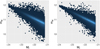 |
Fig. 1 Both plots: Relative frequencies of galaxies in the (Mr, mst)-plane are shown.The brighter the colour, the higher the frequency within a given pixel. The left plot is shown with all galaxies, whereas the right plot only shows galaxies with a neighbouring galaxy at a distance of r ∈ [1, 3] Mpc. The normalisation of the logarithmic quantities Mr and mst is given in Appendix A.1. |
3.1 Determining the range
To quantify the range of conformity, an exponential, a Lorentz function, and a power law are fitted2 to the observed scale dependent correlation coefficients as follows:
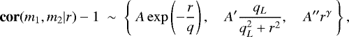 (8)
(8)
where q and qL are the scale parameters in the exponential and Lorentz model, and the power law is scale invariant. As can be seen from Fig. 2 in all six cases the exponential and the Lorentz fit perform similarly well, whereas the scale invariant power-law fit is significantly off. Quantitatively this can be seen from the summed residuals. For the exponential and Lorentz fit they are comparable in size, whereas for the power-law fit they are larger by an order of magnitude. The q and qL determined from fits range from 8 Mpc to 17 Mpc (see Table 2). This quantifies the visual expression from Fig. 2, which shows that the range of conformity depends on the galactic properties under investigation. An exponential or a Lorentz distribution function allows signals on scales larger than q and ql. Significant scale dependent correlation coefficients are seen up to 40 Mpc and beyond (cf. Fig. 2). The toy model in Appendix B further illustrates that a built-in scale in the correlation pattern of the mark distribution can be determined unambiguously with the scale dependent correlation coefficients cor (⋅, ⋅|r).
3.2 Alternative scale-dependent correlation coefficients
The results for the alternative definition of the scale dependent correlation coefficients  are shown in Fig. 2. The four combinations (Mr, e), (Mr, mst), (Mr, σv), and (mst, σv) show a reduced amplitude compared to cor(⋅, ⋅|r). With
  the scale dependent correlation coefficients is measured with respect to the mean and variance of the galaxies with another galaxy at a distance of r (see Eqs. (5) and (6)). With cor(⋅, ⋅|r) the correlations are calculated with respect to the mean and variance of all galaxies. It is well known that for galaxies the scale dependent mean
  and and variance
  are larger than the overall mean
  and variance
  for small distances r (see e.g. Beisbart & Kerscher 2000). Consequently a reduced amplitude should be expected from Eq. (7). Still the remaining signal traced by
  shows a similar long range of conformity outside the fluctuations. Also the combinations (e, mst) and (e, σv) show no significant deviation between
  and cor(⋅, ⋅|r), both confirming the long range of conformity.
3.3 Systematics
The results discussed in the preceding section were obtained from a volume limited galaxy sample from the SDSS DR12 with a limiting depth of 600 Mpc. Similar patterns can be observed for the scale dependent correlation coefficients from samples with 300 Mpc and 900 Mpc depth in Fig. 3. A more detailed look shows that the inclusion of less luminous galaxies in the 300 Mpc sample leads to a smaller amplitude of the scale dependent correlation coefficient and also a smaller estimate for the scale parameters, whereas an increased amplitude is observed forthe more luminous galaxies in the 900 Mpc sample. The amplitude and range of conformity is not universal, it depends on the galactic properties considered and on the luminosity cut used for the construction of the sample.
The absolute magnitude Mr is used as a mark but also used in the construction of the volume limited samples. Thus it is important to investigate how systematic changes in the calculation of Mr influence the results. The analysis was repeated for absolute magnitudes derived from the model magnitudes with no extinction correction (dereddening) and / or without employing a K-correction. As can be seen from Fig. 3, the results are very similar; only the results from samples with no extinction correction and no K-correction show a significantly enhanced amplitude and an even longer range of conformity. To check for a special kind of Malmquist bias (see Beisbart & Kerscher 2000, Sect. 4.5), the analysis was repeated for galaxies with a distance up to 580 Mpc, selected from the volume limited sample with limiting depth of 600 Mpc and no significant deviations were seen.
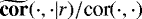
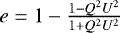
The ratios of luminosities in different filters are called colours. It is well known that colours are correlated with the morphological type and other properties of the galaxy, therefore colours should be natural candidates in the analysis presented above. However the scale dependent correlation coefficients for colours are sensitive to the extinction correction and K-correction. Differences on small scales and residual correlations on large scale can be seen for the colour Cur= Mu − Mr and the absolute magnitude Mr in Fig. 4. The amplitude of the scale dependent correlation coefficient between Mr, e, σv, and mst, obtained from samples with various magnitude estimates, differ slightly, but a consistent picture for the conformity on large scales appears. Consequently, the main results of this article, the long range of conformity, is not affected as can be seen from Figs. 2 and 3. Moreover, the sample using the extinction and K-corrected magnitudes gives the most conservativeestimates for the scale dependent correlation coefficients with the lowest amplitude and the smallest range of conformity. Unfortunately this is not the case for the scale dependent correlation coefficients of colour Cur and absolute magnitudes Mr (see Fig. 4). It is not clear whether the extinction correction, K-correction, or other currently unknown issues are responsible for these residuals and therefore colours are not considered any further in this work.
Instead of colours the spectral properties of the galaxies can be used directly. For example the velocity dispersion σv in galaxies are estimated from observed line widths. Also the stellar mass estimates rely heavily on spectral properties of the galaxies, and the stellar mass estimate can be regarded as a concise summary of the spectral properties of the galaxy. As briefly discussed in Appendix A.1 various methods employing a variety of spectral libraries can be used to estimate the stellar mass content mst. Repeating the analysis for the three different stellar mass estimates from the SDSS database leads to very similar results.
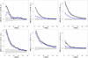 |
Fig. 2 Scale-dependent correlation functions cor(⋅, ⋅|r)∕cor(⋅, ⋅) of (Mr, e), (Mr, mst), (Mr, σv), (e, mst), (e, σv), and (mst, σv) calculated from the volume limited sample with 600 Mpc depth from the SDSS DR12 (thick solid line). The 1σ error bars around cor(⋅, ⋅|r) = cor(⋅, ⋅) are calculated from 50 galaxy samples with randomised marks. The exponential, Lorentz, and power-law fits, according to Eq. (8), are shown with a thin solid, dashed, and dotted line respectively. The thick blue dashed line shows the results for the alternative definition of the scale dependent correlation coefficients
|

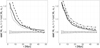 |
Fig. 3 Left plot: cor(Mr, σv | r)∕cor(Mr, σv) from volume limited samples with 300 Mpc depth (dotted), 600 Mpc depth (solid line), and 900 Mpc depth (dashed) are shown. Right plot: The results from the samples with various estimates of the absolute magnitude: K-corrected and extinction corrected (dereddened) model magnitudes (solid line), without extinction correction (dotted), without K-correction (dashed), without both, extinction correction and K-correction (dash-dotted). |
 |
Fig. 4 Value ofcor(Mr, Cur|r)∕cor(Mr, Cur) as calculatedfrom various estimates of the absolute magnitude Mr and colour Cur = Mu − Mr: K-corrected and extinction corrected magnitudes (solid line), without extinction correction (dotted), without K-correction (dashed), without both, extinction correction and K-correction (dash-dotted). |
4 Scale-dependent correlation coefficients of haloes from the MultiDark simulations
Dark matter simulations can be used to model the large scale distribution of matter in the universe. The dark matter concentrations in these simulations are called haloes. A direct comparison of the result for galaxies to the results from haloes is complicated by the fact that no luminous matter is included in the simulations. Still, analogous properties of the haloes can be used and the scale dependent correlation coefficients calculated from dark matter haloes can be qualitatively compared to the results from the galaxies. The focus is on the range of these scale dependent correlation coefficients. A related motivation for investigating halo catalogues comes from the observations in the galaxy catalogue that there are residuals in the scale dependent correlation coefficients for colours that are not well understood (see Sect. 3.3). The scale dependent correlation coefficients for the other galactic properties do not show these residuals but still one wishes for at least a qualitative cross check. Halo catalogues from dark matter simulations offer such clean well-defined samples without observational biases.
From the MultiDark simulations (MDPL2; Prada et al. 2012; Klypin et al. 2016) dark matter haloes are identified using the Rockstar halo finder (Behroozi et al. 2013). Haloes with a virial mass Mvir ≥ 1012M⊙ h−1 (thus with at least 662 dark matter particles per halo) are selected from the MDPL2 simulations. The Rockstar halo finder is able to determine sub-haloes within haloes. However in this analysis only distinct haloes, i.e. haloes that are not sub-haloes in any other halo are used. For a detailed description of how the substructure membership is determined see Behroozi et al. (2013), Sect. 3.4. The virial mass Mvir and dimensionless spin parameter λ of the haloes are used as marks and the ratio of the smallest axes to the largest axes in the mass ellipsoid (for details see Appendix A.2). No direct comparison of the scale dependent correlation coefficients from the dark matter haloes and the galaxy distribution is attempted, but analogous quantities are used as marks. For the dark matter haloes from the simulations the mass is directly accessible, whereas for galaxies the absolute magnitude and stellar mass content are biased tracers of the overall mass. The internal dynamical state is reflected in the spin of the halo and velocity dispersion of the galaxy. The shape of the halo is quantified from the 3D mass ellipsoid, and the shape of a galaxy from the 2D ellipticity obtained from the image of the galaxy.
The correlation coefficients between Mvir, λ, and s in the halo sample are summarized in Table 3. Such correlations are expected. For a detailed study of these one point correlations see for example Knebe & Power (2008) and Vega-Ferrero et al. (2017). The corresponding scale dependent correlation coefficients are shown in Fig. 5. The overall appearance is similar to the scale dependent correlation coefficients observed in the galaxy distribution (Fig. 2) with some exceptions. The amplitude of the scale dependent correlation coefficients on small scales is stronger for the combinations (Mvir, λ), and (Mvir, s) compared toany of the results from the galaxy distribution. Also, the range of conformity is larger for the haloes compared to the galaxies; seealso the fitted scale parameters of the halo sample in Table 4 compared to the scale parameters of the galaxy sample in Table 2. Similar to the galaxy distribution, the alternative scale dependent correlation coefficients  show a reduced amplitude. Still (λ, s) shows long range correlations out to 30 Mpc, but the signal in (Mvir, λ) and (Mvir, s) is confined to scales below 10 and 15 Mpc.
Correlation coefficients between Mvir, λ, and s determined from the MDPL2 Rockstar halo sample with Mvir ≥ 1012M⊙ h−1.
Systematics
To investigate the dependence on the mass cut, samples with Mvir ≥ 5 × 10¹¹M⊙ h−1, Mvir ≥ 1 × 10¹²M⊙ h−1, and Mvir ≥ 1013M⊙ h−1 have been analysed. The scale dependent correlation coefficients show a similar shape and in most cases a similar amplitude between the halo sample. As can be seen in Fig. 6 the amplitude and range of conformity increases in the two samples with the mass cut from Mvir ≥ 5 × 10¹¹M⊙ h−1 to Mvir ≥ 1 × 10¹²M⊙ h−1. A similar behaviour can be observed in the galaxy samples including more luminous galaxies (see Fig. 3). The most massive sample with Mvir ≥ 1 × 10¹³M⊙ h−1 shows a dip in the scale dependent correlation coefficient on scales below 5 Mpc, but very similar results compared to the sample with Mvir ≥ 1 × 10¹²M⊙ h−1 on a large scale. Also the scale-dependent correlation coefficients of halo samples from the BigMDPL simulations (box size 2.5 Gpc h−1) show a similar long range of conformity.
The Rockstar halo finder is able to determine a halo hierarchy. In the analysis for Fig. 5 only distinct haloes, i.e. haloes that are not marked as a sub-haloes, are used. The scale dependent correlation coefficients calculated from all the haloes, including sub-haloes and their parent haloes, show a reduced amplitude as can be seen in Fig. 6. The Rockstar halo finder uses phase-space information and an elaborate unbinding strategy to define the halos. The 3D friend-of-friend (FoF) halo finder operates only in position space to identify halos as linked particle over-densities (Riebe et al. 2013). The analysis with the scale dependent correlation coefficients is repeated forsuch FoF halo samples from the same MDPL2 simulation. Again the mass, spin, and axis ratios of the ellipsoidal shape are used as marks (see Riebe et al. 2013 for details). By comparing the corresponding scale dependent correlation coefficient of Rockstar and FoF halo samples, an increased amplitude can be seen in Fig. 6. Although the amplitude of the scale dependent correlation coefficients differ between all haloes, distinct haloes, and FoF-haloes, the signal of a long range of conformity is clearly visible in all the samples.
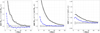 |
Fig. 5 Scale-dependent correlation functions of (Mvir, λ), (Mvir, s), and (λ, s), calculated from the MDPL2 Rockstar halo sample with Mvir ≥ 1012M⊙ h−1 (thick solid line). The 1σ error bars around cor(⋅, ⋅|r) = cor(⋅, ⋅) are calculated from 50 halo samples with randomised marks. The exponential, Lorentz, and power-law fits, according to Eq. (8), are shown with thin solid, dashed, and dotted lines, respectively. |
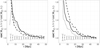 |
Fig. 6 Left plot: cor(Mvir, λ | r)∕cor(Mvir, λ) are shown for samples with a mass cut Mvir ≥ 5 × 10¹¹M⊙ h−1 (dashed), Mvir ≥ 1 × 10¹²M⊙ h−1 (solid line), and Mvir ≥ 1013M⊙ h−1 (dotted). Right plot: the results from samples using various halo identification methods are shown: Rockstar distinct haloes (solid line), Rockstar all haloes (dotted), and FoF haloes (dashed). |
5 Summary and outlook
Properties of galaxies show scale dependent correlation coefficients out to large scales. Properties such as mass and luminosity are significantly stronger (anti-) correlated for close pairs compared to the correlation coefficients in the overall sample. This is a clear signal of conformity. The analysis was carried out with a new descriptive statistic – the scale dependent correlation coefficients. These quantify how the correlation coefficients between galactic properties vary under the condition that another galaxy (or halo) is at a distance of r. This signal of galactic conformity extends to large scales, and in several cases become consistent with mark independent clustering only beyond40 Mpc. Several tests for systematic effects confirm the long range of conformity. Halo samples from dark matter simulations show a larger amplitude and an even longer range of conformity. The scale dependent correlation coefficients between for example mass and shape clearly deviates from the overall correlation coefficient beyond 40 Mpc. No universal range of conformity is found. The range varies for various properties under investigation and also depends on the luminosity and mass cut used in the construction of the samples. Such a long range of conformity goes well with the investigations of Faltenbacher et al. (2002), who found alignment correlations for cluster sized haloes out to separations of 100 Mpc h−1. The focus ofthe present investigation was on the introduction of the scale dependent correlation coefficients and on the detection of a long range of conformity. On small scales more complicated patterns are expected and further investigations of the scale dependent conformity should be accompanied by a detailed modelling.
Pure dark matter simulations capture only the gravitational part but allow for a large number of haloes and convincing statistics. As shown by Gottlöber & Yepes (2007) and Teklu et al. (2015) there exists a complex interplay between the spin, mass, and morphology of the dark matter and the gas component within haloes. It will be highly interesting to investigate the environmental dependence of such haloes using the scale dependent correlation coefficients.
Empirical relations, such as the Tully-Fisher or the fundamental plane relation are special correlations between the properties of a galaxy (see e.g. Kelson et al. 2000; Saulder et al. 2013 and references therein). These empirical relations, such as the fundamental plane, depend on the amount of substructure in the objects (see Fritsch & Buchert. 1999 for galaxy clusters). Hence one can expect that an extended version of the scale dependent correlation coefficients could be used to investigate the spatial scale dependence of such empirical relations.
As already mentioned, a detailed modelling of this signal of conformity is the next step. Purely geometric models, such as the toy model in Appendix B help us to appreciate the method, but often do not promote a physical understanding. Consquently more physically motivated models are clearly needed.
Inspired by the ideas of hierarchical structure formation in dark matter models, the halo model was designed to explain the clustering of galaxies (see Cooray & Sheth 2002 for a review). The halo model is able to reproduce the signal from the mark weighted correlation function out to 20 Mpc (Skibba et al. 2006, see also Paranjape et al. 2015 and Pahwa & Paranjape 2017 for a more detailed model of galactic conformity). Within these models the contribution from the so-called two-halo term seems necessary to explain conformity on large scales. A physical explanation of galactic conformity from structure formation was given by Hearin et al. (2016), who called this assembly bias. Their explanation is elaborated for pair distances below 10 Mpc, but possibly their arguments could be extended to large scales as well.
Another approach is based on the peak theory (Bardeen et al. 1986). Recently Verde et al. (2014) calculated the Lagrangian (formation) bias for a Gaussian density field. The matter density field can be approximated more reliable using a logarithmic transformation (Falck et al. 2012) which could serve as an improved starting point for such a bias calculation. Closely related to the log-normal density field, the log-normal model for the galaxy distribution (Coles & Jones 1991; Møller et al. 1998) can be used as a stochastic model for the point and mark distribution. For such an intensity marked point process, the mark correlation functions can be calculated explicitly (Ho & Stoyan 2008; Myllymäki & Penttinen 2009). The adaption to the galaxy distribution reveals whether a natural parametrisation is possible within this model.
Acknowledgements
I would like to thank Stefan Gottlöber for the hospitality and discussions at the AIP. I am grateful to Kristin Riebe and Ben Hoyle for support and information on using the CosmoSim and the SDSS database, respectively. Special thanks to Claus Beisbart and Alex Szalay, some of the ideas for this analysis emerged from discussions now more than ten years ago. For comments on the manuscript I would like to thank Thomas Buchert, Stefan Gottlöber, and Volker Müller. I appreciate very much comments by Simon White, who suggested the alternative definition of the scale dependent correlation coefficient in Eq. (7) to me. I would like to thank the anonymous referee for his constructive and helpful comments. Funding for SDSS-III has been provided by the Alfred P. Sloan Foundation, the Participating Institutions, the National Science Foundation, and the U.S. Department of Energy Office of Science. The SDSS-III website is http://www.sdss3.org/. SDSS-III is managed by the Astrophysical Research Consortium for the Participating Institutions of the SDSS-III Collaboration including the University of Arizona, the Brazilian Participation Group, Brookhaven National Laboratory, Carnegie Mellon University, University of Florida, the French Participation Group, the German Participation Group, Harvard University, the Instituto de Astrofisica de Canarias, the Michigan State/Notre Dame/JINA Participation Group, Johns Hopkins University, Lawrence Berkeley National Laboratory, Max Planck Institute for Astrophysics, Max Planck Institute for Extraterrestrial Physics, New Mexico State University, New York University, Ohio State University, Pennsylvania State University, University of Portsmouth, Princeton University, the Spanish Participation Group, University of Tokyo, University of Utah, Vanderbilt University, University of Virginia, University of Washington, and Yale University. This research made use of the “K-corrections calculator” service, especially the python code, available at http://kcor.sai.msu.ru/. The CosmoSim database used in this paper is a service by the Leibniz-Institute for Astrophysics Potsdam (AIP). The MultiDark database was developed in cooperation with the Spanish MultiDark Consolider Project CSD2009-00064. The Bolshoi and MultiDark simulations have been performed within the Bolshoi project of the University of California High-Performance AstroComputing Center (UC-HiPACC) and were run at the NASA Ames Research Center. The Multidark Planck (MDPL) and the BigMD simulation suite have been performed in the Supermuc supercomputer at LRZ using time granted by PRACE. In the numerical analysis Python with scipy and for the plotting R with ggplot2 have been used (Jones et al. 2017; R Core Team 2015; Wickham 2009).
Appendix A Samples
A.1 Galaxay catalogues from the SDSS III, DR12
In the SDSS DR12 data release (Alam et al. 2015; Eisenstein et al. 2011) each galaxy comes with a wealth of properties. The galaxy samples for the analysis are built in two stages. First, a basic galaxy sample is obtained from the SDSS database, then derived quantities are calculated and the volume limited samples are constructed. Our basic galaxy sample was extracted from the SDSS database, as provided via CasJobs3, using the SQL script shown in Table A.1. The query starts with the view SpecPhoto and joins it with Galaxy and SpecObj to gain access to further photometric and spectroscopic parameters. The joins with the tables stellarMassPCAWiscM11/ PCAWiscBC03/stellarMassStarformingPort are used to obtain the stellar mass estimates. In the joins with the stellar mass tables some galaxies could not be matched and 0.11% of the galaxies are lost. The function fCosmoDl provided in the SDSS database is used to calculate the luminosity distance from the redshift, using a Planck-like cosmology consistent with the MultiDark simulations; see Appendix A.2. The selection in the where clause is mostly the original selection as used for the SDSS main galaxy sample (Strauss et al. 2002). From this basic sample the following parameters are calculated for each galaxy.
The SQL code used on CasJobs to extract the basic sample from SDSS DR12.
-
Absolute magnitudes:
The absolute magnitude Mr in the r band is calculated from the extinction corrected (dereddened) model magnitude mr using Mr = mr − D, with the distance module D = 5log10(d∕10pc) and the luminosity distance d in pc. The absolute magnitude is K-corrected using thepython code from http://kcor.sai.msu.ru/, version 2012, implementing the methods described in Chilingarian et al. (2010) and Chilingarian & Zolotukhin (2012). See also the comparison of several K-corrections in O’Mill et al. (2011)
-
Ellipticities:
The ellipticities e of the galaxies are calculated from the Stokes parameters Q and U using
 . The Stokes parameters Q
and U
have been estimated from the intensity profile of the galaxies in the r
band using the adaptive moments mE1r
and mE2r
respectively (Bernstein & Jarvis 2002). This ellipticity e
is an estimate of the observed 2D ellipticity on the sky. No attempt is made to derive a 3D/de-projected ellipticity.
. The Stokes parameters Q
and U
have been estimated from the intensity profile of the galaxies in the r
band using the adaptive moments mE1r
and mE2r
respectively (Bernstein & Jarvis 2002). This ellipticity e
is an estimate of the observed 2D ellipticity on the sky. No attempt is made to derive a 3D/de-projected ellipticity. -
Stellar mass content:
Using the photometry and the spectra the stellar mass content of a galaxy can be estimated. The following three mass estimates can be retrieved from the SDSS database. They use various stellar population synthesis models and various methods: The table stellarMassPCAWiscM11 provides stellar mass estimates using the method of Chen et al. (2012) with the stellar population synthesis models of Maraston & Strömbäck (2011). These are the stellar mass estimates used for the plots in Fig. 2. The table stellarMassPCAWiscBC03 provides stellar mass estimates using the method of Chen et al. (2012) with the stellar population synthesis models of Bruzual & Charlot (2003), and the table stellarMassStarformingPort provides stellar mass estimates using the method of Maraston et al. (2006); see also Maraston et al. (2013).
Irrespective of the method, mst = logMst∕M⊙ is used as a mark in the analysis, Mst is the stellar mass content, and M⊙ the solar mass. Both mst and the magnitude Mr are logarithmic in mass and luminosity, respectively.
-
Velocity dispersion:
The velocity dispersion σv inside the galaxy is estimated from the spectra as described in Bolton et al. (2012) and is directly read from the database view SpecObj.
The volume limited samples comprise galaxies with luminosity distance d ≤ dlim. and absolute magnitude Mr ≤ Mlim.. The limiting absolute magnitude is Mlim. = mlim. − Dlim. with the (conservative) limiting magnitude mlim. = 17.7 and the limiting distance module Dlim. = 5log10(dlim.∕10pc); also galaxies close by with luminosity distance d ≤ 50 Mpc are discarded. Mainly, the volume limited sample with dlim. = 600 Mpc and 201722 galaxies is used, but also samples with dlim. = 300 Mpc and 900 Mpc are considered.
SQL code used on CosmoSim to extract Rockstar haloes with Mvir ≥ 1012M⊙ h−1 at z = 0 from the MDPL2 simulation.
A.2 Halo samples from MultiDark simulations
The halo catalogues are constructed from the so-called MultiDark simulations, which are dark matter simulations as described in Prada et al. (2012) and Klypin et al. (2016). The MDPL2 and BigMDPL simulations have a box size of 1 Gpc/h and 2.5 Gpc/h, respectively, and have Planck-like cosmology Ω m = 0.307115, Ω Λ = 0.692885, Ω rad = 0.0, Ω 0 = −1.0, h = 0.6777. The dark matter haloes were identified using the Rockstar halo finder (Behroozi et al. 2013). These halo samples can be downloaded from the CosmoSim database4 as describedin Riebe et al. (2013).
Figure A.2 shows the SQL code used to extract one of the desired halo samples from the CosmoSim database. About 4 × 10⁶ distinct haloes with a virial mass Mvir ≥ 1012M⊙∕h are selected. With snapnum=125 we select the z = 0 samples and with pId=-1 we ask for distinct haloes only. The virial mass Mvir, the spin λ, and the shape s are used as marks (see below). They can be accessed directly from the database. To facilitate the calculations of the scale dependent correlation functions a random subsample comprising 25% of the haloes is used (about 106 haloes). A comparison with the results from 10% and 50% subsampling shows that the results for the scale dependent correlation coefficients clearly stabilise for 25% subsampling.
-
Mass:
The mass Mvir within the virial radius is calculated from the number of bound particles in the halo. The major task of this phase-space halo finder is to reliably assign the dark matter particles to a halo, using several steps as detailed in Behroozi et al. (2013).
-
Spin:
The dimensionless spin parameter λ is used to quantify the rotation of galactic systems (see e.g. Fall & Efstathiou 1980).
-
Shape:
The axial ratios of the mass ellipsoid are determined according to the method of Allgood et al. (2006) using the eigenvalues of the (reduced) inertia tensor of the halo. The ratio of the smallest ellipsoid axes to the largest ellipsoid axes is then used as an overall shape parameter s.
To investigate systematic effects halo samples with mass cuts Mvir ≥ 5 × 10¹¹M⊙ h−1 and Mvir ≥ 1013M⊙ h−1 have also been extracted from the MDPL2 and BigMDPL simulations. Also the mass, spin, and axis ratios of the ellipsoidal shape determined from FoF haloes have been used (see Riebe et al. 2013 and https://www.cosmosim.org/ for details).
Appendix B A toy model
The following model is a straightforward extension of the marked Poisson process discussed by Wälder & Stoyan (1996). This model serves as an illustration that it is possible to unambiguously extract a scale from a marked point distribution using the scale dependent correlation coefficient cor(m1, m2 | r). It is not meant to be a viable model for the galaxy distribution.
Beginning with a Poisson process, i.e. randomly distributed points with number density ϱ. As suggested by Wälder & Stoyan (1996) the number of other points within a radius R is assigned to each point as a mark m1. This mark m1 is a Poisson random variable with the mean mark ![Mathematical equation: $E[m_1]=\overline{m}=\varrho\frac{4\pi}{3}R^3$](/articles/aa/full_html/2018/07/aa31212-17/aa31212-17-eq54.png) and the variance
and the variance  . Therefore the probability of observing n points in a sphere with radius R is
 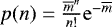 .
.
As an extension of this model, the second mark on a point is slaved to its first mark by m2 = m1. This construction leads to the covariance  and perfect overall correlation cor(m1, m2) = 1. For the Poisson point process, it is easy to calculate the desired scale dependent correlation coefficients. The point x is marked with m2 = m1 as described above. If a second point at y is more distant than |x −y| = r > R, the number of points inside the sphere around point x is independentfrom the point at y and cov(m1, m2 | r) = cov(m1, m2). Under the condition that the second point at y is closer than R, at least one point is always in the sphere around the point at x. Considering a Poisson point process, all the other points are still independent from this point at y. Now the probability q(l) of observing l points in the sphere around x is q(0) = 0 and q(l) = p(l − 1). This allows us to calculate
![Mathematical equation: \begin{align*} \textbf{cov}(m_1,m_2\,|\,r) & = E_q[(m_1-\overline{m})(m_2-\overline{m})] \\ & = E_q\left[(m_1-\overline{m})^2\right] =\overline{m}+1, \end{align*}](/articles/aa/full_html/2018/07/aa31212-17/aa31212-17-eq58.png)
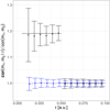 |
Fig. B.1 Value of cor(m1, m2 | r)∕cor(m1, m2) estimated from 100 realisations of a marked Poisson process with R = 0.05 and ϱ = 10 000 in the unit box (points with 1σ error bars). The solid line is the theoretical curve according to Eq. (B.1). The blue dashed curve shows the results for |

for r ≤ R. Eq is the expectation with respect to the probabilites q(l). Joining the results from above one obtains
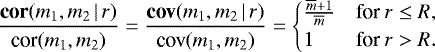 (B.1)
(B.1)
A similar reasoning allows the calculation of  . If the second point at y is farther away than R, we get
  and
and  and therefore
  . If the second point is closer than R, one obtains
 ![Mathematical equation: $\overline{m}(r)=E_q[m_1]$](/articles/aa/full_html/2018/07/aa31212-17/aa31212-17-eq64.png) and
and ![Mathematical equation: $\sigma_m^2(r)=E_q[(m_1-\overline{m}(r))^2]$](/articles/aa/full_html/2018/07/aa31212-17/aa31212-17-eq65.png) , and
, and
![Mathematical equation: \begin{align*} \widetilde{\textbf{cov}}(m_1,m_2\,|\,r) & = E_q[(m_1-\overline{m}(r))(m_2-\overline{m}(r))]\\ & = E_q\left[(m_1-\overline{m}(r))^2\right] = \sigma_m^2(r). \end{align*}](/articles/aa/full_html/2018/07/aa31212-17/aa31212-17-eq66.png)
Putting everything together  for all radii r. The scale R cannot be resolved with
  .
.
In Fig. B.1 the estimated cor(m1, m2 | r) for the marked Poisson process is compared to the theoretical expectation showing perfect agreement. The jump in cor (m1, m2 | r) is resolved, marking the built-in scale. As it should be  is approximately 1 on all scales. This simple model illustrates that a built–in scale in the correlation pattern of the marks can be resolved unambiguously with cor(m1, m2 | r), whereas the alternative definition
  does not allow this.
References
- Alam, S., Albareti, F. D., Allende Prieto, C., et al. 2015, ApJS, 219, 12 [NASA ADS] [CrossRef] [Google Scholar]
- Allgood, B., Flores, R. A., Primack, J. R., et al. 2006, MNRAS, 367, 1781 [NASA ADS] [CrossRef] [Google Scholar]
- Andreon, S., Davoust, E., & Heim, T. 1997, A&A, 323, 337 [NASA ADS] [Google Scholar]
- Bardeen, J. M., Bond, J. R., Kaiser, N., & Szalay, A. S. 1986, ApJ, 304, 15 [NASA ADS] [CrossRef] [Google Scholar]
- Behroozi, P. S., Wechsler, R. H., & Wu, H.-Y. 2013, ApJ, 762, 109 [NASA ADS] [CrossRef] [Google Scholar]
- Beisbart, C., & Kerscher, M. 2000, ApJ, 545, 6 [NASA ADS] [CrossRef] [Google Scholar]
- Beisbart, C., Kerscher, M., & Mecke, K. 2002, in Morphology of Condensed Matter Physics and Geometry of Spatially Complex Systems, ed. K. R. Mecke, & D. Stoyan, Lect. Notes Phys. No. 600 (Berlin: Springer Verlag), 358 [Google Scholar]
- Bernstein, G. M., & Jarvis, PM. 2002, AJ, 123, 583 [NASA ADS] [CrossRef] [Google Scholar]
- Binggeli, B., Tarnghi, M., & Sandage, A. 1990, A&A, 1228, 42 [NASA ADS] [Google Scholar]
- Bolton, A. S., Schlegel, D. J., Aubourg, É., et al. 2012, AJ, 144, 144 [NASA ADS] [CrossRef] [Google Scholar]
- Bruzual, G., & Charlot, S. 2003, MNRAS, 344, 1000 [NASA ADS] [CrossRef] [Google Scholar]
- Chen, Y.-M., Kauffmann, G., Tremonti, C. A., et al. 2012, MNRAS, 421, 314 [NASA ADS] [Google Scholar]
- Chilingarian, I. V., & Zolotukhin, I. Y. 2012, MNRAS, 419, 1727 [NASA ADS] [CrossRef] [Google Scholar]
- Chilingarian, I. V., Melchior, A.-L., & Zolotukhin, I. Y. 2010, MNRAS, 405, 1409 [NASA ADS] [CrossRef] [Google Scholar]
- Coles, P., & Jones, B. 1991, MNRAS, 248, 1 [NASA ADS] [CrossRef] [Google Scholar]
- Cooray, A., & Sheth, R. 2002, Phys. Rep., 372, 1 [NASA ADS] [CrossRef] [Google Scholar]
- Desjacques, V., Jeong, D., & Schmidt, F. 2016, Phys. Rep., 733, 1 [Google Scholar]
- Dressler, A. 1980, ApJ, 236, 351 [NASA ADS] [CrossRef] [Google Scholar]
- Eisenstein, D. J., Weinberg, D. H., Agol, E., et al. 2011, AJ, 142, 72 [Google Scholar]
- Falck, B. L., Neyrinck, M. C., Aragon-Calvo, M. A., Lavaux, G., & Szalay, A. S. 2012, ApJ, 745, 17 [NASA ADS] [CrossRef] [Google Scholar]
- Fall, S. M., & Efstathiou, G. 1980, MNRAS, 193, 189 [NASA ADS] [CrossRef] [Google Scholar]
- Faltenbacher, A., Kerscher, M., Gottlöber, S., & Mueller, V. 2002, A&A, 395, 1 [NASA ADS] [CrossRef] [EDP Sciences] [Google Scholar]
- Fritsch, C., & Buchert., T. 1999, A&A, 344, 749 [NASA ADS] [Google Scholar]
- Gottlöber, S., & Yepes, G. 2007, ApJ, 664, 117 [NASA ADS] [CrossRef] [Google Scholar]
- Gottlöber, S., Kerscher, M., Kravtsov, A. V., et al. 2002, A&A, 387, 778 [NASA ADS] [CrossRef] [EDP Sciences] [Google Scholar]
- Grabarnik, P., Myllymäki, M., & Stoyan, D. 2011, Ecol. Model., 23, 3888 [CrossRef] [Google Scholar]
- Hamilton, A. J. S. 1988, ApJ, 331, L59 [NASA ADS] [CrossRef] [Google Scholar]
- Hearin, A. P., Watson, D. F., & van den Bosch, F. C. 2015, MNRAS, 452, 1958 [NASA ADS] [CrossRef] [Google Scholar]
- Hearin, A. P., Behroozi, P. S., & van den Bosch, F. C. 2016, MNRAS, 461, 2135 [NASA ADS] [CrossRef] [Google Scholar]
- Ho, L. P., & Stoyan, D. 2008, Stat. Probab. Lett., 78, 1194 [CrossRef] [Google Scholar]
- Jones, E., Oliphant, T., Peterson, P., et al. 2017, SciPy: Open Source scientific Tools for Python [Online; accessed April 22, 2017] [Google Scholar]
- Kaiser, N. 1984, ApJ, 284, L9 [NASA ADS] [CrossRef] [Google Scholar]
- Kauffmann, G., Li, C., Zhang, W., & Weinmann, S. 2013, MNRAS, 430, 1447 [NASA ADS] [CrossRef] [Google Scholar]
- Kelson, D. D., Illingworth, G. D., Tonry, J. L., et al. 2000, ApJ, 529, 768 [NASA ADS] [CrossRef] [Google Scholar]
- Klypin, A., Yepes, G., Gottlöber, S., Prada, F., & Heß, S. 2016, MNRAS, 457, 4340 [NASA ADS] [CrossRef] [Google Scholar]
- Knebe, A., & Power, C. 2008, ApJ, 678, 621 [NASA ADS] [CrossRef] [Google Scholar]
- Lacerna, I., Contreras, S., González, R. E., Padilla, N., & Gonzalez-Perez, V. 2018, MNRAS, 475, 1177 [NASA ADS] [CrossRef] [Google Scholar]
- Maraston, C., & Strömbäck, G. 2011, MNRAS, 418, 2785 [NASA ADS] [CrossRef] [Google Scholar]
- Maraston, C., Daddi, E., Renzini, A., et al. 2006, ApJ, 652, 85 [NASA ADS] [CrossRef] [Google Scholar]
- Maraston, C., Pforr, J., Henriques, B. M., et al. 2013, MNRAS, 435, 2764 [NASA ADS] [CrossRef] [Google Scholar]
- Møller, J., Syversveen, A. R., & Waagepetersen, R. P. 1998, Scand. J. Stat., 25, 451 [CrossRef] [Google Scholar]
- Myllymäki, M., & Penttinen, A. 2009, Stat. Neerl., 63, 450 [CrossRef] [Google Scholar]
- O’Mill, A. L., Duplancic, F., García Lambas, D., & Sodré, Jr. L. 2011, MNRAS, 413, 1395 [NASA ADS] [CrossRef] [Google Scholar]
- Ostriker, J. P., & Turner, E. L. 1979, ApJ, 234, 785 [NASA ADS] [CrossRef] [Google Scholar]
- Pahwa, I., & Paranjape, A. 2017, MNRAS, 470, 1298 [NASA ADS] [CrossRef] [Google Scholar]
- Paranjape, A., Kovač, K., Hartley, W. G., & Pahwa, I. 2015, MNRAS, 454, 3030 [NASA ADS] [CrossRef] [Google Scholar]
- Postman, M., & Geller, M. 1984, ApJ, 281, 95 [NASA ADS] [CrossRef] [Google Scholar]
- Prada, F., Klypin, A. A., Cuesta, A. J., Betancort-Rijo, J. E., & Primack, J. 2012, MNRAS, 423, 3018 [NASA ADS] [CrossRef] [Google Scholar]
- R Core Team 2015, R: A Language and Environment for Statistical Computing, R Foundation for Statistical Computing, Vienna, Austria [Google Scholar]
- Riebe, K., Partl, A. M., Enke, H., et al. 2013, Astron. Nachr., 334, 691 [NASA ADS] [CrossRef] [EDP Sciences] [Google Scholar]
- Saulder, C., Mieske, S., Zeilinger, W. W., & Chilingarian, I. 2013, A&A, 557, A21 [NASA ADS] [CrossRef] [EDP Sciences] [Google Scholar]
- Sheth, R. K., & Tormen, G. 2004, MNRAS, 350, 1385 [NASA ADS] [CrossRef] [EDP Sciences] [Google Scholar]
- Skibba, R., Sheth, R. K., Connolly, A. J., & Scranton, R. 2006, MNRAS, 369, 68 [NASA ADS] [CrossRef] [Google Scholar]
- Stoyan, D. 1984, Math. Nachr., 116, 197 [CrossRef] [Google Scholar]
- Stoyan, D., & Stoyan, H. 1994, Fractals, Random Shapes and Point Fields (Chichester: John Wiley & Sons) [Google Scholar]
- Strauss, M. A., Weinberg, D. H., Lupton, R. H., et al. 2002, AJ, 124, 1810 [NASA ADS] [CrossRef] [Google Scholar]
- Szapudi, I., Branchini, E., Frenk, C., Maddox, S., & Saunders, W. 2000, MNRAS, 319, L45 [NASA ADS] [CrossRef] [Google Scholar]
- Teklu, A. F., Remus, R.-S., Dolag, K., et al. 2015, ApJ, 812, 29 [Google Scholar]
- van der Wel, A., Bell, E. F., Holden, B. P., Skibba, R. A., & Rix, H.-W. 2010, ApJ, 714, 1779 [NASA ADS] [CrossRef] [Google Scholar]
- Vega-Ferrero, J., Yepes, G., & Gottlöber, S. 2017, MNRAS, 467, 3226 [Google Scholar]
- Verde, L., Jimenez, R., Simpson, F., et al. 2014, MNRAS, 443, 122 [NASA ADS] [CrossRef] [Google Scholar]
- Wälder, O., & Stoyan, D. 1996, Biom. J., 38, 895 [CrossRef] [Google Scholar]
- Weinmann, S. M., van den Bosch, F. C., Yang, X., & Mo, H. J. 2006, MNRAS, 366, 2 [NASA ADS] [CrossRef] [Google Scholar]
- Wickham, H. 2009, Ggplot2: Elegant Graphics for Data Analysis (New York: Springer-Verlag) [Google Scholar]
- Willmer, C., da Costa, L. N., & Pellegrini, P. 1998, AJ, 115, 869 [NASA ADS] [CrossRef] [Google Scholar]
- Zehavi, I., Zheng, Z., Weinberg, D. H., et al. 2011, ApJ, 736, 59 [NASA ADS] [CrossRef] [Google Scholar]
This alternative definition of  was suggested to me by Simon White after the first submission of this article.
The weighted least-squares fit is performed with the function nls from the statistic package R using the inverse variance of the randomised sample as weights.
All Tables
Correlation coefficients between Mvir, λ, and s determined from the MDPL2 Rockstar halo sample with Mvir ≥ 1012M⊙ h−1.
SQL code used on CosmoSim to extract Rockstar haloes with Mvir ≥ 1012M⊙ h−1 at z = 0 from the MDPL2 simulation.
All Figures
|
Fig. 1 Both plots: Relative frequencies of galaxies in the (Mr, mst)-plane are shown.The brighter the colour, the higher the frequency within a given pixel. The left plot is shown with all galaxies, whereas the right plot only shows galaxies with a neighbouring galaxy at a distance of r ∈ [1, 3] Mpc. The normalisation of the logarithmic quantities Mr and mst is given in Appendix A.1. |
| In the text | |
|
Fig. 2 Scale-dependent correlation functions cor(⋅, ⋅|r)∕cor(⋅, ⋅) of (Mr, e), (Mr, mst), (Mr, σv), (e, mst), (e, σv), and (mst, σv) calculated from the volume limited sample with 600 Mpc depth from the SDSS DR12 (thick solid line). The 1σ error bars around cor(⋅, ⋅|r) = cor(⋅, ⋅) are calculated from 50 galaxy samples with randomised marks. The exponential, Lorentz, and power-law fits, according to Eq. (8), are shown with a thin solid, dashed, and dotted line respectively. The thick blue dashed line shows the results for the alternative definition of the scale dependent correlation coefficients
|
| In the text | |
|
Fig. 3 Left plot: cor(Mr, σv | r)∕cor(Mr, σv) from volume limited samples with 300 Mpc depth (dotted), 600 Mpc depth (solid line), and 900 Mpc depth (dashed) are shown. Right plot: The results from the samples with various estimates of the absolute magnitude: K-corrected and extinction corrected (dereddened) model magnitudes (solid line), without extinction correction (dotted), without K-correction (dashed), without both, extinction correction and K-correction (dash-dotted). |
| In the text | |
|
Fig. 4 Value ofcor(Mr, Cur|r)∕cor(Mr, Cur) as calculatedfrom various estimates of the absolute magnitude Mr and colour Cur = Mu − Mr: K-corrected and extinction corrected magnitudes (solid line), without extinction correction (dotted), without K-correction (dashed), without both, extinction correction and K-correction (dash-dotted). |
| In the text | |
|
Fig. 5 Scale-dependent correlation functions of (Mvir, λ), (Mvir, s), and (λ, s), calculated from the MDPL2 Rockstar halo sample with Mvir ≥ 1012M⊙ h−1 (thick solid line). The 1σ error bars around cor(⋅, ⋅|r) = cor(⋅, ⋅) are calculated from 50 halo samples with randomised marks. The exponential, Lorentz, and power-law fits, according to Eq. (8), are shown with thin solid, dashed, and dotted lines, respectively. |
| In the text | |
|
Fig. 6 Left plot: cor(Mvir, λ | r)∕cor(Mvir, λ) are shown for samples with a mass cut Mvir ≥ 5 × 10¹¹M⊙ h−1 (dashed), Mvir ≥ 1 × 10¹²M⊙ h−1 (solid line), and Mvir ≥ 1013M⊙ h−1 (dotted). Right plot: the results from samples using various halo identification methods are shown: Rockstar distinct haloes (solid line), Rockstar all haloes (dotted), and FoF haloes (dashed). |
| In the text | |
|
Fig. B.1 Value of cor(m1, m2 | r)∕cor(m1, m2) estimated from 100 realisations of a marked Poisson process with R = 0.05 and ϱ = 10 000 in the unit box (points with 1σ error bars). The solid line is the theoretical curve according to Eq. (B.1). The blue dashed curve shows the results for |
| In the text | |
Current usage metrics show cumulative count of Article Views (full-text article views including HTML views, PDF and ePub downloads, according to the available data) and Abstracts Views on Vision4Press platform.
Data correspond to usage on the plateform after 2015. The current usage metrics is available 48-96 hours after online publication and is updated daily on week days.
Initial download of the metrics may take a while.