| Issue |
A&A
Volume 614, June 2018
|
|
|---|---|---|
| Article Number | L4 | |
| Number of page(s) | 6 | |
| Section | Letters to the Editor | |
| DOI | https://doi.org/10.1051/0004-6361/201833181 | |
| Published online | 27 June 2018 | |
Letters to the Editor
Are all RR Lyrae stars modulated?
Konkoly Observatory of the Hungarian Academy of Sciences, Budapest 1121, Konkoly Thege ut. 13–15, Hungary
e-mail: This email address is being protected from spambots. You need JavaScript enabled to view it.
Received:
6
April
2018
Accepted:
25
May
2018
Abstract
We analyzed 151 variables previously classified as fundamental mode RR Lyrae stars from Campaigns 01–04 of the Kepler two-wheel (K2) archive. By employing a method based on the application of systematics filtering with the aid of co-trending light curves in the presence of a large amplitude signal component, we searched for additional Fourier signals in the close neighborhood of the fundamental period. We found only 13 stars without such components, yielding the highest rate of modulated (Blazhko) stars detected so far (91 %). A detection efficiency test suggests that this occurrence rate likely implies a 100 % underlying rate. Furthermore, the same test performed on a subset of the Large Magellanic Cloud RR Lyrae stars from the MACHO archive shows that the conjecture of high true occurrence rate fits well to the low observed rate derived from this database.
Key words: methods: data analysis / stars: variables: RR Lyrae
© ESO 2018
1. Introduction
RR Lyrae stars are among the most important objects for tracing galaxy structure and chemistry. They are thought to pulsate mainly in the radial modes, allowing nonlinear modeling of their basic properties from as early as the mid sixties (Christy 1964). Nevertheless, it is highly disturbing that modelling other than simple periodic pulsations (e.g., steady multimode states), our current (admittedly simple) models fail in a major way. This is particularly the case when considering stars with (quasi)periodic amplitude/phase change, commonly known as the Blazhko phenomenon (Blazhko 1907, see also Shapley 1916). Most of the progress made on this issue comes from observations, largely attributed to the space missions CoRoT and Kepler (e.g., Benkő et al. 2014; Szabó et al. 2014). Nevertheless, even these highly accurate data have been unable to provide the grounds for a physically sound (and working) scenario1.
There are also contradictory figures on the mere occurrence rates of the Blazhko (hereafter BL) stars. These rates (for fundamental mode stars) range from ~ 12% to ~ 50% (see Kovacs 2016 and Smolec 2016 and references therein). Interestingly, analyses of the high-precision space observations yield apparently quite similar rates to those derived from classical ground-based data (Benkő et al. 2014; Jurcsik et al. 2009).
This, and the apparent lack of application of modern methods of time series analysis in this field, has prompted us to examine the occurrence rates of the BL stars from a subset of the available space data. Even without knowing the underlying physical cause of the BL phenomenon, it is clear that this single number may help to distinguish between various ideas. For example, models based on the resonance between radial modes will likely face difficulties if amplitude/phase modulation is indeed as common as the present study shows.
2. Datasets and the method of analysis
In establishing a solid, but not too extensive dataset for this introductory work, we opted for the Kepler two-wheel (K2) survey. Unfortunately, there are not many well-documented (star-by-star) RR Lyrae surveys available for this mission. However, the variability survey on Campaigns 0–4 by Armstrong et al. (2016) has proven to be extensive enough, suitable for the purpose of this work. We have chosen not to include C0 due to the short observational time span devoted to this campaign in the early phase of K2. A few basic parameters of the datasets used are listed in Table 1. As this table shows, there are several miss-classifications in the original list2. Nevertheless, the number of the remaining stars is large enough to use them as a statistically significant sample in assessing the occurrence rate of the BL phenomenon. There are some four or five stars belonging to the globular cluster M4 in C02; otherwise the rest are apparently Galactic field/halo stars (many of them are rather faraway objects); see Fig. 1 for the distribution of the 237 targets analyzed in this paper over the Kepler field of view during the four campaigns.
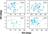 |
Fig. 1. Distribution of the stars analyzed in this letter (see Table 1) in the field of view of Kepler. |
Summary of the datasets used in this paper.
For fields C01 and C02, time series based on Simple Aperture Photometry (SAP) have been downloaded in ASCII format from the target inquiry page of the NASA Exoplanet Archive (IPAC). Field C03 and C04 time series data are not available at this site, but they are accessible through the ExoFOP link by the same host. To aid the method vital for filtering out instrumental systematics (TFA, Kovacs et al. 2005), in addition to the fundamental mode RR Lyrae (RRab) stars, 2–4 thousand stars were also downloaded for each field. These stars are distributed over the entire Kepler field of view and cover a wide range of brightnesses. All time series are of long cadence (i.e., with ~30 min sampling) and contain over 3000 data points with a continuous coverage of ~70 days.
It is well known that instrumental systematics are much more severe in the K2 phase of the Kepler mission than they were during the first phase with all four reaction wheels working. Therefore, correction for the various forms of systematics originating from this, and several other issues (e.g., ignition of thrusters) should be considered in the time series analysis. In the case of large amplitude variable stars, this correction (if it is made without full modeling of the data) may lead to disastrous results. We presume that this is the main reason why variability studies have so far largely avoided any filtering of systematics and have simply used carefully chosen aperture forms and only aperture photometry without any essential post-processing to obtain the best possible results (e.g., Plachy et al. 2017).
To search for astronomical signals and tackle systematics at the same time, without deforming the signal, Foreman-Mackey et al. (2015) and Angus et al. (2016) employed full models, whereas Aigrain et al. (2016) developed a method based on the flexibility of modeling with Gaussian Process. As discussed by Kovacs et al. (2016), when these methods are used for period search for signals commensurable with the size of the systematics, due to the extra freedom introduced by the inclusion of the underlying (but unknown) signal, the resulting detection statistics become poorer than for the more standard methods, assuming no signal content (e.g., SysRem of Tamuz et al. 2005).
The situation is different when the period of the dominating signal is known and we search for small secondary signals hidden in the systematics. The very simple methodology one can follow has been touched upon in some of our earlier papers (Kovacs et al. 2005; Kovacs & Bakos 2008). We described the method and illustrated its power through examples drawn from the K2 database in Kovacs (2018). For the sake of a more compact presentation, here we summarize the main steps of the analysis.
-
Choose NTFA co-trending time series {Uj(i); j = 1, 2, …, NTFA; i = 1, 2, …,N} from the stars available in the field (interpolate – if needed – to bring the target and the co-trending time series to the same timebase). We note that in this study, we selected these stars from the bright end of the available stars, but no other selections were made (e.g., on the basis of variability).
-
Derive the fundamental frequency f0 of the target {T(i); i = 1, 2, …, N} from the SAP time series.
-
Compute the sine and cosine values up to the NFOUR −1 harmonics of f 0: {Sj(i), Cj(i); j = 1, 2, …, NFOUR; i = 1, 2, …, N}.
-
Perform standard least squares minimization for a0, {aj} {bk, ck} on the following expression:
![Mathematical equation: $$ \mathcal{D}=\sum_{i=1}^{\mathrm{N}}[T(i)-F(i){]}^2, $$](/articles/aa/full_html/2018/06/aa33181-18/aa33181-18-eq1.gif) (1)
(1)
 (2)
(2)
-
Using the solution above, compute
 and find the new value of f0. Iterate on steps 3, 4, and 5 until convergence is reached.
 -
With the converged f0, compute the residual {R(i)} = T(i) − F(i); i = 1,2,…, N} and perform standard Fourier frequency analysis on {R(i)} with pre-whitening.
-
After reaching the noise level, use all frequencies (f0 and its harmonics, the new frequencies) and the co-trending time series to perform a grand fit according to step 4 (extended with the new frequencies).
We note that certain care must be taken at some steps of the analysis. For example, if the systematics are too large, then we need to perform a TFA analysis first, to derive a good estimate on f0 (we had one such a case in the dataset analyzed). Also, some frequency proximity condition should be applied, otherwise the fit may become unstable. We found that if the difference between the adjacent frequency values found during the pre-whitening process exceeded 0.1/T, the fit remained stable. Below this limit, we kept only one of the components.
3. Analysis, examples, and observed occurrence rate
We analyzed all 237 objects in Table 1 using the method described in Sect. 2. A wide frequency band of [0, 30] c/d was chosen to accommodate high harmonics. Even though the number of harmonics was high (14, throughout the analysis), in many cases leakage from the harmonics higher than the Nyquist frequency (24.47 c/d in the case of the present K2 data) caused a well-defined pattern from ~ 10 to 15 c/d. Our stoppage criterion for ending the pre-whitening cycle was a signal-to-noise ratio (S/N) of <6, where S/N = (A peak – 〈A〉)/σ(A), with A denoting the amplitude spectrum with sigma-clipped average 〈A〉 and standard deviation σ(A). The results presented in this paper are based on runs using 100 co-trending stars. We note that in the preliminary study we used 400 and we ended up with the same conclusion. In critical cases we used a different number of co-trending light curves, to make sure that the final classification is robust enough.
We show two examples on the performance of the method used in this paper. Figure 2 shows a case when the SAP data suffer from some easily visible systematics. Our focus of interest is the light curve labeled TFA(FOUR); this light curve is obtained after subtracting the best combination of the co-trending light curves from the SAP data (i.e.,  ; see Sect. 2). In principle, these data should contain only the modulated pulsation of the star. Indeed, the filtered light curve shows a very clean pattern of modulation. In comparison, it is also evident that although the standard Kepler pipeline (PDC-SAP, see Smith et al. 2012) helps to alleviate signal distortion to some degree, there are obvious remnants of systematics, leaving a less cleanly defined BL modulation on the filtered light curve.
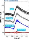 |
Fig. 2. An example from Campaign 3 on the performance of the filtering method used in this work in searching for secondary signal components. The light curves have been shifted vertically for better visibility. The lowermost light curve resulted from the subtraction of the large amplitude pulsation component (including the 14th harmonic) from the systematics-filtered TFA(FOUR) light curve. |
In another example in Fig. 3, we show the rare case of small systematics. Here we expect the method to leave the SAP signal basically intact. A brief visual inspection shows that it is indeed the case for the TFA(FOUR) light curve, but the filtering method employing a Gaussian Process model (K2SC, see Aigrain et al. 2016) apparently introduces additional noise in the data. These two examples show that employing a model best suited to the time series under scrutiny – in this case a periodic signal with a Fourier representation – greatly helps in the separation of systematics from the physically relevant signal content. Yet another important difference between our method and both of those mentioned above is the high number of co-trending time series used by TFA. In this way we can handle a large variety of systematics; unlike methods like PDC, that rely only on the leading PCA co-trending vectors.
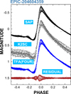 |
Fig. 3. An example from Campaign 2 on the performance of our method in the case of low level systematics. For comparison, the signal processing method based on a Gaussian Process model (K2SC, Aigrain et al. 2016), is also shown. |
The detection of the BL modulation is illustrated in Fig. 4. The upper panel shows the “easy” case: well-separated modulation side lobes with high amplitudes. The lower panel shows one of the cases with jammed power content at the fundamental frequency. In these cases, either the low modulation amplitude or the inherently complex nature of the modulation (or both) prevent a reliable estimation of the modulation period. Nevertheless, we also classified these cases as BL, due to the significant power content at the fundamental frequency.
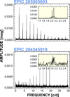 |
Fig. 4. Examples for high (upper panel) and low S/N (lower panel) detections. The amplitude spectra shown are the results of the DFT analysis of the TFA(FOUR) time series using the fundamental pulsation frequencies and their first 14 harmonics both in the TFA filtering and in the pre-whitening. The peaks come either from the BL side lobes or from the high-frequency components leaked through the Nyquist frequency at ~24.47 c/d. |
With multiple visual inspection of the frequency spectra of the 237 stars, we ended up with the following criterion for classifying a RRab star as a BL star: If at any stage of the pre-whitening cycle an excess of power occurs with S/N > 6 at a frequency f, satisfying |f – f 0| < 0.1 c/d, and this feature proves to be stable against changing the number of co-trending time series, then the star is classified as a BL star3. It is important to note that only about a dozen stars required closer examination in respect of this criterion. Once the side lobe/lobes is/are identified, two parameters were attached to the star to characterize its BL properties: (a) maximum side lobe amplitude, Am = max {Ai; 1, 2, …,Ns}, where {Ai} are the side lobe amplitudes (altogether Ns of them), and (b) the modulation frequency fm = f0 – f(Am). Please note that we selected these two parameters for the rough characterization of the BL stars, mainly to establish the distribution of A m, which is directly connected to the issue of detectability, the focus of this work.
As we have already mentioned, we found only 151 stars from the original set of 237 stars that can be classified as RRab stars. With the criterion mentioned, 138 of them proved to be BL stars. This implies 91 % observed occurrence rate, which is the highest value reported so far. The cumulative distribution function (CDF) of the observed maximum side lobe amplitudes is shown in Fig. 5. We see that some 40 % of the BL population originates from stars showing a relatively small modulation, under 0.002 mag4. It is also observed that the CDF has a break at ~0.0015 mag, suggesting perhaps two different populations of BL stars (or maybe even three, if we consider the further break suspected at the large {Am} limit of 0.03 mag5). Because of the importance of the population with low {Am}, in Fig. 6 we illustrate the actual observable light curve variations for two cases; in both cases the amplitude variations are not visible in the full-scale light curves, partially due to the long cadence of the data. Therefore, we zoomed to the upper envelopes in the middle and lower panels.
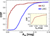 |
Fig. 5. Cumulative distribution function of the maximum side lobe amplitudes of the 138 BL stars identified in this work. For comparison, the same function is also shown for the 731 BL stars identified in the MACHO LMC sample by Alcock et al. (2003). The inset shows the blow-up of the region indicated in the main plot. |
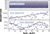 |
Fig. 6. Examples for small amplitude modulations from C03. Upper panel: light curve plotted on the scale of the full range of variation. Middle panel: zoom on the upper envelope. Lower panel: as in the middle panel, but for a star with a modulation period of 56 days. The gray lines are only for guiding the eyes in tracing the amplitude variation. |
4. The underlying rate
It is clear that the order of magnitude difference between the accuracy of the MACHO and K2 data should be an important source of the stunning difference in the observed {A m} distributions. Here we test the effect of the observational noise on the derived occurrence rates.
Our testbase for the K2 data is the set of 151 RRab stars analyzed in this paper. For the MACHO data, we use a larger set of non-BL (single period) RRab stars consisting of some 1700 stars from our earlier analysis in Alcock et al. (2003)6. The tests constitute the following steps. First, with the aid of an injected signal7 analysis, we check the detection rates at various test amplitudes. We use six different amplitudes both for the K2 and for the MACHO data and save the result for the occurrence rate test. The range of amplitudes ensures that for each star we have at least one detection. The frequency of the injected signal is placed at finj = 1.11 f0, close enough to the fundamental frequency, resembling the modulation side lobes, but far enough from it to avoid interaction with the side lobes already present in the data. The injected signal is labeled “detected” if the corresponding S/N is greater than 6.0 and the distance of the associated peak from the injected value is less than 0.5/T, where T is the total time span of the observations.
Because the estimation of the occurrence rate requires the knowledge of the detection likelihood for any amplitude given by the distribution of {Am}, we calibrate the test S/N values observed in the spectra (S/Nsp) with the analytical form of  via a simple scaling factor α
8. Figure A.1 shows the result of this calibration. We see that except for a negligible fraction of the test values, we can distinguish reliably for each star whether or not the injected signal was detectable.
via a simple scaling factor α
8. Figure A.1 shows the result of this calibration. We see that except for a negligible fraction of the test values, we can distinguish reliably for each star whether or not the injected signal was detectable.
Now we can use the observed {A m} distribution for the K2 data as shown in Fig. 5, and generate a large number of amplitudes and check if they are detectable in the stars of the sample. The results are summarized in Table 2.
Estimates on the observed occurrence rates.
In the first row, we show the observed rates. In the next three rows, we assume 100 % true occurrence rate, and impose various constraints on the injected signal amplitude. In the simplest case, we assume that each star has an equal probability of sampling the full range of modulation amplitudes according to the observed distribution on the K2 dataset. This assumption leads to a significant underestimation of the observed K2 rate. An obvious guess for a possible source of the underestimation is that the (unknown) dependence of the BL phenomenon on the stellar parameters cuts out low-amplitude modulations for specific parameter combinations. We tested this possibility by examining the period dependence of the modulation amplitudes. Figure A.2 shows that indeed, at short periods, we have an apparent lack of BL stars. Applying the constraints imposed by the lines labeled “a”, we get an increase (see third row); but it is still insufficient to reproduce the observed rate for the K2 data. Shrinking further the allowed region (case b) we arrive to a nice match for the K2 data. We note that at this level we have no knowledge of the actual parameter space of the BL phenomenon. This might be more complicated than the one used here (i.e., a simple smooth amplitude cut); therefore, the deeper cut seen in case b could be less severe, as it might seem from the several outliers in Fig. A.2 for this particular cut.
Because of the higher noise level of the MACHO data, they yield roughly the same, slightly discrepant value, independently of the restrictions posed on the modulation amplitude. It seems that the only way to reach the observed value is to decrease the underlying occurrence rate. Indeed, as shown in the last three rows of Table 2, assuming 90 % true rate yields the desired rate for the MACHO/LMC data. Unfortunately, the lower rate completely spoils the fine agreement for the K2 data. This may imply some real difference in the BL occurrence rates between the LMC and the Galactic field.
5. Conclusions
We analyzed 151 RR Lyrae stars from the K2 fields C01–C04, classified earlier by Armstrong et al. (2016) as fundamental mode (RRab) stars, and searched for Blazhko variability, generally characterized by a dense frequency spectrum near the fundamental mode. Our analysis adapts the method used widespread in the field of transiting extrasolar planets to filter out systematics from ground- and space-based data. These systematics act as colored noise in the frequency analysis, and falsify the result for signals with amplitudes similar to those of the systematics. The modified method takes into consideration the large amplitude component (stellar pulsation) of the RRab signal and maintains its shape with a simultaneous systematics filtering.
We report an occurrence rate of 91 % for the Blazhko phenomenon among the stars analyzed. This is the highest rate detected so far. After correcting for observational bias due to finite observational accuracy, we find that the underlying (true) rate should be very close to 100 % in the part of the Galactic field covered by C01–C04. This high true rate is confirmed by a similar debiasing applied to the MACHO data on LMC (Alcock et al. 2003), although the optimum rate turned out to be closer to 90 % for this dataset. The cumulative distribution function of the modulation side lobe amplitudes has a clear break at 0.0015 mag, leading to a conjecture on the possibility of the existence of a different subclass of Blazhko stars at small modulation amplitudes. Due to the very common nature of the Blazhko phenomenon and the narrowness of the stellar parameter regime satisfying radial resonance conditions (Kolláth et al. 2011), it seems likely that ideas employing radial mode resonances will face difficulties in explaining this level of commonality.
Acknowledgments
I thank David Armstrong for a quick reply to my inquiry on the data availability. I also appreciate the information on the analysis of the WASP data given by Paul Greer. Special thanks are due to Eric Petigura for making the K2 time series data available to the community in simple format through the IPAC ExoFOP site. This research has made use of the NASA Exoplanet Archive, which is operated by the California Institute of Technology, under contract with the National Aeronautics and Space Administration under the Exoplanet Exploration Program.
Appendix A: Figures related to the estimation of the underlying incidence rates
These figures are associated with the tests made in Sect. 4 to estimate the underlying (true) incidence rates of the Blazhko stars in various datasets. Please consult Sect. 4 for the appropriate contexts of these figures in applying the bias corrections to the observed rates.
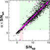 |
Fig. A.1. Detected S/N (S/Nsp) in the Fourier spectra vs. the calibrated analytical S/N (S/Nan). Each star is characterized by its own calibration factor α and (S/Nan). The calibration has been derived from injected signal tests, as described in the text. The MACHO and K2 stars are plotted by black and magenta, respectively. Pale green and red rectangles denote the parameter regimes where the two S/N estimates yield consistent and inconsistent detection results, respectively. |
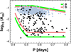 |
Fig. A.2. Observed modulation amplitudes (Fourier amplitudes – in [mag] – of the largest side lobes in the vicinity of the frequency of the fundamental mode) vs. pulsation period. Black dots represent the K2 sample of this work, whereas pale dots represent the Blazhko stars from the MACHO survey of Alcock et al. (2003). The various bounds of the region denoted by a and b are used in the estimation of the underlying occurrence rates. |
The only exception is perhaps the discovery of the alternation of the maxima in certain phases of the Blazhko cycle, which is currently attributed to a high-order resonance involving the fundamental mode – see Buchler & Kolláth (2011) and Smolec (2016) for some critical comments.
The types of misclassifications cover objects such as binaries, RRc stars, multiperiodic, rotational and irregular variables, noise, etc.
The 0.1 c/d upper limit for the modulation frequency fm is supported by the small number of BL stars with fm > 0.1 c/d – see Greer et al. (2017) and the lack of such stars in the dataset analyzed in this paper.
It is recalled that this is the size of the largest side lobe. Because additional components are frequently present, the total amplitude of the modulation is, in general, larger.
Let us note that the low amplitude part of the CDF is biased, due to the likely underestimation of A m for long modulation periods.
We aim at a larger statistical sample, therefore we employ the subset of the non-BL stars. By using the BL stars, we get the same result.
Importantly, we inject the test signal in the SAP data and proceed as with the real (observed) data. Injecting the test signal in the TFA-filtered data would falsify (i.e., increase) our detection rates, because of the considerably lower noise resulting from the filtering.
Because of the importance of the low-S/N regime, we weight heavily (proportionally to  ) these values in the least squares fit for α.
References
- Aigrain, S., Parviainen, H., & Pope, B. J. S. 2016, MNRAS, 459, 2408 [NASA ADS] [Google Scholar]
- Alcock, C., Alves, D. R., Becker, A., et al. 2003, ApJ, 598, 597 [NASA ADS] [CrossRef] [Google Scholar]
- Angus, R., Foreman-Mackey, D., & Johnson, J. A. 2016, ApJ, 818, 109 [NASA ADS] [CrossRef] [Google Scholar]
- Armstrong, D. J., Kirk, J., Lam, K. W. F., et al. 2016, MNRAS, 456, 2260 [NASA ADS] [CrossRef] [Google Scholar]
- Benkő, J. M., Plachy, E., Szabó, R., et al. 2014, ApJS, 213, 31 [NASA ADS] [CrossRef] [Google Scholar]
- Blazhko, S. 1907, Astron. Nachr., 175, 325 [NASA ADS] [CrossRef] [Google Scholar]
- Buchler, J. R., & Kolláth, Z. 2011, ApJ, 731, 24 [NASA ADS] [CrossRef] [Google Scholar]
- Christy, R. F. 1964, Rev. Mod. Phys., 36, 555 [NASA ADS] [CrossRef] [Google Scholar]
- Foreman-Mackey, D., Montet, B. T., Hogg, D. W., et al. 2015, ApJ 806, 215 [NASA ADS] [CrossRef] [Google Scholar]
- Greer, P. A., Payne, S. G., Norton, A. J., et al. 2017, A&A, 607, A11 [NASA ADS] [CrossRef] [EDP Sciences] [Google Scholar]
- Jurcsik, J., Sódor, Á., Szeidl, B., et al. 2009, MNRAS, 400, 1006 [NASA ADS] [CrossRef] [Google Scholar]
- Kolláth, Z., Molnár, L., & Szabó, R. 2011, MNRAS, 414, 1111 [NASA ADS] [CrossRef] [Google Scholar]
- Kovacs, G. 2016, CoKon, 105, 61 [Google Scholar]
- Kovacs, G. 2018, Proc. Polish Astron. Soc., [arXiv:1804.01894] [Google Scholar]
- Kovacs, G., & Bakos, G. A. 2008, Commun. Asteroseismol., 157, 82 [Google Scholar]
- Kovacs, G., Bakos, G., & Noyes, R. W. 2005, MNRAS, 356, 557 [NASA ADS] [CrossRef] [Google Scholar]
- Kovacs, G., Hartman, J. D., Bakos, G. A., et al. 2014, MNRAS, 442, 2081 [NASA ADS] [CrossRef] [Google Scholar]
- Kovacs, G., Hartman, J. D., & Bakos, G. A. 2016, A&A, 585, A57 [CrossRef] [EDP Sciences] [Google Scholar]
- Petigura, E. A., Schlieder, J. E., Crossfield, I. J. M., et al. 2015, ApJ, 811, 102 [NASA ADS] [CrossRef] [Google Scholar]
- Plachy, E., Klagyivik, P., Molnár, L., et al. 2017, EPJ Web of Conf., 160, 04009 [Google Scholar]
- Shapley, H. 1916, ApJ, 43, 217 [NASA ADS] [CrossRef] [Google Scholar]
- Smith, J. C., Stumpe, M. C., Van Cleve, J. E., et al. 2012, PASP, 124, 1000 [NASA ADS] [CrossRef] [Google Scholar]
- Smolec, R. 2016, Proc. Polish Astron. Soc., 3, pp.22 [Google Scholar]
- Szabó, R., Benkő, J. M., Paparó, M. 2014, A&A, 570, A100 [NASA ADS] [CrossRef] [EDP Sciences] [Google Scholar]
- Tamuz, O., Mazeh, T., & Zucker, S. 2005, MNRAS, 356, 1466 [NASA ADS] [CrossRef] [Google Scholar]
All Tables
All Figures
|
Fig. 1. Distribution of the stars analyzed in this letter (see Table 1) in the field of view of Kepler. |
| In the text | |
|
Fig. 2. An example from Campaign 3 on the performance of the filtering method used in this work in searching for secondary signal components. The light curves have been shifted vertically for better visibility. The lowermost light curve resulted from the subtraction of the large amplitude pulsation component (including the 14th harmonic) from the systematics-filtered TFA(FOUR) light curve. |
| In the text | |
|
Fig. 3. An example from Campaign 2 on the performance of our method in the case of low level systematics. For comparison, the signal processing method based on a Gaussian Process model (K2SC, Aigrain et al. 2016), is also shown. |
| In the text | |
|
Fig. 4. Examples for high (upper panel) and low S/N (lower panel) detections. The amplitude spectra shown are the results of the DFT analysis of the TFA(FOUR) time series using the fundamental pulsation frequencies and their first 14 harmonics both in the TFA filtering and in the pre-whitening. The peaks come either from the BL side lobes or from the high-frequency components leaked through the Nyquist frequency at ~24.47 c/d. |
| In the text | |
|
Fig. 5. Cumulative distribution function of the maximum side lobe amplitudes of the 138 BL stars identified in this work. For comparison, the same function is also shown for the 731 BL stars identified in the MACHO LMC sample by Alcock et al. (2003). The inset shows the blow-up of the region indicated in the main plot. |
| In the text | |
|
Fig. 6. Examples for small amplitude modulations from C03. Upper panel: light curve plotted on the scale of the full range of variation. Middle panel: zoom on the upper envelope. Lower panel: as in the middle panel, but for a star with a modulation period of 56 days. The gray lines are only for guiding the eyes in tracing the amplitude variation. |
| In the text | |
|
Fig. A.1. Detected S/N (S/Nsp) in the Fourier spectra vs. the calibrated analytical S/N (S/Nan). Each star is characterized by its own calibration factor α and (S/Nan). The calibration has been derived from injected signal tests, as described in the text. The MACHO and K2 stars are plotted by black and magenta, respectively. Pale green and red rectangles denote the parameter regimes where the two S/N estimates yield consistent and inconsistent detection results, respectively. |
| In the text | |
|
Fig. A.2. Observed modulation amplitudes (Fourier amplitudes – in [mag] – of the largest side lobes in the vicinity of the frequency of the fundamental mode) vs. pulsation period. Black dots represent the K2 sample of this work, whereas pale dots represent the Blazhko stars from the MACHO survey of Alcock et al. (2003). The various bounds of the region denoted by a and b are used in the estimation of the underlying occurrence rates. |
| In the text | |
Current usage metrics show cumulative count of Article Views (full-text article views including HTML views, PDF and ePub downloads, according to the available data) and Abstracts Views on Vision4Press platform.
Data correspond to usage on the plateform after 2015. The current usage metrics is available 48-96 hours after online publication and is updated daily on week days.
Initial download of the metrics may take a while.