| Issue |
A&A
Volume 614, June 2018
|
|
|---|---|---|
| Article Number | A53 | |
| Number of page(s) | 16 | |
| Section | Stellar structure and evolution | |
| DOI | https://doi.org/10.1051/0004-6361/201732076 | |
| Published online | 12 June 2018 | |
Episodic accretion in binary protostars emerging from self-gravitating solar mass cores
1
Departamento de Astronomía, Facultad Ciencias Físicas y Matemáticas, Universidad de Concepción,
Av. Esteban Iturra s/n Barrio Universitario,
Casilla
160-C,
Concepción, Chile
e-mail: This email address is being protected from spambots. You need JavaScript enabled to view it.
,This email address is being protected from spambots. You need JavaScript enabled to view it.
2
Centre for mathematical Plasma-Astrophysics, Department of Mathematics, KU Leuven,
Celestijnenlaan 200B,
3001
Heverlee, Belgium
e-mail: This email address is being protected from spambots. You need JavaScript enabled to view it.
Received:
10
October
2017
Accepted:
25
December
2017
Abstract
Observations show a large spread in the luminosities of young protostars, which are frequently explained in the context of episodic accretion. We tested this scenario with numerical simulations that follow the collapse of a solar mass molecular cloud using the GRADSPH code, thereby varying the strength of the initial perturbations and temperature of the cores. A specific emphasis of this paper is to investigate the role of binaries and multiple systems in the context of episodic accretion and to compare their evolution to the evolution in isolated fragments. Our models form a variety of low-mass protostellar objects including single, binary, and triple systems in which binaries are more active in exhibiting episodic accretion than isolated protostars. We also find a general decreasing trend in the average mass accretion rate over time, suggesting that the majority of the protostellar mass is accreted within the first 105 years. This result can potentially help to explain the surprisingly low average luminosities in the majority of the protostellar population.
Key words: stars: formation / methods: numerical / accretion, accretion disks
© ESO 2018
1 Introduction
Understanding the non-linear dynamics of star formation poses a significant challenge. During protostellar collapse, the gas that is part of the interstellar medium experiences a more than ten orders of magnitude increase in density. However, despite the challenges, non-linear phenomena such as episodic accretion can potentially explain some observed inconsistencies that are related to the luminosity of young low-mass protostars (Kenyon et al. 1990). For example, if there is a constant flow of matter from a collapsing envelope of gas onto protostars, we would expect that a sample of these low-mass objects should have the same luminosities, but instead observations have shown that low-mass protostars indeed have different luminosities (Fischer et al. 2017). In fact, a range of observed protostellar luminosities distribution from 0.01 L⊙ to 69 L⊙ with a median of 1.3 L⊙ has been reported (Dunham et al. 2013). Similarly, if the mass supply to the protostars from a depleting envelope gets reduced, their luminosities should also be reduced so that a T Tauri star should not be more luminous than protostars that are still in their embedded phase of collapse. The observations, however, clearly do not follow this prediction (Dunham et al. 2008; Fischer et al. 2013).
A variety of initial conditions are present in star forming regions (Girichidis et al. 2012). Observations have also revealed a considerable diversity in the morphology of young and developed star systems (Chen et al. 2015; Megeath et al. 2015). When investigated using numerical models, this diversity in the morphology of the systems has been found to be highly dependent on the initial conditions prevailing in star forming gas (Vanajakshi & Jenkins 1984; Sigalotti & Klapp 2000; Jessop & Ward 2001; Khesali et al. 2013; Bate et al. 2014). The great number of physical parameters involved in setting the initial conditions in molecular cloud cores makes the phenomenon of star formation interesting as well as complex enough to explore in every detail. In addition to physical processes such as episodic accretion onto young embedded protostars (Fendt 2009), many other exciting features of star formation exist, such as protostellar jets (Vorobyov & Basu 2015; Lee 2015) observed during the accretion phase of protostars (Whelan et al. 2014) and in the absence of efficient angular momentum transport mechanisms (Attwood et al. 2009; Walch et al. 2012). The fundamental cause of episodic accretion is still unclear (Stamatellos et al. 2012).
Many authors from Herbig (1997) to Visser et al. (2015) have suggested the possibility of accretion via bursts that may last for relatively short durations within the range of timescales spanning a few tens to a hundred years. This was recently confirmed by performing zoom simulations with the adaptive mesh-refinement code RAMSES (Küffmeier et al. 2018). The possibility of episodic mass inflow has also been found to be important in another phase of protostellar evolution known as the episodic molecular outflow phase (Plunkett et al. 2015).
Machida et al. (2010) conducted a numerical study in which long-term simulations of the main accretion phase of star formation were carried out. They observed that spiral density waves are an important factor contributing to the strong time variability of the mass accretion rate onto protostars. These authors found that the time variability of the accretion rate is lower in clouds with lower initial rotational energy. Their results suggest a dependence of the mass accretion rate on the initial rate of rotation of a molecular core. Our simulations complement these previous findings by focusing on additional parameters that may also dictate the history of the mass accretion rates.
A large ensemble of simulations of collapsing and fragmenting cores has been performed by Lomax et al. (2014) to understand the observed characteristics of star formation in the Ophiuchus cloud. In this work they explored three types of models (i.e., no radiative feedback, continuous radiative feedback, and episodic radiative feedback) that affect fragmentation and the resulting protostellar masses. While their simulations without radiative feedback produced too many brown dwarfs, those with continuous radiative feedback yielded too few brown dwarfs. However, with episodic radiative feedback both the peak of the protostellar mass distribution at ~0.2 M⊙ and the ratio of H-burning stars to brown dwarfs was found to be consistent with the observations.
While analyzing the evolving protostars in simulations we focus on how episodic accretion plays a possible role in the formation ofmultiple low-mass protostellar systems exhibiting vigorous mass accretion rates that may introduce even more complexity to the phenomenon of competitive mass accretion. To be able to follow collapsing systems on a sufficiently long timescale, we use a sink particle scheme combined with the well-known smoothed particle hydrodynamics (SPH) method. The sink particlescheme replaces self-gravitating high density peaks within the collapsing gas with particles that only feel the gravitational influence of other mass-carrying particles in the simulation. Once a sink is created the material is allowed to flow smoothly toward the sink and can be accreted by the sink particle according to a set of rules that mimic accretion onto protostars as closely aspossible (Richtmyer & Morton 1994). In a similar way, the sink particle scheme can also be used to simulate accretion onto binaries and multiple stellar systems. In this way the sink particles act as subgrid models for protostars without having to calculate their internal evolution in any detail. This strategy allows us to follow the detailed collapse of molecular cloud cores without suffering from the limitations imposed by ever decreasing time steps associated with growing densities within protostars as explained by Richtmyer & Morton (1994). The sink particle approach has been implemented in both Eulerian and Lagrangian numerical codes based on the AMR and SPH methods (Hubber et al. 2013; Federrath et al. 2010; Hocuk & Spaans 2011). The sink particle scheme also enables us to analyze the physical processes going on in near protostellar clumps and allows us to study possible episodic accretion onto the sink particles along with their effects on nearby gas and other condensations in their vicinity.
The previous paragraphs contain the motivation and background for the numerical study presented in this paper. We have attempted to model the initial stages of the formation of systems composed of very low-mass (VLM) stars evolving within a common envelope of gas. Our models start with molecular cloud cores with varying initial temperatures and associated sound crossing times. These cores are also seeded with non-axisymmetric density perturbations of varying strength to mimic the presence of large scale turbulence on the level of molecular cloud cores. We find that the models give rise to a variety of outcomes. Our results include, for example, both multiple and single protostellar systems each consisting of VLM protostars. Among the multiple protostellar systems we find both close and wide binaries. Some of these binary systems exhibit signs of episodic accretion. In addition to VLM binaries we also find VLM triplets that include binary systems as one of their components.
The plan of the paper is as follows. Section 2 discusses the computational scheme. In Sect. 3 we describe the initial conditions and setup for our models. Section 4 discusses the equation of state used in our models. Section 5 briefly explains the treatment of self-gravitating clumps and a reference to the scheme adopted to compute binary properties. Section 6 then provides a detailed account of our results and finally we present our conclusions in Sect. 7.
2 Computational scheme
The numerical models presented in this paper are based on the particle simulation method known as smoothed particle hydrodynamics (SPH). We used the computer code GRADSPH developed by Vanaverbeke et al. (2009). The GRADSPH code is a fully three-dimensional SPH code that combines hydrodynamics with self-gravity and has been specially designed to study self-gravitating astrophysical systems such as molecular clouds. The numerical scheme implemented in GRADSPH implements the long range gravitational interactions within the fluid by using a tree-code gravity (TCG) scheme combined with the variable gravitational softening length method (Price & Monaghan 2007), whereas the short range hydrodynamical interactions are solved using a variable smoothing length formalism. The code uses artificial viscosity to treat shock waves.
In SPH, the density ρi at the position ri of each particle with mass mi is determined by summing the contributions from its neighbors using a weighting function W(ri −rj, hi) with smoothing length hi as follows:
 (1)
(1)
The GRADSPH code uses the standard cubic spline kernel with compact support within a smoothing sphere of size 2hi (Price & Monaghan 2007). The smoothing length hi itself is determined using the following relation:
 (2)
(2)
where η is a dimensionless parameter that determines the size of the smoothing length of the SPH particle given its mass and density. This relation is derived by requiring that a fixed mass, or equivalently a fixed number of neighbors, must be contained inside the smoothing sphere of each each particle and is written as
 (3)
(3)
Here Nopt denotes the number of neighbors inside the smoothing sphere, which we set equal to 50 for the three-dimensional simulations reported in this paper. Substituting Eq. (2) into Eq. (3) allows us to determine η:
 (4)
(4)
Since Eqs. (1) and (2) depend on each other, we solve the two equations iteratively at each time step and for each particle.
The evolution of the system of particles is computed using the second-order predict-evaluate-correct (PEC) scheme implemented in GRADSPH, which integrates the SPH form of the equations of hydrodynamics with individual time steps for each particle. For more details and a derivation of the system of SPH equations we refer to Vanaverbeke et al. (2009).
3 Initial conditions and setup
In the present study we used a modified version of the Boss and Bodenheimer collapse test with initial conditions described in Burkert & Bodenheimer (1993). The overall setup of the initial conditions is identical to the cloud core models that we used previously while investigating the thermal response of collapsing molecular cores (Riaz et al. 2014). We maintained the m = 2 non-axisymmetric density perturbations with a fixed amplitude A that varies from model to model. We introduced identical amplitudes of the azimuthal density perturbation in each hemisphere of the uniform density core models. This perturbation is designed to approximately include the effect of large scale turbulence on the scale of giant molecular clouds, which can induce asymmetric density distributions in embedded molecular cores that are on the verge of gravitational collapse. For this purpose we used the following form of the density perturbation:
 (5)
(5)
where φ is the azimuthal angle in spherical coordinates (r, φ, z).
Our solar mass molecular cloud core models with an initial temperature of 8 K have dimensionless ratios of Jeans mass to initial core mass, thermal energy to magnitude of gravitational energy, and rotational energy to the magnitude of the gravitational potential energy equal to 0.143, 0.264, and 0.0785, respectively. Models with other initial thermal states have corresponding values for these ratios. While we explore a certain range of parameters, we also emphasize that statistically significant trends can only be derived after exploring a more extensive range of possible realizations for the initial conditions. While our results may provide hints toward possible trends or general phenomena, we do not intend to derive strict relations. We emphasize that the current paper thus provides only a first step and a much larger range of initial conditions needs to be explored in the future.
4 Equation of state
The chemical composition of the clouds is similar our previously studied models (Riaz et al. 2014). We assume the gas to be a mixture of hydrogen and helium with mean molecular weight μ = 2.35. The initial temperature T0 is chosen as 8 K for the models labeled M1, M2, M3, and M4 presented in this paper. The corresponding sound speed is cs = 167.62 m s−1 and the initial free fall time is tff = 1.07 × 10¹² s or 3.4 × 10⁴ yr. Furthermore, the sound speed takes different values for models M5 and M6 as we varied the initial thermal state of the molecular core by setting the initial temperature to 10 K and 12 K, respectively. We adopted a barotropic equation of state of the form
![Mathematical equation: \begin{equation*}P=\rho c_{0}^{2}\left[1+\left(\frac{\rho}{\rho_{crit}}\right)^{\gamma-1}\right], \vspace*{-6 pt} \end{equation*}](/articles/aa/full_html/2018/06/aa32076-17/aa32076-17-eq6.png) (6)
(6)
in which γ = 5∕3. This approximate equation of state describes the gradual transition from isothermal to adiabatic behavior of the gas during gravitational collapse. For the critical density ρcrit we used a value of 10−13 g cm−3, which is slightly higher than the value of 10−14 g cm−3. An overviewof the models is provided in Table 1. The table contains the properties of the initial conditions and relevant information on the final outcome of their evolution. By adopting various values for the azimuthal density perturbation amplitudes while keeping the rest of the initial parameters identical for models M1–M4, and testing different initial thermal states for models M5 and M6, we aim to investigate the role of primary/secondary fragmentation in the formation of VLM stars. By primary fragmentation we mean the break up of a cloud into initial fragments as the direct result of the imposed perturbation, whereas secondary fragmentation mainly takes place in later stages during the course of the further evolution of the system. This strategy gives us the opportunity to analyze numerically the properties of weak or strong primary fragmentation. Primary fragmentation can control the mass accretion process onto secondary condensations and hence can dictate the eventual outcome of the collapse. While varying the perturbation strengths and the initial thermal states, we studied the mass ratio, eccentricity, binary separation, and type of binary companion of the resulting binary systems. We also look at the rate of accretion of individual fragments and the number of primary/secondary fragments in the embedded phase of core collapse.
We note again that the relations that result from this investigation need to be regarded with a grain of salt and should be tested in future studies employing a larger range of initial conditions.
5 Treatment of self-gravitating clumps
In order to deal with self-gravitating clumps in our simulations, we took advantage of the recently proposed improved sink particle algorithm for SPH calculations described by Hubber et al. (2013). We introduced sinks into the version of GRADSPH used in this paper following the algorithm NEWSINKS by Hubber et al. (2013, see Sect. 2) in which a SPH particle can be turned into a sink with accretion radius rsink once its density exceeds a given threshold ρsink. For the present simulations we adopted the values ρsink= 10−10 g cm−3 and rsink = 1.0 au, respectively.The criteria for sink particle creation and accretion of SPH particles within the accretion radius follow Sects. 2.2 and 2.3 in Hubber et al. (2013), respectively. Because the mechanism for angular momentum transfer in accretion disks is still uncertain, we decided not to implement angular momentum feedback from sink particles.
We took advantage of a scheme discussed by Stacy & Bromm (2013) in their Sect. 2.5 to compute binary properties of sinks emerging in our simulations.
6 Results and discussion
We now state the results of our simulations and discuss these systematically.
6.1 Dependence on perturbation amplitude
We intend to investigate how the first fragments that form in our simulations affect the later secondary fragmentation processes within disks orbiting protostars. The fragments that appear as a result of the initial perturbation with azimuthal dependence depending on the mode m and the amplitude A are designated as primary fragments. On the other hand, clumps that emerge because of gravitational instabilities arising in evolving disks within the core at a later stage and are not directly connected to the initial perturbation are regarded as secondary fragments.
The evolution of model M1 is illustrated in Fig. 1. The plots are face-on column density plots along the rotation axis at six successive times during the evolution of the model. Two primary fragments (sink 1 and sink 2) emerge at 42.40 kyr and 42.51 kyr, respectively. As the system evolves further, it gives birth to four additional secondary fragments (sink 3, sink 4, sink 5, and sink 6), which appear at 42.58 kyr, 42.59 kyr, 42.94 kyr, and 42.99 kyr, respectively. The small amplitude of the initial density perturbation A = 0.005 in this model does not seem to favor the primary fragments in terms of mass accumulation and all primary and secondary fragments eventually accrete enough material from the envelope to become VLM stars. Panel b shows that some of the protostars form close binary systems as depicted by the zoomed in part of the panel. There is also a triplet system indicated by an arrow in panel f, which includes a close binary system.
We have not followed the dynamics of this system further in time primarily because of computational constraints such as time steps that are too small. Nevertheless, there are indications that the development of such an initially compact triplet could result in the formation of a wide binary system, provided that there is not much gas available for dynamical friction to shrink the binary separation, on a timescale of millions of years as one component is migrated to a distant orbit at the cost of shrinking the orbits of the other two components in the system (see, e.g., Reipurth & Mikkola 2012; Law et al. 2010). The presence of a relatively small initial perturbation in model M1 seems to support the formation of a relatively large number of sinks. Furthermore, the triplet system that is formed during the evolution of this model only consists of secondary fragments. By the time the simulation ends at t = 3.00 tff, in addition to an unbound primary, the binary (primary-secondary) and the triplet (secondaries) are left as gravitationally bound systems embedded within the collapsing gas with binary separations of 28.61 au and 25.00 au and mass ratios of 0.752 and 0.93, respectively, for the two bound systems as summarized in Tables 1 and 4.
Figure 2 shows the evolution of model M2. In this model the strength of the initial density perturbation increases by a factor of 10 compared to model M1. The two primary fragments (sink 1 and sink 2) emerge in this model at 42.70 kyr and 42.76 kyr, respectively. Further gravitational collapse of the core produces additional secondary fragments (sink 3, sink 4, and sink 5) at 43.13 kyr, 43.94 kyr, and 46.47 kyr, respectively.
In model M2 we find a binary system composed of sink 2 and sink 4, i.e., a (primary-secondary) combination. The binary separation at this stage is 46.48 au and the eccentricity of the system is 0.22 (see Table 4).
Figure 3 presents the evolution of model M3 in which the level of the initial density perturbation is further increased bya factor of 2. In this case the primary fragments are clearly able to accrete a significant percentage of the gas present in the collapsing core. The two primary fragments (sink 1 and sink 2) appear at 40.64 kyr and 44.46 kyr, respectively. Thereafter, three more secondary fragments are formed (sink 3, sink 4, and sink 5) at core evolution times 44.87 kyr, 46.78 kyr, and 52.25 kyr, respectively. In this model one could expect to observe an enhanced mass contrast among the fragments that could lead to the formation of VLM stars, brown dwarfs, or even planetary-mass objects (planemos), but this trend does not seem to prevail and decide the outcome of the core collapse. The evolution of this model yields four VLM stars that form two close binaries with binary separations of 30.53 au and 38.47 au, respectively. In addition to these close binaries there is also a single protostar that is unbound with respect to the nearby binary systems. Compared to model M1, the total number of fragments roughly remains the same. At the end of the simulation at t = 2.998 tff, the system again contains a single VLM star and a couple of VLM binary systems that are a combination of primary-secondary and secondary-secondary fragments (see Table 4).
Finally, Fig. 4 illustrates the evolution of model M4 in which the amplitude of the initial density perturbation is set to 0.2.This is the highest value of the amplitude of the initial density perturbation in any of our simulations (see Table 1). Two primary fragments (sink 1 and sink 2) appear in this model at 41.44 and 41.55 kyr, respectively. This is then followed by the formation of two additional secondary fragments (sink 3 and sink 4) which appear at 50.26 and 57.48 kyr, respectively. Ultimately a triple VLM star system is formed which includes a primary-secondary binary system with a binary separation of 56.30 au (see Table 4). In addition to the triple VLM star system, there is also a single protostar which remains unbound with respect to the triple star system until the end of the simulation at t = 5.401 tff.
 |
Fig. 1 Results of the simulation for model M1. The physical size of each individual panel is 4333 × 4333 au. The plots show face-on views of the column density integrated along the rotation axis(z) at 6 successive times during the evolution of the model. The color bar on the right shows log (Σ) in dimensionless units. Each calculation was performed with 250025 SPH particles. |
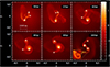 |
Fig. 2 Results of the simulation for model M2. The physical size of each individual panel is 4333 × 4333 au. The plots show face-on views of the column density integrated along the rotation axis(z) at 6 successive times during the evolution of the model. The color bar on the right shows log (Σ) in dimensionless units. Each calculation was performed with 250025 SPH particles. |
6.2 Dependence on initial temperature
We now turn to the effect of increasing the temperature of the core. In model M5, we raised the initial temperature by 2 K to study the effect of a shorter sound crossing time and a higher initial thermal state on the collapse. The remainder of the model parameters were identical to model M2. The results are reported in Fig. 5. The primary fragments (sink 1 and sink 2) are formed at 45.69 kyr and 45.96 kyr, respectively. Two secondary fragments emerge as sink 3 and sink 4 at 46.09 kyr and 63.37 kyr. Compared to model M2, model M5 takes a longer time to give birth to the last fragment in the core. Although the density perturbation is relatively modest, the change in initial temperature greatly alters the outcome of this model. At the end of the simulation for model M5 at t = 7.307 tff, two binary systems with components of identical nature have appeared. One is a very close VLM binary composed of two secondary fragments with binary separation and mass ratio of 28.180 au and 0.496, respectively, while the other is a relatively wide VLM binary including two primary fragments and with binary separation and mass ratio of 231.50 au and 0.723, respectively. The binding energy of the secondary-secondary binary is much greater than for the primary-primary binary since both have a similar mass and the primary-primary has a much wider separation.
Figure 6 illustrates the development of the last model M6 where the initial temperature has been further increased by 2 K compared to model M5. As expected, the increase in the thermal energy content of the collapsing molecular core delays the fragmentation process. This is directly related to how the temperature change affects the Jeans mass at the density of fragmentation (Tohline 1980). The Jeans mass at density ρ and temperatureT can be expressed as
 (7)
(7)
Equation (7) shows that for a given density, the Jeans mass takes on larger values at higher temperatures so that for any potential fragment, it therefore takes a relatively longer time to reach the threshold above which gravitational collapse occurs.
The two primary fragments emerge within the collapsing cloud as sink 1 and sink 2 at 51.78 kyr and 56.01 kyr, respectively. This is followed by the appearance of a third and last fragment (sink 3) 57.05 kyr after the start of the collapse. The presence of only three fragments after 0.162 Myr of evolution clearly shows that gravity is partly balanced by the thermal pressure exerted by the gas. Model M6 evolves into a protobinary system of the primary-primary type with binary separation and mass ratio equal to 110.50 au and 0.858, respectively, and there is also one single VLM star. Although we did not run a statistically significant number of simulations to be able to perform a thorough analysis of the properties of the binaries that are formed in our models, we find interesting differences between the two sets of models (M1, M3, and M4) and (M2, M5, and M6). On the one hand, all of the binaries formed in the first set are composed of a combination of primary and secondary fragments. On the other hand, all of the binaries formed in the second set of models are either a combination of two primary fragments or two secondary fragments (see Table 4 for details). Future work will be needed to explore in more detail if such a relation can indeed be confirmed.
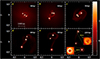 |
Fig. 3 Results of the simulation for model M3. The physical size of each individual panel is 4333 × 4333 au. The plots show face-on views of the column density integrated along the rotation axis(z) at 6 successive times during the evolution of the model. The color bar on the right shows log (Σ) in dimensionless units. Each calculation was performed with 250025 SPH particles. |
Summary of the initial physical parameters and the final outcome of the models discussed in this paper.
Summary of the final evolution time tf, total number of fragments Ntot, masses of the fragments (in the order as they appear in the simulation), and number of *bound* objects (VLM stars) Nbound at the end of the simulation.
Summary of the maximum evolution time in units of the initial free fall time tff, and final ratio of the envelope mass to the initial mass of cloud core for models M1–M6.
Summary of the models, type of the fragments which are components of binaries, masses of the components, mass ratio (q), semimajor axis (a), eccentricity (e), and binary separation (d) at the end of each run.
6.3 Evolution of clump masses and accretion rate
In a recent study reported by Vorobyov & Basu (2010), the properties of prestellar cores that make core disks susceptible to fragmentation have been analyzed. These authors found that a higher initial core angular momentum and a higher core mass lead to more fragmentation, while higher levels of background radiation and magnetic fields moderate the tendency of the disk to fragment.On the other hand, the simulations reported here focus on how primary and secondary fragmentation takes place within the core disks and allow us to study the dependence of these phenomena on initial conditions with varying initial density perturbations and varying initial thermal states. With this goal in mind, Fig. 7 shows the evolution of the total mass contained within the primary fragments (dashed lines) and the secondary fragments (dotted lines), along with the remaining mass in the envelope surrounding the fragments for models M1–M6 (full lines). Comparing models M1, M2, M3, and M4 shows that the total mass contained within secondary fragments formed within relatively evolved core disks is larger than the mass accreted by the primary fragments from the envelope when the amplitude of the initial density perturbation is weak. However, a gradual increase in the level of the initial density perturbation starts reversing this trend. In model M3, the mass contained within the primary fragments almost equals that within the secondary fragments while in model M4, which further increases the initial perturbation amplitude, the mass accumulated within the primary fragments has become clearly dominant. Figure 7 also illustrates the effect of increasing core temperatures on the mass accumulation history of the system when the perturbation level stays constant. This involves models M2, M5, and M6, which show that a higher thermal state at the beginning of core collapse tends to suppress the accretion of mass by the secondary fragments within the core disk. Therefore both stronger perturbations and higher initial temperatures seem to prefer primary fragmentation over secondary fragmentation in terms of their accumulation of mass, such that the primary fragments accrete more material from the core envelope than the secondary fragments.
Figure 8 shows the evolution of the mass of individual fragments within the cloud and serves to investigate the mass accretion history of individual primary and secondary fragments as well as the mass contrast between the various types of fragments. Primary fragments are indicated with dashed lines and secondary fragments with dotted lines. Comparing models M1–M4 in Fig. 8, the overall trend observed with regard to the total accumulation of mass illustrated in Fig. 7 also more or less holds for individual fragments: the mass accumulated by the primary fragments grows while the mass contrast with the secondary fragments tends to increase when the perturbation level goes up. This conclusion is clearly evident for model M4.
Figure 8 also investigates the trend seen in Fig. 7 for models M2, M5, and M6 at the level of individual fragments. Although the total mass of the primary fragments is larger at higher temperatures, it appears that this is not necessarily true for individual fragments in contrast to models M1–M4. In models M5 and M6, for example, a secondary fragment ends up having the biggest mass at the end of the simulation, although the total mass of the primary fragments starts to dominate in these models and is already equal to the mass contained with the secondary fragments in model M5. This trend can be explained by the fact that higher temperatures make it harder for the core disk to fragment into a high number of clumps and also delay the fragmentation process. When the fragmentation of the disk finally persists, the few emerging secondary fragments still have a considerable reservoir of material left to accrete from the disk, despite the initial advantage of the fragments resulting from the initial perturbation of the cloud. That is why some secondary fragments are still able to overtake the primaries in terms of mass accretion.
An important difference between our work and the recent simulations by Lomax et al. (2014) is the formation of brown dwarfs in their models, which is especially pronounced in the absence of radiative feedback. We attribute these differences to the different initial conditions because Lomax et al. (2014) have employed a turbulent initial gas cloud whereas we considered rigidly rotating cloud models without turbulence. We also emphasize that the initial conditions for star formation are not sufficiently understood and need to be explored further in future work.
Numerical simulations of star cluster formation reported by Bate et al. (2003) confirmed that protostellar disks formed around protostars are gravitationally unstable and prone to the development of spiral density waves. In our models of collapsing isolated solar mass cores, we also observe protostars with associated spiral density waves. In all examined models, however, these spiral density waves are found to be associated with close binaries that are still accreting mass from their surroundings. However, isolated protostars with gravitationally unstable disks do exhibit a clumpy spiral structure but only at an earlier stage of their evolution. As these isolated protostars evolve and accrete matter from their surrounding disks, these spiral structures disappear when the mass of their disks declines and the gravitational instabilities are suppressed. Within our simulations, the presence of binary systems thus tends to correlate with the presence of a self-gravitating disk. Such a behavior can potentially make sense, as a larger gas reservoir may be necessary for the formation of a binary system, which may subsequently favor the formation of a self-gravitating disk. We note, however, that statistically relevant conclusions cannot yet be drawn at this point.
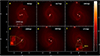 |
Fig. 4 Results of the simulation for model M4. The physical size of each individual panel is 12 667 × 12 667 au. The plots show face-on views of the column density integrated along the rotation axis(z) at 6 successive times during the evolution of the model. The color bar on the right shows log (Σ) in dimensionless units. Each calculation was performed with 250025 SPH particles. |
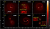 |
Fig. 5 Results of the simulation for model M5. The physical size of each individual panel is 12 667 × 12 667 au. The plots show face-on views of the column density integrated along the rotation axis(z) at 6 successive times during the evolution of the model. The color bar on the right shows log (Σ) in dimensionless units. Each calculation was performed with 250025 SPH particles. |
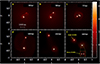 |
Fig. 6 Results of the simulation for model M6. The physical size of each individual panel is 6666 × 6666 au. The plots shows face-on views of the column density integrated along the rotation axis(z) at 6 successive times during the evolution of the model. The color bar on the right shows log (Σ) in dimensionless units. Each calculation was performed with 250025 SPH particles. |
6.4 Bursts and accretion
Figures 9 and 10 illustrate the history of the accretion rate for the individual protostellar fragments in simulations M1–M3 (Fig. 9) and M4–M6 (Fig. 10), respectively. Both Figs. 9 and 10 show that the accretion rates initially peak owing to the accretion of low-angular momentum material right at the stage of protostar formation, and then on average decrease over time, where typical average accretion rates are about 10−6 M⊙ yr−1 within a timescale of 105 yr. Even lower accretion rates seem possible at later evolutionary stages. Moreover, some sink particles are gravitationally ejected from the gas cloud so that accretion onto these protostars is suppressed. In addition to these global trends, individual peaks and short-term variations are superimposed on the long-term trend. These peaks are the hallmark of episodic accretion.
The first spike in the mass accretion profiles indicates the event of protostar formation. The first spike is then followed by a second spike, which indicates the first and sometimes only accretion burst. Protostars evolving as individual objects in our simulations show accretion burst(s) at earlier stages of the cloud collapse. For instance, in model M1, sink 6 (secondary 4), in model M2, sink 1 (primary 1) and sink 4 (secondary 2), and in model M3, sink 2 (primary 2), have undergone their first or only accretion burst after 45 kyr of molecular core evolution. The curves that show the accretion history of isolated protostars in Fig. 9 (the green line in the top left panel and the cyan line in the top right panel; the blue line in the middle left panel, and blue, green, and red lines in the middle right panel; the green line in the bottom left panel) and in Fig. 10(green linesin the top left and top right panels; the blue line in the bottom right panel) show that for the solar mass molecular cores simulated in this paper, protostars formed in isolation and represented by isolated sink particles only produce accretion bursts when these protostars are initially part of a compact system with small distances between the protostars (≤500 au) and a considerable gas reservoir available for accretion. While being part of a strongly interacting system at the initial stages of their evolution, these objects have enough material in their immediate surroundings to produce episodic accretion bursts. An illustration of this phenomenon can, for instance, be found in model M1, where the sink 2 (primary 2) never shows any sign of episodic accretion, while the isolated protostars sink 1 (primary 1) and sink 2 (primary 2) in models M2 and M3 show strong episodic accretion but only at the earlier stages of the core collapse (i.e., when the system is more compact and strongly gravitationally interacting). For example, the accretion bursts observed in sink 1 (primary 1) in model M2 cease after about 53 kyr. Sink 2 in model M3, on the other hand, continues to show accretion bursts until 90 kyr but the strength of these episodic accretion bursts keeps decreasing over time. As the collapsing cloud evolves further, these sinks become quiet and show either no or weak spikes in their mass accretion history. Furthermore, the accretion history of the sink particles included in binary systems in models M1–M4 (as shown in Table 4) suggests that episodic accretion bursts can also happen in binary systems as revealed by the spikes in their rate of mass accretion. The most important difference from isolated protostars is that for binaries episodic accretion can continue until much later stages of core collapse as illustrated by the curves for binary components in Figs. 9 and 10. In addition to the short-term accretion events that temporarily enhance the accretion rate, the longer term trends show a decline of the average accretion rate with time. There is clearly a connection with the decreasing mass in the envelope. The accretion onto the protostars can only be maintained in the presence of a sufficiently big mass reservoir. The depletion of the envelope could explain why the observed accretion luminosities of some protostars are lower than expected, if we assume that most of the accretion has already happened during the embedded phase of the protostars, which lasts for about half a million years, whereas the entire protostellar phase takes around a million years.
Another important observation from our simulations is that there does not appear to be any kind of synchronization between the accretion bursts occurring in the two components of binary systems at the earlier stages of cloud collapse. However, once these objects continue to evolve as isolated binaries within the collapsing gas, they indeed start showing precisely synchronized bursts but with a relatively weaker amplitude. This feature can be explained if these binaries end up evolving as individual systems moving through the ambient gas from one point to another; hence, these individual systems are not fed by gas that is being channeled through gravitational interactions with a nearby protostar(s). The surrounding gas acts as a uniform source of mass accretion for both components constituting a binary system that has evolved to a high mass ratio (q ≥ 0.75) by this time such as sink 1 (primary 1) and sink 3 (secondary 1) in model M1, sink 2 (primary 2) and sink 4 (secondary 2) in model M2, sink 1 (primary 1) and sink 3 (secondary 1) in model M4 as listed in Table 4. One of the binary systems formed in model M3, however, is an apparent exception to this rule. The binary composed of sink 1 (primary 1) and sink 5 (secondary 3) in this model exhibits synchronized episodic accretion bursts despite its much lower mass ratio of 0.499.
We suggest that the time of occurrence of episodic accretion for isolated protostars is controlled by how long the system hosting the individual protostar remains a dynamically compact structure. We also suggest that this mainly temporal constraint for episodic accretion is relaxed for VLM binaries. In these binary systems the non-steady accretion flow is controlled by spiral waves around the binary systems that transfer angular momentum outward and gas inward as explained by Vorobyov & Basu (2006). No such supply of material is possible for individual VLM stars evolving in isolation.
In models M2, M5, and M6, where the initial temperature of the cloud cores is increased in steps of 2 K, we observe stronger and more frequent spikes in the mass accretion rate at the later stages of evolution even for binary systems including two secondary components. Taking into account the Bondi–Hoyle accretion rate (Bondi 1952),
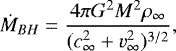 (8)
(8)
which is more relevant to the case of the disk with multiple fragments, indicates that the accretion on the (secondary-secondary) protobinary system in model M5 is not governed merely by the prevailing sound speed, which is relatively high because of the hotter core temperature compared to what we have in model M2. Despite the expected low accretion rate the (secondary-secondary) protobinary system in model M5 exhibits accretion spikes even at the later stages of the collapse. A potential explanation could be the location of this protobinary system inside the gas envelope. The local density of the gas plays a role in determining the accretion rate for the protostars (Bonnell et al. 2001). Also, Bondi–Hoyle–Lyttleton accretion becomes a more significant mechanism when the mass of the stars grows.
Our simulation results lead to the interesting conclusion that the presence of a matter-rich surrounding around individual protostars can give birth tospiral density waves that lead to accretion bursts, as described in Vorobyov & Basu (2015). There is no obvious dependence on binary parameters such as the binary mass ratio, eccentricity, total mass contained within the binary system, and core parameters such as the ratio of the envelope mass to the initial mass of cloud core as discussed in Tables 3 and 4.
Our simulations show an interesting correlation between the occurrence of episodic accretion and the mass depletion of the envelope. In the initial phase of model M1, before the envelope has lost 40 percent of its initial value in around 50 kyr, we observe much more frequent and stronger accretion bursts. Their amplitude and frequency drops down considerably as we move forward in time. So when the accretion from the envelope drops down, the amplitude and frequency of the accretion bursts also decreases significantly. However, as we increase the initial density perturbation of the cores in models M2, M3, and M4, we observe similar strong and frequent accretion bursts before the stage of 40 percent mass depletion of the envelopes in these cores, but the bursts continue to occur even after this stage has been reached. This indicates that the protostars formed in higher initial density perturbation cores have surrounding disks that remain dominant enough to support episodic mass accretion for protostars that are components of binary systems. These preliminary trends should be tested in a set of simulations exploring a larger range of initial conditions.
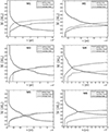 |
Fig. 7 Time evolution of the total mass contained in primary fragments (dashed lines), secondary fragments (dotted lines) as well as the remaining mass in the envelope of the core (full lines). The curves show the entire evolution for models M1–M6. The unit of mass is one solar mass and the time is expressed in years. |
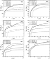 |
Fig. 8 Evolution of the mass of the individual protostellar embryos for models M1–M6. The unit of mass is solar mass and the time is in years. Each protostar corresponds to a sink particle in the simulation. Primary fragments are shown as dashed lines, while secondary fragments correspond to dotted lines, respectively. |
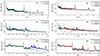 |
Fig. 9 Evolution of the mass accretion rate of the individual protostellar embryos during the evolution of models M1–M3. In model M1 the binaries are primary 1 and secondary 1 along with secondary 2 and secondary 3. In model M2 the binary is primary 2 and secondary 2. In model M3 the binaries are primary 1 and secondary 3 along with secondary 1 and secondary 2. The accretion rates for primary protostars and secondary protostars of each model are shown in the left and right panels, respectively. The accretion rate for each protostar is shown in units of log of solar mass per year. The time is indicated in years. The first spike for each appearing sink in all panels represents the formation of a protostar, which is followed by subsequent accretion bursts. |
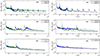 |
Fig. 10 Evolution of the mass accretion rate of the individual protostellar embryos during the evolution of models M4–M6. In model M4 the binary is primary 1 and secondary 1. In model M5 the binaries are primary 1 and primary 2 along with secondary 1 and secondary 2. In model M6 the binary is primary 1 and primary 2. The accretion rates for primary protostars and secondary protostars of each model are shown in the left and right panels, respectively. The accretion rate for each protostar is shown in units of log of solar mass per year. The time is indicated in years. The first spike for each appearing sink in all panels represents the formation of a protostar, which is followed by subsequent accretion bursts. |
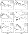 |
Fig. 11 Radial surface density profiles associated with sink 1 for models M1–M6. The extent of the radius in physical units is 120 au. |
6.5 Disk accretion
We now investigate the properties of the circumstellar disks orbiting the sink particles in more detail. In order to identify the SPH particles which are part of the disks, we require that those particles meet the first three criteria defined in Joos et al. (2012), who required that disk particles have a nearly Keplerian velocity with respect to the sinks and are part of a disk that is nearly in hydrostatic equilibrium and rotationally supported. We do not impose a threshold on the density of particles included in disks.
Figure 11 shows the azimuthally averaged radial profiles of the surface density of the gas distribution near the primary fragment sink 1 for the set of models (M1–M6). The temporal variation of the surface density profiles indicates that the disks continuously accrete matter from their surroundings. In all models (M1, M2, M3, M4, M5, M6), sink 1 is a member of a protobinary system. Choosing sink 1 to analyze the disk accretion allows us to study the behavior of protobinary disks for all initial conditions examined in this paper. We try to compare the effect of changing the initial temperatureof the cores and changing amplitudes of initial azimuthal density perturbation on the evolution of the disks.
Figure 12 shows the azimuthally averaged radial Toomre Q parameter profiles for the disks related to the primary fragment sink 1. In model M1 the Q parameter profiles suggest that the disk remains stable for most of the time but at an earlier stage of the evolution around 1.487 tff the Q parameter drops below unity in the radial range around 40 au. The drop in the Q parameter indicates the possible start of fragmentation within the disk. On the other hand, gravitational instabilities within the disk orbiting sink 1 in model M2 are far weaker. However, model M3 shows very different behavior. In model M3 the disk associated with sink 1 continues to develop gravitational instabilities for a wide range of disk radii (from 20 au to 60 au). This behavior lasts between 1.344 tff to 2.056 tff but later on the disk becomes stable as can be seen in the middle left panel of Fig. 12. Models M5 and M6 are stable against gravitational instabilities throughout their entire evolution. Model M6, however, shows an interesting feature related to the possible occurrence of gravitational instability at a much larger radius within the disk. Unlike in any other model, the disk around sink 1 in model M6 develops a gravitational instability at a much larger radius around 100 au. Later on the disk associated with the sink loses mass and regains gravitational stability.
Figure 13 represents column density plots, which illustrate the presence of spiral structures that form in the vicinity of fragments that belong to a binary or a triple system or are in the process of accreting material from their parent core as individual clumps. As we discussed previously, the spiral trail of gas around single fragments is a feature that is observed only during the earlier evolution of the system. As the collapsing molecular core evolves further in time, the spiral structures seen around single fragments gradually disappear as the disks are losing mass by accretion onto the sink and are becoming stable to gravitational fragmentation. In addition to this, it is at present difficult to establish a connection between the outbursts seen in Figs. 9 and 10 and the spiral structures seen in Fig. 13 because gravitational instabilities within single disks cannot explain the outbursts, but tidal effects by passing fragments and waves generated by orbiting binaries are a better candidate.
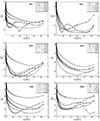 |
Fig. 12 Traces of the azimuthal average of the Toomre parameter values as a function of the radial distance in the disks associated with sink 1 for models M1–M6. The extent of the radius in physical units is 120 au. |
6.6 Binary properties
Recent observational studies of very low-mass binaries have revealed a broad range of eccentricities (0–1) associated with these systems (Dupuy & Liu 2011). The orbits of protobinaries that have been formed in our simulations via relatively later disk fragmentation (of the secondary-secondary type) tend to be more circular in our models. However, if at least one of the companions of such a system is a primary fragment that is likely formed even before the core disk structure has clearly emerged, the resulting protobinary (of the primary-secondary type) appears to have a highly elliptical orbit. This trend continues toward higher eccentricities if both components of a protobinary result from initial fragmentation (the primary-primary type) as found in model M5. However, the protobinary of the primary-primary type in model M6 remains an exception in that it appears to have a much lower value of the eccentricity and tends toward a circular orbit. Observational studies have also revealed that low-mass binaries at small separations have reduced eccentricities (Offner et al. 2010). This feature can possibly be explained as the result of tidal circularization if these binaries have been formed from fragments in a disk and continue to tidally interact with material in the disk (Offner et al. 2010). Table 4 clearly shows that our models M1, M2, M3, and M5, which have produced low-mass binaries of the secondary-secondary type, indeed have a small separation and a reduced eccentricity. Both companions in each binary are of later type fragmentation and hence they could have experienced tidal circularization. For wide binary orbits tidal circularization may be a negligible effect (Podsiadlowski et al. 2004).
Unlike the solar type population of binaries, observations reveal that there exists no correlation between eccentricity and period or semimajor axis when samples of low-mass binaries are examined (Dupuy & Liu 2011). Our simulation findings are in good agreement with these empirical results as Table 4 shows that there is no correlation of the period with the eccentricity and the semimajor axis in the simulation models that yielded low-mass binary systems. It is also interesting to note that the observed binary properties have been found to be inconsistent with previous hydrodynamic simulations (Dupuy & Liu 2011; Bate 2009) with regard to the binary eccentricities. We suggest that the model of an isolated self-gravitating solar mass core can bridge the gap between observations and theory with regard to the eccentricity of low-mass binaries. Unlike a cluster environment, an isolated solar mass molecular core gravitationally collapses to form multiple low-mass protostellar systems and a whole range of protostellar binaries with varying eccentricities as reported in the present paper. More importantly, unlike the too many highly eccentric orbits produced by the simulations reported in Stamatellos & Whitworth (2009), our models have produced binaries with a wide range of eccentricities (0.056 ≤ e ≤ 0.960), which is consistent with the results of Dupuy & Liu (2011). However, the possible impact of small number statistics means that these results are at best preliminary and more extensive simulation studies will be needed in future work.
 |
Fig. 13 Column density plots of typical spiral structures observed during the evolution of models M1, M4, and M6, respectively. The physical sizes of each respective panel are 334 229 × 317 518 au, 267 383 × 434 498 au, and 108 625 × 66 846 au. |
7 Conclusions and outlook
The simulations reported in this paper demonstrate that VLM stars can be formed as a result of both primary fragmentation and secondary fragmentation within core disks formed from collapsing solar mass molecular cloud cores. The collapsing cores form a variety of protostellar binaries and triple systems. In contrast to weakly perturbed clouds, strongly perturbed clouds produce fewer fragments within a limited range of masses. In addition, the level of the density perturbations also seems to control the delay between primary and secondary fragmentation.
We find that warmer cores produce core disks that become depleted and fall apart in circumbinary and circumstellar disks. The accumulation of mass associated with different types of fragments shows several trends. Going from small to large initial density perturbations, primary fragments are most likely to lead the mass accumulation process. However, when the cores become warmer, individual secondary fragments can eventually become more massive than the primary fragments although the total mass accumulated within these fragments remains dominant. We overall find that the accretion rates show a short peak at the time of formation, which then follows an average trend of decreasing accretion rates because of the depletion of the gas from the envelope. This average development is superimposed with peaks and short-term variations in the accretion rate, as a result of episodic accretion.
Protostars that are formed as single objects within isolated solar mass cores can exhibit accretion bursts in our models only when they are part of a matter-rich environment of a multiple system at the earlier stages of collapse. However, the possibility of burst-like accretion indeed arises even later and in isolation if a solar mass core hosts protobinary systems, but seems to be suppressed again if the cores become warmer. Despite clear evidence of the association of accretion bursts with protobinaries so far no connection has been found with the orbital elements of the binaries, hence preventing the prediction of the time of occurrence of the accretion bursts.
We find that protobinary systems consisting of (primary-primary) fragments are highly eccentric and with stronger episodic accretion. If one of the companions is of the secondary type then the eccentricity tends to get reduced. Interestingly, if protobinaries are of the secondary-secondary type, hence resulting from later disk fragmentation, the eccentricity is reduced further and the systems becomes more circular. This can likely be explained by the presence of tidal interactions with their surrounding circumbinary disks, which can lead to circularization of the system. However, if the temperature of the collapsing parent core is increased further to 12 K, even the protobinary systems of (primary-primary) type can become less eccentric (e < 0.4). As emphasized in various places, the putative trends we found in the simulations performed here should be investigated employing a larger range of realizations and initial conditions. Exploring the difference between different types of initial conditions, including turbulent gas clouds, will also be important in the future. The latter will be valuable to assess the uncertainties and spread in the model predictions, whether preliminary trends we find in this work also hold in larger samples, and whether different types of initial conditions can lead to a bias in the results.
It will also be important to explore the impact of the equation of state on the collapse dynamics and the fragmentation process. As shown by Peters et al. (2012, 2014), fragmentation occurs through the formation of self-gravitating disks if the gas temperatureincreases with density, while a decreasing temperature for increasing density leads to a filamentary fragmentation mode. The latter was shown to be relevant for instance at low metallicity, when dust grains contribute to the cooling in the primordial gas (Bovino et al. 2016). Extending the studies pursued here to different regimes may thus shed additional light on episodic accretion events, fragmentation, and the formation of filaments under different conditions.
In addition, future studies may need to explore in further detail the formation of stars within filaments. The integral shaped filament in the Orion A cloud shows strong indications for a dynamical heating of the stars, which can possibly be explained by an oscillation of the filament (Stutz & Gould 2016). The latter scenario is indeed consistent with stellar-dynamical calculations (Boekholt et al. 2017). Such filamentary structures may substantially affect the time-dependence of the accretion rate and evolution of protostars.
Acknowledgements
This research has made use of the high performance computing cluster at the Abdus Salam Centre for Physics, Pakistan and the supercomputer Leftraru, Chile. The first author (R.R.) gratefully acknowledges support from the Department of Astronomy, University of Concepcion, Chile. The first author R.R. and third author D.R.G.S. are thankful for funding through the “Concurso Proyectos Internacionales de Investigación, Convocatoria 2015” (project code PII20150171). D.R.G.S. is further thankful for funding via Fondecyt regular (project code 1161247) and via the Chilean BASAL Centro de Excelencia en Astrofísica yTecnologías Afines (CATA) grant PFB-06/2007, and ALMA-Conicyt project (proyecto code 31160001). The second author (S.V.) developed the computer code that has been used in this work on the HPC system Thinking at KU Leuven, which is part of the infrastructure of the FSC (Flemish Supercomputing Center). We thank the KU leuven support team for helping with the use of this system. The second author also gratefully acknowledges the support of Prof. Dr. Stefaan Poedts and Prof. Dr. Rony Keppens for having provided both access and funding, which made the use of the KU Leuven HPC infrastructure possible.
References
- Attwood, R.E., Goodwin, S.P., Stamatellos, D., & Whitworth, A.P. 2009, A&A, 495, 201 [NASA ADS] [CrossRef] [EDP Sciences] [Google Scholar]
- Bate, M. R. 2009, MNRAS, 392, 590 [NASA ADS] [CrossRef] [Google Scholar]
- Bate, M. R., Bonnell, I. A., & Bromm, V. 2003, MNRAS, 339, 577 [NASA ADS] [CrossRef] [Google Scholar]
- Bate, M. R., Tricco, T. S., & Price, D. J. 2014, MNRAS, 437, 77 [NASA ADS] [CrossRef] [Google Scholar]
- Boekholt, T. C., Stutz, A. M., Fellhauer, M., Schleicher, D. R., & Carrillo, D. R. M. 2017, MNRAS, 471, 3590 [NASA ADS] [CrossRef] [Google Scholar]
- Bondi, H. J. 1952, MNRAS, 112, 195 [NASA ADS] [CrossRef] [MathSciNet] [Google Scholar]
- Bonnell, I. A., Bate, M. R., Clarke, C. J., & Pringle, J. E. 2001, MNRAS, 323, 785 [NASA ADS] [CrossRef] [Google Scholar]
- Bovino, S., Grassi, T., Schleicher, D. R. G., & Banerjee, R. 2016, ApJ, 832, 154 [NASA ADS] [CrossRef] [Google Scholar]
- Burkert, A., & Bodenheimer, P. 1993, MNRAS, 264, 798 [NASA ADS] [CrossRef] [Google Scholar]
- Chen, C. C., Smail, I., Swinbank, A. M., et al. 2015, ApJ, 799, 194 [NASA ADS] [CrossRef] [Google Scholar]
- Dunham, M. M., Crapsi, A., & Evans II, N. J. 2008, ApJS, 179, 249 [NASA ADS] [CrossRef] [Google Scholar]
- Dunham, M. M., Arce, H. G., Allen, L. E., et al. 2013, ApJS, 145, 94 [Google Scholar]
- Dupuy, T. J., & Liu, M. C. 2011, ApJ, 733, 122 [NASA ADS] [CrossRef] [Google Scholar]
- Fendt, C. 2009, ApJ, 692, 346 [NASA ADS] [CrossRef] [Google Scholar]
- Federrath, C., Banerjee, R., Seifried, D., Clark, P. C., & Klessen, R. S. 2010, Proc. Int. Astron. Union, 6, 425 [CrossRef] [Google Scholar]
- Fischer, W. J., Megeath, S. T., Stutz, A. M., et al. 2013, Astron. Nachr., 334, 53 [NASA ADS] [CrossRef] [Google Scholar]
- Fischer, W. J., Megeath, S. T., Furlan, E., et al. 2017, ApJ, 840, 69 [NASA ADS] [CrossRef] [Google Scholar]
- Girichidis, P., Federrath, C., Allison, R., Banerjee, R., & Klessen, R. S. 2012, MNRAS, 420, 3264 [NASA ADS] [CrossRef] [Google Scholar]
- Goodwin, S. P., & Whitworth, A. 2007, A&A, 466, 943 [NASA ADS] [CrossRef] [EDP Sciences] [Google Scholar]
- Herbig, G. H. 1977, ApJ, 217, 693 [NASA ADS] [CrossRef] [Google Scholar]
- Hocuk, S., & Spaans, M. 2011, A&A, 536, A41 [NASA ADS] [CrossRef] [EDP Sciences] [Google Scholar]
- Hubber, D. A., Walch, S., & Whitworth, A. P. 2013, MNRAS, stt128 [Google Scholar]
- Joos, M., Hennebelle, P., & Ciardi, A. 2012, A&A, 543, A128 [NASA ADS] [CrossRef] [EDP Sciences] [Google Scholar]
- Jessop, N. E., & Ward-Thompson, D. 2001, MNRAS, 323, 1025 [NASA ADS] [CrossRef] [Google Scholar]
- Kenyon, S. J., Hartmann, L. W., Strom, K. M., & Strom, S. E. 1990, AJ, 99, 869 [NASA ADS] [CrossRef] [Google Scholar]
- Khesali, A., Nejad-Asghar, M., & Mohammadpour, M. 2013, MNRAS, 430, 961 [NASA ADS] [CrossRef] [Google Scholar]
- Kirkpatrick, J. D. 2005, ARA&A, 43, 195 [NASA ADS] [CrossRef] [Google Scholar]
- Kuffmeier, M., Frimann, S., Jensen, S. S., & Haugbølle, T. 2018, MNRAS, 475, 2642 [NASA ADS] [CrossRef] [Google Scholar]
- Law, N. M., Dhital, S., Kraus, A., Stassun, K. G., & West, A. A. 2010, ApJ, 720, 1727 [NASA ADS] [CrossRef] [Google Scholar]
- Lee, C. F. 2015, MNRAS, 374, 1347 [Google Scholar]
- Liu, M. C., Deacon, N. R., Magnier, E. A., et al. 2011, ApJ, 740, L32 [NASA ADS] [CrossRef] [Google Scholar]
- Lomax, O., Whitworth, A. P., Hubber, D. A., Stamatellos, D., & Walch, S. 2014, MNRAS, 439, 3039 [NASA ADS] [CrossRef] [Google Scholar]
- Machida, M. N., Inutsuka, S. I., & Matsumoto, T. 2010, ApJ, 724, 1006 [NASA ADS] [CrossRef] [Google Scholar]
- Megeath, S. T., Gutermuth, R., Muzerolle, J., et al. 2015, AJ, 151, 5 [Google Scholar]
- Offner, S. S., Kratter, K. M., Matzner, C. D., Krumholz, M. R., & Klein, R. I., 2010, ApJ, 725, 1485 [NASA ADS] [CrossRef] [Google Scholar]
- Peters, T., Schleicher, D. R. G., Klessen, R. S., et al. 2012, ApJ, 760, 7 [Google Scholar]
- Peters, T., Schleicher, D. R. G., Smith, R. J., Schmidt, W., & Klessen, R. S. 2014, MNRAS, 442, 3112 [NASA ADS] [CrossRef] [Google Scholar]
- Plunkett, A. L., Arce, H. G., Mardones, D., et al. 2015, Nature, 527, 70 [NASA ADS] [CrossRef] [Google Scholar]
- Podsiadlowski, P., Langer, N., Poelarends, A. J. T., et al. 2004, apj, 612, 1044 [Google Scholar]
- Price, D. J., & Monaghan, J. J. 2007, MNRAS, 374, 1347 [NASA ADS] [CrossRef] [Google Scholar]
- Reipurth, B., & Mikkola, S. 2012, Nature, 492, 221 [Google Scholar]
- Riaz, R., Farooqui, S. Z., & Vanaverbeke, S. 2014, MNRAS, 444, 1189 [NASA ADS] [CrossRef] [Google Scholar]
- Richtmyer, R. D., & Morton, K. W. 1994, Difference Methods for Initial-value Problems, 2nd ed. (Malabar, FL: Krieger Publishing Co.) [Google Scholar]
- Sigalotti, L. D. G., & Klapp, J. 2000, ApJ, 531, 1037 [NASA ADS] [CrossRef] [Google Scholar]
- Stacy, A., & Bromm, V. 2013, MNRAS, 433, 1094 [NASA ADS] [CrossRef] [Google Scholar]
- Stamatellos, D., & Whitworth, A. 2009, MNRAS, 392, 413 [Google Scholar]
- Stamatellos, D., Whitworth, A. P., & Hubber, D. A. 2012, MNRAS, 427, 1182 [NASA ADS] [CrossRef] [Google Scholar]
- Stutz, A. M., & Gould, A. 2016, A&A, 590, A2 [NASA ADS] [CrossRef] [EDP Sciences] [Google Scholar]
- Tohline, J. E. 1980, ApJ, 239, 417 [NASA ADS] [CrossRef] [Google Scholar]
- Umbreit, S., Burkert, A., Henning, T., Mikkola, S., & Spurzem, R. 2005, ApJ, 623, 940 [NASA ADS] [CrossRef] [Google Scholar]
- Vanajakshi, T. C., & Jenkins Jr, A. W. 1984, Bull. Am. Astron. Soc., 16, 526 [NASA ADS] [Google Scholar]
- Vanaverbeke, S., Keppens, R., Poedts, S., & Boffin, H. 2009, CPC, 180, 1164 [NASA ADS] [CrossRef] [Google Scholar]
- Visser, R., Bergin, E. A., & Jørgensen, J. K. 2015, A&A, 577, A102 [NASA ADS] [CrossRef] [EDP Sciences] [Google Scholar]
- Vorobyov, E. I., & Basu, S. 2006, ApJ, 650, 956 [NASA ADS] [CrossRef] [Google Scholar]
- Vorobyov, E. I., & Basu, S. 2010, ApJ, 719, 1896 [NASA ADS] [CrossRef] [Google Scholar]
- Vorobyov, E. I., & Basu, S. 2015, ApJ, 805, 115 [NASA ADS] [CrossRef] [Google Scholar]
- Walch S., Whitworth, A. P., & Girichidis, P. 2012, MNRAS, 419, 760 [NASA ADS] [CrossRef] [Google Scholar]
- Whelan, E. T., Alcalá, J. M., Bacciotti, F., et al. 2014, A&A, 570, A59 [NASA ADS] [CrossRef] [EDP Sciences] [Google Scholar]
All Tables
Summary of the initial physical parameters and the final outcome of the models discussed in this paper.
Summary of the final evolution time tf, total number of fragments Ntot, masses of the fragments (in the order as they appear in the simulation), and number of *bound* objects (VLM stars) Nbound at the end of the simulation.
Summary of the maximum evolution time in units of the initial free fall time tff, and final ratio of the envelope mass to the initial mass of cloud core for models M1–M6.
Summary of the models, type of the fragments which are components of binaries, masses of the components, mass ratio (q), semimajor axis (a), eccentricity (e), and binary separation (d) at the end of each run.
All Figures
|
Fig. 1 Results of the simulation for model M1. The physical size of each individual panel is 4333 × 4333 au. The plots show face-on views of the column density integrated along the rotation axis(z) at 6 successive times during the evolution of the model. The color bar on the right shows log (Σ) in dimensionless units. Each calculation was performed with 250025 SPH particles. |
| In the text | |
|
Fig. 2 Results of the simulation for model M2. The physical size of each individual panel is 4333 × 4333 au. The plots show face-on views of the column density integrated along the rotation axis(z) at 6 successive times during the evolution of the model. The color bar on the right shows log (Σ) in dimensionless units. Each calculation was performed with 250025 SPH particles. |
| In the text | |
|
Fig. 3 Results of the simulation for model M3. The physical size of each individual panel is 4333 × 4333 au. The plots show face-on views of the column density integrated along the rotation axis(z) at 6 successive times during the evolution of the model. The color bar on the right shows log (Σ) in dimensionless units. Each calculation was performed with 250025 SPH particles. |
| In the text | |
|
Fig. 4 Results of the simulation for model M4. The physical size of each individual panel is 12 667 × 12 667 au. The plots show face-on views of the column density integrated along the rotation axis(z) at 6 successive times during the evolution of the model. The color bar on the right shows log (Σ) in dimensionless units. Each calculation was performed with 250025 SPH particles. |
| In the text | |
|
Fig. 5 Results of the simulation for model M5. The physical size of each individual panel is 12 667 × 12 667 au. The plots show face-on views of the column density integrated along the rotation axis(z) at 6 successive times during the evolution of the model. The color bar on the right shows log (Σ) in dimensionless units. Each calculation was performed with 250025 SPH particles. |
| In the text | |
|
Fig. 6 Results of the simulation for model M6. The physical size of each individual panel is 6666 × 6666 au. The plots shows face-on views of the column density integrated along the rotation axis(z) at 6 successive times during the evolution of the model. The color bar on the right shows log (Σ) in dimensionless units. Each calculation was performed with 250025 SPH particles. |
| In the text | |
|
Fig. 7 Time evolution of the total mass contained in primary fragments (dashed lines), secondary fragments (dotted lines) as well as the remaining mass in the envelope of the core (full lines). The curves show the entire evolution for models M1–M6. The unit of mass is one solar mass and the time is expressed in years. |
| In the text | |
|
Fig. 8 Evolution of the mass of the individual protostellar embryos for models M1–M6. The unit of mass is solar mass and the time is in years. Each protostar corresponds to a sink particle in the simulation. Primary fragments are shown as dashed lines, while secondary fragments correspond to dotted lines, respectively. |
| In the text | |
|
Fig. 9 Evolution of the mass accretion rate of the individual protostellar embryos during the evolution of models M1–M3. In model M1 the binaries are primary 1 and secondary 1 along with secondary 2 and secondary 3. In model M2 the binary is primary 2 and secondary 2. In model M3 the binaries are primary 1 and secondary 3 along with secondary 1 and secondary 2. The accretion rates for primary protostars and secondary protostars of each model are shown in the left and right panels, respectively. The accretion rate for each protostar is shown in units of log of solar mass per year. The time is indicated in years. The first spike for each appearing sink in all panels represents the formation of a protostar, which is followed by subsequent accretion bursts. |
| In the text | |
|
Fig. 10 Evolution of the mass accretion rate of the individual protostellar embryos during the evolution of models M4–M6. In model M4 the binary is primary 1 and secondary 1. In model M5 the binaries are primary 1 and primary 2 along with secondary 1 and secondary 2. In model M6 the binary is primary 1 and primary 2. The accretion rates for primary protostars and secondary protostars of each model are shown in the left and right panels, respectively. The accretion rate for each protostar is shown in units of log of solar mass per year. The time is indicated in years. The first spike for each appearing sink in all panels represents the formation of a protostar, which is followed by subsequent accretion bursts. |
| In the text | |
|
Fig. 11 Radial surface density profiles associated with sink 1 for models M1–M6. The extent of the radius in physical units is 120 au. |
| In the text | |
|
Fig. 12 Traces of the azimuthal average of the Toomre parameter values as a function of the radial distance in the disks associated with sink 1 for models M1–M6. The extent of the radius in physical units is 120 au. |
| In the text | |
|
Fig. 13 Column density plots of typical spiral structures observed during the evolution of models M1, M4, and M6, respectively. The physical sizes of each respective panel are 334 229 × 317 518 au, 267 383 × 434 498 au, and 108 625 × 66 846 au. |
| In the text | |
Current usage metrics show cumulative count of Article Views (full-text article views including HTML views, PDF and ePub downloads, according to the available data) and Abstracts Views on Vision4Press platform.
Data correspond to usage on the plateform after 2015. The current usage metrics is available 48-96 hours after online publication and is updated daily on week days.
Initial download of the metrics may take a while.