| Issue |
A&A
Volume 614, June 2018
|
|
|---|---|---|
| Article Number | A46 | |
| Number of page(s) | 8 | |
| Section | Stellar structure and evolution | |
| DOI | https://doi.org/10.1051/0004-6361/201731803 | |
| Published online | 12 June 2018 | |
The envelope of the power spectra of over a thousand δ Scuti stars
The T̅eff − νmax scaling relation★
1
Departamento de Astrofísica, Centro de Astrobiología (CSIC – INTA), ESAC,
28691 Villanueva de la Cañada,
Madrid, Spain
e-mail: This email address is being protected from spambots. You need JavaScript enabled to view it.
2
Instituto de Astrofísica de Canarias,
38200
La Laguna,
Tenerife, Spain
3
Departamento de Astrofísica, Universidad de La Laguna,
38206
La Laguna,
Tenerife, Spain
4
Laboratoire AIM, CEA/DRF – CNRS – Univ. Paris Diderot – IRFU/SAp, Centre de Saclay,
91191
Gif-sur-Yvette Cedex, France
Received:
20
August
2017
Accepted:
16
February
2018
Abstract
CoRoT and Kepler high-precision photometric data allowed the detection and characterization of the oscillation parameters in stars other than the Sun. Moreover, thanks to the scaling relations, it is possible to estimate masses and radii for thousands of solar-type oscillating stars. Recently, a Δν − ρ relation has been found for δ Scuti stars. Now, analysing several hundreds of this kind of stars observed with CoRoT and Kepler, we present an empiric relation between their frequency at maximum power of their oscillation spectra and their effective temperature. Such a relation can be explained with the help of the κ-mechanism and the observed dispersion of the residuals is compatible with they being caused by the gravity-darkening effect.
Key words: asteroseismology / stars: variables: delta Scuti / stars: oscillations
Table A.1 is only available at the CDS via anonymous ftp to cdsarc.u-strasbg.fr (130.79.128.5) or via http://cdsarc.u-strasbg.fr/viz-bin/qcat?J/A+A/614/A46
© ESO 2018
1 Introduction
Our knowledge of the stellar properties is increasing as asteroseismic techniques are being developed and applied to the huge amount of data available. Ground-based telescopes and networks allowed a preliminary study of the characteristics of the oscillation modes in stars. Some of these networks, such as the Delta Scuti Network (DSN; Breger 1998) and the Stellar Photometric International network (STEPHI; Michel et al. 1995), studied δ Scuti stars with higher spectral resolution, thus improving the observing windows, and allowing the identification of several high-amplitude modes. However, the golden age for asteroseismology came with the launch of space telescopes such as CoRoT (Baglin et al. 2006) and Kepler (Borucki et al. 2010). These space missions revealed the pulsation pattern of solar-type oscillators (including red giants), thereby turning this new domain into a flourishing field.
Moreover, δ Scuti star power spectra started to be better measured and better understood (e.g. Poretti et al. 2009). This type of stars is representative of the whole intermediate-mass domain just above the domain of solar-like pulsators in terms of effective temperature (from ~6000 to ~9000 K; Uytterhoeven et al. 2011) and mass (from 1.5 to 2.5 M⊙; Breger 2000). They show from slow to fast rotation rates, as it is common in stars in this mass range and in more massive stars (Royer et al. 2007).
The oscillations of these stars are excited by the κ-mechanism (Chevalier 1971). However, turbulent pressure can also be of importance in certain peculiar cases (Antoci et al. 2014) or in δ Scuti – γ Doradus hybrids (Xiong et al. 2016). The pulsation pattern of δ Scuti stars also shows regularities, as has been assumed in several theoretical studies (e.g. Pasek et al. 2012). These regularities include the large separation, whose value is related to the mean density of the star (e.g. Suárez et al. 2014). Such a scaling relation is quite similar to the scaling relation found in solar-type oscillators (Kjeldsen & Bedding 1995) with a small deviation (from 11 to 21%). García Hernández et al. (2015) confirmed this relation by taking into account several δ Scuti stars that were observed in eclipsing binary systems, which suggests that the relation is independent of the rotation rate:
 (1)
(1)
In addition, the higher and lower limits of the pulsation pattern might be used to characterize the stars (Michel et al. 2017).
In this paper, we analyse a large sample of 1063 δ Scuti stars, observed using CoRoT and Kepler, to characterize and study the envelope of their oscillation power spectra and look for new scaling relations. In Sect. 2, we explain how we studied the envelope of the spectrum. The different results we obtained are presented in Sect. 3, including the linear relation between the frequency at maximum power, νmax, and the mean effective temperature,  , of δ Scuti stars. In Sect. 4 we further explain the observed dispersion of the measured temperature. In the final section we draw our conclusions.
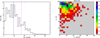 |
Fig. 1 Left panel: distribution of stars according to the number of peaks in their envelope. The mean number of peaks of the envelope (blue dashed line) is similar to the estimate made by Lignières & Georgeot (2009) for a δ Scuti star model rotating at a rate of 0.59 ΩK (purple dash-dotted line). Right panel: distribution of stars according to the number of peaks and the energy of their envelope. |
2 Data and methodology
A large sample of δ Scuti type stars is needed for a proper statistical study of their characteristics. Therefore, we have selected 1055 A and F stars with oscillations in the typical frequency range of δ Scuti type stars observed with Kepler. The Kepler Long Cadence data (LC) are sampled every ~30 min and their noise level is around 20 ppm (Koch et al. 2010). We also used the data of 8 δ Scuti stars observed with the CoRoT sismo-channel with a much shorter cadence (32 s) and a substantially higher photometric precision (between 0.6 to 4 ppm, see Auvergne et al. 2009).
Using our own methodology (δ Scuti Basics Finder; Barceló Forteza et al. 2017), we obtained the overall parameters of the oscillation modes and also characterized their power-spectral structure. Our analyses interpolate and analyse the light curve of each star with an iterative three-stage method (see Barceló Forteza et al. 2015): The first two stages allow us to interpolate the light curve using the information of the subtracted peaks. This interpolation minimizes the effect of gaps and considerably improves the background noise, thereby avoiding spurious effects (García et al. 2014). The last stage produces more accurate and precise results in terms of the parameters of the modes (frequencies, amplitudes, and phases). Furthermore, it is reasonably fast, thus making it appropriate for the study of a large sample of δ Scuti stars. Owing to the low Nyquist frequency of the LC data (283 μHz), we also made a superNyquist analysis (Murphy et al. 2013) up to 1132 μHz. This range includes all typical frequencies for δ Scuti stars (Aerts et al. 2010).
To characterize the power-spectral structure, we took into account the energy of the signal for each peak i,
 (2)
(2)
where RMSi is the root mean square of the residual signal after the extraction of highest i peaks, i = 0 for the original signal.
A number of parameters defining the envelope can be obtained; for instance, the number of peaks that form the envelope (Nenv); those that accomplish Ei ≳ 0.1% within the typical δ Scuti frequency regime, from 60 to 930 μHz (Aerts et al. 2010). The level of 0.1% is chosen since the number of peaks per energy from 0.01 to 0.1% is an order of magnitude higher than those between 0.1 to 1%. The energy of all these peaks (Eenv) compares the energy of the envelope with the energy of the entire signal. The mean amplitude of the envelope,
 (3)
(3)
where Ai is the amplitude of each peak; and the frequency at maximum power,
 (4)
(4)
where νi is the frequency of each peak. This definition is based on the weighted mean frequency used by Kallinger et al. (2010b) to measure the asymmetry of the power excess for red giants. We also measured the asymmetry of the δ Scuti stars envelopes using
 (5)
(5)
where νl and νh are the lowest and highest frequency peaks, respectively, and δνenv is its width defined as δνenv = νh − νl. We note that |α| = 0.5 is the maximum value for an asymmetric envelope.
3 Results
After we obtained their power spectra, we classified the stars in δ Scuti, γ Doradus, and hybrid stars, as explained in Uytterhoeven et al. (2011). We find that 700 of the 1055 stars (~66%) are δ Scuti stars, 225 stars (~21%) are δ Sct/γ Dor hybrids, 116 stars (~11%) are γ Dor/δ Sct hybrids, and 14 stars (~2%) are γ Doradus stars or other types of pulsators. We took into account those stars without significant pulsation in the γ Doradus regime since hybrid stars have a higher convective efficiency (Uytterhoeven et al. 2011). This is important to comply all of our assumptions (see Sect. 4.1). Only three stars are considered HADS candidates (High-Amplitude δ Scuti Stars, see Sect. 4.4). The star sample is listed in Table A.1.
3.1 Number of peaks
Figure 1 (left) shows that the power spectrum envelopes of these δ Scuti stars are formed by a few tens of peaks. The observed typical number of modes is between 5 to 45, and the mean value is 20 modes. The estimated number of 2-period island modes for a δ Scuti star model rotating at 0.59 ΩK (see Lignières & Georgeot 2009) is higher (34 ± 2 modes) but is within the typical regime. These values also agree with the number of modes found for CID 5462, CID 8669, and KIC 5892969 δ Scuti stars (Barceló Forteza et al. 2017).
The proportion of stars with a lower number of high-energy peaks might be explained in terms of a selection mechanism, such as trapping or resonances (e.g. Dziembowski 1982; Dziembowski & Krolikowska 1990). In addition, 2-period island modes show lower amplitude peaks with higher inclinations. Therefore, those 2-period island modes have amplitudes comparable to the chaotic modes for stars with inclinations close to the equator (Lignières & Georgeot 2009). As a consequence, the lower 2-period island modes could not have enough energy, Ei, to be considered as located inside the envelope. The energy of the envelope Eenv represents an 80% or higher proportion of the entire signal for most δ Scuti stars. We observed a decrease in the number of stars with high number of peaks towards lower Eenv (see Fig. 1, right). This is in agreement with the scenario described before.
We can also observe a large tail to higher number of peaks. This phenomenon can be explained by the long duration of the Kepler campaigns, which allowed us to observe the long-period cyclic variations and their associated high-amplitude sidelobes (e.g. Barceló Forteza et al. 2015). In most cases (~ 70%), these sidelobes are split from the main peak by only a few tens of nHz or less, and their characteristics are those predicted for resonance (e.g. Moskalik 1985), binarity (Shibahashi & Kurtz 2012), or aliasing (Murphy et al. 2013). The results presented in Bowman et al. (2016) agree with our observations. Then, we did not take the sidelobes of the modes into account to calculate the typical number of peaks of the envelope.
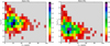 |
Fig. 2 Left panel: distribution of stars according to the number of peaks and the amplitude of their highest-amplitude mode. Rightpanel: distribution of stars according to the number of peaks and the mean amplitude of their envelope. |
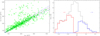 |
Fig. 3 Left panel: relation between νmax and the mean frequency of the envelope for δ Scuti stars (green triangles). The black line points to the 1:1 relation. Blue dashed lines are the limits for a significant departure from the solar case (3σ, see text). Right panel: distribution of stars according to their asymmetry (black histogram). The blue (red) histogram denotes the proportion of stars whose νmax deviation from the mean frequency of the envelope towards lower (higher) frequencies is significantly higher than the solar case (see text). |
3.2 Asymmetry
The typical amplitudes of the highest modes (A0) of δ Scuti stars are around thousands of ppm (see Fig. 2, left). However, the mean amplitude of the envelope is almost one order of magnitude lower, Aenv ~ 300 ppm (see Fig. 2, right). We also observed some cases with amplitudes up to 105 ppm and low number of modes that have been classified as HADS (see Sect. 4.4).
An interesting characteristic of the envelope is its asymmetry, which has been calculated for red giants by Kallinger et al. (2010a). They find a weak asymmetry around 3.1 ± 1.3% of the νmax value; this difference between the weighted frequency and the mean frequency of the envelope is similar to that found in the solar case. We have calculated the asymmetry of the envelope for δ Scuti stars, α (see Eq. (5)), and we observed that their envelope can be highly asymmetric, up to |α| = 0.45. Specifically, 61% of stars have a significantly higher asymmetry than the solar case (see Fig. 3) considering a higher difference than 3σ.
This asymmetry is not produced by a bias due to aliasing. The Nyquist frequency of CoRoT data is higher than the typical frequencies of δ Scuti type stars, and a superNyquist analysis (Murphy et al. 2013) has been done with Kepler data for the peaks of the envelope. There are several possible causes such as a selection mechanism (resonance, trapping; e.g. Dziembowski 1982; Dziembowski & Krolikowska 1990), and the variation of the large separation with frequency as is also seen in other types of stars (e.g. Mosser et al. 2010).
The number of stars showing asymmetry towards low-frequency modes is much higher (40%) than those that have a high-frequency asymmetry in their envelope (21%, see Fig. 3, right). This difference could be a consequence of the lower energy required to excite these lower frequency modes compared with the energy required by the higher frequency ones. Therefore, the asymmetry in the envelope may be produced by an asymmetry in the growth rate of the modes.
These statistical properties are not significantly modified by the definition of νmax. To calculate the asymmetry, we can also use the frequency of the highest amplitude mode (ν0) or the weighted mean frequency of the power spectrum instead of the amplitudes (see Eq. (4)),
 (6)
(6)
For both cases, we observed the same number of stars with asymmetric envelopes. Moreover, the same proportion of stars have an asymmetry towards low and high frequencies, although the extreme cases have higher |α|. This is in agreement with our hypothesis of the energy requirements to excite the modes.
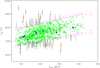 |
Fig. 4 Relation between νmax and |

3.3 Frequency at maximum power
After determining the values of νmax, we can derive the effective temperatures Teff from the input catalogues of both satellites and make a plot as shown in Fig. 4. Using only the values of Teff from the Kepler catalogue (Brown et al. 2011; Huber et al. 2014), we obtained the following linear relation (see Fig. 4):
 (7)
(7)
The observed dispersion of the data is around σ ~ 6% and the value of the Pearson correlation coefficient is R = 0.42, meaning a probability of being uncorrelated (Pu; i.e. Taylor 1997) of around
 (8)
(8)
where  is the gamma function, and N is the number of δ Scuti stars of the sample. This is the probability that N measurements of a priori two uncorrelated variables gives |R|≥ 0.42. Taking into account that a probability Pu ≤ 5% and Pu ≤ 1% mean a significant and a highly significant correlation, respectively, we found a highly significant evidence of a linear relation between the frequency at maximum power and the effective temperature. Moreover, we note that this relation is also followed by the stars observed with the CoRoT sismo-channel (see Fig. 4 blue asterisks) that have been studied in detail by several authors (e.g. Barceló Forteza et al. 2017).
We tested other possible scaling relations such as  or
or  (see Eq. (6)). Although all of them have similar slope and y-intercept values, the relation we found in Eq. (7) has the highest Pearson coefficient and lower Pu (see Table 1).
Parameters of the fitted scaling relation taking into account different definitions of the frequency at maximum power.
4 Discussion
The  scaling relation might be explained by the excitation of peaks with higher radial order with higher temperature, as was predicted by Dziembowski (1997, see Fig. 2 in their publication). Balona & Dziembowski (2011) searched for a dependence between the frequency ofthe highest amplitude and the effective temperature. The frequency they predicted for the highest growth rate seems to increase with the effective temperature (see Fig. 2 in their publication). They find that the measured values vary widely with respect to the predicted values, but the maximum value of the measured temperature increases with frequency. We observed the same effect when hybrid stars were included in our analysis, as Balona & Dziembowski (2011) did in their study.
Several possible causes might explain the observed dispersion in the scaling relation, such as the error in the temperaturemeasurements, a possible systematic error caused by the definition of the frequency at maximum power, or a physical mechanism such as the gravity-darkening effect. The relative error of the measured effective temperatures of the Kepler catalogue is about 3%, and this is not enough to explain the observations (σ ~ 6%, see Sect. 3.3). Moreover, there is a non-significant variation in the observed dispersion when we use ν0 or  instead of νmax (Δσ~ 0.05% and ~ 0.01%; see Table 1).
We might explain the dispersion with the gravity-darkening effect (von Zeipel 1924):
 (9)
(9)
where Teff(i) and geff(i) are the effective temperature and the effective gravity observed for a given inclination i, C is a constant, and the value of β depends of the evolutionary stage of the star (Claret 1998). Assuming that the surface of the star is a Roche surface (Pérez Hernández et al. 1999), the value of the effective gravity is
 (10)
(10)
where R(i) is the radius of the star for an inclination i, and Ω is its rotation. From this, the gravity-darkening effect between the equator and the poles can be obtained,
 (11)
(11)
where the values of Teff,p and Teff,e are the effective temperatures at the pole and at the equator of the stars, respectively, and
 (12)
(12)
where M is the mass, and R is the radius of a star with spherical symmetry. Moreover, the temperature difference between mid-latitudes, i ~ 55°, and any other inclination value is
 (13)
(13)
In fact,  since at that inclination the effective surface gravity is the same as that of the spherically symmetric star (Pérez Hernández et al. 1999).
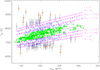 |
Fig. 5 νmax– |

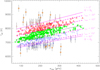 |
Fig. 6 Same as Fig. 5, but the different dashed purple lines represent the higher (lower) limits of the inclination i. Red (blue inverted) triangles represent the extremely fast δ Scuti stars observed by Kepler. |
4.1 Extremely fast rotators
The δ Scuti stars with the highest departure from the  –νmax relation should be the stars seen equator-on or pole-on whose rotation rate is close to their break-up frequency,
 (14)
(14)
where Rp is the polar radius
 (15)
(15)
Then, Eq. (12) is equivalent to
 (16)
(16)
where the maximum value possible for this dimensionless parameter is  . Taking into account that β ~ 1 for stars with fully radiative envelope (Claret 1998), the maximum temperature variation due to the gravity-darkening effect is
 (17)
(17)
Therefore, the predicted dispersion includes 98% of the stars, which suggests that the gravity-darkening effect might explain the real dispersion of the observations (see Fig. 4).
Using only the observed temperature departure,
 (18)
(18)
and Eq. (13), we can estimate the minimum value of the rotation rate (Ωmin) for each star, assuming it is pole-on or equator-on and fulfils the condition
 (19)
(19)
where ETeff is the error of the measured effective temperature (see Fig. 5). These stars (blue inverted triangles) should then be extremely fast rotators because a high rotation rate is needed to fulfil this last condition (Ω ≥ 0.7ΩK). In contrast, we can also delimit the inclination of these δ Scuti stars by assuming Ω ~ ΩK and using dTeff,obs in Eq. (13). We could find these limits for extreme rotators with inclinations i ≲ 45° or i ≳ 60° (see the red triangles and blue inverted triangles in Fig. 6, respectively). There is a degeneracy between i and Ω for those stars that do not satisfy Eq. (19) (green astersiks). Nevertheless, a deeper study of each power spectrum should allow us to distinguish a moderate or slow rotator (∀i and Ω < 0.7ΩK) from an extreme rotator with an inclination close to the mid-latitude (i ~ 55° and ∀Ω; see Barceló Forteza et al. 2017). The limits of rotation and inclination for all δ Scuti stars can also be found in Table A.1.
Measured (Col. 8) and calculated (Col. 7) effective temperature for well-known δ Scuti stars (see text).
4.2 The case of the well-known δ Scuti stars
We tested the  –νmax relation and the gravity-darkening effect using the known data of eight previously studied stars (see Table 2). We chose these δ Scuti stars because their frequency at maximum power range spans the entire region we studied. This region includes νmax higher than the Nyquist frequency of the LC Kepler light curves in order to test our results in this regime as well. In addition, this sample has stars with a wide range of inclinations (i ~25–84°) and rotation rates (Ω∕ΩK ~ 6–100%). We calculated their rotation rate using Eq. (14) and the values of mass, radius, rotation, inclination, and/or projected velocity (vsini) provided by the different authors (see Table 2).
Two of these δ Scuti stars, CID 1043 (star 1) and CID 8170 (star 6), are well-known spectroscopic binaries whose structural and orbital parameters were studied by Hareter et al. (2014) and Creevey et al. (2009), respectively. The δ Scuti star with chemical peculiarities studied by Escorza et al. (2016), CID 5685 (star 4), is a good example of the observed difference in temperature when two different methods are used. The authors use spectroscopic observations to obtain Teff= 7200 ± 80 K, quite different from that obtained with Strömgren uvbyβ photometry (Teff = 7700 ± 200 K; Poretti et al. 2005). This difference is consistent with the observations of Pinsonneault et al. (2012) who found differences of the order of 250 K between the spectroscopic and photometric methods. Another method to obtain the effective temperature is the frequency modelling. In this way, Chen et al. (2016) studied CID 123 (star 2) and found an effective temperature around Teff= 7510 ± 130 K for Z = 0.008 and Teff~ 7380 K for Z = 0.009. In the worst scenario, this result still within 1σ error for the results of Poretti et al. (2009, Teff = 7400 ± 200 K) and our paper here (see Table 2). In any case, it is preferable to compare temperature results obtained with the same method as we used to calibrate the  relation. In the case of CID 7613 (star 8), García Hernández et al. (2009) obtained a minimum rotation of around 20 μHz. To obtain Ω∕ΩK, we looked for the highest peak of the power spectrum of the subspectrum (see Fig. 3 of their publication) inside the regime
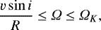 (20)
(20)
that is, ![Mathematical equation: $\frac{{{\Omega}}}{2 \pi} \in \left[20,25.8\right]$](/articles/aa/full_html/2018/06/aa31803-17/aa31803-17-eq33.png) μHz. To calculate its break-up frequency, we used Eq. (1) with Δν = 53 μHz. Based on this, the rotation rate of this star is a equal to its break-up frequency and equal to half its large separation. This is in agreement with the Ω ~ 0.94 ΩK model of a δ Scuti star calculated by Reese et al. (2017)3.
μHz. To calculate its break-up frequency, we used Eq. (1) with Δν = 53 μHz. Based on this, the rotation rate of this star is a equal to its break-up frequency and equal to half its large separation. This is in agreement with the Ω ~ 0.94 ΩK model of a δ Scuti star calculated by Reese et al. (2017)3.
When we know all the structural parameters (Ω∕ΩK, i, and Teff), we obtain the value of the calculated effective temperature (Teff(i), see Table 2) using Eq. (7) and (13). To calculate  , we only need the value of νmax, that is, the pulsation frequencies and amplitudes. These parameters of the modes are also provided by the different authors.
Finally, the value of the calculated effective temperature matches the measured effective temperature inside the 1σ error for all stars we studied (see Fig. 7 and Table 2). On the one hand, the δ Scuti stars of the CoRoT sample with low- or moderate-rotation rate (see stars 1, 2, 4, 5, and 6) do not have a significant difference in temperature owing to the inclination. Therefore, these stars allow us to suggest that the  relation is valid. On the other hand, high-rotation rate δ Scuti stars (3, 7, and 8) present a higher dependence on inclination. In these three cases, the higher inclination limit would be more appropriate to explain the observed temperature.
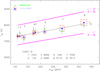 |
Fig. 7 Measured (green diamonds) and calculated (blue asterisks) effective temperature for CoRoT sismo-channel δ Scuti stars. Red and purple lines denote the |

Rotation rate limits of the outsiders.
4.3 The case of the outsiders
We found that only a 2% of the δ Scuti stars of our sample lie outside the limits of the predicted dispersion produced by the gravity-darkening effect. Most of these stars could be included if we took into account their 2 or 3σ error bars (see Fig. 4). Nevertheless, many possible physical reasons might cause a higher departure from the effective temperature of a spherically symmetric star.
One of our hypotheses was that the higher limit of the rotation rate for a stable star is Eq. (14). Considering the possibility of finding stars with a higher rotation rate, we took into account a new higher limit,
 (21)
(21)
where geff,e is the effective gravity, and
 (22)
(22)
the radius at the equator, assuming a constant volume compared with a spherically symmetric star. Therefore, the proportion of δ Scuti stars inside the predicted dispersion increases to 99.3% (see Table 3).
4.4 The case of the HADS
The High-Amplitude δ Scuti Stars should be good candidates for testing this scaling relation. These are δ Scuti stars with amplitudes around or higher than 105 ppm with temperatures between 7000 and 8000 K, approximately (McNamara 2000). Breger (2000) pointed out that most stars of this type have a slow projected velocity. In this sense, HADS seem to rotate slowly or tohave an inclination close to pole-on. As a consequence, we should find them close to the i − Ω degeneracy zone or also with higher temperatures (see KIC 2857323 and KIC 5950759 in Table 4).
In contrast, Balona et al. (2012) find that KIC 9408694 has an uncommon higher projected velocity v sin i ~ 100 km s−1. Previous studies found that only 3 of 22 have vsini > 40 km s−1 (Rodríguez et al. 2000). Balona et al. (2012) also estimated that the rotational rate is lower than Ω ≲ 15 ± 4 μHz, taking into account that the mass and the radius of the star is M ~ 2.2 ± 0.2 M⊙, and R ~ 4.5 ± 0.7 R⊙. The lowest frequency peak observed is ν ~ 34 μHz, and the authors discarded this as a rotational signal. However, we noted that half of the observed signal (~ 17 μHz) is within the limits. Using the difference in temperature due to the gravity-darkening effect, we delimited the rotation rate to Ω ≳ 0.86 ΩK and the inclination to i ≳ 76° (see Table 4). Therefore, KIC 9408694 might be an equator-on HADS showing twice the rotational frequency approximately.
We find that all three HADS of our sample are extreme rotators with a low inclination angle, except for the known special case of KIC 9408694. Therefore, our scaling relation also seems useful to characterize this type of stars. The low incidence of HADS in our sample, ~0.28%, is in agreement with the observations of other authors (Lee et al. 2008; Bowman et al. 2016).
5 Conclusions
The oscillation power spectra of 700 δ Scuti stars observed by Kepler were obtained and their overall envelope was parametrized. These envelopes could be highly asymmetric compared with low-mass stars, main-sequence stars, and red giants, especially for δ Scuti stars that have an asymmetry towards lower frequencies. This asymmetry may be produced by an asymmetry in the energy balance that is responsible for the excitation of the modes.
Furthermore, we found that the frequency at maximum power is linearly related with the mean effective temperature. This could be explained by the excitation of higher radial order modes in δ Scuti type stars with higher temperatures as predicted by Dziembowski (1997). This is an important result because knowing a power spectral characteristic we can directly obtain an intrinsic stellar parameter, independent of rotation and the point of view of the observer. The scatter of points around the fitted straight line can be explained as the gravity-darkening effect due to the oblateness of the star and its inclination with respect to the line of sight. This property allows us to delimit both rotation and inclination from the line of sight, especially for extreme rotators. The well-known δ Scuti stars observed by CoRoT sismo-channel support our findings.
Our next step is to use these delimited magnitudes to make an improved analysis of the regularities to determine the rotation and the large separation. Then, we will be able to characterize δ Scuti with a few seismic indices (Ω, Δν, νmax), as has been done for solar-type pulsators.
Rotation rate and inclination limits of the HADS candidates in our star sample.
Acknowledgements
Comments from A. Moya are gratefully acknowledged. The authors wish to thank the referee for useful suggestions that improved the paper. We also thank the CoRoT and Kepler teams whose efforts made these results possible. The CoRoT space mission has been developed and was operated by CNES, with contributions from Austria, Belgium, Brazil, ESA (RSSD and Science Program), Germany and Spain. Funding for Kepler’s Discovery mission is provided by NASA’s Science Mission Directorate. S. B. F. wishes to thank the Solar Physics team of the Universitat de les Illes Balears (UIB) for their hospitality during his stay in Majorca. He has received financial support from the grants AYA2010-20982-C02-02, ESP2015-65712-C5-1-R, and ESP2017-87676-C5-1-R. R. A. G. acknowledges the financial support from the ANR (Agence Nationale de la Recherche, France) program IDEE (n ANR-12-BS05-0008) “Interaction Des Étoiles et des Exoplanètes” and from the CNES GOLF and PLATO grants at CEA.
References
- Aerts, C., Christensen-Dalsgaard, J., & Kurtz, D. W. 2010, Asteroseismology (Berlin: Springer) [Google Scholar]
- Antoci, V., Cunha, M., Houdek, G., et al. 2014, ApJ, 796, 118 [NASA ADS] [CrossRef] [Google Scholar]
- Auvergne, M., Bodin, P., Boisnard, L., et al. 2009, A&A, 506, 411 [NASA ADS] [CrossRef] [EDP Sciences] [Google Scholar]
- Baglin, A., Auvergne, M., Barge, P., et al. 2006, ESA Spec. Publ., 1306, 33 [Google Scholar]
- Balona, L. A., & Dziembowski, W. A. 2011, MNRAS, 417, 591 [NASA ADS] [CrossRef] [Google Scholar]
- Balona, L. A., Lenz, P., Antoci, V., et al. 2012, MNRAS, 419, 3028 [NASA ADS] [CrossRef] [Google Scholar]
- Barceló Forteza, S., Michel, E., Roca Cortés, T., & García, R. A. 2015, A&A, 579, A133 [NASA ADS] [CrossRef] [EDP Sciences] [Google Scholar]
- Barceló Forteza, S., Roca Cortés, T., García Hernández, A., & García, R. A. 2017, A&A, 601, A57 [NASA ADS] [CrossRef] [EDP Sciences] [Google Scholar]
- Borucki, W. J., Koch, D., Basri, G., et al. 2010, Science, 327, 977 [NASA ADS] [CrossRef] [PubMed] [Google Scholar]
- Bowman, D. M., Kurtz, D. W., Breger, M., Murphy, S. J., & Holdsworth, D. L. 2016, MNRAS, 460, 1970 [NASA ADS] [CrossRef] [Google Scholar]
- Breger, M. 1998, in New Eyes to See Inside the Sun and Stars, eds. F.-L. Deubner, J. Christensen-Dalsgaard, & D. Kurtz, IAU Symp., 185, 323 [NASA ADS] [Google Scholar]
- Breger, M. 2000, in Delta Scuti and Related Stars, ed. M. Breger & M. Montgomery, ASP Conf. Ser., 210, 3 [NASA ADS] [Google Scholar]
- Brown, T. M., Latham, D. W., Everett, M. E., & Esquerdo, G. A. 2011, AJ, 142, 112 [NASA ADS] [CrossRef] [Google Scholar]
- Chen, X. H., Li, Y., Lai, X. J., & Wu, T. 2016, A&A, 593, A69 [NASA ADS] [CrossRef] [EDP Sciences] [Google Scholar]
- Chevalier, C. 1971, A&A, 14, 24 [NASA ADS] [Google Scholar]
- Claret, A. 1998, A&AS, 131, 395 [NASA ADS] [CrossRef] [EDP Sciences] [Google Scholar]
- Costa, J. E. S., Michel, E., Peña, J., et al. 2007, A&A, 468, 637 [NASA ADS] [CrossRef] [EDP Sciences] [Google Scholar]
- Creevey, O. L., Uytterhoeven, K., Martín-Ruiz, S., et al. 2009, A&A, 507, 901 [NASA ADS] [CrossRef] [EDP Sciences] [Google Scholar]
- Dziembowski, W. 1982, Acta Astron., 32, 147 [NASA ADS] [Google Scholar]
- Dziembowski, W. 1997, in Sounding Solar and Stellar Interiors, eds. J. Provost & F.-X. Schmider, IAU Symp., 181, 317 [NASA ADS] [Google Scholar]
- Dziembowski, W., & Krolikowska, M. 1990, Acta Astron., 40, 19 [NASA ADS] [Google Scholar]
- Escorza, A., Zwintz, K., Tkachenko, A., et al. 2016, A&A, 588, A71 [NASA ADS] [CrossRef] [EDP Sciences] [Google Scholar]
- García, R. A., Mathur, S., Pires, S., et al. 2014, A&A, 568, A10 [NASA ADS] [CrossRef] [EDP Sciences] [Google Scholar]
- García Hernández, A., Moya, A., Michel, E., et al. 2009, A&A, 506, 79 [NASA ADS] [CrossRef] [EDP Sciences] [Google Scholar]
- García Hernández, A., Moya, A., Michel, E., et al. 2013, A&A, 559, A63 [NASA ADS] [CrossRef] [EDP Sciences] [Google Scholar]
- García Hernández, A., Martín-Ruiz, S., Monteiro, M. J. P. F. G., et al. 2015, ApJ, 811, L29 [NASA ADS] [CrossRef] [Google Scholar]
- Hareter, M., Paparó, M., Weiss, W., et al. 2014, A&A, 567, A124 [NASA ADS] [CrossRef] [EDP Sciences] [Google Scholar]
- Huber, D., Silva Aguirre, V., Matthews, J. M., et al. 2014, ApJS, 211, 2 [NASA ADS] [CrossRef] [Google Scholar]
- Kallinger, T., Mosser, B., Hekker, S., et al. 2010a, A&A, 522, A1 [NASA ADS] [CrossRef] [EDP Sciences] [Google Scholar]
- Kallinger, T., Weiss, W. W., Barban, C., et al. 2010b, A&A, 509, A77 [NASA ADS] [CrossRef] [EDP Sciences] [Google Scholar]
- Kjeldsen, H., & Bedding, T. R. 1995, A&A, 293, 87 [NASA ADS] [Google Scholar]
- Koch, D. G., Borucki, W. J., Basri, G., et al. 2010, ApJ, 713, L79 [NASA ADS] [CrossRef] [Google Scholar]
- Lee, Y.-H., Kim, S. S., Shin, J., Lee, J., & Jin, H. 2008, PASJ, 60, 551 [NASA ADS] [Google Scholar]
- Lignières, F.,& Georgeot, B. 2009, A&A, 500, 1173 [NASA ADS] [CrossRef] [EDP Sciences] [Google Scholar]
- McNamara, D. H. 2000, in Delta Scuti and Related Stars, eds. M. Breger & M. Montgomery, ASP Conf. Ser., 210, 373 [NASA ADS] [Google Scholar]
- Michel, E., Chevreton, M., Goupil, M. J., et al. 1995, in Helioseismology, ESA Spec. Publ., 376, 533 [Google Scholar]
- Michel, E., Dupret, M.-A., Reese, D., et al. 2017, Eur. Phys. J. Web Conf., 160, 03001 [Google Scholar]
- Moskalik, P. 1985, Acta Astron., 35, 229 [NASA ADS] [Google Scholar]
- Mosser, B., Belkacem, K., Goupil, M.-J., et al. 2010, A&A, 517, A22 [NASA ADS] [CrossRef] [EDP Sciences] [Google Scholar]
- Murphy, S. J., Shibahashi, H., & Kurtz, D. W. 2013, MNRAS, 430, 2986 [NASA ADS] [CrossRef] [Google Scholar]
- Pasek, M., Lignières, F., Georgeot, B., & Reese, D. R. 2012, A&A, 546, A11 [NASA ADS] [CrossRef] [EDP Sciences] [Google Scholar]
- Pérez Hernández, F., Claret, A., Hernández, M. M., & Michel, E. 1999, A&A, 346, 586 [NASA ADS] [Google Scholar]
- Pinsonneault, M. H., An, D., Molenda-Żakowicz, J., et al. 2012, ApJS, 199, 30 [NASA ADS] [CrossRef] [Google Scholar]
- Poretti, E., Alonso, R., Amado, P. J., et al. 2005, AJ, 129, 2461 [NASA ADS] [CrossRef] [Google Scholar]
- Poretti, E., Michel, E., Garrido, R., et al. 2009, A&A, 506, 85 [NASA ADS] [CrossRef] [EDP Sciences] [Google Scholar]
- Reese, D. R., Lignières, F., Ballot, J., et al. 2017, A&A, 601, A130 [NASA ADS] [CrossRef] [EDP Sciences] [Google Scholar]
- Rodríguez, E., López-González, M. J., & Lopez de Coca, P. 2000, Delta Scuti Star Newsletter, 14, 12 [NASA ADS] [Google Scholar]
- Royer, F., Zorec, J., & Gómez, A. E. 2007, A&A, 463, 671 [NASA ADS] [CrossRef] [EDP Sciences] [Google Scholar]
- Shibahashi, H., & Kurtz, D. W. 2012, MNRAS, 422, 738 [NASA ADS] [CrossRef] [Google Scholar]
- Suárez, J. C., Hernández, A. G., Moya, A., et al. 2014, IAU Symp., 301, 89 [NASA ADS] [Google Scholar]
- Taylor, J. 1997, Introduction to Error Analysis, The Study of Uncertainties in Physical Measurements, 2nd edn., ed. A. McGuire (Sausalito, CA: University Science Books) [Google Scholar]
- Uytterhoeven, K., Moya, A., Grigahcène, A., et al. 2011, A&A, 534, A125 [NASA ADS] [CrossRef] [EDP Sciences] [Google Scholar]
- von Zeipel H. 1924, MNRAS, 84, 684 [NASA ADS] [CrossRef] [Google Scholar]
- Xiong, D. R., Deng, L., Zhang, C., & Wang, K. 2016, MNRAS, 457, 3163 [NASA ADS] [CrossRef] [Google Scholar]
We abbreviate the nomenclature of CoRoT ID to CID not taking into account the zeroes at the left of its identification number of ten digits.
All Tables
Parameters of the fitted scaling relation taking into account different definitions of the frequency at maximum power.
Measured (Col. 8) and calculated (Col. 7) effective temperature for well-known δ Scuti stars (see text).
All Figures
|
Fig. 1 Left panel: distribution of stars according to the number of peaks in their envelope. The mean number of peaks of the envelope (blue dashed line) is similar to the estimate made by Lignières & Georgeot (2009) for a δ Scuti star model rotating at a rate of 0.59 ΩK (purple dash-dotted line). Right panel: distribution of stars according to the number of peaks and the energy of their envelope. |
| In the text | |
|
Fig. 2 Left panel: distribution of stars according to the number of peaks and the amplitude of their highest-amplitude mode. Rightpanel: distribution of stars according to the number of peaks and the mean amplitude of their envelope. |
| In the text | |
|
Fig. 3 Left panel: relation between νmax and the mean frequency of the envelope for δ Scuti stars (green triangles). The black line points to the 1:1 relation. Blue dashed lines are the limits for a significant departure from the solar case (3σ, see text). Right panel: distribution of stars according to their asymmetry (black histogram). The blue (red) histogram denotes the proportion of stars whose νmax deviation from the mean frequency of the envelope towards lower (higher) frequencies is significantly higher than the solar case (see text). |
| In the text | |
|
Fig. 4 Relation between νmax and |
| In the text | |
|
Fig. 5 νmax– |
| In the text | |
|
Fig. 6 Same as Fig. 5, but the different dashed purple lines represent the higher (lower) limits of the inclination i. Red (blue inverted) triangles represent the extremely fast δ Scuti stars observed by Kepler. |
| In the text | |
|
Fig. 7 Measured (green diamonds) and calculated (blue asterisks) effective temperature for CoRoT sismo-channel δ Scuti stars. Red and purple lines denote the |
| In the text | |
Current usage metrics show cumulative count of Article Views (full-text article views including HTML views, PDF and ePub downloads, according to the available data) and Abstracts Views on Vision4Press platform.
Data correspond to usage on the plateform after 2015. The current usage metrics is available 48-96 hours after online publication and is updated daily on week days.
Initial download of the metrics may take a while.