| Issue |
A&A
Volume 614, June 2018
|
|
|---|---|---|
| Article Number | A4 | |
| Number of page(s) | 11 | |
| Section | The Sun | |
| DOI | https://doi.org/10.1051/0004-6361/201731343 | |
| Published online | 06 June 2018 | |
Modelling of proton acceleration in application to a ground level enhancement
1
Department of Physics and Astronomy, University of Turku,
Turku, Finland
e-mail: This email address is being protected from spambots. You need JavaScript enabled to view it.
2
Institut de Recherche en Astrophysique et Planétologie, Université de Toulouse III (UPS),
Toulouse, France
3
Centre National de la Recherche Scientifique,
UMR 5277,
Toulouse, France
4
Department of Physics, University of Helsinki,
Helsinki, Finland
5
Jeremiah Horrocks Institute, University of Central Lancashire,
Preston, UK
6
Departament de Física Quàntica i Astrofísica, Institut de Ciències del Cosmos (ICCUB), Universitat de Barcelona,
Barcelona, Spain
7
ASTRON, Netherlands Institute for Radio Astronomy,
Postbus 2,
7990 AA
Dwingeloo, The Netherlands
Received:
9
June
2017
Accepted:
22
January
2018
Abstract
Context. The source of high-energy protons (above ~500 MeV) responsible for ground level enhancements (GLEs) remains an open question in solar physics. One of the candidates is a shock wave driven by a coronal mass ejection, which is thought to accelerate particles via diffusive-shock acceleration. Aims. We perform physics-based simulations of proton acceleration using information on the shock and ambient plasma parameters derived from the observation of a real GLE event. We analyse the simulation results to find out which of the parameters are significant in controlling the acceleration efficiency and to get a better understanding of the conditions under which the shock can produce relativistic protons.
Methods. We use the results of the recently developed technique to determine the shock and ambient plasma parameters, applied to the 17 May 2012 GLE event, and carry out proton acceleration simulations with the Coronal Shock Acceleration (CSA) model.
Results. We performed proton acceleration simulations for nine individual magnetic field lines characterised by various plasma conditions. Analysis of the simulation results shows that the acceleration efficiency of the shock, i.e. its ability to accelerate particles to high energies, tends to be higher for those shock portions that are characterised by higher values of the scattering-centre compression ratio rc and/or the fast-mode Mach number MFM. At the same time, the acceleration efficiency can be strengthened by enhanced plasma density in the corresponding flux tube. The simulations show that protons can be accelerated to GLE energies in the shock portions characterised by the highest values of rc. Analysis of the delays between the flare onset and the production times of protons of 1 GV rigidity for different field lines in our simulations, and a subsequent comparison of those with the observed values indicate a possibility that quasi-perpendicular portions of the shock play the main role in producing relativistic protons.
Key words: acceleration of particles / shock waves / Sun: particle emission
© ESO 2018
1 Introduction
It has been established that enhancements in high-energy particle fluxes from the Sun, known as solar energetic particle (SEP) events, are associated with solar flares and coronal mass ejections (CMEs). Energetic particles associated with CMEs are thought to be accelerated in CME-driven shock waves by means of diffusive-shock acceleration (DSA) mechanism (e.g. Reames 2013). CME-driven shocks are also considered to be a possible source of relativistic protons responsible for ground level enhancements (GLEs; e.g. Reames 2009; Sandroos & Vainio 2009; Gopalswamy et al. 2012). For this to be possible, a shock has to exist and accelerate protons efficiently before the release time of relativistic protons from the Sun.
One of the observable signatures of a CME-driven shock in the corona is radio emission of type II detected at metre wavelengths, which is produced by shock-accelerated electrons. Reames (2009) in his study of GLE events in solar cycle 23 compared the solar particle release (SPR) times resulting from the velocity dispersion analysis of SEPs with the start times of the corresponding metric type II radio bursts. He found that all SPR times occurred after the start of metric type II bursts. Gopalswamy et al. (2012) obtained the same result using neutron monitor data to infer the relativistic proton release times. They concluded that in all of the events shocks already existed before the relativistic particle release. However, observing type II bursts is not enough to conclude that the shock is able to accelerate protons. To do that, detailed information on the shock parameters is needed.
Recently, Rouillard et al. (2016) have computed the distribution of the fast-mode Mach number over the CME-driven pressure front in the 17 May 2012 GLE event. They found that a region of increased Mach number was developing with time over the expanding front. This region evolved to a supercritical shock by the SPR time. When it becomes supercritical, a shock is able to reflect upstream ions that can be then injected to the acceleration process. This, in turn, can lead to an increase in the acceleration efficiency of the shock. For instance, in the time-dependent DSA model involving self-generated turbulence, the maximum particle energy achieved in a given time increases with the particle injection efficiency of the shock (e.g. Vainio et al. 2014; Afanasiev et al. 2015).
Thus, the result of Rouillard et al. (2016) is encouraging for the shock hypothesis of the GLE origin. However, accurate modelling of particle acceleration is needed in order to give a definitive answer. Present efforts are aimed at coupling models of particle acceleration (and transport) with realistic semi-empirical/magnetohydrodynamic (MHD) models of the CME lift-off (e.g. Kozarev et al. 2013; Kozarev & Schwadron 2016). This is important to better understand under what conditions high-energy particle production occurs and which ambient plasma and shock parameters mainly control the acceleration efficiency of the shock. In particular, Kozarev & Schwadron (2016) combined an analytic test-particle model of DSA with semi-empirical modelling ofthe evolving shock front. Their modelling shows that the most efficient particle acceleration takes place in highly oblique (quasi-perpendicular) portions of the shock. Other important parameters are the shock speed and gas compression ratio.
In this paper, we use the same approach to combine a model of DSA with a semi-empirical shock model. Our DSA model is not a test-particle model; instead, it accounts self-consistently for the formation of Alfvénic turbulent foreshock. Correspondingly, it addresses parallel and oblique shocks. We use the semi-empirical shock model obtained by Rouillard et al. (2016) for the CME-driven shock associated with the SEP/GLE event of 17 May 2012. The goals of this work are to identify which shock and plasma parameters are mainly responsible for efficient particle acceleration in oblique shocks in realistic conditions, and to try to get a better understanding of the production conditions at the shock of relativistic protons in this GLE event.
The generation of Alfvénic turbulence in coronal shocks has been addressed in a number of papers, e.g. Vainio& Laitinen (2007, 2008), Ng & Reames (2008), Afanasiev et al. (2015; see also Ng & Reames 1994 and Vainio 2003). In particular, Ng & Reames (2008) demonstrated that a fast parallel shock under typical coronal conditions is able to accelerate low-energy seed protons into a power-law energy spectrum with the cut-off energy of 300 MeV in ~10 min. However, as follows from our study, in order to resolve current uncertainties concerning GLEs it is important to conduct particle acceleration modelling for the event-specific conditions and to compare the results with the event-specific observations.
The paper is organised as follows. In Sect. 2, the numerical model used to simulate particle acceleration and the techniques used to derive the ambient plasma and shock parameters are briefly described. In Sects. 3 and 4, the simulation results and their discussion are presented. In Sect. 5, conclusions are provided.
2 Methods
2.1 Particle acceleration simulation
In this work, we employ the Coronal Shock Acceleration (CSA) code for particle acceleration simulations. It is a Monte Carlo simulation model of diffusive-shock acceleration of ions in coronal and interplanetary shocks, accounting for self-generated Alfvénic turbulence upstream of the shock. In this section, we only focus on those features of the code that are relevant for the present study. A comprehensive description of CSA can be found in Battarbee (2013); results and discussion of various aspects of the model are presented in a number of papers (Vainio & Laitinen 2007, 2008; Battarbee et al. 2011, 2013; Vainio et al. 2014; Afanasiev et al. 2015).
The CSA code simulates the coupled evolution of ions and Alfvén waves on a single radial magnetic field line. Ions are traced under the guiding-centre approximation and Alfvén waves with the Wentzel–Kramers–Brillouin (WKB) approximation complemented with a term describing diffusion in parallel wavenumber, accounting for the effect of wave–wave interactions. The wave–particle interactions are treated in the framework of quasi-linear theory (Jokipii 1966), assuming the pitch-angle-independent resonance condition. The spatial simulation domain extends from the shock front to a large distance in the shock’s upstream (usually a few hundred solar radii), i.e. the wave-particle interactions are simulated explicitly in the ambient heliospheric plasma. The effect of wave-particle interactions in the downstream is computed using a combination of test-particle simulations and calculations of the probability of return to the upstream (Jones & Ellison 1991). The shock itself is treated as a MHD discontinuity, whose gas and magnetic compression ratios are computed using the Rankine–Hugoniot relations. To compute these ratios at each time step, CSA uses analytic models of the ambient solar wind parameters (magnetic field magnitude, plasma density, solar wind speed, and temperature) and of the shock parameters (shock speed and obliquity) as functions of the heliocentric distance or the simulation time.
The model of the magnetic field implemented in CSA is given by
![Mathematical equation: \begin{equation*} B(r)=B_{0}\left(\frac{r_{\oplus}}{r}\right)^{2}\left[1+b_{f}\left(\frac{R_{\odot}}{r}\right)^{6}\right],\end{equation*}](/articles/aa/full_html/2018/06/aa31343-17/aa31343-17-eq1.png) (1)
(1)
where r is distance, R⊙ is the solar radius, r⊕ = 1 AU, and B0 and bf are the parameters that have to be specified at input. The bf parameter accounts for a super-radial expansion of the associated magnetic flux tube close to the solar surface.
The model of the plasma density is given by
 (2)
(2)
where n2, n8, and r1 are the model parameters. Here the first term accounts for the asymptotic expansion with constant solar-wind speed and the second term is the coronal component. In CSA, the solar wind speed usw (r) is computed assuming mass conservation, n(r)usw(r)∕B(r) = const, which requires the value of the solar wind speed to be specified at some distance, e.g. at 1 AU. In this work, we take usw (1 AU) = 380 km s-1.
As in some previous modelling work with CSA (e.g. Battarbee 2013), we specify the cosine of the shock-normal angle θBn as
 (3)
(3)
where μs0 and μs1 are its initial and asymptotic (at t →∞) values and q specifies its rate of change. This form allows for modelling a shock with θBn decreasing with time, which is a good approximation for many CME-driven shocks.
We also specify the shock speed along the magnetic field line as
 (4)
(4)
where V s0, t0, and γ are the model parameters.
In contrast to previous studies of particle acceleration with CSA where typical values were considered for the model parameters, in this work the model parameters in the above expressions were obtained by fitting corresponding data points computed from observations following the techniques used by Rouillard et al. (2016). Therefore, our choice of a power-law dependence for the field-aligned shock speed with the additional para- meter t0 in Eq. (4) and the inclusionof the parameter r1 in Eq. (2) were driven by better fitting results in the case of these models.
Finally, we model the plasma temperature as
 (5)
(5)
with T0 = 1.72 × 10⁶ K and α = 0.144, thus allowing a rather weak decrease with distance from the Sun. This profile is chosen ad hoc, but in the range of radial distances of interest in this study (1.5–6 R⊙), the temperature decrease is close to that resulting from the profile of Cranmer & van Ballegooijen (2005). Ions and electrons are assumed to have the same temperature and that they both contribute to the plasma pressure.
The seed particles are injected at the shock. In the injection procedure implemented in CSA (Vainio & Laitinen 2007, 2008; Battarbee et al. 2013), the speed of a given Monte Carlo seed particle is assigned by drawing it from a distribution function, which we refer to as the seed-particle pool distribution. In the version of CSA by Battarbee et al. (2013), a kappa-distribution fκ (υ) is used as the seed-particle pool distribution. It is specified by a number of parameters: the seed-particle density nseed (r) and kinetic temperature Tseed (r), which are functions of the heliocentric distance r, and the constant κ parameter, which governs the strength of the suprathermal tail. In this work, we take Tseed (r) = T(r), nseed (r) = n(r), and κ = 2 (strong suprathermal tail). Such a low value of κ is chosen to address one of the goals of this work: helping to understand whether diffusive-shock acceleration in an oblique shock is able to produce protons of GLE energies. Clearly, if our model does not produce GLE protons at κ = 2, it will not produce those at higher values of κ, i.e. for lower numbers of suprathermals in the corona. Finally, in order to exclude high-energy particles from the seed population, we have also introduced an exponential cut-off energy E0, so the seed-particle pool distribution is given by ![Mathematical equation: $f_{\mathrm{seed}}(\upsilon) = f_{\kappa}(\upsilon)\exp[-\tfrac{1}{2} m_{\mathrm{p}}\upsilon^2/E_0]$](/articles/aa/full_html/2018/06/aa31343-17/aa31343-17-eq6.png) , and take E0 = 1 MeV in all the simulations.
, and take E0 = 1 MeV in all the simulations.
2.2 Deriving shock and ambient plasma parameters
The shock and shock’s upstream plasma parameters along individual magnetic field lines are derived from the three-dimensional (3D) coronal shock modelling by Rouillard et al. (2016). Their shock fitting technique is based on the analysis of white-light and EUV images of the corona taken by the Solar and Heliospheric Observatory (SOHO), the Solar-Terrestrial Relation Observatory (STEREO), and the Solar Dynamics Observatory (SDO). The magnetic field was modelled using a potential field source surface (PFSS) extrapolation1 of the photospheric magnetograms obtained by the Helioseismic and Magnetic Imaging (HMI) instrument on board SDO.By applying the geometric fitting of the eruption images obtained from multiple vantage points, the 3D expanding shock front was triangulated, and its 3D kinematics was derived. In combination with the PFSS model, this provided the magnetic field direction and magnitude at all points on the shock surface, i.e. the 3D magnetic geometry of the shock. The white-light and EUV images were also exploited to derive the electron density in the ambient corona (Zucca et al. 2014).
An important result of Rouillard et al. (2016) is finding a spatially well-localised region crossing the expanding pressure/shock front and characterised by an elevated (fast-mode) Mach number MFM (see their Figs. 4and 5). The authors argue that this region forms just above the helmet streamer tips where the magnetic field is decreased. They associate this region with the source region of the heliospheric plasma sheet (HPS). The HPS measured in situ near 1 AU has an order of magnitude lower magnetic field and a higher plasma density than the ambient solar wind. Moreover, their analysis shows that the release of relativistic particles occurs near the time of the most significant rise in MFM.
2.3 Preparation of input for CSA simulations
We obtained the magnetic field B and plasma density n in the ambient solar wind, upstream of the shock, as well as the shock speed along field line (determined from the PFSS model) V s and the shock-normal cosine μs for 109 individual field lines, which we then fitted using the analytic functions implemented in CSA and given by Eqs. (1)–(4).
The fitting procedure for each field line started with fitting μs and V s, both as functions of time τ after the first shock-crossing of the field line. Then, using the fit of V s, the magnetic field B was fitted, i.e. to fit our 1D model given by Eq. (1) to the data, we computed the path length  along the field line and substituted r in Eq. (1) with s + (d0 + d1), where d0 is the heliocentric distance of the shock-crossing point at τ = 0 and d1 is an additional fitting parameter. So, there are actually three fitting parameters (B0, bf, and d1) to fit the magnetic field data. Finally, the plasma density n was fitted using Eq. (2) with r = s + (d0 + d1), but at this step d1 is the fitted value obtained from the magnetic field fitting.
Next, we rejected from further consideration those data sets, fitting of which gave unphysical values for the fitting parameters (17 data sets were rejected). Examples of the data sets with superposed fits for two different field lines are shown in Figs. 1 and 2. We note that for many field lines the fitting results are not perfect as the first data points lie too far from the predicted positions (e.g. Fig. 2). Nevertheless, when choosing data sets for particle acceleration simulations, we considered these cases to be acceptable. If such a case was chosen for a simulation with CSA, we started the simulation so that the shock position at the start corresponded to the second data point. In this way, we guaranteed that the plasma and shock parameters are described correctly in the simulation, but this leads to some underestimation of the acceleration.
We selected a number of field lines from among the retained ones for actual simulations with CSA (see the simulation results for further details). For the selected field lines, the values of the reduced chi-square statistic computed for each of four physical quantities, assuming the standard error of 10% of the measured value and excluding the first data point (for all field lines), are in the range  .
.
The real time corresponding to the starting time of the simulation (t = 0) for a given magnetic field is the time of intersection of that field line by the shock front or 2.5 min later in case the simulation has to be shifted as explained above (the time difference between data points is 2.5 min). Therefore, it is different for different field lines. The reference time here is the flare onset time (01:25 UT). For that reason, the corresponding initial heights of the shock front also vary from one field line to another (see Table 1).
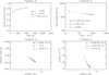 |
Fig. 1 Data points along a single field line, obtained by means of the semi-empirical shock modelling technique along with the corresponding fits by the analytic functions implemented in CSA. The top panels show the shock-normal cosine cos θBn (left) and the shock speed (right) along the field line V s, both as functions of time τ after the first shock-crossing of the field line, and the bottom panels show the magnetic field strength B (left) and the plasma density n (right), bothas functions of the radial position s + r0, where r0= d0 + d1 (see text fordetails). In each plot, the values of the corresponding fitting parameters are given as well. |
Parameters associated with the simulated magnetic field lines.
3 Simulation results
As stated above, Rouillard et al. (2016) concluded that the region of high (fast-mode) Mach number is afavourable location for strong particle acceleration. This motivated us toinvestigate the effect ofthe Mach number in our particle acceleration simulations. The Mach number is defined as MFM = V sn∕V FM,n, where V sn is the shock-normal speed and V FM,n is the fast magnetosonic wave speed along the shock normal, which is determined by the Alfvén speed, the sound speed, and the shock-normal angle (see e.g. Rouillard et al. 2016 for the exact expression).
Due to limited computing resources, we divided all the field lines pre-selected for CSA simulations into three groups according to the value of the Mach number averaged over 2000 s, which was the simulation time in all cases but one, and simulated three cases representing each group: the “weak shock” group with the average MFM ≤ 3, the “moderate shock” group with the average 3 < MFM ≤ 6, and the “strong shock” group with the average MFM > 6 (see Table 1). Figure 3 shows the plasma and shock parameters for the chosen field lines, obtained from the fitted data and plotted against simulation time (for convenience in further analysis, we show the shock-normal angle θBn instead of cos θBn and the shock-normal speed V sn instead of the field-aligned shock speed V s). The shock becomes less oblique in each case and θBn decreases faster during the first ~300 s of simulation time. Because of this (although the field-aligned shock speed V s decreases as well), the shock-normal speed V sn = V s cosθBn increases with time or has a local maximum along some field lines. The magnetic field and the density decrease monotonically with time. We note that (at least for the simulated field lines) the introduced group classification of the field lines correlates the best with the magnetic field strength rather than with the other parameters.
The evolution of the Mach number with simulation time along different field lines is shown in the left panel in Fig 4. The maximum proton energy Emax attained in each simulation is indicated for each case as well. The curves belonging to the same group of field lines are plotted with the same colour. One can see that Emax indeed tend to increase with the averaged Mach number (see also Table 1). However, this tendency may not hold for the field lines from the same group (see the green group of field lines). The right panel in Fig 4 shows the evolution of the scattering-centre compression ratio in the simulations. In CSA, the scattering-centre compression ratio is computed as 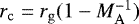 , where rg is the gas compression ratio and MA is the Alfvénic Mach number. This expression is derived under the assumption that particle scattering in the downstream region is governed by frozen-in magnetic fluctuations Vainio et al. (2014). We note a close similarity between the behaviour of rc and MFM in time.
Figure 5 shows examples of simulated energy spectra of particles and power spectra of self-generated Alfvén waves for three selected field lines, each representing a particular field line group, corresponding to three moments in time. The wave spectra are plotted against the ratio f∕fcp, where fcp is the proton cyclotron frequency. In this way, we exclude the systematic shift of the bulk of the amplified spectrum tolower frequencies, resulting from the systematic decrease in the large-scale magnetic field since fres = fcpV∕υ, and can see more clearly the effect of particle acceleration.
As expected, the simulated particle spectra have a clearly visible power-law part and a rollover. On the other hand, the spectra corresponding to different field lines evolve differently in terms of both the power-law index and the rollover. Moreover, itcan be seen that the number of high-energy particles in the spectrum for FL 27 decreases between t = 500 and 1500 s (this is also true for FL 1, although it cannot be seen from the plot). This is accompanied by a decrease in the wave energy at the resonant frequencies.
To study how acceleration efficiency of the shock evolves with time in the simulations, we use the cut-off energy Ec of the particle spectrum at the shock. It is often determined by fitting the spectrum by a function ![Mathematical equation: $CE^{-\gamma}\exp[-(E/E_{\mathrm{c}})^{\delta}]$](/articles/aa/full_html/2018/06/aa31343-17/aa31343-17-eq10.png) , where C, γ, δ, and Ec are the fitting parameters (see e.g. Afanasiev et al. 2015). There are also other methods that allow the cut-off energy to be determined more quickly but less accurately. For instance, Vainio & Laitinen (2007) defined the cut-off energy as the point of intersection between the simulated spectrum and the theoretical spectrum of Bell (1978) divided by 10. Although this method only provides an approximation for the magnitude of the actual cut-off energy (given by the fitting method), it still allows tracking dynamical changes of the spectrum in the course of a simulation. In this work, we define the cut-off energy as the point of intersection between the simulated particle spectrum at the shock and the power-law function first fitted to the simulated spectrum in the energy interval from 1 to 10 MeV and then divided by 10. In the cases where the power-law part of the spectrum clearly did not extend beyond 10 MeV (e.g. at the beginning of a simulation), we used as a cut-off energy the point of intersection between the simulated spectrum and the seed-pool particle spectrum. The left panel in Fig 6 shows the evolution of the cut-off energy in the simulations with time for different field lines. For four field lines (FLs 1, 5, 27, and 106), the cut-off energy reaches the maximum within ~ 800 s of the simulation, followed by a decrease (the most pronounced for FLs 1 and 27) and a secondary increase (FL 27). For FLs 60 and 64, the cut-off energy monotonically increases during almost the whole simulation time of 2000 s. For FL 33, there is a monotonic increase in the cut-off energy until the end of the simulation at t = 820 s. We do not show here the results for FL 25 and FL 72 as the inferred cut-off energy is ≤ 1 MeV (for FL 72, during the first half of the simulation). In fact, there are time intervals during which the scattering centre compression ratio for these field lines is ≤ 1 (see Fig. 4, right panel) and, hence, DSA does not operate. The injection of particles at those times is provided by the shock drift acceleration mechanism.
, where C, γ, δ, and Ec are the fitting parameters (see e.g. Afanasiev et al. 2015). There are also other methods that allow the cut-off energy to be determined more quickly but less accurately. For instance, Vainio & Laitinen (2007) defined the cut-off energy as the point of intersection between the simulated spectrum and the theoretical spectrum of Bell (1978) divided by 10. Although this method only provides an approximation for the magnitude of the actual cut-off energy (given by the fitting method), it still allows tracking dynamical changes of the spectrum in the course of a simulation. In this work, we define the cut-off energy as the point of intersection between the simulated particle spectrum at the shock and the power-law function first fitted to the simulated spectrum in the energy interval from 1 to 10 MeV and then divided by 10. In the cases where the power-law part of the spectrum clearly did not extend beyond 10 MeV (e.g. at the beginning of a simulation), we used as a cut-off energy the point of intersection between the simulated spectrum and the seed-pool particle spectrum. The left panel in Fig 6 shows the evolution of the cut-off energy in the simulations with time for different field lines. For four field lines (FLs 1, 5, 27, and 106), the cut-off energy reaches the maximum within ~ 800 s of the simulation, followed by a decrease (the most pronounced for FLs 1 and 27) and a secondary increase (FL 27). For FLs 60 and 64, the cut-off energy monotonically increases during almost the whole simulation time of 2000 s. For FL 33, there is a monotonic increase in the cut-off energy until the end of the simulation at t = 820 s. We do not show here the results for FL 25 and FL 72 as the inferred cut-off energy is ≤ 1 MeV (for FL 72, during the first half of the simulation). In fact, there are time intervals during which the scattering centre compression ratio for these field lines is ≤ 1 (see Fig. 4, right panel) and, hence, DSA does not operate. The injection of particles at those times is provided by the shock drift acceleration mechanism.
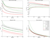 |
Fig. 3 Shock and plasma parameters resulting from fitting the data for field lines selected for CSA simulations, plotted against simulation time. The upper panels show the shock-normal angle θBn and the shock-normal speed V sn; the bottom panels show the magnetic field magnitude B and the plasma density n. The legend gives the ID number and the group type of the simulated field lines. |
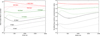 |
Fig. 4 Left panel: fast-mode Mach number of the shock versus simulation time for nine magnetic field lines for which proton acceleration simulations with CSA were performed. The black curves show the results for field lines belonging to the weakshock group of field lines, green curves to the moderate shock group, and red curves to the strong shock group (see text for details). Numbers provide the absolute maximum proton energies attained in the simulations. The total simulation time was 2000 s in all the cases except the most resource-demanding case (corresponding to red solid curve), in which it was 820 s. Right panel: scattering-centre compression ratio vs. simulation time for the corresponding field lines. |
4 Discussion
We start with discussion of the evolution of particle energy spectra in our simulations (Fig. 5). In the steady-state DSA theory of Bell, the power-law index of the spectrum ∝ E−γ is determined by the scattering-centre compression ratio rc of the shock as γ= (rc + 2)∕[2(rc − 1)] (for non-relativistic energies, e.g. Vainio et al. 2014). An increase in γ in a weakening shock explains naturally the development of a more gradual spectral rollover (as in the spectrum for FL 27 at t = 500 s in Fig. 5). In a non-steady-state situation, if the shock parameters evolve slowly, the spectral index at a given time can be expected to be approximately determined by the instantaneous value of rc. For each simulated field line, we fitted a power law to the simulated spectrum at each time and then compared the resulting spectral index with γ. We have seen that the evolution of the power-law spectral index closely follows the evolution of rc. This can also be seen from comparison of the particle energy spectra in Fig. 5 with the evolution of the scattering-centre compression ratio on the right panel in Fig 4.
We would also like to understand the temporal behaviour of the particle cut-off energy along different field lines. The decreasing cut-off energy implies that there is some energy/particle loss mechanism at work. A detailed examination of the time series of particle energy spectra shows that the implied mechanism affects mainly high-energy particles (this can also be seen in Fig. 5 for FL 27). This indicates that the wave-particle interactions alone cannot account for the cut-off energy decrease because a change d μ in the particle’s pitch-angle cosine μ due to pitch-angle scattering (as measured in the wave frame) results in a relative momentum change (as measured in the solar-fixed frame) d p∕p = (V∕v) dμ, where V = usw + V A is the phase speed of Alfvén waves and v is the particle speed, both with respect to the solar-fixed frame. Therefore, the relative momentum change due to pitch-angle scattering islarger for lower-energy particles.
The mechanism of interest can be associated with the weakening of the turbulent foreshock due to a local maximum in the Alfvén speed-radial distance profile in the corona. It was shown by Vainio (2003) that when the shock propagates towards a decreasing V A, particle trapping in the foreshock should become less efficient and the flux of escaping particles should increase. In this case, as the escaping flux has a harder spectrum than that of the trapped particles, high-energy particles can escape more efficiently, which could lead to erosion of the high-energy part of the source spectrum. Figure 7 shows the Alfvén speed plotted against simulation time for different field lines. One can see that most of the field lines have a maximum in the Alfvén speed in the time interval from 300 to 800 s. In addition, adiabatic cooling of particles, caused by the flux tube expansion and affecting particles of all energies, can also play a role.
Comparison of the Alfvén speed profiles with the simulated cut-off energy profiles (in Fig. 6) for FL 1 (dashed green line) and FL 27 (solid black line) shows that in the case of FL 1 the maximum cut-off energy is a bit delayed (t = 610 s) with respect to the maximum of the Alfvén speed (t = 580 s), whereas in the case of FL 27 it occurs somewhat earlier (at t ≈ 210 s) than the maximum of the Alfvén speed (t = 410 s). Therefore, we could expect that in the case of FL 1 the decrease in the cut-off energy is mainly caused by the weakening of the turbulent trap, and in the case of FL 27 both mechanisms are at work. FL 106 (dashed red line) experiences some reduction of the cut-off energy; FL 5 (solid green line) does as well, but it is much smaller.
In order to better understand how the acceleration process proceeds in our simulations and which plasma and shock parameters control it, we combine the steady-state DSA theory of Bell with the temporal dependence of the cut-off energy in the particle energy spectrum. This approach was used earlier by Vainio et al. (2014) to construct a time-dependentsemi-empirical model of the foreshock. We write the proton acceleration rate as
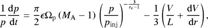 (6)
(6)
where the first term on the right-hand side results from Eq. (15) of Vainio et al. (2014) and the second term introduces the effect of adiabatic cooling into consideration. Here Ωp = eB∕mp is the proton cyclotron frequency, and it is assumed that protons being injected into the acceleration process constitute a fraction ϵ of upstream protons and the injectionoccurs at p = pinj; L =−B∕(dB∕dr) is the focusing length. One can see that the main controlling factor in the first term is the power-law factor, which is determined by the scattering-centre compression ratio. Using Bell’s solution for the particle distribution function at the shock,
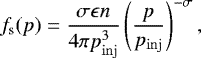 (7)
(7)
where σ = 3rc∕(rc − 1), the injection efficiency ϵ can be given as
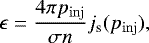 (8)
(8)
where js(pinj) is the particle intensity at the shock at p = pinj.
We integrated Eq. (6) numerically for each field line to see how well this equation describes the acceleration processes along different field lines. In the integration, for the parameters u1, n, and B, we used values extracted from the simulations. The injection efficiency ϵ was computed using Eq. (8). The parameters pinj and js(pinj) entering thisequation are governed in the simulations by the population of particles that get back to the upstream region after the first encounter with the shock. Therefore, these parameters were taken to be the momentum and intensity corresponding to the maximum of particle energy spectrum at the shock (these parameters evolve with time as well). The integration was done with the initial condition p|t=0 = pinj|t=0.
The solutions of Eq. (6) (given for energy instead of momentum) are shown in the right panel in Fig 6. By comparison with Fig. 4, we can conclude that the numerical solutions are governed mainly by the scattering-centre compression ratio rc. Furthermore, the numerical solutions reproduce the time series of Ec obtained in the simulations quite well. This indicates that rc is still the main parameter governing the particle acceleration in our simulations. However, there are also discrepancies, for example with respect to the initial increase rate and the attained maximum level (with the exception of FL 1, dashed green line, and FL 27, solid black line). These discrepancies stem from the assumption underlying Eq. (6) that the foreshock is in a fully developed steady state at any time, which implies better particle acceleration conditions than those realised in the actual simulations (see Vainio et al. 2014 for discussion on this matter). We can expect that the discrepancies should be larger for stronger shocks, which is indeed the case (cf. the scattering-centre compression ratios in Fig. 4). Furthermore, the decrease in the cut-off energy is smaller in the solutions obtained by integration. It can be seen rather well only for FL 27. This favours our suggestions that the decrease in the case of FL 1 is due to the turbulent trap weakening and in the case of FL 27 due to both adiabatic deceleration and turbulent trap weakening.
We neglect the adiabatic cooling term in Eq. (6) from now on as its contribution is small, and examine the injection efficiency ϵ and a factor Ωp(MA − 1) entering the equation for each simulated field line (see Fig. 8).
According to Battarbee et al. (2013), who carried out a detailed study of the particle injection model implemented in CSA, the injection efficiency increases with decreasing shock-normal angle θBn, especially strongly at small θBn (see e.g. their Fig. 6). We see this feature in our simulations. Specifically, FL 33 (solid red line), which takes the lowest values of θBn, reaches the highest values of ϵ, whereas FL 1 (dashed green line), which is the most oblique during the first 350 s in the simulation, has the lowest ϵ (cf. Figs. 8 and 3). In addition, there is a dependence on the shock strength given by rc or MFM (cf. Fig. 4).
Furthermore, the results of Battarbee et al. (2013) indicate that the range of θBn, where the injection efficiency strongly increases, should extend to higher values of θBn for higher values of the shock-normal speed. Namely, in their simulation for V sn = 1500 km s-1, the injection efficiency increases by two orders of magnitude for θBn decreasing from 7.5° to 0°; for V sn = 2000 km s-1 a similar increase is obtained for θBn decreasing from 15° to 0°. In our simulations, θBn changes from 24° to 10° within the whole simulation for FL 33 (within 820 s of simulation time). These values are higher than those obtained by Battarbee et al. (2013). We note, however, that in our simulations the shock corresponding to this field line is much stronger than in their study. Also, it follows from their Fig. 6 that if the shock is quite oblique (θBn > 20°), then the injection efficiency clearly decreases with increase in the shock-normal speed. Therefore, we can conclude that the shock’s strength, obliquity, and speed are all significant in controlling the injection.
In the right panel in Fig 8 we present the parameter  . One can see that FL 1 (dashed green line) is characterised by the highest values of this parameter during the first 500 s of simulation time, which is due to enhanced plasma density and high obliquity of the shock along this field line. Hence, this parameter makes a greater impact on the numerical solution of Eq. (6) for this field line (Fig. 6). Moreover, this finding explains why in the actual simulation for this field line the maximum/cut-off energy is almost as high as for FL 5 (solid green line), but is not reduced that much when compared with the corresponding numerical solution. A possible reason is that the significantly enhanced upstream plasma density provides an enhanced flux of injected particles that quickly amplifies the Alfvén wave spectrum to high intensities, comparable to the theoretical ones. We note that the particle intensity at injection energy is indeed higher for this field line than for others in the interval from ~30 to 200 s (compare also the maxima of the particle spectra along different field lines in Fig. 5 at t = 100 s). This explanation is also supported by the fact that the acceleration rate at the beginning of the simulation is not reduced much compared to the numerical solution. Thus, the upstream plasma density can strengthen the acceleration efficiency of the shock.
Figure 9 shows the Mach number distribution over the shock front at 01:45 UT together with the simulated field lines. It can be seen that the field lines belonging to the strong shock group (red lines) indeed cross the band of high Mach number. By the indicated time, according to our simulations, protons accelerated along FL 33 (solid red line) have reached the rigidity of 1 GV. This is the earliest production of relativistic protons after the flare onset, ~20 min, incomparison with the other two field lines (27.5 min for FL 106 and 31.5 min for FL 60). Of these 20 min, the acceleration process itself to 1 GV takes only ~5 min (Fig. 6) and the other 15 min is the lag between the flare onset and the time corresponding to the simulation start (Table 1). The inferred relativistic proton production time (01:45 UT) is ~5 min later than the SPR time (01:40 UT) determined by Gopalswamy et al. (2013) and ~8.6 min later than the SPR time (01:37:20 UT) inferred by Rouillard et al. (2016). We note, however, that this field line is rather far from the CME origin on the Sun as it takes ~12.5 min (after the flare onset) for the shock to reach it. There are several field lines in our total set of 109 lines, which are located closer to the CME origin, so that their first shock intersection occurs earlier (at 01:32:30 UT, the earliest available time). Those field lines are characterised by high values of the Mach number, comparable with those obtained forFL 33, starting from 01:37:30 UT (i.e. 5 min after the first intersection; we recall that the data are available at 2.5 min time resolution). Those field lines were not taken for the acceleration simulations as the quality of the parameter fitting was not good enough. Nevertheless, assuming the acceleration conditions along those field lines asfavourable as for FL 33 staring from 01:37:30 UT, we should get 1 GV protons 5 min later, i.e. at 01:42:30 UT. This is still 2.5 min later than the SPR time of Gopalswamy et al. (2013; at the error bar margin).
On the other hand, for many field lines (including FL 33) we removed the initial 2.5-min interval following the time of first intersection from the simulations (see Table 1), during which the shock is, however, weaker than at later times. So perhaps we somewhat underestimate the acceleration rate for those field lines. Also, the above analysis indicates that we need the shock and plasma parameters with better time resolution.
Therefore, it could be that the relativistic proton production in the CME-driven shock occurs at Gopalswamy et al. SPR time (01:40 UT).We recall, however, that this SPR time is obtained by using neutron monitor data and assuming the path length travelled by the particles from the source on the Sun to the Earth. On the other hand, it is rather unlikely, unless there are even more favourable conditions, that our proton acceleration model can produce 1 GV protons in this event at Rouillard et al. SPR time (01:37:20 UT), which was inferred from the velocity dispersion analysis with the use of SEP data. This may indicate that quasi-perpendicular portions of the shock play the major role in particle acceleration to relativistic energies at least in this GLE event (Sandroos & Vainio 2009). This also indicates importance of accurate determination of the SPR time.
In that connection, it is worth noting that the delays obtained for our relativistic proton productive field lines are in good correspondence with the delays obtained for 16 GLE events in cycle 23 with an average delay of 24.4 min (Gopalswamy et al. 2012). In terms of the heliocentric distances, the production of relativistic protons in our simulations occurs at rrel = 3.3 R⊙ for FL 33 and FL 106 and at rrel = 4.6 R⊙ for FL 60. These numbers are among those obtained for GLE events in cycle 23 (Reames 2009).
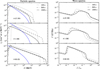 |
Fig. 5 Left panel: simulated proton energy spectra at the shock at t = 100, 500, and 1500 s for three selected field lines. The blue line in each panel shows, for reference, the spectrum of protons constituting the seed-particle pool, Iseed (E) = p2fseed(p), at t = 100 s. Right panel: corresponding simulated Alfvén wave power spectra P(f) at the shock plotted against f∕fcp, where fcp is the proton cyclotron frequency. |
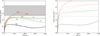 |
Fig. 6 Left panel: simulated spectral cut-off energy vs. time for different field lines. The shaded area shows the proton energy range corresponding to GLE energies. Right panel: numerical solutions of Eq. (6) for the selected field lines. |
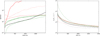 |
Fig. 8 Injection efficiency ϵ obtained with Eq. (8) (left panel) and the parameter Ωp(MA − 1) (right panel) as a function of simulation time for different field lines. |
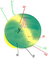 |
Fig. 9 Distribution of the Mach number over the shock front at 01:45 UT (20 min after the flare onset) crossing the simulated magnetic field lines. We note the band (light yellow) of high values of the Mach number. |
5 Conclusions
In this work, we have simulated proton diffusive-shock acceleration, using results of semi-empirical modelling of the CME-driven shock associated with the 17 May 2012 GLE event. In contrast to previous studies combining semi-empirical/MHD shock models with test-particle DSA models, we employ the Coronal Shock Acceleration simulation model, which simulates interactions of protons with Alfvén waves in the upstream region of the shock. This model allows simulations of the proton acceleration along individual magnetic field lines.
Based on the analysis of the simulations for nine magnetic field lines, we have found that the acceleration efficiency of the shock, i.e. its ability to accelerate particles to high energies, tends to be higher for those shock portions that are characterised by larger values of the scattering-centre compression ratio rc /fast-mode Mach number MFM. By comparison with Bell’s steady-state DSA theory supplemented with the temporal dependence of the spectral cut-off energy, we concluded that rc is the main shock parameter controlling the acceleration process in our simulations, but MFM is sensitive to the magnitude of rc and reveals quite closely its evolution in time. Our results, therefore, support the expectation of Rouillard et al. (2016) that most of the acceleration occurs in the region of increased Mach number. At the same time, the acceleration efficiency can be strengthened by enhanced plasma density in the corresponding flux tube. Our acceleration model also provides enhanced acceleration efficiency at shocks having small shock-normal angle θBn.
We have also found that the cut-off energy in the particle energy spectrum at the shock starts to decrease with time along some field lines. We considered two possible mechanisms leading to this effect: adiabatic cooling, which provides loss of energy for particles, and weakening of the turbulent trap due to a local maximum in the Alfvén velocity–radial distance profile, which provides loss of trapped particles. Our calculations show that the energy loss provided by the effect of adiabatic cooling alone is too small to explain the decrease in the cut-off energy. This suggests that both mechanisms may contribute with a larger contribution from the trap weakening mechanism.
Our simulations show the production of protons of GLE energies for some field lines, even though the particle acceleration efficiency of the shock in the simulations is significantly lower along those field lines than if calculated based on the DSA theory.
We have inferred the delays between the flare onset and the 1 GV proton production times for different field lines in our simulations, and compared them with the delays between the flare onset and the SPR times derived from the observations for this GLE event by Gopalswamy et al. (2013) and by Rouillard et al. (2016). If the SPR time obtained by Rouillard et al. (2016) is taken as the true one, it is rather unlikely that our model is able to explain the relativistic proton production in this event. This may indicate a possibility that quasi-perpendicular portions of the shock play the main role in producing relativistic protons.
In this paper, we focused the acceleration of SEPs during the first 20 min of a CME’s 3D expansion. In future studies, we will investigate the onset of SEP events measured over heliocentric longitudinal bands that exceed 180 degrees (e.g. Rouillard et al. 2012; Lario et al. 2017). These SEPs have been related to the lateral expansion of CMEs and their shocks propagating over extended regions of the corona. However the shock properties that control particle energisation remain unclear and our numerical model could shed new light on these events.
Acknowledgements
This project has received funding from the European Union’s Horizon 2020 research and innovation programme under grant agreement No. 637324 (HESPERIA) and from the Academy of Finland (project 267186). The computer resources of the Finnish IT Center for Science (CSC) and the FGCI project (Finland) are acknowledged. A. Aran has been partially supported by the Spanish Ministerio de Economía y Competitividad, under the project AYA2013-42614, AYA2016–77939-P and MDM-2014-0369 of ICCUB (Unidad de Excelencia “María de Maeztu”). M. Battarbee wishes to thank the Leverhulme Trust for providing funding through grant number RPG-2015-094. A.P. Rouillard acknowledges funding from the Agence Nationale de la Recherche for the COROSHOCK project (ANR-17-CE31-0006-01).
References
- Afanasiev, A., Battarbee, M., & Vainio, R. 2015, A&A, 584, A81 [NASA ADS] [CrossRef] [EDP Sciences] [Google Scholar]
- Battarbee, M. 2013, PhD Thesis, University of Turku, Finland [Google Scholar]
- Battarbee, M., Laitinen, T., & Vainio, R. 2011, A&A, 535, A34 [NASA ADS] [CrossRef] [EDP Sciences] [Google Scholar]
- Battarbee, M., Vainio, R., Laitinen, T., & Hietala, H. 2013, A&A, 558, A110 [NASA ADS] [CrossRef] [EDP Sciences] [Google Scholar]
- Bell, A. R. 1978, MNRAS, 182, 147 [NASA ADS] [CrossRef] [Google Scholar]
- Cranmer, S. R., & van Ballegooijen, A. A. 2005, ApJS, 156, 265 [NASA ADS] [CrossRef] [Google Scholar]
- Gopalswamy, N., Xie, H., Yashiro, S., et al. 2012, Space Sci. Rev., 171, 23 [NASA ADS] [CrossRef] [Google Scholar]
- Gopalswamy, N., Xie, H., Akiyama, S., et al. 2013, ApJ, 765, L30 [NASA ADS] [CrossRef] [Google Scholar]
- Jokipii, J. R. 1966, ApJ, 146, 480 [Google Scholar]
- Jones, F. C., & Ellison, D. C. 1991, Space Sci. Rev., 58, 259 [NASA ADS] [CrossRef] [Google Scholar]
- Kozarev, K. A., & Schwadron, N. A. 2016, ApJ, 831, 120 [NASA ADS] [CrossRef] [Google Scholar]
- Kozarev, K. A., Evans, R. M., Schwadron, N. A., et al. 2013, ApJ, 778, 43 [NASA ADS] [CrossRef] [Google Scholar]
- Lario, D., Kwon, R.-Y., Riley, P., & Raouafi, N. E. 2017, ApJ, 847, 103 [NASA ADS] [CrossRef] [Google Scholar]
- Ng, C. K., & Reames, D. V. 1994, ApJ, 424, 1032 [NASA ADS] [CrossRef] [Google Scholar]
- Ng, C. K., & Reames, D. V. 2008, ApJ, 686, L123 [NASA ADS] [CrossRef] [Google Scholar]
- Reames, D. V. 2009, ApJ, 693, 812 [NASA ADS] [CrossRef] [Google Scholar]
- Reames, D. V. 2013, Space Sci. Rev., 175, 53 [NASA ADS] [CrossRef] [Google Scholar]
- Rouillard, A. P., Sheeley, N. R., Tylka, A., et al. 2012, ApJ, 752, 44 [NASA ADS] [CrossRef] [Google Scholar]
- Rouillard, A. P., Plotnikov, I., Pinto, R. F., et al. 2016, ApJ, 833, 45 [NASA ADS] [CrossRef] [EDP Sciences] [Google Scholar]
- Sandroos, A., & Vainio, R. 2009, A&A, 507, L21 [CrossRef] [EDP Sciences] [Google Scholar]
- Vainio, R. 2003, A&A, 406, 735 [NASA ADS] [CrossRef] [EDP Sciences] [Google Scholar]
- Vainio, R., & Laitinen, T. 2007, ApJ, 658, 622 [NASA ADS] [CrossRef] [Google Scholar]
- Vainio, R., & Laitinen, T. 2008, J. Atm. Sol. Terr. Phys., 70, 467 [NASA ADS] [CrossRef] [Google Scholar]
- Vainio, R., Pönni, A., Battarbee, M., et al. 2014, J. Space Weather Space Clim., 4, A8 [Google Scholar]
- Zucca, P., Carley, E. P., Bloomfield, D. S., & Gallagher, P. T. 2014, A&A, 564, A47 [NASA ADS] [CrossRef] [EDP Sciences] [Google Scholar]
All Tables
All Figures
|
Fig. 1 Data points along a single field line, obtained by means of the semi-empirical shock modelling technique along with the corresponding fits by the analytic functions implemented in CSA. The top panels show the shock-normal cosine cos θBn (left) and the shock speed (right) along the field line V s, both as functions of time τ after the first shock-crossing of the field line, and the bottom panels show the magnetic field strength B (left) and the plasma density n (right), bothas functions of the radial position s + r0, where r0= d0 + d1 (see text fordetails). In each plot, the values of the corresponding fitting parameters are given as well. |
| In the text | |
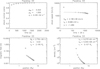 |
Fig. 2 Same as in Fig. 1, but for a different field line. |
| In the text | |
|
Fig. 3 Shock and plasma parameters resulting from fitting the data for field lines selected for CSA simulations, plotted against simulation time. The upper panels show the shock-normal angle θBn and the shock-normal speed V sn; the bottom panels show the magnetic field magnitude B and the plasma density n. The legend gives the ID number and the group type of the simulated field lines. |
| In the text | |
|
Fig. 4 Left panel: fast-mode Mach number of the shock versus simulation time for nine magnetic field lines for which proton acceleration simulations with CSA were performed. The black curves show the results for field lines belonging to the weakshock group of field lines, green curves to the moderate shock group, and red curves to the strong shock group (see text for details). Numbers provide the absolute maximum proton energies attained in the simulations. The total simulation time was 2000 s in all the cases except the most resource-demanding case (corresponding to red solid curve), in which it was 820 s. Right panel: scattering-centre compression ratio vs. simulation time for the corresponding field lines. |
| In the text | |
|
Fig. 5 Left panel: simulated proton energy spectra at the shock at t = 100, 500, and 1500 s for three selected field lines. The blue line in each panel shows, for reference, the spectrum of protons constituting the seed-particle pool, Iseed (E) = p2fseed(p), at t = 100 s. Right panel: corresponding simulated Alfvén wave power spectra P(f) at the shock plotted against f∕fcp, where fcp is the proton cyclotron frequency. |
| In the text | |
|
Fig. 6 Left panel: simulated spectral cut-off energy vs. time for different field lines. The shaded area shows the proton energy range corresponding to GLE energies. Right panel: numerical solutions of Eq. (6) for the selected field lines. |
| In the text | |
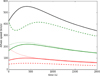 |
Fig. 7 Alfvén speed vs. simulation time for the field lines addressed in Fig. 6. |
| In the text | |
|
Fig. 8 Injection efficiency ϵ obtained with Eq. (8) (left panel) and the parameter Ωp(MA − 1) (right panel) as a function of simulation time for different field lines. |
| In the text | |
|
Fig. 9 Distribution of the Mach number over the shock front at 01:45 UT (20 min after the flare onset) crossing the simulated magnetic field lines. We note the band (light yellow) of high values of the Mach number. |
| In the text | |
Current usage metrics show cumulative count of Article Views (full-text article views including HTML views, PDF and ePub downloads, according to the available data) and Abstracts Views on Vision4Press platform.
Data correspond to usage on the plateform after 2015. The current usage metrics is available 48-96 hours after online publication and is updated daily on week days.
Initial download of the metrics may take a while.