| Issue |
A&A
Volume 614, June 2018
|
|
|---|---|---|
| Article Number | A149 | |
| Number of page(s) | 27 | |
| Section | Stellar atmospheres | |
| DOI | https://doi.org/10.1051/0004-6361/201730562 | |
| Published online | 03 July 2018 | |
Oxygen and zinc abundances in 417 Galactic bulge red giants★
1
Universidade de São Paulo, IAG,
Rua do Matão 1226, Cidade Universitária,
São Paulo
05508-900,
Brazil
e-mail: This email address is being protected from spambots. You need JavaScript enabled to view it.
2
Université de Sophia-Antipolis, Observatoire de la Côte d’Azur, CNRS UMR 6202,
BP4229,
06304
Nice Cedex 4,
France
3
Pontificia Universidad Católica de Chile, Instituto de Astrofísica,
Casilla 306,
Santiago
22,
Chile
4
Millenium Institute of Astrophysics,
Av. Vicuña Mackenna 4860, Macul,
Santiago,
Chile
5
Space Telescope Science Institute,
3700 San Martin Drive,
Baltimore,
MD
21218,
USA
6
Institute for Astronomy, University of Edinburgh, Royal Observatory,
Blackford Hill,
Edinburgh
EH9 3HJ,
UK
7
Departamento de Ciencias Físicas, Universidad Andres Bello,
República 220,
Santiago,
Chile
8
Osservatorio Astronomico di Padova,
Vicolo dell’Osservatorio 5,
35122
Padova,
Italy
9
Università di Padova, Dipartimento di Astronomia,
Vicolo dell’Osservatorio 2,
35122
Padova,
Italy
Received:
5
February
2017
Accepted:
21
February
2018
Abstract
Context. Oxygen and zinc in the Galactic bulge are key elements for the understanding of the bulge chemical evolution. Oxygen-to-iron abundance ratios provide a most robust indicator of the star formation rate and chemical evolution of the bulge. Zinc is enhanced in metal-poor stars, behaving as an α-element, and its production may require nucleosynthesis in hypernovae. Most of the neutral gas at high redshift is in damped Lyman-alpha systems (DLAs), where Zn is also observed to behave as an α-element.
Aims. The aim of this work is the derivation of the α-element oxygen, together with nitrogen, and the iron-peak element zinc abundances in 417 bulge giants, from moderate resolution (R ~ 22 000) FLAMES-GIRAFFE spectra. For stars in common with a set of UVES spectra with higher resolution (R ~ 45 000), the data are intercompared. The results are compared with literature data and chemodynamical models.
Methods. We studied the spectra obtained for a large sample of red giant stars, chosen to be one magnitude above the horizontal branch, using FLAMES-GIRAFFE on the Very Large Telescope. We computed the O abundances using the forbidden [OI] 6300.3 Å and Zn abundances using the Zn I 6362.34 Å lines. Stellar parameters for these stars were established in a previous work from our group.
Results. We present oxygen abundances for 358 stars, nitrogen abundances for 403 stars and zinc abundances were derived for 333 stars. Having oxygen abundances for this large sample adds information in particular at the moderate metallicities of −1.6 < [Fe/H] < −0.8. Zn behaves as an α-element, very similarly to O, Si, and Ca. It shows the same trend as a function of metallicity as the α-elements, i.e., a turnover around [Fe/H] ~ − 0.6, and then decreasing with increasing metallicity. The results are compared with chemodynamical evolution models of O and Zn enrichment for a classical bulge. DLAs also show an enhanced zinc-to-iron ratio, suggesting they may be enriched by hypernovae.
Key words: Galaxy: bulge – Galaxy: abundances – stars: abundances
Observations collected at the European Southern Observatory, Paranal, Chile (ESO programmes 71.B-0617A, 73.B0074A); Table B.1 is only available in electronic form at the CDS via anonymous ftp to http://cdsarc.u-strasbg.fr/ (130.79.128.5) or via http://cdsarc.u-strasbg.fr/viz-bin/qcat?J/A+A/614/A149.
© ESO 2018
1 Introduction
Oxygen and zinc are key elements for the understanding of the star formation rate and chemical enrichment of the Galactic bulge. Oxygen is the prime and most robust probe for testing the timescale of bulge formation, because it has no contribution from SNIa, and because the prescriptions from different authors (e.g. Woosley & Weaver 1995, hereafter WW95; Kobayashi et al. 2006) produce the same behaviour. Woosley et al. (2002) describe the nucleosynthesis production of the different elements. In all cases oxygen is produced in hydrostatic phases of massive star evolution.
Oxygen abundances in bulge field stars have been derived in several studies, among which the most recent are Alves-Brito et al. (2010); Bensby et al. (2013); Friaça & Barbuy (2017); Johnson et al. (2014); Jönsson et al. (2017); Meléndez et al. (2008); Rich et al. (2012); Ryde et al. (2010); Schultheis et al. (2017), and Siqueira-Mello et al. (2016). A review on abundances in the Galactic bulge is given in McWilliam (2016). A more general review on the MW bulge is presented in Barbuy et al. (2018).
Based on the observed [O/Fe] vs. [Fe/H] behaviour, as compared with their chemodynamical models, Cavichia et al. (2014), and Friaça & Barbuy (2017, hereafter FB17), derived a specific star formation rate of bulge formation and chemical enrichment of νSF ≈ 0.5 Gyr−1 or a timescale of bulge formation of 2 Gyr. The specific star formation is defined as νSF = 1∕M(M⊙)dM(M⊙)∕dt, which is the ratio of the SFR over the gas mass in M⊙ available forstar formation. A best value can be estimated from the reproduction of the observed turnover in [O/Fe] vs. [Fe/H] by the models, that occur when SNIa start to give a contribution in Fe.
Zinc is key to probe the contribution of hypernovae at the lower metallicities during the bulge chemical enrichment process. The high [Zn/Fe] ratios in bulge metal-poor stars can at present only be explained by enrichment from hypernovae (Kobayashi et al. 2006; Nomoto et al. 2013) as discussed in Barbuy et al. (2015). Zinc enhancements in metal-poor stars were derived in the literature also in halo stars by Cayrel et al. (2004); Nissen & Schuster (2011), in the thick disk by Bensby et al. (2014); Reddy et al. (2006); Mishenina et al. (2011), and in metal-poor bulge stars by Bensby et al. (2013, 2017), and Barbuy et al. (2015).
Zinc is also useful for comparisons with data from damped Lyman-alpha systems (DLAs). DLAs are neutral hydrogen gas systems observed in absorption to background quasars, with minimum hydrogen column densities of 2 × 1020 cm−2. DLAs dominate the neutral gas content at high redshift, and the metallicity in DLAs is observed to decrease with increasing redshift (Pettini et al. 1999; Rafelski et al. 2012, 2014), similar to the decrease of metallicity with age of stars in our Galaxy. Moreover, due to the neutrality of the gas, the metallicity of the gas can be measured quite precisely without ionization corrections, making them a premier site to measure abundances at high redshift. Additionally, DLAs have been found to be α-enhanced and show enhanced [Zn/Fe] ratios (Rafelski et al. 2012).
We have previously studied the oxygen and zinc abundances in the Galactic bulge based on high resolution FLAMES-UVES spectra of 56 bulge giants (Zoccali et al. 2006; Lecureur et al. 2007; Barbuy et al. 2015; FB17). In the present work we derive O and Zn abundances for 417 red giants observed with FLAMES-GIRAFFE, within the same observational programmes as the FLAMES-UVES data, at the Very Large Telescope. The stars were observed in two fields, selected among the four fields observed by Zoccali et al. (2008): Baade’s Window (BW) (l = 1.14°, b = − 4.2°), and a field at b = − 6° (l = 0.2°, b = − 6°). These stars had already been analysed by Zoccali et al. (2008), and Gonzalez et al. (2011) derived abundances of the α-elements Mg, Si, Ca, and Ti for the sample.
The sample covers a range in metallicity [Fe/H] that allows us to investigate the bulge chemical evolution history in connection to other Galactic components. It includes 65 stars with [Fe/H] ≤ − 0.5, and 14 with [Fe/H] ≤−1.0, thus covering the required range, to help impose fundamental constraints on chemical enrichment models from oxygen and zinc abundances. This is so because the bulk of the bulge stars cover the metallicity range of ~ −1.3 < [Fe/H] < ~+0.5 (Hill et al. 2011; Ness et al. 2013; Rojas-Arriagada et al. 2017; Zoccali et al. 2017), so that stars with metallicities in the range of −1.3 < [Fe/H] < −0.8 are important to understand the metal-poor end of the bulge chemical enrichment. A metal-poor end at these relatively high metallicities can be explained by the fast chemical enrichment that takes place in the bulge, rapidly reaching the metallicity of [Fe/H] ~−1.0 (e.g. Cescutti et al. 2008, and in prep.; Wise et al. 2012). In other words, the equivalent of [Fe/H] ~−3.0 in the halo, is [Fe/H] ~−1.0 in the bulge. It can also help to better constrain the interfaces between the old bulge with the inner halo, and the thick disk. Hawkins et al. (2015) suggested that moderately metal-poor stars in the bulge could define the interface of Galactic disk and inner halo, by studying stars within −1.20 < [Fe/H] < −0.55. The connection between thin and thick disks has also been studied by Mikolaitis et al. (2014).
In the present paper we have adopted the chemodynamical evolution models for an old classical bulge described in Barbuy et al. (2015) and FB17, with some modifications. In Sect. 2 the observations are summarized. In Sect. 2 the basic stellar parameters are reported, and the abundance derivation of O and Zn is described. In Sect. 2 results and discussion are presented, including comparison with literature and chemodynamical evolution models. In Sect. 6 O-poor and N-rich field stars are selected. A summary is given in Sect. 6.
2 Observations
The present data were obtained using the FLAMES-GIRAFFE instrument at the 8.2 m Kueyen of the Very Large Telescope, at the European Southern Observatory (ESO), in Paranal, Chile, as described in Zoccali et al. (2008; ESO Projects 071.B-067, 071.B-0014; PI: A. Renzini). Targets are bulge K giants, with magnitudes ~1.0 above the red clump, originally in four fields.
In the present work, we have analysed stars from two fields, reported in Table 1, among the four fields studied in Zoccali et al. (2008). These two fields were observed in setups HR13 (612.0–640.5 nm), HR14A (630.8–670.1 nm) and HR15 (660.7–696.5 nm), with resolving power respectively of R = 26 400, 18 000, and 21 350. The other two fields, NGC 6553 field at (l,b) = (5. °25, 3. °02) and Blanco field at (l,b) = (0°,12°), observed with setups HR11, HR13, and HR15, were reanalysed by Johnson et al. (2014), chosen by them because the HR11 setup contains copper lines. They derived abundances of the light elements Na, Al, α-elements O, Mg, Si and Ca, and the Fe-peak elements Cr, Fe, Co, Ni, and Cu, for 156 red giants in those fields.
Given that the same stars observed with FLAMES-UVES were also observed with FLAMES-GIRAFFE, the oxygen and zinc were derived also from the GIRAFFE spectra. The fits to both UVES and GIRAFFE spectra are shown in Appendix A for the stars in common between the two.
The sample consists of red giant branch (RGB) stars, chosen to be ~1.0 magnitude above the horizontal branch, consequently this sample does not include red clump (RC) stars, as is the case of more recent surveys (e.g. Ness et al. 2013; Rojas-Arriagada et al. 2017; Zoccali et al. 2017). Such a selection was intended to exclude brighter RGB stars in order to avoid spectra with strong TiO lines. The V, I and astrometric positions are from the OGLE catalogue (Udalski et al. 2002), a pre-FLAMES catalogue (Momany et al. 2001), and 2MASS (Carpenter, 2001), as described in Zoccali et al. (2008). The stars’ names follow the observational strategy: the targets were divided into two samples, bright and faint, in order to optimize exposure time. When a sample was being observed with GIRAFFE, the other one was observed with UVES, and then the two were swapped. The total exposure time varied from about 1 h to almost 5 h, depending on the setup and on the star luminosity, in order to ensure that the final S∕N per pixel, of each co-added spectrum to reach ~60 (see mean S∕N per field in Table 1). Therefore the identifications are Baade’s window bright (BWb) and faint (BWf), and the same for the −6 degree field with bright stars identified by B6b, and faint ones by B6f. These identifications for the UVES stars are inverted for the GIRAFFE identifications, that is, a BWb or B6b star in UVES will be a BWf or B6f in GIRAFFE, with numbers at random, corresponding to a random allocation of fibres for the observations with GIRAFFE.
Fields observed: coordinates, distance to Galactic centre, reddening as adopted in Zoccali et al. (2008), number of stars observed, and typical signal-to-noise ratios.
3 Abundance analysis
Elemental abundances were obtained through line-by-line spectrum synthesis calculations, carried out using the code described in Barbuy et al. (2003) and Coelho et al. (2005). The main molecular lines present in the region, namely the CN B2 Σ − X2Σ blue system, CN A2Π − X2Σ red system, C2 Swan A3Π − X3Π, MgH A3Π − X3Σ+, and TiO A3Φ − X3Δ γ and B3 Π − X3Δ γ’ systems were taken into account. The atmospheric models were obtained by interpolation in the grid of spherical and mildly CN-cycled ([C/Fe] = 0.13, [N/Fe] = +0.31) MARCS models by Gustafsson et al. (2008). These models consider [α/Fe] = +0.20. These models were chosen as these C and N abundances are compatible with the C, N values in normal red giants, and have suitable α-element enhancements.
We adopted the stellar parameters established by our group, given in Zoccali et al. (2006, 2008), and reported in Table B.1. A brief description of the methods follows:
-
Photometric colours [V,I] were used together with colour-temperature calibrations by Ramírez & Meléndez (2005). Another useful indicator was also used: the intensity of TiO bands. Given that RGB stars were chosen, intentionally not very bright, in order to avoid too strong TiO bands, it was possible to define a TiO band index, measuring its strength at 6190–6250 Å, for stars with Teff < 4500 K (see Zoccali et al. 2008 for further details). Effective temperatures were then checked by imposing excitation equilibrium for FeI and FeII lines of different excitation potential, using about 60 FeI lines, selected to be suitable for metallicities down to [Fe/H] ~−0.8, and another line list for more metal-poor stars.
Since the final temperatures are spectroscopic, the reddening E(B − V) and photometric temperatures were used only as initial guesses. The values of reddening reported in Table 1 are from Zoccali et al. (2006, 2008), and are compatible with the minimum values given in Schlafly & Finkbeiner (2011) in fields of 2°.1
Photometric gravities of the sample stars were obtained adopting a classical relation, where the bolometric corrections were obtained using relations by Alonso et al. (1999).
Microturbulent velocities vt were determined by imposing a constant [Fe/H] derived from FeI lines of different expected equivalent widths.
Finally, the metallicities for the sample stars were derived using a set of equivalent widths of Fe I lines.
These stellar parameters were also adopted by Gonzalez et al. (2011), for the derivation of α-element abundances.For stars in common with the UVES data, the stellar parameters derived by Zoccali et al. (2006) from FLAMES-UVES data were used.
In Zoccali et al. (2006) and Lecureur et al. (2007), the oxygen abundance for the 56 giants observed with FLAMES-UVES were derived. In Barbuy et al. (2015) these values were revisited, with the unique aim of obtaining reliable CN strengths. In FB17 the oxygen abundances in stars of this sample, observed with both UVES and GIRAFFE spectrographs, were further revised by taking into account in more detail the abundances of carbon based on the C2 (0,1) bandhead at 5635.2 Å and the C I 5380.3 Å line. These derivations replace the previous values by Zoccali et al. (2006), and Lecureur et al. (2007). A mean [C/Fe] = −0.07 ± 0.09 was found for the UVES sample. Recently, Jönsson et al. (2017) and Schultheis et al. (2017) reanalysed a fraction of the FLAMES-UVES sample.
3.1 Zinc
In Barbuy et al. (2015), we derived zinc abundances for 56 red giants observed with the FLAMES-UVES spectrograph. The Zn I 4810.53 and 6362.34 Å lines were used to derive the zinc abundances. The sample in the present work contains 23 stars observed with UVES. We revised the Zn abundances from the Zn I 4810.53 Å line observed with UVES for stars in common with the present sample. Theabundances from Barbuy et al. (2015) are reported in Table 2. In a few cases a corrected value is indicated in bold face.
In the present work, the FLAMES-GIRAFFE spectra contain the Zn I 6362.34 Å line alone. As mentioned above, in Appendix A the fits to this line with both UVES and GIRAFFE spectra are shown, for the stars common to the two samples. Literature and adopted oscillator strengths were reported, together with blending lines in Table 1 of Barbuy et al. (2015). The effect of a continuum lowering in the range ~6360.8–6363.1 Å, due to the Ca I 6361.940 autoionization line was taken into account. The continuum in the range 6361–6362 Å was the prime reference for fitting the Zn line, where the effects of the Ca I autoionization line put this region and the Zn I line at the same continuum level. The FWHM of lines was fitted for each star for a region around the Zn I line.
The Zn I 6362.339 Å line is sometimes blended with CN lines, as extensively discussed in Barbuy et al. (2015). For this reason, it is necessary to have a suitable derivation of C, N, and O abundances. In the present work we have derived Zn abundances for 333 stars among the 417 sample ones, where the line was well defined.
Sample of stars observed with both FLAMES-UVES and FLAMES-GIRAFFE.
3.2 Carbon, nitrogen, and oxygen abundances
The derivation of C, N, and O abundances proceeded as described below.
Carbon: since the present spectra have neither the Swan C2 (0,1) A3 Π − X3Π bandhead at 5635 Å, nor the C I 5380.3 Å line, and in the absence of a reliable C abundance indicator, we adopted a value of [C/Fe] = −0.2 for all stars, a deficiency expected in red giants (e.g. Smiljanic et al. 2009), compatible with the mean [C/Fe] = −0.07 found for the UVES sample, see FB17, their Table A.1. For stars that are also observed with UVES, as well as with Zoccali et al. (2006); Barbuy et al. (2015), and FB17, the UVES results are preferred. The effect of C abundance in the O abundance is illustrated in Barbuy (1988, their Fig. 2). The N abundance, as derived from a CN bandhead depends on the C abundance adopted. Despite an uncertainty on the N abundance due to this assumption, we remind the reader that the main aim here is to be able to reproduce the CN line intensities, given the blend with CN lines on the right wing of the Zn I 6362.339 Å line.
Nitrogen: we used the red CN (5,1) A2Π − X2Σ bandhead at 6332.18 Å, to derive N abundances, adopting the laboratory line list by Davis & Phillips (1963). Nitrogen abundances are important for the dissociative equilibrium between C, N, and O (e.g. Tsuji 1973; Irwin 1988). In red giants N abundances are more informative on the CN-cycle than on chemical evolution. This is due to the transformation of C into N due to the CNO-cycle that takes place along the ascent of the giant branch. Added to the expected mixing process, there is an observed extra-mixing (see e.g. Smiljanic et al. 2009). Therefore the enhanced N abundances observed are due to stellar evolution processes, and do not reflect necessarily the N abundance of the gas from which the star formed. The very few cases of very high nitrogen abundances, combined with low oxygen abundances, are discussed in Sect. 6.
Oxygen: the forbidden oxygen [OI]6300.311 Å line was used to derive O abundances, adopting log gf = −9.716, and taking into account the blends with Ni I lines at 6300.300 and 6300.350 Å, where we adopted Ni abundances varying in lockstep with Fe, as expected (e.g. Bensby et al. 2014, 2017). A solar abundance of A(O) = 8.76 is adopted (Steffen et al. 2015).
In conclusion, the abundances of N, O and Zn were derived iteratively in this order. The CN line intensity that appears as an asymmetry on the right wing of the Zn I 6362 Å line, is also used to check the N and O abundances.
Table B.1 gives the atmospheric parameters adopted from Zoccali et al. (2008), and the resulting N, O, and Zn abundances for 417 stars in Baade’s window and the −6 degree fields. In Table 2 are presented the abundances derived for N, O, and Zn for the 23 sample stars having FLAMES-UVES spectra. The Zn abundances from the ZnI 4810 Å line were revised, and slightly modified in a few cases (indicated in bold face). For deriving the present N, O, and Zn abundances for these stars, we adopted the parameters from the UVES analysis (Zoccali et al. 2006; Lecureur et al. 2007). As explained above (Sect. 3), the C, N, and O abundances reported first in Zoccali et al. (2006) and Lecureur et al. (2007), were partially revised in Barbuy et al. (2015), and the revision was further completed by FB17, and these latter are the values adopted here.
In Table 3 we report the stellar parameters and N, O, and Zn abundances for the 23 stars from both UVES and GIRAFFE data. In Fig. 1 we compare the abundances of O, N, and Zn derived from the GIRAFFE data with those derived from the UVES spectra. The oxygen abundances are in very good agreement. Nitrogen abundances appear somewhat higher in GIRAFFE spectra with respect to those in UVES. For N we could not refit C, since we have no atomic or molecular line for this element, and this may be the source of the discrepancy. Zinc tends to be lower in GIRAFFE spectra than in the UVES ones; in Fig. 1 the difference is larger for the UVES values given for the mean of abundances derived from the two lines Zn I 4810.5 and 6362.3 Å, and less discrepant when comparing results for the same line as in the GIRAFFE spectra.
Sample of 23 stars observed with both FLAMES-UVES, and FLAMES-GIRAFFE for comparison purposes.
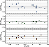 |
Fig. 1 Comparison between GIRAFFE and UVES abundances for O, N, and Zn for the stars common to the two sets of spectra (Table 3). For Zn: orange full circles consider the mean of two lines in the UVES results, and violet full triangles compare results for the same line. |
3.3 Errors
For stars in common with UVES, we adopted the same uncertainties given in Barbuy et al. (2013), amounting to Teff ± 150 K for effective temperature, log g ± 0.20 for surface gravity, [Fe/H] ± 0.10 in metallicity, and vt ± 0.10 km s−1 for microturbulent velocity. For the stars that have only GIRAFFE spectra we adopted higher uncertainties, due to having a lower resolution in the measurements of Fe I and Fe II lines, of ±200 K for Teff, ±0.40 for log g, ±0.10 in [Fe/H] and ±0.30 km s−1 for microturbulent velocity.
The errors in [O/Fe] and [Zn/Fe] are computed by using model atmospheres with parameters changed by these uncertainties, applied to the representative stars: the cooler star BW-b6, and the hotter star B6-b3. Both of these were also analysed by Jönsson et al. (2017), as shown in Table 5.
These uncertainties are given in Table 4. Since the stellar parameters are covariant, the sum of these errors is an upper limit. On the other hand, a continuum location uncertainty introduces a further uncertainty in [O/Fe] ~±0.05 and [Zn/Fe] ~±0.05.
Uncertainties on the derived [O/Fe] and [Zn/Fe] values for model changes of Δ Teff = 150, 200 K, Δ log g = + 0.2, 0.4, Δ vt = +0.1, 0.2, 0.3 km s−1, for UVES and GIRAFFE data respectively, and corresponding total error, applied to the stellar parameters Teff, log g, [Fe/H], vt of stars BW-b6 (4200 K, 1.7, −0.25, 1.3 km s−1), and B6-b3 (4700 K, 2.0, 0.10, 1.6 km s−1).
Sample of stars observed with both FLAMES-UVES, and reanalysed by Jönsson et al. (2017).
4 Results
Table B.1 reports the stellar parameters by Zoccali et al. (2008) for the GIRAFFE sample. For stars for which we have both UVES and GIRAFFE spectra, the two sets of parameters and results are reported in Table B.1, with the UVES ones first, marked with a star (*), and the GIRAFFE ones just below. In this Table are given the OGLE, GIRAFFE and UVES names, stellar parameters, the derived N, O and Zn abundances, and the α-elements Mg, Si, Ca, and Ti analysed by Gonzalez et al. (2011).
4.1 Oxygen abundances
In FB17 we discussed the available previous work on bulge samples with reported derivations of oxygen abundances. These were the bulge dwarfs by Bensby et al. (2013), the red giant stars from Alves-Brito et al. (2010) that were carried out in the optical for the samestars as in Meléndez et al. (2008); Cunha & Smith (2006); Ryde et al. (2010); Rich et al. (2012); Johnson et al. (2014); Rich and Origlia (2005) and Fulbright et al. (2007).
We now compare the present oxygen abundances for the GIRAFFE sample together with those from the UVES sample, given in FB17, compared with: (a) the reanalysis of stellar parameters carried out by Jönsson et al. (2017) for 23 stars of the same UVES data, for which they derived oxygen abundances, except for one of them (B3-f1) that FB17 did not include in their study; (b) Ryde et al. (2010) where five stars of our UVES sample were included, plus another six stars; (c) recent results by Schultheis et al. (2017), where comparisons with a fraction of the present stars were given; (d) recent results for microlensed dwarf stars by Bensby et al. (2017).
Figure 3 shows the [O/Fe] vs. [Fe/H] for the present sample (excluding six N-rich, O-poor stars), plotted together with oxygen abundances from UVES data for stars in common, analysed both by FB17, and Jönsson et al. (2017), as well as Ryde et al. (2010); Schultheis et al. (2017), and Bensby et al. (2017). Also included are recent oxygen abundances for metal-poor stars located in outer bulge fields: five stars from García-Pérez et al. (2013), two stars from Howes et al. (2016), and three stars from Lamb et al. (2017).
In Figs. 3 and 4 we overplot the behaviour of oxygen and zinc respectively, in chemodynamical models representing a classical bulge, as described in FB17, and briefly summarized as follows. The evolution of the model was followed up to 13 Gyr, and although the bulge is formed rapidly the star formation goes on, and the stellar mass is built up during at least ≈3 Gyr, allowing for a contribution from type Ia supernovae (SNIa). The best fit model for oxygen, based on previous data, was assumed to have a specific star formation rate of νSF = 0.5 Gyr−1, following conclusions by FB17, and Cavichia et al. (2014).
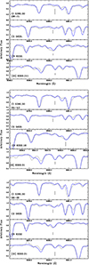 |
Fig. 2 CNO abundances rederived for stars BW-f1 B6-b3, B6-f8, adopting stellar parameters defined by Jönsson et al. (2017). Symbols: black dotted line: observed spectra; blue solid line: synthetic spectra. |
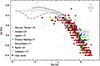 |
Fig. 3 [O/Fe] vs. [Fe/H] for 351 red giants (excluding N-rich, O-poor ones). Chemodynamical evolution models from FB17 with formation timescale of 2 Gyr, or specific star formation rate of 0.5 Gyr−1 are overplotted. Solid lines: 5 < 0.5 kpc; dotted lines: 0.5 < r < 1 kpc; dashed lines: 1 < r < 2 kpc; long-dashed lines: 2 < r < 3 kpc. Symbols: red filled circles: present work; green filled circles: Friaça & Barbuy (2017); blue stars: Jönsson et al. (2017); black stars: Ryde et al. (2010); grey filled squares: Schultheis et al. (2017); magenta open circles: García-Pérez et al. (2013); blue open circles: Howes et al. (2016); green open circles: Lamb et al. (2017). Errors indicated correspond to 0.1dex in both [Fe/H] and [O/Fe]. The model lines correspond to different radii from the Galactic centre: solid lines: r < 0.5 kpc; dotted lines: 0.5 < r < 1 kpc; dashed lines: 1 < r < 2 kpc; long-dashed lines: 2 < r < 3 kpc. A typical error bar is indicated in the right upper corner. |
Comparison with literature
Part of the present data set has been under study recently by Jönsson et al. (2017) and Schultheis et al. (2017). Given that this may be considered as a reference sample for bulge studies, it is important to compare these different analyses.
In Table 5 we give the stellar parameters rederived by Jönsson et al. (2017), their oxygen abundances given in ϵ(O)2, and their [O/Fe] = ![Mathematical equation: $\epsilon (O)_{*} - \epsilon(O)_{\odot} - [\hbox{Fe}/\hbox{H}]$](/articles/aa/full_html/2018/06/aa30562-17/aa30562-17-eq1.png) , assuming
, assuming  (Steffen et al. 2015). For a comparison with the present work, the stellar parameters from Zoccali et al. (2006) adopted in the present work and in FB17 are reported in the same table, and in the last column the abundance ratio of oxygen-to-iron as rederived by FB17.
We restrict these comparisons to the BW and −6° samples studied in the present work. For three stars (B6-b3, B6-f3, and B6-f8) the effective temperatures differ by Δ Teff(Zoccali+06-Jönsson+17) = −237 K, +364, and +232 K. For three stars the [O/Fe] value is different by more than 0.2 dex, with [O/Fe](Jönsson+17,FB17): BW-f1: +0.45, −0.18; B6-b3: +0.13, −0.12; B6-f8: +0.03, −0.20, and we inspect these stars in particular more closely.
For these three metal-rich stars: BW-f1, B6-b3, and B6-f8, we employed the new stellar parameters from Jönsson et al. (2017), and rederived the C, N, and O abundances in the same way described in FB17, and the results are reported in Table 5. Only for BW-f1 the oxygen abundance differs from that of Jönsson et al., whereas for the other two stars they are similar. Whereas the [O/Fe] values are comparable, it seems to us that both sets of parameters may be hinting at uncertainties: on the one hand, for some cases the gravities may be too high in Jönsson et al. given that we are dealing with stars located one magnitude above the horizontal branch, and on the other, the Zoccali et al. metallicities for some of the metal-rich stars may be too high. In the mean Δ [Fe/H](Zoccali+06-Jönsson+17) ~ 0.05dex. Except for alarge difference in [O/Fe] for BW-f1, the two sets of results agree rather well, and are well-reproduced by the models.
The uncertainty is made more clear if we compare the parameters of Jönsson et al. (2017), and APOGEE data from Schultheis et al. (2017), with respect to Zoccali et al. (2006, 2008). These differences could be taken as the uncertainty expected from different analyses. The comparison of parameters results in the following differences: in effective temperatures ΔTeff (Jönsson+17-Zoccali+06) = −94 K, and Δ Teff(Schultheis+17-Zoccali+08) = +250 K; and in gravity values Δ log g(Jönsson+17-Zoccali+06) = +0.46 and Δ log g(Schultheis+17-Zoccali+08) = +0.10 (excluding the very discrepant star 2MASS 18042724-3001108). Schultheis et al. (2017) also found Δ [Fe/H] (Schultheis+17-Zoccali+08) = 0.1 dex, andit is different if considering only the metal-poor and metal-rich stars separately where stars with [M/H] < 0 are systematically more metal-poor in Zoccali et al. (2008) with respect to the APOGEE measurements. The differences are larger in effective temperatures with respect to Schultheis et al. and in gravity with respect to Jönsson et al. (2017). The results will become more accurate in the near future, due to the possibility of fixing gravity values with data from the next release of the Gaia Collaboration (2017).
N-rich and/or O-poor stars.
4.2 Zinc abundances
Figure 4 gives [Zn/Fe] vs. [Fe/H] for the sample stars, together with the UVES sample from Barbuy et al. (2015), the recent Zn abundances derived for 90 microlensed bulge dwarf stars by Bensby et al. (2017), and metal-poor stars analysed by Howes (2015); Howes et al. (2014, 2015, 2016) and Casey & Schlaufman (2015). This figure shows that for bulge metal-poor stars with [Fe/H] ≲−1.4, Zn is enhanced with [Zn/Fe] ~ +0.4. This behaviour is in agreement with the same trend of increasing [Zn/Fe] values with decreasing metallicities for thick disk and halo stars as shown in Fig. 7 by Barbuy et al. (2015), where results by Bensby et al. (2014); Ishigaki et al. (2013); Nissen & Schuster (2011); Mishenina et al. (2011); Prochaska et al. (2000); Reddy et al. (2006); Cayrel et al. (2004) were reported.
In Fig. 5, Zn abundances are plotted, compared with the α-element abundances of O, as derived in the present work, and Mg, Si, Ca, and Ti from Gonzalez et al. (2011). The trend shown by Zn appears similar to that of the α-elements, and more closely to oxygen, silicon, and calcium. The low [Zn/Fe] for high metallicity stars is compatible with the oxygen abundances.
Chemodynamical evolution models of zinc were computed for a small classical spheroid, with a baryonic mass of 2 × 10⁹ M⊙, and a dark halo mass MH = 1.3 × 10¹⁰ M⊙, by Barbuy et al. (2015), FB17. The code allows for inflow and outflow of gas, treated with hydrodynamical equations coupled with chemical evolution.
As discussed in Barbuy et al. (2015), the yields from core-collapse SN II by WW95 underestimate the Zn abundance at low metallicities. Hypernovae, as defined by Nomoto et al. (2006, 2013); Umeda & Nomoto (2002, 2003, 2005), and Kobayashi et al. (2006), reproduce better the enhanced zinc-to-iron abundances in metal-poor stars. There are certain differences with respect to those models in the present work. In Barbuy et al. (2015) the contribution of hypernovae was included for metallicities Z∕Z⊙≤ 0.0001, which reproduced well the abundances of DLAs at low metallicities. In the present work, the chemical evolution calculations took into account the core-collapse SN II models of WW95, for metallicities Z∕Z⊙ > 0.01, and for Z∕Z⊙ < 0.01 we used a weighted mean of WW95 and the hypernovae yields by Kobayashi et al. (2006), fitting well the data below [Fe/H] ≲−1.6. There is still an unsolved gap at the moderate metallicities of −1.6 < [Fe/H] < −0.9. There is therefore a mismatch between the models and the data in this metallicity range. It is important to note that chemodynamical models are suitable to indicate the inflexion of the [X/Fe] values due to enrichment of Fe from SNIa.
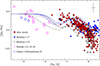 |
Fig. 4 [Zn/Fe] vs. [Fe/H] for the present sample (333 stars), compared with literature. Symbols: red filled circles: present work; black squares: results for stars in common based on UVES data (Barbuy et al. 2015); blue filled pentagons: Bensby et al. (2017); magenta open heptagons: Howes et al. (2015, 2016); blue open heptagons: Casey & Schlaufman (2015). Chemodynamical evolution models by FB17 with formation timescale of 2 (black lines) and 3 Gyr (blue lines), or specific star formation rate of 0.5, 0.3 Gyr−1 are overplotted. The model lines correspond to different radii from the Galactic centre: solid lines: r < 0.5 kpc; dotted lines: 0.5 < r < 1 kpc; dashed lines: 1 < r < 2 kpc; long-dashed lines: 2 < r < 3 kpc. A typical error bar is indicated in the right upper corner, corresponding to a mean between the two reference stars (Table 4). |
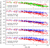 |
Fig. 5 [O, Mg, Si, Ca,Ti/Fe] vs. [Fe/H] and [Zn/Fe] vs. [Fe/H] for the 417 red giants. Symbols: Red filled circles: O from this work; Green filled circles: Zn from this work; Blue open triangles: Mg, Si, Ca, and Ti from Gonzalez et al. (2011). Typical error bars are indicated for [α/Fe] and [Zn/Fe]. |
4.2.1 Comparison with literature
Comparisons with literature Zn abundances of microlensed dwarf bulge stars by Bensby et al. (2013), were discussed in Barbuy et al. (2015). In Fig. 4 we show the updated abundances for microlensed bulge dwarfs by Bensby et al. (2017). There is good agreement between the present results and Barbuy et al. (2015) and those by Bensby et al. at metallicities −1.4 < [Fe/H] < 0.0, whereas the behaviour for metal-rich giants with [Fe/H] > 0.0 are distinct. The microlensed dwarfs show a contant [Zn/Fe], whereas the bulge red giants show a decreasing trend with metallicity, although with a large spread of −0.6 < [Zn/Fe] < +0.15.
At the high metallicity end, since there is progressive enrichment in Fe by SNIa, a constant [Zn/Fe] would imply that there is chemical enrichment in both Zn and Fe on similar timescales. Instead, a decrease of [Zn/Fe] would correspond to the enrichment in Fe by SNIa, with no enrichment in Zn by the same SNIa, as happens for the α-elements.
This discrepancy has been addressed by Duffau et al. (2017), who found, at supersolar metallicities, a decreasing [Zn/Fe] for red giants, and constant [Zn/Fe] for dwarfs. Their interpretation is that the dwarfs are old and the red giants are young. This interpretation cannot be applied here, given that at least part of the bulge metal-rich red giant stars should be old, as can be seen in the distribution of ages given in Bensby et al. (2017), see their Figs. 14 and 15).
The derivation of [Zn/Fe] in stars of dwarf galaxies by Skúladóttir et al. (2017; 2018, and references therein) indicated a decreasing [Zn/Fe] with increasing metallicities. This behaviour is in agreement with an Fe enrichment by SNIa, but not with a Zn enrichment.
4.2.2 Comparison with damped Lyman-alpha systems
Comparisons of Zn abundances with data from Akerman et al. (2005); Cooke et al. (2013), and Vladilo et al. (2011) were shown in Barbuy et al. (2015). Using careful dust corrections, Barbuy et al. (2015) concluded that the DLAs fall into the same region of [Zn/Fe] vs. [Fe/H] as thick disk and bulge stars. On the other hand, a comparison of the metallicity of DLAs to thick disk stars inRafelski et al. (2012) showed that while there is some overlap, the median DLA population is more metal poor than the thick disk stars. While Rafelski et al. (2012) did not apply dust corrections, metallicities were determined using primarily [Si/H] and [S/H], which are less sensitive to dust than [Zn/H]. To investigate this further, we compared the [Zn/Fe] vs. [Fe/H] from our present work to the DLA data presented in Rafelski et al. (2012) in Fig. 6. These data include a compilation of previous DLA systems selected to be unbiased with regard to their metallicities, including those from Akerman et al. (2005) and a subset of Vladilo et al. (2011). We note that the comparison in Fig. 6 must be taken with caution, because there are potential biases with the [Fe/Zn] values that are difficult to control. In the metal rich regime, Fe is strongly depleted by dust, while on the metal-poor side, the oscillator strengths of Zn result in theabsorption lines too weak to be detected in low-metallicity systems. To reduce the biases from dust depletion and undetected Zn absorption lines, we limited our comparison in Fig. 6 to systems with − 2.5 < [α∕H] < −1.0. In this comparison, no correction for dust is applied.
Figure 6a shows an enhanced zinc-to-iron ratio for the DLA data which is consistent with the present sample, although DLAs typically reside at lower metallicities. We note that Fig. 6 exaggerates the difference in metallicity ([Fe/H]) due to the removal of higher metallicity systems to avoid biases caused by dust depletion of Fe. Other literature data similarly show a spread in [Zn/Fe] (Akerman et al. 2005; Cooke et al. 2013 – see Barbuy et al. 2015), but is also compatible with a [Zn/Fe] enhancement. Cooke et al. (2015) argue instead that [Zn/Fe] in DLAs can be assumed to drop to solar at [Fe/H] ≈−2.0, based on a compilation of halo stars data by Saito et al. (2009). They assume therefore that Zn tracks Fe for [Fe/H] > −2.0. However, we show in Fig. 6a that both the present sample and the DLAs have elevated [Zn/Fe] at − 2.5 < [α∕H] < −1.0. Moreover, in Rafelski et al. (2012), we find that Zn and S trace each other one-to-one, not consistent with the solar value, but rather consistent with the models in Fenner et al. (2004), suggesting that Zn behaves like an α-element in DLAs, meaning that it is enhanced in metal-poor DLAs. In conclusion, Zn and α-elements show similar behaviour in metal-poor DLAs, and so can be expected to trace one another.
Figure 6a and b show a large scatter in the [Zn/Fe] and [α/Fe] in DLAs, due to varying star formation histories of the galaxies hosting DLAs, and due to variations of dust depletion for different sightlines. There may also be variations due to the complexities in the way Zn is produced. While Fe is produced in SNe Ia, Zn is produced in massive stars (WW95; Umeda & Nomoto 2002). The value of [Zn/Fe] in DLAs therefore likely depends on both the star formation histories of the host galaxies (Fenner et al. 2004) and on possible dust depletion in Fe for any individual sightline. Therefore a complementary investigation can be accomplished by studies of the α-enhancement [α/Fe] at [α/H] ≲−1.0.
Figure 6b shows an α-element enhancement of DLAs at [Fe/H] < −1.0 compared with [O/Fe] values for the present sample. In Fig. 6b we also include [O/Fe] values derived for metal-poor DLAs by Cooke et al. (2015). The enhanced [α/Fe] for stellar data with [Fe/H] < ~−0.6, is consistent with the alpha-element enhancement of the DLA data.
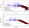 |
Fig. 6 Panela: [Zn/Fe] vs. [Fe/H]: same as in Fig. 4, including the damped Lyman-alpha systems data by Rafelski et al. (2012). Models from FB17 are overplotted (same details as in Fig. 4); panel b: [α/Fe] vs. [Fe/H]: data by Rafelski et al. (2012), [O/Fe] in DLAs by Cooke et al. (2015) and present results for [O/Fe] in the sample stars. The model lines in panel a: correspond to the same Galactic bulge radii as in Fig. 4. A typical error bar is indicated in the right upper corner in both panels: for [Zn/Fe] it corresponds to a mean value of the two reference stars given in Table 4. For [α/Fe] the error is of ±0.10 for both thestars and DLAs. |
5 Oxygen-poor, nitrogen-rich stars
Enhanced nitrogen is expected in red giants due to CN-cycle (Iben 1967), and extra-mixing (e.g. Smiljanic et al. 2009, as reviewed by Karakas & Lattanzio 2014, and references therein). The situation is different for N-rich and O-poor stars, which were first detected in globular clusters (e.g. Sneden et al. 1997). These stars are not only O-poor and N-rich, but also Na-rich, andanomalous also in Mg and Al. In the case of bulge red giants, Schiavon et al. (2017) identified N-rich stars, with a peak in metallicity at [Fe/H] ~−1.0. They included in this category stars with [N/Fe] ≳ +0.5, which in their sample of 5140 bulge giants, correspond to 58 of them, therefore in a proportion of 1.1%. Schiavon et al. interpreted these stars as second generation members evaporated from globular clusters. Carretta et al. (2009) have shown that second generation stars have low O, and high N and Na.
For this reason, for the N-rich as defined in Schiavon et al. (2017) with [N/Fe] ≳ +0.5 stars in our sample, we also measured their Na abundances, using the Na I 6154.23 and 6160.75 Å lines, adopting a hyperfine structure for total values of loggf = −1.56 and −1.26, respectively.The N-rich stars fall in different cases, in terms of N, O: (i) N-rich and O-poor, but for some of them we could not derive [O/Fe] due to blends with telluric lines, and only a N-enhancement is reported; (ii) N-rich and O-normal with [Fe/H] ≤−0.5; (iii) one star very N-rich [N/Fe] > 1.0 with [Fe/H] = +0.08 ([OI] line is blended with telluric lines in this case). These selected stars are listed in Table 6, where besides the [Na/Fe] value reported, [Mg/Fe] values are also given for an indication of the α-element enrichment in these stars as compared with the oxygen abundances.
If the criterion of [N/Fe] ≥ 0.5 for stars with [Fe/H] ≤−0.5, is adopted, we find 21 stars, corresponding to about 5% of the sample. If we consider the N-rich ones together with [Na/Fe] > 0.0, then we have 3.5% of them. Finally, if we discard the N-rich but O-normal, keeping only the O-poor ones ([O/Fe] ≲ 0.1), then we have five stars left, corresponding to about 1% of the sample, in agreement with the percentage given by Schiavon et al. (2017). It would be interesting to derive Al for these stars in order to verify a possible Mg-Al anticorrelation also detected in second generation globular cluster stars. The cause of these anomalies is currently under debate in the literature, with the more massive low-Z asymptotic giant branch stars as the likely site for such nucleosynthesis products (Renzini et al. 2015).
6 Summary
We studied oxygen and zinc abundances for 417 field red giants in the Galactic bulge. We were able to derive Zn, O, and N abundances for 333, 358 and 403 of them, respectively. We have identified five stars, corresponding to a 1% of stars that are simultaneously N-rich ([N/Fe] > 0.5), and O-poor ([O/Fe] ≲ 0.1), and this reduces to four stars if the more rigorous criterion of also being Na-rich ([Na/Fe] > 0.0) is applied. According to Schiavon et al. (2017), these characteristics could be attributed to evaporated second generation stars of globular clusters.
The sample contains a number of moderately metal-poor stars (−1.7 < [Fe/H] < −0.5) that define better the behaviour of [O/Fe] and [Zn/Fe] vs. [Fe/H] in this metallicity range. The present chemodynamical evolution modelling of a classical bulge is able to reproduce the behaviour of O and Zn abundances in the Galactic bulge, except for Zn in the range ~ −1.6 ≲ [Fe/H] ≲−0.8, where the yields from WW95 show a drop. We remind the reader that the models presented here consider yields from WW95 for [Fe/H] >−2.0, and a mean of models by WW95 and Kobayashi et al. (2006) for −4 < [Fe/H] < −2.
The high [Zn/Fe] in very metal-poor stars favours enrichment from hypernovae, as defined by Nomoto et al. (2013 and references therein) acting at these low metallicities. In damped Lyman-alpha systems (DLAs), a high [Zn/Fe] in metal-poor DLAs is also well reproduced by hypernovae yields. In DLAs Zn appears to behave similarly to α elements, and show an enhancement of [α/Fe] similar to the metal poor stars in the present sample. At the metal-rich end, a discrepancy persists between a decreasing [Zn/Fe] with increasing metallicity in the present sample of red giants, and an approximately constant [Zn/Fe] with metallicity for dwarf bulge stars. In conclusion, studies of the Galactic bulge with high-resolution spectroscopy for several hundred stars such as the present study, as well as work based on APOGEE data by Schiavon et al. (2017), and Schultheis et al. (2017), are crucial to better understand the chemical evolution and formation of the Galactic bulge.
Acknowledgements
CRS acknowledges a CAPES/PROEX PhD fellowship. BB and AF acknowledge partial financial support by CNPq, CAPES and FAPESP. MZ and DM acknowledge support by the Ministry of Economy, Development, and Tourism’s Millenium Science Initiative through grant IC120009, awarded to The Millenium Institute of Astrophysics, MAS, and from the BASAL Center for Astrophysics and Associated Technologies PFB-06 and FONDECYT Projects 1130196 and 1150345. SO acknowledges the Italian Ministero dell’Università e della Ricerca Scientifica e Tecnologica (MURST), Italy.
Appendix A Comparison between GIRAFFE and UVES spectra
Figures A.1 present the fits of the Zn I 6362.3 Å line, for both spectra GIRAFFE and UVES for stars in common between the two sets of observations.
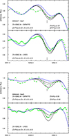 |
Fig. A.1 Comparison between UVES and Giraffe spectra with fits of the Zn I 6362.3 Å line, for stars in common. Symbols: dotted blackline and green filled triangles correspond to the observed spectra: black lines: synthetic spectra, dashed line: synthetic spectrum for the chosen [Zn/Fe] value. Blue solid line: synthetic spectra without Zn, showing the CN line. |
Appendix B Final abundances.
OGLE and GIRAFFE names, stellar parameters, resulting [N/Fe], [O/Fe], [Zn/Fe], and alpha-element abundances.
References
- Akerman, C. J., Ellison, S. L., Pettini, M., & Steidel, C. C. 2005, A&A, 440, 499 [NASA ADS] [CrossRef] [EDP Sciences] [Google Scholar]
- Alonso, A., Arribas, S., & Martínez-Roger, C. 1999, A&AS, 140, 261 [NASA ADS] [CrossRef] [EDP Sciences] [Google Scholar]
- Alves-Brito, A., Meléndez, J., Asplund, M., et al. 2010, A&A, 513, A35 [NASA ADS] [CrossRef] [EDP Sciences] [Google Scholar]
- Asplund, M., Grevesse, N., Sauval, A. J., & Scott, P. 2009, ARA&A, 47, 481 [NASA ADS] [CrossRef] [Google Scholar]
- Barbuy, B. 1988, A&A, 191, 121 [NASA ADS] [Google Scholar]
- Barbuy, B., Perrin, M.-N., Katz, D., et al. 2003, A&A, 404, 661 [NASA ADS] [CrossRef] [EDP Sciences] [Google Scholar]
- Barbuy, B., Hill, V., Zoccali, M., et al. 2013, A&A, 559, A5 [NASA ADS] [CrossRef] [EDP Sciences] [Google Scholar]
- Barbuy, B., Friaça, A., da Silveira, C. R., et al. 2015, A&A, 580, A40 [NASA ADS] [CrossRef] [EDP Sciences] [Google Scholar]
- Barbuy, B., Chiappini, C., & Gerhard, O. 2018, ARA&A, submitted, [arXiv:1805.01142] [Google Scholar]
- Bensby, T., Feltzing, S., & Lundström, I. 2004, A&A, 415, 155 [NASA ADS] [CrossRef] [EDP Sciences] [Google Scholar]
- Bensby, T., Yee, J. C., Feltzing, S., et al. 2013, A&A, 549, A147 [NASA ADS] [CrossRef] [EDP Sciences] [Google Scholar]
- Bensby, T., Feltzing, S., & Oey, M. S. 2014, A&A, 562, A71 [NASA ADS] [CrossRef] [EDP Sciences] [Google Scholar]
- Bensby, T., Feltzing, S., Gould, A., et al. 2017, A&A, 605, A89 [NASA ADS] [CrossRef] [EDP Sciences] [Google Scholar]
- Carpenter, J. M. 2001, AJ, 121, 2851 [NASA ADS] [CrossRef] [Google Scholar]
- Carretta, E., Bragaglia, A., Gratton, R. G., et al. 2009, A&A, 505, 117 [NASA ADS] [CrossRef] [EDP Sciences] [Google Scholar]
- Casey, A. R, & Schlaufman, K. C. 2015, ApJ, 809, 110 [NASA ADS] [CrossRef] [Google Scholar]
- Cavichia, O., Mollá, M., Costa, R. D. D., & Maciel, W. J. 2014, MNRAS, 437, 3688 [NASA ADS] [CrossRef] [Google Scholar]
- Cayrel, R., Depagne, E., Spite, M., et al. 2004, A&A, 416, 1117 [NASA ADS] [CrossRef] [EDP Sciences] [Google Scholar]
- Cescutti, G., Matteucci, F., Lanfranchi, G. A., & McWilliam, A. 2008, A&A, 491, 401 [NASA ADS] [CrossRef] [EDP Sciences] [Google Scholar]
- Coelho, P., Barbuy, B., Meléndez, J., Schiavon, R. P., & Castilho, B. V. 2005, A&A, 443, 735 [NASA ADS] [CrossRef] [EDP Sciences] [Google Scholar]
- Cooke, R., Pettini, M., Jorgenson, R. A., et al., 2013, MNRAS, 431, 1625 [NASA ADS] [CrossRef] [Google Scholar]
- Cooke, R. J., Pettini, M., & Jorgenson, R. A. 2015, ApJ, 800, 12 [NASA ADS] [CrossRef] [Google Scholar]
- Cunha, K., & Smith, V. V. 2006, ApJ, 651, 491 [NASA ADS] [CrossRef] [Google Scholar]
- Davis, S. P., & Phillips, J. G. 1963, The Red System (A2Π −X2Σ) of the CN molecule (Berkeley: University of California Press) [Google Scholar]
- Duffau, S., Caffau, E., Sbordone, L., et al. 2017, A&A, 605, A128 [NASA ADS] [CrossRef] [EDP Sciences] [Google Scholar]
- Fenner, Y., Prochaska, J. X., & Gibson, B. K 2004, ApJ, 606, 116 [NASA ADS] [CrossRef] [Google Scholar]
- Friaça, A. C. S., & Barbuy, B. 2017, A&A, 598, A121 [NASA ADS] [CrossRef] [EDP Sciences] [Google Scholar]
- Fulbright, J. P., McWilliam, A., & Rich, R. M. 2007, ApJ, 661, 1152 [NASA ADS] [CrossRef] [Google Scholar]
- Gaia Collaboration (Clementini, G., et al.) 2017, A&A, 605, A79 [NASA ADS] [CrossRef] [EDP Sciences] [Google Scholar]
- García-Pérez, A. E., Cunha, K., Shetrone, M., et al. 2013, ApJ, 767, L9 [NASA ADS] [CrossRef] [Google Scholar]
- Gonzalez, O. A., Rejkuba, M., Zoccali, M., et al. 2011, A&A, 530, A54 [NASA ADS] [CrossRef] [EDP Sciences] [Google Scholar]
- Gustafsson, B., Edvardsson, B., Eriksson, K., et al. 2008, A&A, 486, 951 [NASA ADS] [CrossRef] [EDP Sciences] [Google Scholar]
- Hawkins, K., Jofré, P., Masseron, T., & Gilmore, G. 2015, MNRAS, 453, 758 [NASA ADS] [CrossRef] [Google Scholar]
- Hill, V., Lecureur, A., Gómez, A., et al. 2011, A&A, 534, A80 [NASA ADS] [CrossRef] [EDP Sciences] [Google Scholar]
- Howes, L. M. 2015, PhD Thesis, Australian National University [Google Scholar]
- Howes, L. M., Asplund, M., Casey, A. R., et al. 2014, MNRAS, 445, 4241 [NASA ADS] [CrossRef] [Google Scholar]
- Howes, L. M., Casey, A. R., Asplund, M., et al. 2015, Nature, 527, 484 [NASA ADS] [CrossRef] [Google Scholar]
- Howes, L. M., Asplund, M., Keller, S. C., et al. 2016, MNRAS, 460, 884 [NASA ADS] [CrossRef] [Google Scholar]
- Iben, I. Jr. 1967, ARA&A, 5, 571 [NASA ADS] [CrossRef] [Google Scholar]
- Irwin, A. W. 1988, A&AS, 74, 145 [NASA ADS] [Google Scholar]
- Ishigaki, M. N., Aoki, W., & Chiba, M. 2013, ApJ, 771, 67 [NASA ADS] [CrossRef] [Google Scholar]
- Johnson, C. I., Rich, R. M., Kobayashi, C., Kunder, A., & Koch, A. 2014, AJ, 148, 67 [NASA ADS] [CrossRef] [Google Scholar]
- Jönsson, H., Ryde, N., Schultheis, M., & Zoccali, M. 2017, A&A, 600, A2 [Google Scholar]
- Karakas, A. I., & Lattanzio, J. C. 2014, PASA, 31, 30 [Google Scholar]
- Kobayashi, C., Umeda, H., Nomoto, K., Tominaga, N., & Ohkubo, T. 2006, ApJ, 643, 1145 [NASA ADS] [CrossRef] [Google Scholar]
- Lamb, M., Venn, K., Andersen, D. et al. 2017, MNRAS, 465, 3536 [NASA ADS] [CrossRef] [Google Scholar]
- Lecureur, A., Hill, V., Zoccali, M., Barbuy, B., et al. 2007, A&A, 465, 799 [NASA ADS] [CrossRef] [EDP Sciences] [Google Scholar]
- McWilliam, A. 2016, PASA, 33, 40 [NASA ADS] [CrossRef] [Google Scholar]
- Meléndez, J., Asplund, M., Alves-Brito, A., et al. 2008, A&A, 484, L21 [Google Scholar]
- Mikolaitis, S., Hill, V., Recio-Blanco, A., et al. 2014, A&A, 572, A33 [NASA ADS] [CrossRef] [EDP Sciences] [Google Scholar]
- Mishenina, T. V., Gorbaneva, T. I., Basak, N. Y., et al. 2011, Astron. Rep. 55, 689 [Google Scholar]
- Momany, Y., Vandame, B., Zaggia, S., et al. 2001, A&A, 379, 436 [NASA ADS] [CrossRef] [EDP Sciences] [Google Scholar]
- Ness, M., Freeman, K., Athanassoula, E., et al. 2013, MNRAS, 430, 836 [NASA ADS] [CrossRef] [Google Scholar]
- Nissen, P. E., & Schuster, W. J. 2011, A&A, 530, A15 [NASA ADS] [CrossRef] [EDP Sciences] [Google Scholar]
- Nomoto, K., Tominaga, N., Umeda, H., Kobayashi, C., & Maeda, K. 2006, Nucl. Phys. A, 777, 424 [NASA ADS] [CrossRef] [Google Scholar]
- Nomoto, K., Kobayashi, C., & Tominaga, N. 2013, ARA&A, 51, 457 [NASA ADS] [CrossRef] [Google Scholar]
- Pettini, M., Ellison, S. L., Steidel, C. C., & Bowen, D. V. 1999, ApJ, 510, 576 [NASA ADS] [CrossRef] [Google Scholar]
- Prochaska, J. S., Naumov, S. O., Carney, B. W., McWilliam, A., & Wolfe, A. M. 2000, AJ, 120, 2513 [NASA ADS] [CrossRef] [Google Scholar]
- Rafelski, M., Wolfe, A. M., Prochaska, J. X., et al. 2012, ApJ, 755, 89 [NASA ADS] [CrossRef] [Google Scholar]
- Rafelski, M., Neeleman, M., Fumagalli, M., et al. 2014, ApJ, 782, L29 [NASA ADS] [CrossRef] [Google Scholar]
- Ramírez, I., & Meléndez, J. 2005, ApJ, 626, 465 [NASA ADS] [CrossRef] [Google Scholar]
- Reddy, B. E., Lambert, D. L., & Allende Prieto, C. 2006, MNRAS, 367, 1329 [NASA ADS] [CrossRef] [Google Scholar]
- Renzini, A., D’Antona, F., Cassisi, S., et al. 2015, MNRAS, 454, 4197 [NASA ADS] [CrossRef] [Google Scholar]
- Rich, R. M., & Origlia, L. 2005, ApJ, 634, 1293 [NASA ADS] [CrossRef] [MathSciNet] [Google Scholar]
- Rich, R. M., Origlia, L., & Valenti, E. 2012, ApJ, 746, 59 [NASA ADS] [CrossRef] [Google Scholar]
- Rojas-Arriagada, A., Recio-Blanco, A., de Laverny, P., et al. 2017, A&A, 601, A140 [NASA ADS] [CrossRef] [EDP Sciences] [Google Scholar]
- Ryde, N., Gustafsson, B., Edvardsson, B., et al. 2010, A&A, 509, A20 [NASA ADS] [CrossRef] [EDP Sciences] [Google Scholar]
- Saito, Y.-J., Takada-Hidai, M., Honda, S., & Takeda, Y. 2009, PASJ, 61, 549 [NASA ADS] [Google Scholar]
- Schiavon, R. P., Zamora, O., Carrera, R., et al. 2017, MNRAS, 465, 501 [NASA ADS] [CrossRef] [Google Scholar]
- Schlafly, E. F., & Finkbeiner, D. P. 2011, ApJ, 737, 103 [NASA ADS] [CrossRef] [Google Scholar]
- Schultheis, M., Rojas-Arriagada, A., García-Pérez, A. E., et al. 2017, A&A, 600, A14 [NASA ADS] [CrossRef] [EDP Sciences] [Google Scholar]
- Siqueira-Mello, C., Chiappini, C., Barbuy, B., et al. 2016, A&A, 593, A79 [NASA ADS] [CrossRef] [EDP Sciences] [Google Scholar]
- Skúladóttir,Á., Tolstoy, E., Salvadori, S., Hill, V., & Pettini, M. 2017, A&A, 606, A71 [NASA ADS] [CrossRef] [EDP Sciences] [Google Scholar]
- Skúladóttir,Á., Salvadori, S., Pettini, M., Tolstoy, E., & Hill, V. 2018, A&A, in press, DOI: 10.1051/0004-6361/201732359 [Google Scholar]
- Smiljanic, R., Gauderon, R., North, P., et al. 2009, A&A, 502, 267 [NASA ADS] [CrossRef] [EDP Sciences] [Google Scholar]
- Sneden, C., Kraft, R. P., Shetrone, M. D., et al. 1997, AJ, 114, 1964 [NASA ADS] [CrossRef] [Google Scholar]
- Steffen, M., Prakapavicius, D., Caffau, E., et al. 2015, A&A, 583, A57 [NASA ADS] [CrossRef] [EDP Sciences] [Google Scholar]
- Tsuji, T. 1973, A&A, 23, 411 [NASA ADS] [Google Scholar]
- Udalski, A., Szymanski, M., Kubiak, M., et al. 2002, Acta Astron. 52, 217 [NASA ADS] [Google Scholar]
- Umeda, H., & Nomoto, K. 2002, ApJ, 565, 385 [NASA ADS] [CrossRef] [Google Scholar]
- Umeda, H., & Nomoto, K. 2003, Nature, 422, 871 [NASA ADS] [CrossRef] [PubMed] [Google Scholar]
- Umeda, H., & Nomoto, K. 2005, ApJ, 619, 427 [NASA ADS] [CrossRef] [Google Scholar]
- Vladilo, G., Abate, C., Yin, J., Cescutti, G., & Matteucci, F. 2011, A&A, 530, A33 [NASA ADS] [CrossRef] [EDP Sciences] [Google Scholar]
- Wise, J. H., Turk, M. J., Norman, M. L., & Abel, T. 2012, ApJ, 745, 50 [NASA ADS] [CrossRef] [Google Scholar]
- Woosley, S. E., & Weaver, T. A. 1995, ApJS, 101, 181 [NASA ADS] [CrossRef] [Google Scholar]
- Woosley, S., Heger, A., & Weaver, T. A. 2002, Rev. Mod. Phys., 74, 1015 [NASA ADS] [CrossRef] [Google Scholar]
- Zoccali, M., Lecureur, A., Barbuy, B., et al. 2006, A&A, 457, L1 [NASA ADS] [CrossRef] [EDP Sciences] [Google Scholar]
- Zoccali, M., Hill, V., Lecureur, A., et al. 2008, A&A, 486, 177 [NASA ADS] [CrossRef] [EDP Sciences] [Google Scholar]
- Zoccali, M., Vasquez, S., Gonzalez, O. A., et al. 2017, A&A, 599, A12 [NASA ADS] [CrossRef] [EDP Sciences] [Google Scholar]
ϵ(X) = log(n(X)∕n(H)) + 12, where n = number density of atoms, is a standard notation.
All Tables
Fields observed: coordinates, distance to Galactic centre, reddening as adopted in Zoccali et al. (2008), number of stars observed, and typical signal-to-noise ratios.
Sample of 23 stars observed with both FLAMES-UVES, and FLAMES-GIRAFFE for comparison purposes.
Uncertainties on the derived [O/Fe] and [Zn/Fe] values for model changes of Δ Teff = 150, 200 K, Δ log g = + 0.2, 0.4, Δ vt = +0.1, 0.2, 0.3 km s−1, for UVES and GIRAFFE data respectively, and corresponding total error, applied to the stellar parameters Teff, log g, [Fe/H], vt of stars BW-b6 (4200 K, 1.7, −0.25, 1.3 km s−1), and B6-b3 (4700 K, 2.0, 0.10, 1.6 km s−1).
Sample of stars observed with both FLAMES-UVES, and reanalysed by Jönsson et al. (2017).
OGLE and GIRAFFE names, stellar parameters, resulting [N/Fe], [O/Fe], [Zn/Fe], and alpha-element abundances.
All Figures
|
Fig. 1 Comparison between GIRAFFE and UVES abundances for O, N, and Zn for the stars common to the two sets of spectra (Table 3). For Zn: orange full circles consider the mean of two lines in the UVES results, and violet full triangles compare results for the same line. |
| In the text | |
|
Fig. 2 CNO abundances rederived for stars BW-f1 B6-b3, B6-f8, adopting stellar parameters defined by Jönsson et al. (2017). Symbols: black dotted line: observed spectra; blue solid line: synthetic spectra. |
| In the text | |
|
Fig. 3 [O/Fe] vs. [Fe/H] for 351 red giants (excluding N-rich, O-poor ones). Chemodynamical evolution models from FB17 with formation timescale of 2 Gyr, or specific star formation rate of 0.5 Gyr−1 are overplotted. Solid lines: 5 < 0.5 kpc; dotted lines: 0.5 < r < 1 kpc; dashed lines: 1 < r < 2 kpc; long-dashed lines: 2 < r < 3 kpc. Symbols: red filled circles: present work; green filled circles: Friaça & Barbuy (2017); blue stars: Jönsson et al. (2017); black stars: Ryde et al. (2010); grey filled squares: Schultheis et al. (2017); magenta open circles: García-Pérez et al. (2013); blue open circles: Howes et al. (2016); green open circles: Lamb et al. (2017). Errors indicated correspond to 0.1dex in both [Fe/H] and [O/Fe]. The model lines correspond to different radii from the Galactic centre: solid lines: r < 0.5 kpc; dotted lines: 0.5 < r < 1 kpc; dashed lines: 1 < r < 2 kpc; long-dashed lines: 2 < r < 3 kpc. A typical error bar is indicated in the right upper corner. |
| In the text | |
|
Fig. 4 [Zn/Fe] vs. [Fe/H] for the present sample (333 stars), compared with literature. Symbols: red filled circles: present work; black squares: results for stars in common based on UVES data (Barbuy et al. 2015); blue filled pentagons: Bensby et al. (2017); magenta open heptagons: Howes et al. (2015, 2016); blue open heptagons: Casey & Schlaufman (2015). Chemodynamical evolution models by FB17 with formation timescale of 2 (black lines) and 3 Gyr (blue lines), or specific star formation rate of 0.5, 0.3 Gyr−1 are overplotted. The model lines correspond to different radii from the Galactic centre: solid lines: r < 0.5 kpc; dotted lines: 0.5 < r < 1 kpc; dashed lines: 1 < r < 2 kpc; long-dashed lines: 2 < r < 3 kpc. A typical error bar is indicated in the right upper corner, corresponding to a mean between the two reference stars (Table 4). |
| In the text | |
|
Fig. 5 [O, Mg, Si, Ca,Ti/Fe] vs. [Fe/H] and [Zn/Fe] vs. [Fe/H] for the 417 red giants. Symbols: Red filled circles: O from this work; Green filled circles: Zn from this work; Blue open triangles: Mg, Si, Ca, and Ti from Gonzalez et al. (2011). Typical error bars are indicated for [α/Fe] and [Zn/Fe]. |
| In the text | |
|
Fig. 6 Panela: [Zn/Fe] vs. [Fe/H]: same as in Fig. 4, including the damped Lyman-alpha systems data by Rafelski et al. (2012). Models from FB17 are overplotted (same details as in Fig. 4); panel b: [α/Fe] vs. [Fe/H]: data by Rafelski et al. (2012), [O/Fe] in DLAs by Cooke et al. (2015) and present results for [O/Fe] in the sample stars. The model lines in panel a: correspond to the same Galactic bulge radii as in Fig. 4. A typical error bar is indicated in the right upper corner in both panels: for [Zn/Fe] it corresponds to a mean value of the two reference stars given in Table 4. For [α/Fe] the error is of ±0.10 for both thestars and DLAs. |
| In the text | |
|
Fig. A.1 Comparison between UVES and Giraffe spectra with fits of the Zn I 6362.3 Å line, for stars in common. Symbols: dotted blackline and green filled triangles correspond to the observed spectra: black lines: synthetic spectra, dashed line: synthetic spectrum for the chosen [Zn/Fe] value. Blue solid line: synthetic spectra without Zn, showing the CN line. |
| In the text | |
Current usage metrics show cumulative count of Article Views (full-text article views including HTML views, PDF and ePub downloads, according to the available data) and Abstracts Views on Vision4Press platform.
Data correspond to usage on the plateform after 2015. The current usage metrics is available 48-96 hours after online publication and is updated daily on week days.
Initial download of the metrics may take a while.