| Issue |
A&A
Volume 612, April 2018
|
|
|---|---|---|
| Article Number | A69 | |
| Number of page(s) | 14 | |
| Section | Numerical methods and codes | |
| DOI | https://doi.org/10.1051/0004-6361/201731438 | |
| Published online | 27 April 2018 | |
Exploring the inner parsecs of active galactic nuclei using near-infrared high resolution polarimetric simulations with MontAGN
1
LESIA, Observatoire de Paris, PSL Research University, CNRS, Sorbonne Universités, UPMC Univ. Paris 06, Univ. Paris Diderot, Sorbonne Paris Cité,
5 place Jules Janssen,
92190
Meudon, France
e-mail: This email address is being protected from spambots. You need JavaScript enabled to view it.
2
LUTH, Observatoire de Paris, CNRS, Université Paris Diderot, Sorbonne Paris Cité,
5 place Jules Janssen,
92190
Meudon, France
3
Univ. Grenoble Alpes, IRAM,
38000
Grenoble, France
4
LERMA, Observatoire de Paris, PSL Research University, CNRS, Sorbonne Universités, UPMC Univ. Paris 06, École normale supérieure,
75005
Paris, France
5
Observatoire Astronomique de Strasbourg, Université de Strasbourg, CNRS, UMR 7550,
11 rue de l’Université,
67000
Strasbourg, France
Received:
24
June
2017
Accepted:
22
November
2017
Abstract
Aims. In this paper we aim to constrain the properties of dust structures in the central first parsecs of active galactic nuclei (AGN). Our goal is to study the required optical depth and composition of different dusty and ionised structures.
Methods. We developed a radiative transfer code called Monte Carlo for Active Galactic Nuclei (MontAGN), which is optimised for polarimetric observations in the infrared. With both this code and STOKES, designed to be relevant from the hard X-ray band to near-infrared wavelengths, we investigate the polarisation emerging from a characteristic model of the AGN environment. For this purpose, we compare predictions of our models with previous infrared observations of NGC 1068, and try to reproduce several key polarisation patterns revealed by polarisation mapping.
Results. We constrain the required dust structures and their densities. More precisely, we find that the electron density inside the ionisation cone is about 2.0 × 10⁹ m−3. With structures constituted of spherical grains of constant density, we also highlight that the torus should be thicker than 20 in term of K-band optical depth to block direct light from the centre. It should also have a stratification in density: a less dense outer rim with an optical depth at 2.2 μm typically between 0.8 and 4 for observing the double scattering effect previously proposed.
Conclusions. We bring constraints on the dust structures in the inner parsecs of an AGN model supposed to describe NGC 1068. When compared to observations, this leads to an optical depth of at least 20 in the Ks band for the torus of NGC 1068, corresponding to τV ≈ 170, which is within the range of current estimation based on observations. In the future, we will improve our study by including non-uniform dust structures and aligned elongated grains to constrain other possible interpretations of the observations.
Key words: galaxies: Seyfert / techniques: polarimetric / techniques: high angular resolution / methods: numerical / radiative transfer
© ESO 2018
1 Introduction
Polarimetric observations are one of the key methodologies used to investigate the nature of active galactic nuclei (AGN), as was demonstrated 30 years ago in the study of Antonucci (1984) on optical polarisation of radio-loud AGN and of Antonucci & Miller (1985) who discovered broad Balmer lines and Fe II emission in the polarised light of NGC 1068, the archetypal Seyfert 2 galaxy.
Based on previous observations of the zoology of AGN (see e.g. Rowan-Robinson 1977; Neugebauer et al. 1980; Lawrence & Elvis 1982; Antonucci 1984), it was suspected that a circumnuclear obscuring region was responsible for the disappearance of the broad-line region in Seyfert 2, only revealed in AGN seen from directions around the pole (type 1 view). Following this idea, Antonucci (1993) proposed the unified model for radio-quiet AGN, stating that Seyfert 1 or 2 were the same type of object harbouring a luminous accretion disc surrounded by a thick torus, but seen at different viewing angles. This model has been thoroughly tested for many years by several observers, such as Gratadour et al. (2003), Das et al. (2006), or Lopez-Rodriguez et al. (2015), and compared to many simulations (see e.g. Wolf & Henning 1999; Marin 2014, 2016), who found a zeroth-order agreement with empirical measures. However, for the torus, one of the most important pieces of the model, we still lack information due to its limited extension and to the high contrast required to observe it. Constraints were recently brought thanks to adaptive optics (AO), polarisation, and interferometry. Raban et al. (2009) detected two components in the centre of NGC 1068 using mid-infrared interferometry, while Gratadour et al. (2015) used high angular resolution polarimetry to detect the likely signature of the core of the same AGN in near-infrared (NIR). More recently, García-Burillo et al. (2016) used ALMA to map the submillimetre counterpart of the torus, finding a molecular disc of about 10 pc diameter.
With the addition of polarimetry, we have access to information that is less affected by the intensity contrast between the torus signal and the extremely bright central core than it would be with spectroscopy, interferometry, or imaging alone. In addition to intensity, we can measure information about the oscillation directions of the electromagnetic field, translated into three additional and independent parameters: the linear polarisation degree, the polarisation position angle, and the circular polarisation (rarely measured).
Polarisation gives clues on the history of the successive interactions of light with matter. Photons can be emitted already polarised if the source is, for instance, composed of elongated and aligned grains (see e.g. Efstathiou et al. 1997), but light can also become polarised if scattered or if there is unbalanced absorption by aligned grains. Polarisation is therefore a powerful tool for studying the properties of scatterers such as dust grains or electrons in AGN environments. Polarimetric measurements can also help to disentangle the origin of polarisation between spherical and oblate grains, as discussed in Lopez-Rodriguez et al. (2015), and to put constraints on the properties of the magnetic fields around the source as it is likely to align non-spherical dust grains. This would be seen as polarised light through dichroic emission and absorption (see Packham et al. 2007). The downside of this method is that interpretation of polarimetric data, with multiple possible origins, is not straightforward and requires a proper modelling.
Following the NIR observations of NGC 1068 by Gratadour et al. (2015), we developed a numerical simulation code to interpret the observed polarisation features, namely a central region with a low degree of polarisation at a constant position angle with a ridge of higher polarisation degree at the very centre. In this paper, the general context and reference observations are presented inSect. 2 and the numerical code is described in Sect. 3. We then present two sets of parameters: a toy AGN model, used to validate the output of the simulation code and a more realistic set of parameters used to reproduce our previous observations of NGC 1068 (Sect. 4). We analyse and discuss the simulation results in Sect. 5 before concluding.
2 Observational constraints
According to the unified model (Antonucci 1993), the structure of an AGN is assumed to be constituted of the three essential components represented in Fig. 1:
-
the central engine (CE), most likely to be a super massive black hole with a hot accretion disc emitting through unpolarised thermal emission most of the luminosity from ultraviolet to NIR;
-
the optically thick dusty torus, surrounding the CE and blocking the light in the equatorial plane, with its innermost border at sublimation temperature being a strong emitter in the near/mid-infrared;
-
an ionisation cone in the polar directions directly illuminated by the CE, diluted into the interstellar medium to create the narrow line region after a few tens of parsecs.
NGC 1068 is a typical Seyfert 2 galaxy, which has long been the main target for studies of AGN. It is indeed one of the most luminous and closest active nucleus (about 14.4 Mpc, following recommendation of Bland-Hawthorn et al. 1997) and therefore one of the brightest. For this reason we can reach higher resolution and better contrast between the CE and its close environment than we canwith other active galaxies. For this target, the nucleus can be used as the guide source for the AO system. Such high angular NIR observations have already been published, first obtained with NACO (Rouan et al. 2004; Gratadour et al. 2006) and more recently using SPHERE with polarimetric information (Gratadour et al. 2015).
The later observations were conducted during the SPHERE Science Verification (SV) programme in December 2014. H and Ks broad-band images were obtained, showing a polarisation angle map with a clear centrosymmetric pattern, tracing the ionisation cone. Additionally, a compact area of constant polarisation direction was observed at the centre of this hourglass shape and interpreted as a signature of the torus (see Fig. 2, extracted from Gratadour et al. 2015). Our assumption was that the optically thick torus would block direct light from the hottest dust and that we would be seeing light scattered twice. The first scattering would take place in the ionisation cone, allowing some photons to be redirected toward the outer part of the equatorial plane and then undergo a second scattering (see Fig. 3 for illustration). If we detect such photons, the signature would be a polarisation pattern aligned with the equatorial plane. This is an analogous phenomenon to the one observed in the envelope of young stellar objects (YSO) proposed by Bastien & Menard (1990) and Murakawa (2010). In this configuration, spherical grains can alone produce these signatures in polarisation images. This should constrain the optical depth of the different components, as we investigate here.
The torus is more likely to be clumpy as the hydrodynamic stability of tens of parsec scale structures is not well explained. Furthermore, fragmentation is usually invoked to explain some of the observations according to recent studies (Mason et al. 2009; Müller Sánchez et al. 2009; Nikutta et al. 2009; Alonso-Herrero et al. 2011). However, we will first examine models with uniform structures, each with a constant density to ease simulations and analysis. We have tested a range of optical depths between τV = 20 and 100 for the torus median plane. We based this choice on the current estimations of about 50 in the visible, as derived by e.g. Gratadour et al. (2003). We note that more recently, Lira et al. (2013) and Audibert et al. (2017) have found greater optical depths and that both these authors derived them assuming clumpy structures.
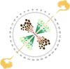 |
Fig. 1 Unscaled sketch of the AGN unification theory. A type 1 AGN is seen at inclinations 0°–60°, while a type 2 AGN is seen at approximately 60°–90°. Colour-coding: the central super massive black hole is in black, the surrounding X-ray corona is in violet, the multi-temperature accretion disc is shown with the colour pattern of a rainbow, the broad-line region is in red and light brown, the circumnuclear dust is in dark brown, the polar ionized winds are in dark green, and the final extension of the narrow line region is in light green. A double-sided, kilo-parsec jet is added to account for radio-loud AGN. From Marin et al. (2016a). |
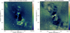 |
Fig. 2 NGC 1068 observed with SPHERE. Left panel: degree of linear polarisation; right panel: result of the difference between the polarisation angle map and a purely centrosymmetric pattern. Images from Gratadour et al. (2015). |
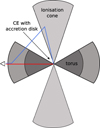 |
Fig. 3 Example of two photon paths on an AGN environment. The blue path has an integrated optical depth of about 1–4, while the red one is about 50–200. |
3 MontAGN simulation code
Because polarimetry is a complex phenomenon, radiative transfer codes are essential tools for the interpretation of these observations. However as far as we know, no radiative transfer code was able to address all wavelength ranges. Because of our particular requirements, we decided to develop our own simulation code optimised for AGN observations in the infrared. The Monte Carlo for Active Galactic Nuclei (MontAGN) code was designed to study whether our assumptions on single and double scattering with a proper torus geometry were valid and if this would allow us to reproduce the observed polarisation images of NGC 1068. The MontAGN code will be available to the public in the near future.
3.1 Overview
MontAGN is written in Python 2.7. It uses photon packets with constant initial energy instead of propagating single photons. This allows us to choose between two propagation techniques:
-
If re-emission is disabled, the energy of the packets is modified to take into account, at each event, the photon fraction of the initial packets that continues to propagate in the medium. Therefore, at each encounter with a grain, the absorbed fraction of photons is deduced so that only the scattered photons propagate. Murakawa (2010) used the same techniques for the simulations of YSO.
-
If re-emission is enabled, the code takes into account the absorption and re-emission by dust as well as temperature equilibrium adjustment at each absorption. If absorbed, the photon packet is re-emitted at another wavelength with the same energy but with a different number of photons. This keeps the energy constant within the cell. The re-emission wavelength is randomly selected in function of the temperature difference ΔT in the cell, after the packet’s absorption, following the method of Bjorkman & Wood (2001). By doing so, we take into account the previous re-emissions that were not emitted according to the final emission function. We therefore use the difference of spectrum between the two emissivity for both cell temperatures to emit the photon packets (see Fig. 4, taken from the previously cited paper) and correct the probability distribution function from the previous re-emissions.
The user can define whether the re-emission is enabled or not. By disabling it, every packet will propagate until it exits the medium and the number of packets collected at a given wavelength will be larger.1 Disabling this effect provides more statistics at the end of the simulation as every packet is taken into account; however, it also requires a minimum number of packets in each pixel of the final images as we can obtain in a given pixel only packets with very few photons because of successive scatterings with a low albedo, a situation that may not be representative of the actual pixel polarisation. This point is discussed in more detail in Sect. 5.1
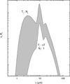 |
Fig. 4 Temperature correction frequency distribution. Shown are the dust emissivities, jν = κν Bν(T), prior to andafter the absorption of a single photon packet. The spectrum of the previously emitted packets is given by the emissivity at the old cell temperature (bottom curve). To correct the spectrum from the old temperature to the new temperature(upper curve), the photon packet should be re-emitted using the difference spectrum (shaded area). Image from Bjorkman & Wood (2001). |
3.2 Initialisation
The MontAGN code uses a 3D grid of cells, sampling the densities of the different dust species in each cell. Dust grains are considered as dielectric spheres. Before the simulation starts, tables of albedo, phase function, Mueller matrix, absorption, and extinction coefficients are generated for a range of grain sizes and wavelengths thanks to Mie theory. For that purpose, we use the bh_mie module initially written by Bohren & Huffman (1983). These tables then just need to be interpolated (linear or logarithmic interpolations) to get the precise value for a given set of grain sizes and wavelengths during the simulation. These interpolations make the execution of the code faster. MontAGN uses the Stokes vectors formalism to represent polarisation of photons packets,
 (1)
(1)
with I the intensity, Q and U the two components of linear polarisation, and V the circular polarisation. In MontAGN, we normalise the Stokes vector (I = 1) to simplify the Stokes vector propagation.
3.3 Photon propagation
When a packet is emitted, the source is selected according to the respective luminosity of each sources. The packet’s wavelength is determined using the source’s spectral energy distribution; the photons are initially not polarised (i.e. with Stokes vector of the photons set to [1,0,0,0]). The packet begins to propagate in a randomly chosen direction. At its first encounter with a non-empty cell, a value of the optical depth that the photon will be allowed to travel is randomly determined, as in Robitaille (2011). On its path, the photon’s “remaining optical depth” is reduced as a function of the densities of the dust species in the corresponding cells. When it reaches 0, the packet interacts with a grain of the cell: the radius of the grain is randomly chosen using the dust grain size function, and from this radius and the wavelength, albedo, phase function, scattering angles, and Mueller matrix are determined. In order to make the information on polarisation evolve, we apply the Mueller matrix and the rotation matrix to the Stokes vector:
 (2)
(2)
Here, M is the Mueller matrix constructed from Mie theory and R is the rotation matrix, both of which depend on the scattering angles. More information on matrices and the Stokes formalism can be found in Appendix A. A new optical depth is randomly determined after each scattering.
When the photon packet exits the simulation box, it is recorded with its four Stokes parameters, the number of interaction, its last interaction position, and its final direction of propagation registered in the form of two angles, inclination θ (ranging from 0° to 180°), and azimuth ϕ (ranging from 0° to 360°). From these data, Q and U maps are created, summing photons packets (with a possible selection on altitude and azimuthal angles) and combined in maps of polarisation angle and degree using
 (3)
(3)
 (4)
(4)
 (5)
(5)
If the model is axisymmetric, MontAGN allows the signal obtained from simulations to be increased following two assumptions. First, in the case of cylindrical symmetries, all the photons exiting the simulation with the same inclination angle θ but different azimuthal angle ϕ are equivalent. We can therefore use all photons with a θ in the proper range by performing a rotation around the vertical axis of the photon’s final position.
If the model is also symmetric according to the equatorial plane, photons recorded above the equatorial plane are equivalent to those below the plane. In the end we can add photons of the four quadrants (upper left, upper right, bottom left, and bottom right) as long as we properly change their polarisation properties according to the symmetry; however, it is mandatory to observe at an inclination angle of 90° when using this last method.
It is important to note that it is possible to define an upper bound for the number of absorptions that a photon packet undergoes in order to keep only packets transporting significant energy and have faster simulations. As this information is kept, it is also possible to get access to maps of the averaged number of interactions undergone in a particular direction.
3.4 Maps
As we record packets with different numbers of photons, we need to take these differences into account when creating the observed maps. All maps (including those referred to as “averaged”) are generated by summing photons instead of packets. The parameters2 of all packets are summed with a factor proportional to the fraction of remaining photons in each packet i (in each resolution element). As the number of photons is proportional to the energy, the energy Ei of the packets is used to weight the packets. The averaged number of scatterings n in a pixel of the map will therefore be computed from the number of scatterings of each packet ni as
 (6)
(6)
Packets are selected to compute the maps in a certain range of inclinations. In the following, we use the range ± 5° and the images computed at 90° therefore include photons exiting with an inclination in the range [85°,95°].
4 Models
4.1 First tests and toy models
We first conducted validation tests of the MontAGN code on YSO, using the geometry described in Murakawa (2010). Our results were compatible with those shown in their paper in terms of polarisation degree and angles, albeit with a higher Poissonian noise due to the very high optical depth involved in this model (about 6 × 10⁴ in K band). The clear polarisation angle pattern seen in Murakawa (2010, see their Fig. 6) needs more photons to be achieved. For a proper validation of AGNs, we defined a set of three models to compare the results of simulations between MontAGN and STOKES codes (Goosmann & Gaskell 2007; Marin et al. 2012, 2015) in a simple case. Detailed information on the comparison of the two codes can be found in Grosset et al. (2016). A first analysis and conclusions are also available in Marin et al. (2016b). As the two codes are not aimed to work in the same spectral bands, namely the infrared for MontAGN and the NIR, visible, UV, and X-rays for STOKES, we selected intermediate and overlapping wavelengths: 800, 900, and 1000 nm. Our baseline models were filled with silicates grains alone in the dustystructures and electrons in the ionisation cone. All grain data, including graphites used in other models, come from Draine (1985). All dust distributions were set to dielectric spheres with a radius ranging from 0.005 μm to 0.250 μm with a power law of −3.5, following the distribution defined in Mathis et al. (1977).
The three models are based on simple geometrical features with constant silicate or electron densities:
-
a flared dusty torus, ranging from 0.05 pc to 10 pc, a value consistent with what is currently estimated (Antonucci 1993; Kishimoto 1999; García-Burillo et al. 2016). It has a half opening angle of 30° from theequatorial plane and an optical depth of 50 at 500 nm in the equatorial plane;
-
an ionised outflow, composed of electrons in a bi-cone of half opening angle of 25° from thesymmetry axis of the model, from 0.05 pc to 25 pc at an optical depth of 0.1;
-
an outer dusty shell ranging from 10 pc to 25 pc, outside of the ionisation cone, with a radial optical depth of 0.5 at 500 nm.
The first model is built with these three components (model 1), the second with only the torus and the outflow (model 2), and the third is reduced to the torus only (model 3). See Fig. 5 for density maps of each model.
For eachof these models we launched 107 packets, disabling re-emission and considering only the above-mentioned wavelengths. All inclination angles were recorded. We show in Figs. 6 and 7 the maps obtained at 800 nm at an observing angle of 90° (edge-on).
As shown in Fig. 6, results between the two codes are in fairly good agreement, as expected from Grosset et al. (2016) and Marin et al. (2016b). The few observed differences likely arise from the divergence in the simulation strategy. Because MontAGN (in the configuration used here) propagates photons packets that may have suffered strong absorption, the pixels with a low number of photons may not contain reliable information in some cases (see Sect. 5.1). However, as the packets number increases, the maps converge toward a more realistic result, close to those produced with STOKES. In the central regions, we only have a few photons recorded. This is expected because escaping photons here have been scattered several times and their number decrease strongly at each interaction because of the low albedo. For this reason, the central regions differ slightly between STOKES and MontAGN results, especially in their outer parts.
In model 1, we get two different regions. First a central region mainly constituted of photons that have been scattered twice. The second region is separated into two polar areas of single scattering. These appear in blue in the maps in Fig. 7. As expected in this configuration (discussed in e.g. Fischer et al. 1996 and Whitney & Hartmann 1993), we observe in the north and south two well-defined regions of centrosymmetric polarisation position angle. In these two zones, photons are scattered with an angle close to 90°, which ensures a high degree of polarisation and a polarisation position angle orthogonal to the scattering plane, leading to this characteristic pattern.
The central belt is mostly dominated by the photons scattered twice. Therefore, it traces the regions that photons cannot exit easily without interaction because of the optical depth of the medium: these are the areas obscured by the torus. However, there is no clear privileged direction of polarisation angle in this central band. This is likely due to the surrounding medium which allows the first scattering to take place in any direction around the torus, a conclusion that leads us to the definition of model 5 (described in next section).
Model 2 only differs by the lack of the dust shell surrounding the torus. The signal clearly shows the ionisation cone as a region of single scattering, and the torus region. In this second area, the central signal does not trace photons scattered twice, but photons that undergo multiple scatterings (five or more). The role of the shell is therefore critical for the central signal we observe with model 1. It provides an optically thin region where photons can be scattered, without travelling through the optically thick torus (see Fig. 3).
This is confirmed by model 3, which reproduces quite well the results of model 2 in the torus field of view even though there is no ionisation cone where the photons can undergo their first scattering.
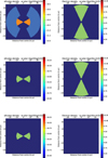 |
Fig. 5 Vertical slices of grain density of silicates (in log10(kg/m3), first column) and density of electrons (in log10(m−3), second column) set for model 1 (first row), model 2 (second row), and model 3 (third row). |
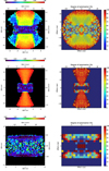 |
Fig. 6 Maps of polarisation degree with an inclination angle of 90° at 800 nm for models 1, 2, and 3. The first column shows maps from STOKES; the second column corresponds to MontAGN maps (in %). The first row is for model 1, the second row for model 2, and the third row for model 3 results. Polarisation vectors are shown: their lengths are proportional to the polarisation degree and their position angles represent the polarisation angle. |
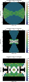 |
Fig. 7 Maps of observed averaged number of scatterings with an inclination angle of 90° at 800 nm for models 1, 2, and 3 with MontAGN. Polarisation vectors are shown: their lengths are proportional to the polarisation degree and their position angles represent the polarisation angle (p = 1 is represented by a length of a pixel size). |
4.2 Double scattering models
The simple models were not able to adequately reproduce the observed horizontal polarisation in the central inner parsecs of Gratadour et al. (2015), and so we added some features. Specifically, we increased the density of the torus to an optical depth of nearly 150 at 800 nm (model 4) and in a another model we replaced the outer shell by an extension of the torus with lower density (model 5; see Fig. 8 for the density maps).
For these models we used two different dust compositions: only silicates, and a mixture of graphites (parallel and orthogonal) and silicatesgrains. The ionisation cone contains only electrons in both cases. In the case of silicates and graphites, we used the following number ratios: 37.5% silicates, 41.7% orthogonal graphites (electric field oscillates perpendicular to the graphite plane), and 20.8% parallel graphites (electric field oscillates parallel to the graphite plane), based on Goosmann & Gaskell (2007). Other ratios could be considered, for example by using the work of Jones et al. (2013). Silicate and mixture models share the same τR.
We ran each of these models with 107 photon packets launched, without re-emission and considering only the wavelengths 800 nm and 1.6 μm. All inclination angles were recorded. In Figs. 9 and 10 we show maps derived from the MontAGN simulations. They correspond to maps of averaged number of scatterings with polarisation vectors (p = 1 is represented by a length of a pixel size), for models with the two dust compositions.
One should first notice that the dust composition slightly affects the results, mostly on the maps in Fig. 10. This is likely due to the difference in optical depth introduced by the difference in composition,3 as will be discussed in Sect. 5.3.
The centrosymmetric regions of model 4 are similar for both dust composition at 800 nm and 1.6 μm and are similar to the results of model 1. As the optical depth of the torus should not affect this part of the map, this is consistent. However, the results found with model 4 are very close to those observed with model 1, even in the central belt. In this region, mostof the photons undergo two scatterings at 800 nm for model 4, the only difference arises from the model with silicates where we see that a slightly larger fraction of photons have undergone more than two scattering events. At 1.6 μm, there are almost no photons coming from the regions shadowed by the torus on the outer central belt with the pure silicates model. Again this is an effect of optical depth (see Sect. 5.3)
Model 5 differs (second and fourth images of Figs. 9 and 10) more from the previous models. By adding a spatially limited region where photons can be scattered a second time, hidden by the torus from the emission of the source, we see a large region of double scattered light. Polarisation in this area in map at 800 nm shows a clear constant horizontal polarisation. This is not visible on the 1.6 μm map where the optical depth of the torus is not high enough to block photons coming directly from the AGN centre.
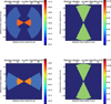 |
Fig. 8 Grain density of silicates (in log10 (kg m−3), first column) and electron density (in log10 (m−3), second column) set for model 4 (first row) and model 5 (second row) (shown here for the silicates-electron composition). |
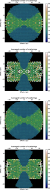 |
Fig. 9 Maps of observed averaged number of scattering with an inclination angle of 90° at 800 nm with MontAGN. Polarisation vectors are shown, their lengths being proportional to the polarisation degree and their position angles representing the polarisation angle. The first two images are for models with silicates and electrons, the last two images for models with silicates, graphites, and electrons. The first and third images correspond to model 4, the second and fourth to model 5. |
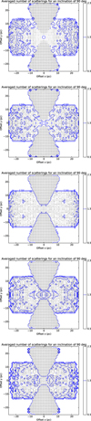 |
Fig. 11 Maps of the observed averaged number of scattering with an inclination angle of 90° at 1.6 μm with MontAGN. The optical depth of the cone is fixed to 0.1, that of the extended torus to 0.8, and that of the torus is respectively 5, 10, 20, 50, and 100 (in H band). |
4.3 Optical depth
In order to measure the impact and the importance of the optical depth, we ran a series of models based on model 5, differing only by the optical depth of their components. Among the three main parameters (the ionisation cone, the torus, and its extended region), we kept the density of two of them fixed and changed the last one. First we took models by varying the optical depth of the torus. Then, we changed the optical depth of the cone, and finally we studied a variation of the optical depth of the extended torus. The results are shown in Figs. 11, 12, and 13, respectively. Polarisation vectors are shown whose lengths are proportional to the polarisation degree and whose position angles represent the polarisation angle. All these models contains the same mixtures of silicates and graphites as in model 4, and 5. 2 × 10⁷ packets were launched per model, all at 1.6 μm where the optical depth is set. Some additional maps are available in Appendix B.
With the first series of simulations (Fig. 11), we obtain results that are similar to those of the previous cases. For a low optical depth of the torus, photons can travel without interaction through the torus and produce a centrosymmetric pattern, even in the central region. By increasing the density, the importance of these photons decreases until the double scattered light becomes predominant (around τ ≈ 20). At this step, increasing the optical depth does not seem to change the observed features significantly.
With the second and third series, the density of the two other structures must be in a certain range to obtain the constant horizontal polarisation pattern we are looking for. If these structures have an optical depth that is too low or too high, the central belt shows multiple scatterings as seen in both Figs. 12 and 13. In extreme cases with very high optical depth in the outer torus, we have no photons in this region, a case close to the simulations of model 2 (see Fig. 7). These two conditions seem to be important to produce the features we are expecting.
A last remark is that the photons detected from the ionisation cone are no longer just scattered once at high optical depth in the cone (Fig. 12). However, the centrosymmetric pattern seems to be approximatively conserved for double scattering in the cone.
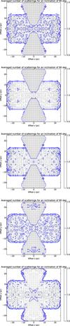 |
Fig. 12 Same as Fig. 11. The optical depth of the cone is respectively 0.05, 0.1, 0.5, 1.0, and 10.0, those of the torus and its extended part are fixed to 20 and 0.8 (in H band). |
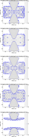 |
Fig. 13 Same as Figs. 11 and 12. The optical depth of the cone is 0.1, that of the extended torus respectively 0.4, 0.8, 4.0, 8.0, and 80.0. That of the torus is fixed to 20 (in H band). |
4.4 Reproducing the NGC 1068 observations
Based on previous simulations, we tried to reproduce the SPHERE observations of NGC 1068. As we observed constant polarisation orientation in the core of NGC 1068 in both the H and Ks bands, we need in our simulation an optical depth τ ≥ 20 at 2.2 μm to be able to generate such polarisation features. We changed our previous model 5 to adapt it to these larger wavelengths. Here, the torus has an optical depth τKs = 19, which gives τH = 35 and τV =169. We note that this is in therange of the current estimation of the density of dust in the torus (see Sect. 5.6). For this simulation we used a mixture of silicates and graphites to rely on a realistic dust composition for an AGN, inspired by Wolf & Henning (1999). We adapted their mass ratio to a number ratio according to Guillet (2008) leading to 57% silicates, 28.67% parallel graphites, and 14.33% orthogonal graphites.
With these parameters, the maps in Fig. 14 are now able to reproduce some of the observed features. Namely, the nearly constant horizontal polarisation in the central part is similar to that observed on NGC 1068 at 1.6 and 2.2 μm. We are, however, not yet able to reproduce the ridge that appears at the very centre of the SPHERE observations.
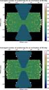 |
Fig. 14 Maps of the observed averaged number of scattering with an inclination angle of 90° at 1.6 (top) and 2.2 μm (bottom). Polarisation vectors are shown, their lengths being proportional to the polarisation degree and their position angles representing the polarisation angle. |
5 Discussion
5.1 Photons significance
One major concern is the simulation strategy of conserving the packets until they exit the simulation box, whatever their number of interactions.We must verify to what extent the detected photons are relevant. The energy of each packet is decreased according to the albedo at each interaction, as is the number of photons in the packet. Therefore, it is common at the end to record photon packets with energies 104 times lower than the initial energy. If a high energy packet reaches a pixel previously populated only with low energy ones, it will totally dominate the pixel so that Q and U values and the polarisation parameters will be essentially linked to this packet. Indeed, most of the photons in the pixel will be from this packet.
Unlike simulations including absorption, where all the recorded photons have the same probability, this is no longer the case here. A pixel of an output image could have stacked many low energy packets before a high energy one, more representative of the actual polarisation, can reach it. But it is also possible that no high power photon reaches this cell in the course of the simulation, leading to an incorrect estimate.
To analyse our results, we need first to be sure to distinguish between photons representative of the actual polarisation and those which are not. Limiting the number of scatterings is a good way to ensure that under a given limit of the number of photons, packets will stop being recorded. We also analysed maps of “effective number” of photon packets per pixel, as shown in Appendix B. These maps are generated by dividing the energy received in each pixel by the highest energy of packets recorded in the pixel. If a single packet dominates the pixel’s information, the effective number of packets in the pixel will be close to 1, indicating a non-reliable pixel.
As the energy of packets decreases with the number of scatterings, regions where there are a low number of scatterings are more likely to be reliable. All regions of single-scattered photons, with the exception of the central pixels, are reliable as long as photons cannot reach the pixel in this region directly without being scattered. For the same reasons, all the regions with photons scattered twice on average are very likely to be representative, because only single-scattered packets have higher energies.
5.2 Effect of geometry
In the ionisation cone, we are able to reproduce the observed centrosymmetric pattern at a large distance from the centre. This is expected from photons that are scattered only once (see e.g. Marin et al. 2012). The maps of the average number of scatterings confirms that in all these regions we see mainly photons that are only scattered once.
More interesting is the central region. We are able to reproduce with model 5 (Fig. 9) a horizontal polarisation, at least at 800 nm. This is comparable to what was obtained in the case of YSO by Murakawa (2010, see e.g. their Fig. 6). The case of YSOs, however, is very different from AGN in terms of optical depth, which is about 6.0 × 10⁵ in the K band in the equatorial plane. However, the geometry of the dust distribution has some similarities, with two jets in the polar directions and a thick dusty environment surrounding the central source. We based our interpretation of the pattern observed in NGC 1068 on the effect called the “roundabout effect” by Bastien & Menard (1990) and used by Murakawa (2010) to describe the path of photons in YSOs. In AGN environments, despite an optically thick torus, we do not expect such high optical depth. Studies tend to argue for optical depth lower than 300 in the visible, as discussed in Sect. 5.6.
As said before, to be able to see horizontal polarisation with only spherical grains, it is necessary to have a region beyond the torus with a lower optical depth at the considered wavelength (typically under 10) for the photons to be scattered a second time toward the observer. This is realistic because one can expect the external part of the torus to be diluted into the interstellar medium with a smooth transition. The theory of disc wind being at the origin of torus, described in e.g. Elitzur & Ho (2009), would support such a dilution.
The ionisation cone is an important piece as it is required for the first scattering. However, while comparing the results of models 1 and 5, it seems important to have a collimated region for this first scattering to happen; all photons will have almost the same scattering plane, which therefore leads to a narrow range of polarisation position angle. This is not the case in model 1 where photons could interact not only in the ionisation cone, but also in the whole outer shell.
We note that all the tested geometries are rather simple in terms of structures and their edges are sharp. One of the advantages of using a 3D grid for sampling dust density is the capability to reproduce more complex structures with filaments or clumps. These are, however, more complex in terms of polarisation signatures (see Marin et al. 2015; Marin & Schartmann 2017) and we therefore limited ourselves to simple models in this first paper. For further studies, we aim to develop more realistic models. In particular, MontAGN will be able to incorporate density structures from AGN hydrodynamical simulations (Rybicki et al. 1990; Pereyra et al. 1997; Proga et al. 2000; Hopkins et al. 2012), which could help, for example, to constrain the wind geometry and launching mechanism (see Marin & Goosmann 2013).
5.3 Dust composition
Dust composition also has an effect on the polarisation maps. As the graphites and silicates do not have the same absorption coefficient dependence on wavelength for a given optical depth in the V band, the optical depth will be different in the H or K band. For instance with τV ≈ 50, we have τH ≈ 2.7 in the silicates case and τH ≈ 11.6 with the mixture of graphites and silicates (because of the difference in extinction coefficient, as seen in Fig. 15).
This also explains why there are almost no photons in the equatorial belt of the upper panel of Fig. 10 (only silicates), as opposed to the case with silicates and graphites. The extended torus region indeed has in the pure silicate model a low optical depth at 1.6 μm and photonshave a low probability of interacting in this area, making the signal in the equatorial belt hard to detect. This will be discussed and used later to study the role of the optical depth in the outer torus.
We also observed that in the cone, the flux due to scattering on electrons is stronger than that coming from scattering on silicate grains. This difference stems directly from the absorption properties. Silicates through Rayleigh scattering and electrons with Thomson scattering have the same scattering phase functions. However, electrons have an absorption coefficient of 0, while the silicates’coefficient is close to 1 and depends on the wavelength.
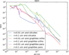 |
Fig. 15 Extinction coefficient Qext in function of wavelength, grain radius, and grain type (data from Draine 1985). |
5.4 Thick torus
In order for the photons scattered twice to be dominant in the central region, it is necessary to have an optical depth high enough in the equatorial plane. If not, photons coming directly from the source, with a single scattering or no scattering will contaminate the observed polarisation and even become dominant (see Sect. 5.1). The switch from one regime to the other is when the probability for a photon to emerge from the dust having suffered at most one scattering is of the same order as the probability of a photon being scattered twice. We note that because electrons do not absorb photons, they are much more efficient than dust grains for the same optical depth. Even with electrons in the cone, photons have to be redirected in the correct solid angle toward the equatorial plane and to be scattered again without being absorbed in the observer’s direction. The favourable cases to observe this signal seems to be for optical depths higher than 20 in the equatorial plane, as determined from Fig. 11.
This conclusion is in agreement with the observation that no broad-line emission is detected in total flux when the AGN is viewed edge-on. With a lower optical depth torus, we would have been able to detect such broad lines directly through the torus. This is not the case, as demonstrated by e.g. Antonucci & Miller (1985) on NGC 1068 and Ramos Almeida et al. (2016) on a larger sample, who revealed these hidden lines only thanks to polarimetry.
5.5 Optical depth of scattering regions
Another important parameter is the density of the matter in the cone and in the extended part of the torus. If both areas are at low density, photons have a lower probability of following the roundabout path and are less likely to produce the horizontal pattern, as seen in Fig. 12. But if the optical depth is too high in the cone and/or in the outskirts of the torus, typically of the order of 1–2, photons have a low probability of escaping from the central region and will never be observed. We can see in the last two panels of Fig. 12 that the averaged number of scatterings in the cone is greater than 1, and that the signal of the photons scattered twice becomes weaker in the central belt. The range of values which favour the constant polarisation signal in the centre is around 0.1–1.0 in the cone and 0.8–4.0 in the extended region of the torus. For the outer torus this corresponds to a density about 20 times lower than in the torus.
We can therefore underline the importance of these two parameters and especially the extension of the torus. When comparing these results to the previous models, we noticed that in the first panel of Figs. 9 and 10, we observe few photons in the centre of the 800 nm image and almost none on the 1.6 μm one. The optical depth of the torus is lower in the second case and this region is therefore more easily reached by photons in this configuration. The only factor that can explain this lack of photon at 1.6 μm is the optical depth difference in the outer shell, which is of the order of 0.5 at 800 nm and much lower in the NIR, compared to the 0.8 lower limit determined previously. The structure, composition, and density of the torus (including its outer part) therefore all intervene to determine the polarisation pattern in the median plane. To be observable, the horizontal polarisation requires a proper combination of the parameters within a rather narrow range.
5.6 Consequences for observations
In Fig. 14 one can see that there are very few differences between H band and Ks band images. The optical depth of 169 in V band required for these images is acceptable, being in the range of present estimations. Marin et al. (2015) use values of optical depth in the range 150–750 in the visible, while Gratadour et al. (2003) derived τV =40. Assuming clumpy structures, Alonso-Herrero et al. (2011) obtained optical depths of about 50 in V per cloud fitting mid-IR spectral energy distributions of NGC 1068. Lira et al. (2013) and Audibert et al. (2017) more recently found integrated values of optical depth of about 250, based on fits of the NIR and mid-IR spectral energy distributions of samples of Seyfert 1 and 2 galaxies. We have to keep in mind that all these optical depths are derived assuming clumpy structure, so we should be careful when comparing them to optical depths of continuous dust distributions because the masses of the dust are very different. It is in our plans to explore the effect of a clumpy structure, a capability already implemented in MontAGN.
A part of the polarisation may arise from elongated aligned grains as studied by Efstathiou et al. (1997). If so, the required optical depth could change. This might explain the observed ridge on the polarimetric images of NGC 1068 and aligned elongated grains are therefore something we should investigate further. However, the exact mechanism of this alignment in this configuration on a rather large scale (60 pc) is still to be established. For instance, if due to magnetic field, it would require a toroidal component because we expect the polarisation pattern to be parallel with the magnetic field in the case of dichroic absorption as discussed in Lopez-Rodriguez et al. (2015).
Our interpretation does not require special properties of grains (elongated and/or aligned) and indeed, spherical dust grains in the torus coupled to electrons in the ionisation cone are able to reproduce the polarisation orientation in the central belt. In this case we constrain the optical depth of the structures to a rather narrow range of values. In the cone,the range of optical depth is between 0.1 and 1.0. A value of 0.1 gives an electron density of 2.0 ×10⁹ m−3, which is consistent with the estimated range in AGN (108 –1011 m−3 for NGC 1068 according to Axon et al. 1998; Lutz et al. 2000).
The only feature that our simulations do not seem to reproduce is the ridge at the very centre of NGC 1068 (Gratadour et al. 2015). Investigating a model with non-spherical grains could potentially solve this problem through dichroism.
6 Conclusion and prospectives
In this paper, we described and used the radiative transfer code with polarimetric capabilities MontAGN to study the inner dust structures of AGN, especially NGC 1068, in which the observed polarisation pattern is compatible with the idea of photons that are scattered twice proposed by Bastien & Menard (1990) and later validated by Murakawa (2010) on YSOs. This was the basis of our analysis of our observations of NGC 1068 (Gratadour et al. 2015). The code allows us to simulate NIR polarimetric observations of an AGN featuring an ionisation cone, a torus, and an extended envelope.
Despite limiting ourselves to a simple case where the various structures have a constant density of dust or electrons, we are able with spherical grains only, to constrain the optical depth of the different dust structures, thus obtaining a similar polarisation pattern to the one observed on NGC 1068.
We highlight the important role of both the ionisation cone and the dusty torus. The cone allows photons to be scattered toward the equatorial plane. In order for this redirection to be efficient, we found that electrons are much more satisfactory than dust grains because they are non-absorbing, a hint that these cones are more likely populated by electrons, as suspected by Antonucci & Miller (1985). We estimate the optical depth in the ionisation cone, measured vertically, to be in the range 0.1–1.0 in the first 25 parsecs from the AGN.
We found that for the light directly coming from the central region of the AGN to be blocked, the torus should have an in-plane integrated optical depth greater than 20 in the considered band, so τKs ≥ 20 in the case of NGC 1068. Furthermore, the torus should not only be constituted of an optically thick dense part, but also of an almost optically thin extended part. We find satisfactory results with an outer part with optical depth 0.8 < τH < 4.0 and an extension ranging from 10 pc to 25 pc from the centre. We considered structures with constant density as something unrealistic, but we expect similar results for a more continuous torus with a density decreasing with distance to the centre. This is a direction in which we aim to carry our study in the near future.
There are other improvements we will be able to conduct. One major amelioration will be to include elongated aligned grains. As already mentioned, another improvement is the introduction of a clumpy torus instead of constant density structures. We also aim to include the “peeling-off” technique (Yusef-Zadeh et al. 1984) in MontAGN in order to obtain a larger photon sample for a given inclination when simulating the polarisation signal of a peculiar object. A net gain of computation time is expected, at the expense of all other inclinations.
Acknowledgements
The authors would like to acknowledge financial support from the Programme National Hautes Energies (PNHE) and from “Programme National de Cosmologie and Galaxies” (PNCG) funded by CNRS/INSU-IN2P3-INP, CEA, and CNES, France.
Appendix A: Stokes formalism and Mueller matrices
In order to compute the evolution of polarisation through scattering, MontAGN uses the Stokes formalism. It requires two matrices to compute the new Stokes vector after the scattering event. The Mie theory gives the values of S1 and S2, which are determined for each wavelength, grain type, grain radius, and scattering angle. These two quantities are linked to the electrical properties of the material and are used to compute the elements of the Mueller matrix:
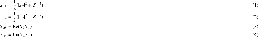
The Mueller matrix is defined as
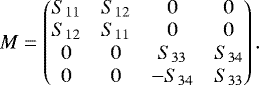 (A.5)
(A.5)
By applying the Mueller matrix to the Stokes vector, we take into account the change in the polarisation introduced by the main scattering angle (α) between the incoming ray and the new direction of propagation.
 (A.6)
(A.6)
which gives
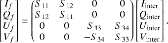 (A.7)
(A.7)
However, as the scattering is not necessary in the previous polarisation plane of the photon, we need to translate the old photon’s polarisation into the new frame used for the scattering. For this purpose we use a rotation matrix defined as
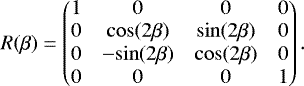 (A.8)
(A.8)
The rotation matrix is mandatory to modify the polarisation plane according to the scattering geometry and depends on β, the azimuthal scattering angle. We then switch to Sfinal from Sinitial by applying both matrices:
 (A.9)
(A.9)
and in detailed form:
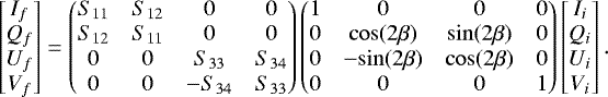 (A.10)
Appendix B: Additional maps
Here are shown some of the additional maps computed from model 5 in Sect. 4.3 at 1.6 μm in which the optical depth of the cone is fixed to 0.1, those of the extended torus to 0.8, and that of the torus to 20 (in H band) (Figs. B.1 and B.2).
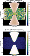 |
Fig. B.1 Maps of the observed linear polarisation degree (top) and of the effective number of packets (bottom, the effective number of packets is defined in Sect. 5.1) with an inclination angle of 90° at 1.6 μm. |
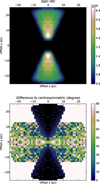 |
Fig. B.2 Maps of observed Q tangential (top, corresponds to the image of the centrosymmetric polarised intensity), and of difference angle to centrosymmetric pattern (bottom), as computed in Gratadour et al. (2015), with an inclination angle of 90° at 1.6 μm. |
Appendix C: MontAGN pseudo-code
General MontAGN algorithm:
-
MontAGN 01 Reading of the input parameters and conversion into corresponding class objects. Parallelisation if asked.
-
MontAGN 02 Reading of the parameters for dust geometry (given as keyword, asked or from parameter file): dust densities, grains properties, and structures associated.
-
MontAGN 03 Creation of the 3D grid and filling in of dust densities: computation of the density of each grain type for each cell. Temperature initialisation.
-
MontAGN 04 Computation of the tables of all propagation elements: Mueller matrices, albedo, Qabs, Qext, phase functions, for each grain type and different wavelength/grain radius.
-
MontAGN 05 Start of the simulation.
-
MontAGN 06 Selection of a source based on relative luminosity.
-
MontAGN 07 Determination of the photon wavelengths and initial directions of propagation and of polarisation. The wavelength is randomly determined from the source’s spectral energy distribution. The Stokes vector and propagation vectors are initialised.
-
MontAGN 08 Propagation of the packet until a non-empty cell is reached:
-
Determination of the cell density;
-
If null, direct determination of the next cell, back to the beginning of MontAGN 08;
-
If radius smaller than sublimation radius, the cell is considered empty.
-
MontAGN 09 Determination of a τ that the packet will be able to penetrate, computed by inversion from optical depth penetration definition P(τx > τ) = e−τ.
-
MontAGN 10 Determination of the next event of the packet:
-
Interaction if τ is too low to allow the packet to exit the cell;
-
Or exit from the cell (in that case, decrease of τ and going to MontAGN 18).
-
MontAGN 11 Determination of the properties of the encountered grain/electron: size and therefore albedo, Qabs and Qext.
-
MontAGN 12
Case 1 (no re-emission): decrease in the energy of the packet according to the albedo (and going to MontAGN 16).
Case 2 (re-emission): determination whether the packet is absorbed from albedo.
If no, go to MontAGN 16.
-
MontAGN 13 Determination of the new temperature of the cell from the previous one by equalising incoming and emitted energy.
-
MontAGN 14 If the new temperature is above the sublimation temperature of a type of grain, update of the sublimation radius of this type of grains.
-
MontAGN 15 Determination of the new wavelength and direction of propagation of the packet. The directions are determined randomly, the wavelength is determined from the difference between new and old temperatures of the cell.
Go to MontAGN 18.
-
MontAGN 16 Determination of the angles of scattering and of the new directions of propagation and polarisation:
-
From grain properties and wavelength, determination of the scattering angle α and of the Muller Matrix components S1 and S2;
-
Determination of scattering angle β;
-
Computation of the new propagation vectors.
-
MontAGN 17 Construction of the matrices. From the angles, S1 and S2, construction of Mueller matrix and of the rotation matrix (as described in Appendix A). Application to Stokes vector of the packet.
-
MontAGN 18 If the packet is still in the simulation box, go back to MontAGN 10, else the packet exits the simulation.
-
MontAGN 19 Computation of the packet properties in the observer’s frame. From the propagation vectors, determination of the orientation of the polarisation frame and correction of Stokes parameters using a rotation matrix.
-
MontAGN 20 Recording of the packet’s properties by writing it in the files specified.
-
MontAGN 21 If there are still other packets to launch, go back to MontAGN 06.
-
MontAGN 22 End of simulation.
-
MontAGN 23 Computation of the displays if asked.
References
- Alonso-Herrero, A., Ramos Almeida, C., Mason, R., et al. 2011, ApJ, 736, 82 [NASA ADS] [CrossRef] [Google Scholar]
- Antonucci, R. R. J. 1984, ApJ, 278, 499 [NASA ADS] [CrossRef] [Google Scholar]
- Antonucci, R. 1993, ARA&A, 31, 473 [Google Scholar]
- Antonucci, R. R. J., & Miller, J. S. 1985, ApJ, 297, 621 [NASA ADS] [CrossRef] [Google Scholar]
- Audibert, A., Riffel, R., Sales, D. A., Pastoriza, M. G., & Ruschel-Dutra, D. 2017, MNRAS, 464, 2139 [NASA ADS] [CrossRef] [Google Scholar]
- Axon, D. J., Marconi, A., Capetti, A., et al. 1998, ApJ, 496, L75 [NASA ADS] [CrossRef] [Google Scholar]
- Bastien, P., & Menard, F. 1990, ApJ, 364, 232 [NASA ADS] [CrossRef] [Google Scholar]
- Bjorkman, J. E., & Wood, K. 2001, ApJ, 554, 615 [NASA ADS] [CrossRef] [Google Scholar]
- Bland-Hawthorn, J., Gallimore, J. F., Tacconi, L. J., et al. 1997, Ap&SS, 248, 9 [NASA ADS] [CrossRef] [Google Scholar]
- Bohren, C. F., & Huffman, D. R. 1983, Absorption and Scattering of Light by Small Particles (New York: John Wiley & Sons) [Google Scholar]
- Das, V., Crenshaw, D. M., Kraemer, S. B., & Deo, R. P. 2006, AJ, 132, 620 [NASA ADS] [CrossRef] [Google Scholar]
- Draine, B. T. 1985, ApJS, 57, 587 [NASA ADS] [CrossRef] [Google Scholar]
- Efstathiou, A., McCall, A., & Hough, J. H. 1997, MNRAS, 285, 102 [NASA ADS] [CrossRef] [Google Scholar]
- Elitzur, M. & Ho, L. C. 2009, ApJ, 701, L91 [NASA ADS] [CrossRef] [Google Scholar]
- Fischer, O., Henning, T., & Yorke, H. W. 1996, A&A, 308, 863 [NASA ADS] [Google Scholar]
- García-Burillo, S., Combes, F., Ramos Almeida, C., et al. 2016, ApJ, 823, L12 [NASA ADS] [CrossRef] [Google Scholar]
- Goosmann, R. W., & Gaskell, C. M. 2007, A&A, 465, 129 [NASA ADS] [CrossRef] [EDP Sciences] [Google Scholar]
- Gratadour, D., Clénet, Y., Rouan, D., Lai, O., & Forveille, T. 2003, A&A, 411, 335 [NASA ADS] [CrossRef] [EDP Sciences] [Google Scholar]
- Gratadour, D., Rouan, D., & Mugnier, L. M., et al. 2006, A&A, 446, 813 [NASA ADS] [CrossRef] [EDP Sciences] [Google Scholar]
- Gratadour, D., Rouan, D., Grosset, L., Boccaletti, A., & Clénet, Y. 2015, A&A, 581, L8 [NASA ADS] [CrossRef] [EDP Sciences] [Google Scholar]
- Grosset, L., Marin, F., Gratadour, D., et al. 2016, in SF2A-2016: Proc. Annual Meet. French Soc. Astron. Astrophys., eds. C. Reylé, J. Richard, L. Cambrésy, et al., 57 [Google Scholar]
- Guillet, V. 2008, Theses, Université Paris Sud, Paris XI, France [Google Scholar]
- Hopkins, P. F., Hayward, C. C., Narayanan, D., & Hernquist, L. 2012, MNRAS, 420, 320 [NASA ADS] [CrossRef] [Google Scholar]
- Jones, A. P., Fanciullo, L., Köhler, M., et al. 2013, A&A, 558, A62 [NASA ADS] [CrossRef] [EDP Sciences] [Google Scholar]
- Kishimoto, M. 1999, ApJ, 518, 676 [NASA ADS] [CrossRef] [Google Scholar]
- Lawrence, A., & Elvis, M. 1982, ApJ, 256, 410 [NASA ADS] [CrossRef] [Google Scholar]
- Lira, P., Videla, L., Wu, Y., et al. 2013, ApJ, 764, 159 [NASA ADS] [CrossRef] [Google Scholar]
- Lopez-Rodriguez, E., Packham, C., Jones, T. J., et al. 2015, MNRAS, 452, 1902 [NASA ADS] [CrossRef] [Google Scholar]
- Lutz, D., Sturm, E., Genzel, R., et al. 2000, ApJ, 536, 697 [NASA ADS] [CrossRef] [Google Scholar]
- Marin, F. 2014, MNRAS, 441, 551 [NASA ADS] [CrossRef] [Google Scholar]
- Marin, F. 2016, MNRAS, 460, 3679 [NASA ADS] [CrossRef] [Google Scholar]
- Marin, F., & Goosmann, R. W. 2013, MNRAS, 436, 2522 [NASA ADS] [CrossRef] [Google Scholar]
- Marin, F., & Schartmann, M. 2017, A&A, 607, A37 [NASA ADS] [CrossRef] [EDP Sciences] [Google Scholar]
- Marin, F., Goosmann, R. W., Gaskell, C. M., Porquet, D., & Dovčiak, M. 2012, A&A, 548, A121 [NASA ADS] [CrossRef] [EDP Sciences] [Google Scholar]
- Marin, F., Goosmann, R. W., & Gaskell, C. M. 2015, A&A, 577, A66 [Google Scholar]
- Marin, F., Goosmann, R. W., & Petrucci, P.-O. 2016a, A&A, 591, A23 [NASA ADS] [CrossRef] [EDP Sciences] [Google Scholar]
- Marin, F., Grosset, L., Goosmann, R., et al. 2016b, in SF2A-2016: Proc. Annual Meet. French Soc. Astron. Astrophys., eds. C. Reylé, J. Richard, L. Cambrésy, et al., 103 [Google Scholar]
- Mason, R. E., Levenson, N. A., Shi, Y., et al. 2009, ApJ, 693, L136 [NASA ADS] [CrossRef] [Google Scholar]
- Mathis, J. S., Rumpl, W., & Nordsieck, K. H. 1977, ApJ, 217, 425 [NASA ADS] [CrossRef] [Google Scholar]
- Müller Sánchez, F., Davies, R. I., Genzel, R., et al. 2009, ApJ, 691, 749 [NASA ADS] [CrossRef] [Google Scholar]
- Murakawa, K. 2010, A&A, 518, A63 [NASA ADS] [CrossRef] [EDP Sciences] [Google Scholar]
- Neugebauer, G., Morton, D., Oke, J. B., et al. 1980, ApJ, 238, 502 [NASA ADS] [CrossRef] [Google Scholar]
- Nikutta, R., Elitzur, M., & Lacy, M. 2009, ApJ, 707, 1550 [NASA ADS] [CrossRef] [Google Scholar]
- Packham, C., Young, S., Fisher, S., et al. 2007, ApJ, 661, L29 [NASA ADS] [CrossRef] [Google Scholar]
- Pereyra, N. A., Kallman, T. R., & Blondin, J. M. 1997, ApJ, 477, 368 [NASA ADS] [CrossRef] [Google Scholar]
- Proga, D., Stone, J. M., & Kallman, T. R. 2000, ApJ, 543, 686 [NASA ADS] [CrossRef] [Google Scholar]
- Raban, D., Jaffe, W., Röttgering, H., Meisenheimer, K., & Tristram, K. R. W. 2009, MNRAS, 394, 1325 [NASA ADS] [CrossRef] [Google Scholar]
- Ramos Almeida, C., Martínez González, M. J., Asensio Ramos, A., et al. 2016, MNRAS, 461, 1387 [NASA ADS] [CrossRef] [Google Scholar]
- Robitaille, T. P. 2011, A&A, 536, A79 [NASA ADS] [CrossRef] [EDP Sciences] [Google Scholar]
- Rouan, D., Lacombe, F., Gendron, E., et al. 2004, A&A, 417, L1 [NASA ADS] [CrossRef] [EDP Sciences] [Google Scholar]
- Rowan-Robinson, M. 1977, ApJ, 213, 635 [NASA ADS] [CrossRef] [Google Scholar]
- Rybicki, G. B., Owocki, S. P., & Castor, J. I. 1990, ApJ, 349, 274 [NASA ADS] [CrossRef] [Google Scholar]
- Whitney, B. A., & Hartmann, L. 1993, ApJ, 402, 605 [NASA ADS] [CrossRef] [Google Scholar]
- Wolf, S., & Henning, T. 1999, A&A, 341, 675 [NASA ADS] [Google Scholar]
- Yusef-Zadeh, F., Morris, M., & White, R. L. 1984, ApJ, 278, 186 [NASA ADS] [CrossRef] [Google Scholar]
This is only true if the signal in the wavelength range mainly originates from the centre (hottest dust or CE); it is the opposite when looking at wavelengths where emission come mostly from direct dust re-emission (typically in the mid-infrared).
Mainly the intensities I, Q, U, and V, but also the number of scatterings, for example.
The optical depth is the same as in R, but it evolves differently depending on the dust composition.
All Figures
|
Fig. 1 Unscaled sketch of the AGN unification theory. A type 1 AGN is seen at inclinations 0°–60°, while a type 2 AGN is seen at approximately 60°–90°. Colour-coding: the central super massive black hole is in black, the surrounding X-ray corona is in violet, the multi-temperature accretion disc is shown with the colour pattern of a rainbow, the broad-line region is in red and light brown, the circumnuclear dust is in dark brown, the polar ionized winds are in dark green, and the final extension of the narrow line region is in light green. A double-sided, kilo-parsec jet is added to account for radio-loud AGN. From Marin et al. (2016a). |
| In the text | |
|
Fig. 2 NGC 1068 observed with SPHERE. Left panel: degree of linear polarisation; right panel: result of the difference between the polarisation angle map and a purely centrosymmetric pattern. Images from Gratadour et al. (2015). |
| In the text | |
|
Fig. 3 Example of two photon paths on an AGN environment. The blue path has an integrated optical depth of about 1–4, while the red one is about 50–200. |
| In the text | |
|
Fig. 4 Temperature correction frequency distribution. Shown are the dust emissivities, jν = κν Bν(T), prior to andafter the absorption of a single photon packet. The spectrum of the previously emitted packets is given by the emissivity at the old cell temperature (bottom curve). To correct the spectrum from the old temperature to the new temperature(upper curve), the photon packet should be re-emitted using the difference spectrum (shaded area). Image from Bjorkman & Wood (2001). |
| In the text | |
|
Fig. 5 Vertical slices of grain density of silicates (in log10(kg/m3), first column) and density of electrons (in log10(m−3), second column) set for model 1 (first row), model 2 (second row), and model 3 (third row). |
| In the text | |
|
Fig. 6 Maps of polarisation degree with an inclination angle of 90° at 800 nm for models 1, 2, and 3. The first column shows maps from STOKES; the second column corresponds to MontAGN maps (in %). The first row is for model 1, the second row for model 2, and the third row for model 3 results. Polarisation vectors are shown: their lengths are proportional to the polarisation degree and their position angles represent the polarisation angle. |
| In the text | |
|
Fig. 7 Maps of observed averaged number of scatterings with an inclination angle of 90° at 800 nm for models 1, 2, and 3 with MontAGN. Polarisation vectors are shown: their lengths are proportional to the polarisation degree and their position angles represent the polarisation angle (p = 1 is represented by a length of a pixel size). |
| In the text | |
|
Fig. 8 Grain density of silicates (in log10 (kg m−3), first column) and electron density (in log10 (m−3), second column) set for model 4 (first row) and model 5 (second row) (shown here for the silicates-electron composition). |
| In the text | |
|
Fig. 9 Maps of observed averaged number of scattering with an inclination angle of 90° at 800 nm with MontAGN. Polarisation vectors are shown, their lengths being proportional to the polarisation degree and their position angles representing the polarisation angle. The first two images are for models with silicates and electrons, the last two images for models with silicates, graphites, and electrons. The first and third images correspond to model 4, the second and fourth to model 5. |
| In the text | |
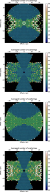 |
Fig. 10 Same as Fig. 9, but at 1600 nm. |
| In the text | |
|
Fig. 11 Maps of the observed averaged number of scattering with an inclination angle of 90° at 1.6 μm with MontAGN. The optical depth of the cone is fixed to 0.1, that of the extended torus to 0.8, and that of the torus is respectively 5, 10, 20, 50, and 100 (in H band). |
| In the text | |
|
Fig. 12 Same as Fig. 11. The optical depth of the cone is respectively 0.05, 0.1, 0.5, 1.0, and 10.0, those of the torus and its extended part are fixed to 20 and 0.8 (in H band). |
| In the text | |
|
Fig. 13 Same as Figs. 11 and 12. The optical depth of the cone is 0.1, that of the extended torus respectively 0.4, 0.8, 4.0, 8.0, and 80.0. That of the torus is fixed to 20 (in H band). |
| In the text | |
|
Fig. 14 Maps of the observed averaged number of scattering with an inclination angle of 90° at 1.6 (top) and 2.2 μm (bottom). Polarisation vectors are shown, their lengths being proportional to the polarisation degree and their position angles representing the polarisation angle. |
| In the text | |
|
Fig. 15 Extinction coefficient Qext in function of wavelength, grain radius, and grain type (data from Draine 1985). |
| In the text | |
|
Fig. B.1 Maps of the observed linear polarisation degree (top) and of the effective number of packets (bottom, the effective number of packets is defined in Sect. 5.1) with an inclination angle of 90° at 1.6 μm. |
| In the text | |
|
Fig. B.2 Maps of observed Q tangential (top, corresponds to the image of the centrosymmetric polarised intensity), and of difference angle to centrosymmetric pattern (bottom), as computed in Gratadour et al. (2015), with an inclination angle of 90° at 1.6 μm. |
| In the text | |
Current usage metrics show cumulative count of Article Views (full-text article views including HTML views, PDF and ePub downloads, according to the available data) and Abstracts Views on Vision4Press platform.
Data correspond to usage on the plateform after 2015. The current usage metrics is available 48-96 hours after online publication and is updated daily on week days.
Initial download of the metrics may take a while.