| Issue |
A&A
Volume 611, March 2018
|
|
|---|---|---|
| Article Number | L4 | |
| Number of page(s) | 13 | |
| Section | Letters to the Editor | |
| DOI | https://doi.org/10.1051/0004-6361/201732528 | |
| Published online | 28 March 2018 | |
Letter to the Editor
The magnetic nature of umbra–penumbra boundary in sunspots
1
Astronomical Institute of the Academy of Sciences,
Fričova 298,
25165
Ondřejov, Czech Republic
e-mail: This email address is being protected from spambots. You need JavaScript enabled to view it.
2
Instituto de Astrofísica de Canarias (IAC), Vía Lactéa,
38200
La Laguna,
Tenerife, Spain
3
Departamento de Astrofísica, Universidad de La Laguna,
38205
La Laguna,
Tenerife, Spain
4
Kiepenheuer-Institut für Sonnenphysik,
Schöneckstr. 6,
79104
Freiburg, Germany
5
The Czech Academy of Sciences, Institute of Information Theory and Automation,
Pod vodárenskou věží 4,
182 08
Praha, Czech Republic
Received:
22
December
2017
Accepted:
22
January
2018
Abstract
Context. Sunspots are the longest-known manifestation of solar activity, and their magnetic nature has been known for more than a century. Despite this, the boundary between umbrae and penumbrae, the two fundamental sunspot regions, has hitherto been solely defined by an intensity threshold.
Aim. Here, we aim at studying the magnetic nature of umbra–penumbra boundaries in sunspots of different sizes, morphologies, evolutionary stages, and phases of the solar cycle.
Methods. We used a sample of 88 scans of the Hinode/SOT spectropolarimeter to infer the magnetic field properties in at the umbral boundaries. We defined these umbra–penumbra boundaries by an intensity threshold and performed a statistical analysis of the magnetic field properties on these boundaries.
Results. We statistically prove that the umbra–penumbra boundary in stable sunspots is characterised by an invariant value of the vertical magnetic field component: the vertical component of the magnetic field strength does not depend on the umbra size, its morphology, and phase of the solar cycle. With the statistical Bayesian inference, we find that the strength of the vertical magnetic field component is, with a likelihood of 99%, in the range of 1849–1885 G with the most probable value of 1867 G. In contrast, the magnetic field strength and inclination averaged along individual boundaries are found to be dependent on the umbral size: the larger the umbra, the stronger and more horizontal the magnetic field at its boundary.
Conclusions. The umbra and penumbra of sunspots are separated by a boundary that has hitherto been defined by an intensity threshold. We now unveil the empirical law of the magnetic nature of the umbra–penumbra boundary in stable sunspots: it is an invariant vertical component of the magnetic field.
Key words: Sun: magnetic fields / Sun: photosphere / sunspots
© ESO 2018
1 Introduction
The enhanced temperature and brightness of a penumbra compared to temperature and brightness of an umbra define a sharp intensity boundary between these regions. This umbral boundary is commonly outlined by an intensity threshold of 50% relative to the spatially averaged surrounding quiet-Sun intensity in visible continuum. An intensity threshold was necessary to define the umbral boundary because the magneticnature of this boundary was unknown.
The magnetic nature of sunspots was discovered by Hale (1908). Several analyses have described the global properties of the magnetic field in sunspots (Lites et al. 1990; Solanki et al. 1992; Balthasar & Schmidt 1993; Keppens & Martinez Pillet 1996; Westendorp Plaza et al. 2001; Mathew et al. 2003; Borrero et al. 2004; Bellot Rubio et al. 2004; Balthasar & Collados 2005; Sánchez Cuberes et al. 2005; Beck 2008; Borrero & Ichimoto 2011). The umbra harbours stronger and more vertical magnetic field than the penumbra. With increasing radial distance from the umbral core, the fields becomes weaker and more horizontal. Detailed analyses of penumbral filaments discovered that the horizontal fields are the essential property of these structures (Tiwari et al. 2013; Jurčák et al. 2014). These horizontal fields are interlaced with a background component of the penumbral magnetic field creating the so-called uncombed structure of sunspot penumbrae (Solanki & Montavon 1993).
Despite the detailed knowledge of the magnetic field structure, the analyses did not point to any specific properties of the magnetic field at the umbra/penumbra (UP) boundary. Reasons for this inconclusiveness are discussed in Jurčák (2011). In this analysis, the magnetic field strength and inclination were investigated directly at the UP boundaries. Jurčák (2011) found evidence that the UP boundaries are defined by a constant value of the vertical component of the magnetic field, Bver. Although it changes smoothly across the boundary, Bver is found to be constant along the boundary. In contrast, the magnetic field strength and inclination vary along the boundary. The follow-up case study showed that in a forming spot, umbral areas with Bver lower than this constant value are colonised by the penumbra (Jurčák et al. 2015). In addition, an umbra with overall reduced Bver was observed to fully transform into a penumbra giving birth to a so-called orphan penumbra (Jurčák et al. 2017).
In this study, we carry out a statistical analysis of the magnetic field properties on boundaries of more than 100 umbral cores. We compare our results with the proposed canonical value of Bver to check for a proof of its invariance. We discuss the sample of sunspots and the data analysis in Sect. 2 and present the properties of the UP boundaries in Sect. 3. We discuss the results and conclude in Sect. 4.
2 Observations and data analysis
We determined the magnetic field vector using 88 scans of 79 different active regions observed with the spectropolarimeter (SP) attached to the Solar Optical Telescope (Tsuneta et al. 2008)on board the Hinode satellite (Kosugi et al. 2007) from 2006 to 2015, in the course of solar cycle 24. The sample contains sunspots of different sizes, morphologies, evolutionary stages, and phases of the solar cycle. A full list of the observed regions is given in Appendix A.
Hinode SP records full Stokes profiles of the neutral iron line pair at 630 nm. The observed line profiles were calibrated using the standard reduction routines (Lites & Ichimoto 2013). The majority of the Hinode SP scans are taken in so-called fast mode, for which the spatial sampling is 0. ′′ 32. The SP scans taken with a spatial sampling of 0. ′′ 16 were smoothed by a boxcar function with the size 2 × 2 pixels to minimize the effect of different spatial resolution in our sample, ensuring the homogeneity of our dataset. For each scan, we constructed continuum intensity maps using the Stokes I profile intensities around 630.1 nm. We also determined the quiet-Sun intensity for each scan and computed isocontours at 50% of this intensity. We derived areas encircled by these contours and corrected them for projection effects. For the further analysis, we considered only isocontours encircling areas larger than 3 Mm2 .
To determine the magnetic field properties, we performed SIR inversion (Stokes inversion based on response function, Ruiz Cobo & del Toro Iniesta 1992). Except for the temperature, all atmospheric parameters were considered height independent. We took into account the spectral point-spread function of the Hinode SP in the inversion process. We assumed the magnetic filling factor to be unity and assumed no stray light. The macroturbulence was set to zero, while microturbulence was a free parameter of the inversion. The retrieved magnetic field vectors were then transformed into the local reference frame, and the azimuth ambiguity was removed using the AZAM module (Lites et al. 1995). The 0 deg inclination angle (γ) defines the vertical direction, that is, the direction perpendicular to the solar surface. We inverted the polarities of negative sunspots.
The averaged magnetic field strength (B), inclination (γ), and vertical component (Bver) along umbra boundaries were then computed along each isocontour defined by 50% of the mean quiet-Sun intensity for each umbral core.
The homogeneity of the dataset provided by Hinode, free from seeing effects and with an identical instrument setup for all sunspot maps, has allowed us to statistically analyse the magnetic parameters on the umbral boundaries, that is, to investigated the dependence of B, γ, and Bver (dependent variables) on the logarithm of the area encircled by the intensity isocontours and also the dependence of Bver on the date of the observations (explanatory variables). We primarily used a Bayesian linear regression. To support our conclusions, we also used standard linear regression. Both methods lead to the same conclusions, which are described in detail in Appendix B.
3 Results
Figure 1 presents a selection of the analysed sample of sunspots in which the striking correspondence between the independently defined boundaries based on thresholds of intensity (white contours) and Bver= 1867 G (red contours) manifests the fundamental invariance of Bver . In no single case does the contour of Bver cross significantly into the penumbra. There is a small systematic line-of-sight effect for sunspots observed far-off disk centre: since the absorption line to infer Bver forms some 200 km higher than the continuum intensity, the contours for intensity and Bver are shifted correspondingly for sunspots observed close to the limb.This effect is recognisable in sunspots marked L inFig. 1. In some sunspots, the intensity boundary is not coupled with the Bver contour (examples marked U in Fig. 1), but the latter crosses through umbral areas. These cases are discussed in Sect. 4. Our sample of sunspots also exhibits light bridgesdividing umbrae into multiple umbral cores. We find that the invariant magnetic property equally holds at the boundaries of light bridges.
Mean values of B, γ, and Bver were computed along the intensity boundaries of all umbral regions larger than 3 Mm2 for each sunspot in the sample. Figure 2 shows the dependence on the umbral area of the mean values of γ, B, and Bver along the intensity isocontour. The changes in magnetic field inclination and strength (panels A and B) are correlated: the larger the umbra, the stronger and more horizontal the magnetic field at its boundary. The vertical component, Bver (panel C), does not depend on the size of the umbral area. These findings are corroborated by a statistical Bayesian inference applied to our dataset. With this analysis, we find that Bver is most likely independent of the umbral size and is in the range of 1849–1885 G with a likelihood of 99%; the most probable value is 1867 G.
Since the maximum magnetic field strength in sunspots shows a systematic variation with the phase of the solar cycle (Rezaei et al. 2012, 2015; Pevtsov et al. 2014; Schad 2014), we investigated the dependence of the Bver with time throughout solar cycle 24 (Fig. 3). The Bayesian inference method identifies the constant model as the most plausible to describe this dependence. The parameters of the constant fit are the same as for the dependence of Bver on the umbra area.
We have thus unveiled the empirical law governing the boundary between the modes of energy transport operating in the umbra and penumbra of stable sunspots: the vertical component of the magnetic field strength discriminates the umbral from the penumbral mode of magneto-convection and an invariant value ofBver allows identifying the boundary between umbra and penumbra in stable sunspots, reflecting its magnetic nature. The value of this invariant is subjected to the measurement process. With our data, inversion method, and statistical analysis, we find a most probable value of 1867 G.
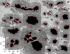 |
Fig. 1 Selection of the analysed sample of sunspots displayed on the same scale. The white contours mark the intensity threshold of 50% of the quiet-Sun intensity. The red contours are independently defined and outline isocontours of 1867 G of Bver . Only contours encircling regions larger than 3 Mm2 are shown. Sunspots marked (L) clearly show a systematic displacement of the white and red contours that is due to line-of-sight effects. Sunspots marked (U) have regions where the red contours lie within the intensity (white) contours. The arrows point to the disc centre. The numbers denote the heliocentric angle of the sunspot. |
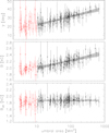 |
Fig. 2 Mean values of the magnetic field inclination (A), the magnetic field strength (B), and the vertical component of the magnetic field (C) for every identified boundary as a function of the area encircled by the given boundary. The uncertainties represent the standard deviations of the physical parameters at the boundaries. Contours encircling areas smaller than 10 Mm2 marked in red are not considered for the statistical analyses. The dashed line corresponds to the most probable value estimated by a Bayesian linear regression, and the shaded area denotes the 99% confidence interval of the estimated model. |
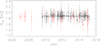 |
Fig. 3 Dependence of Bver on the phase of the solar cycle. Contours encircling areas smaller than 10 Mm2 and sunspots observed in solar cycle 23 are marked in red and not considered for the statistical analyses. The dashed line corresponds to the most probable value estimated by a Bayesian linear regression, and the shaded area denotes the 99% confidence interval of the estimated model. |
4 Discussion and conclusions
While in stable sunspots the intensity and the Bver boundary contours are coupled, cases are also observed in which the Bver = 1867 G isocontour lies within the intensity contour (see sunspots marked U in Fig. 1 and Jurčák et al. 2015, 2017). We conjecture that the empirical law presented here serves as a stability criterion in evolving spots and proto-spots: pores and umbral areas with Bver higher than 1867 G are stable, while umbral areas with lower Bver are unstable. That is to say, they are prone to be transformed into a different mode of magneto-convection like a penumbra or light bridges. This is also why we restricted our statistical analysis to umbral areas larger than 10 Mm2. Smaller areas are typically observed to be in a transient state.
Moreover, light bridges harbour horizontal magnetic fields (Beckers & Schröter 1969; Jurčák et al. 2006; Felipe et al. 2016). We find that our empirical law indeed applies here as well, as demonstrated in the examples shown in Fig. 1. Based on images of very high spatial resolution, Schlichenmaier et al. (2016) reported that the fine structure in the boundary of light bridges is found to share morphological aspects with the inner boundary of penumbral filaments, suggesting that the modes of magneto-convection in light bridges and penumbrae are coupled to the umbral mode in a similar manner.
The implications of these findings have profound consequences on the formation process of the penumbra. While the umbra harbours strong vertical fields (Bray & Loughhead 1964; Solanki 2003), horizontal fields are the essential property of penumbral filaments (Tiwari et al. 2013; Jurčák et al. 2014). During the formation of the penumbra, the umbral magnetic field with sufficiently low Bver is converted into a penumbral magnetic field (Jurčák et al. 2015, 2017).
There must therefore exist a mechanism that turns vertical (umbral) fields into horizontal (penumbral) fields. An explanation of this process regulated by the interplay between the convective and magnetic forces seems straightforward, but is fundamentally new: from the convectively unstable sub-photosphere, hot buoyant plasma pushes upwards along the umbral field lines. When cooling, the mass load exerted by the plasma will bend and incline the field lines of a reduced (lower than 1867 G) vertical field. Only in strong vertical magnetic fields (higher than 1867 G) is the magnetic tension as a restoring force strong enough to prevent the field lines from bending over and becoming horizontal. This scenario is consistent with the fallen flux tube model by Wentzel (1992) and with numerical simulations of the penumbral fine structure, which showed that the mass load in inclined penumbral field lines overcomes the magnetic tension to form a horizontal penumbral filament (Rempel 2011).
The discovery of the empirical law defining the existence of a critical vertical component of the magnetic field governing the umbra boundary in stable sunspots solves the long-standing question on the nature of this boundary, and it gives fundamental new insights into the magneto-convective modes of energy transport in sunspots, which will be addressed in following studies.
Acknowledgements
The authors wish to thank I. Thaler for fruitful discussions and A. Asensio Ramos for apreliminary Bayesian analysis of the data. J.J. acknowledges the support from RVO:67985815. R.R. acknowledges financial support by the DFG grant RE 3282/1-1 and by the Spanish Ministry of Economy and Competitiveness through project AYA2014-60476-P. N.B.G. acknowledges financial support by the Senatsausschuss of the Leibniz-Gemeinschaft, Ref.-No. SAW-2012-KIS-5 within the framework of the CASSDA project. Hinode is a Japanese mission developed and launched by ISAS/JAXA, with NAOJ as domestic partner and NASA and STFC (UK) as international partners. It is operated by these agencies in cooperation with ESA and NSC (Norway).
Appendix A Datasets
In Table A.1 we summarise all the datasets that were used for the statistical analysis. For each listed item in Table A.1, we constructed a continuum intensity map with marked intensity isocontours at 50% of the local quiet-Sun intensity and isocontours at Bver = 1867 G. These maps are shown in Fig. A.1. When the date, time, and NOAA numbers were identical in Table A.1, the scan was separated into sub-fields for display purposes.
List of Hinode SP scans.
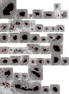 |
Fig. A.1 Hinode SP maps. The spatial scale in all panels is the same, with one tick mark of the axis being 1′′. The white contours mark the intensity threshold of 50% of the quiet-Sun intensity. The red contours are independently defined and outline the isocontours of 1867 G of Bver. Only contours encircling regions larger than 3 Mm2 are shown. The arrows point to the disc centre. The black numbers denote the heliocentric angle of the sunspot. The red numbers refer to the scan number as listed in Table A.1. |
We performed both a Bayesian linear regression and a standard linear regression. Before we performed these statistical analyses, we centred and scaled the x values of each explanatory variable to ensure better numerical stability:
 where μ(x) is the mean of the explanatory variable, and σ(x) is the standard deviation of the explanatory variable.
Appendix B Statistical analysis
B. 1 Bayesian linear regression
The inference with the Bayesian linear model can be found in standard textbooks (Denison et al. 2002). We assumed conjugate priors. These assumptions imply that the marginal prior distributions of the regression parameters are the multivariate t-distributions and the square of the standard deviation of the dependent variable error (σ2) follows the inverse gamma distribution. The parameters of the marginal posterior distributions can be computed analytically and follow the same standard distributions as priors.
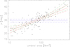 |
Fig. B.1 Scatter plot showing the dependence of magnetic field inclination on the umbra area. A black cross marks the observed data points. The line colour denotes the model complexity of the Bayesian linear regression; blue shows a constant model, red a linear model, and green a quadratic model. The solid lines mark the most probable value estimated by the corresponding model, and the dashed lines mark the 99% confidence interval of the estimated model. |
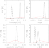 |
Fig. B.5 Prior (red lines) and posterior (black lines) distributions of the regression coefficients and standard deviation of the error distribution for the dependence of magnetic field inclination on the logarithm of the area. The solid lines correspond to the constant model, the dashed lines to the linear model, and the dash-dotted lines to the quadratic model. |
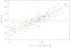 |
Fig. B.9 Scatter plot showing the dependence of the magnetic field inclination on the umbra area. Black crosses mark the observed data points. The line colour denotes the model complexity of the standard linear regression; blue shows a constant model, red a linear model, and green a quadratic model. The solid lines mark the best fit, and the dashed lines mark the 99% confidence interval of the estimated model. |
Bayes factors for the magnetic field inclination as a function of the area logarithm.
Bayes factors for the magnetic field strength as a function of the area logarithm.
Bayes factors for the Bver as a function of the area logarithm.
Bayes factors for the Bver as a function of the phase of solar cycle 24.
Model parameters for γ as a function of the area logarithm.
Model parameters for B as a function of the area logarithm.
Model parameters for Bver as a function of the area logarithm.
We used the following parameter values:
-
for noise of the dependent variable Bver, we set the parameters of the inverse gamma distribution to obtain the mode of the marginal prior distribution of σ, which is about 145 G, which corresponds to the value estimated from the observed data,
-
for noise of the dependent variable B, we set the parameters of the inverse gamma distribution to obtain the mode of the marginal prior distribution of σ, which is about 165 G, which corresponds to the value estimated from the observed data,
-
for noise of the dependent variable γ, we set the parameters of the inverse gamma distribution to obtain the mode of the marginal prior distribution of σ, which is about 5 deg, which corresponds to the value estimated from the observed data,
-
the prior distributions of the intercept values of γ, B, and Bver have a mean corresponding to the mean value of the observed data of each of the dependent variable, and the t-distribution is scaled by the standard deviation of the error of the dependent variables,
-
the prior distributions of the slope values of γ, B, and Bver have a mean of zero to eliminate any preferences, and the distributions are scaled by the standard deviation,
-
the prior distributions of the quadratic coefficients of γ, B, and Bver have a mean of zero to eliminate any preferences, and the distributions are scaled by the standard deviation.
The results of Bayesian linear regression are shown in Figs. B.1–B.3. The most likely solutions and the 99% confidence intervals presented in these figures are derived from the resulting posterior distributions that are shown in Figs. B.5–B.8. The prior and posterior distributions of the regression parameters are presented using the scaled and centred explanatory variables.
For every learned model M, we computed the marginal log-likelihood of the model and compared the constant model (M0), the linear model (M1), and the quadratic model (M2) using the Bayes factors (BF), which is defined as the ratio of marginal likelihoods of the two compared models. We summarise the results in Tables B.1–B.4. The hypothesis for each element of the matrix is in favour of the model associated with the row against the model associated with the column. A widely used interpretation (Jeffreys 1961) of the strength of evidence for Bayes factor B is the following:
-
BF ≤ 0.1 – strong against,
-
0.1 < BF ≤ 1∕3 – substantial against,
-
1∕3 < BF < 1 – barely worth mentioning against,
-
1 ≤ BF < 3 – barely worth mentioning for,
-
3 ≤ BF < 10 – substantial for,
-
10 ≤ BF – strong for.
We can draw the following conclusions from Tables B.1–B.4 and Figs. B.1–B.8:
-
There is strong evidence in the data that the magnetic field inclination is not constant and is a function of the logarithm of the area. The resulting confidence intervals do not allow us to distinguish if the dependence of γ on the logarithm of the area is linear or quadratic.
-
There is strong evidence in the data that the strength of the magnetic field is not constant and is a function of the logarithm of the area. The resulting confidence intervals do not allow us to distinguish if the dependence of B on the logarithm of the area is linear or quadratic.
-
There isno substantial evidence in the data that the vertical component of the magnetic field is a linear or a quadratic function of the logarithm of the area. The constantsolution is well within the confidence intervals of the linear and quadratic solutions.
-
There isno substantial evidence in the data that the vertical component of the magnetic field is a linear or a quadratic function of the date. The constant solution is well within the confidence intervals of the linear and quadratic solutions.
Figures B.1–B.3 show that the 99% confidence intervals of the estimated models are quite narrow compared to the spread of the measured values of dependent variables. This can be explained by the fact that the Bayesian analysis allows splitting the overall uncertainty between the uncertainty of model parameters (which we see in these figures) and the error represented by the value of the standard deviation (see the bottom right plots in Figs. B.5–B.8).
B.2 Standard linear regression
The goal of the standard linear regression (Weisberg 2005) is to estimate the vector of the linear regression coefficients β from the measured data. We estimated the coefficients by solving the linear least-squares problem using the QR factorization. Each coefficient is a normally distributed random variable. For each coefficient we report
-
its value,
-
the standard error of each coefficient, which is the standard deviation of its distribution. It measures the uncertainty in the estimate of the coefficient,
-
its p-value, which is the probability of achieving the same or a higher value of the t-statistics if the null hypothesis were true. The null hypothesis is that the corresponding value of β is zero. Ifthe p-value was higher than 0.01, we did not reject the null hypothesis. The p-value was computed for the coefficients learned from the scaled and centred data.
For each model we also report the p-value, that is, the probability of achieving a value of the t-statistics as high or higher if the null hypothesis were true, where the null hypothesis is the intercept-only model. If the p-value was higher than 0.01, we did not reject the null hypothesis. With this p-value, the probability of incorrectly rejecting a true null hypothesis is typically close to 15% (Sellke et al. 2001).
The resulting values of standard linear regression are listed in Tables B.5–B.8. These values are used to plot the best fit and the 99% confidence intervals in Figs. B.9–B.12.
Model parameters for Bver as a function of the phase of solar cycle 24.
The results of the standard linear regression are in full agreement with the results of the Bayesian linear regression:
-
There is strong evidence in the data that the magnetic field inclination is not constant and is a function of the logarithm of the area as the p-values of both linear and quadratic models are extremely low and we can reject the constant model.
-
There is strong evidence in the data that the strength of the magnetic field is not constant and is a function of the logarithm of the area as the p-values of both linear and quadratic models are extremely low and we can reject the constant model.
-
There is no substantial evidence in the data that the vertical component of the magnetic field is a linear or a quadratic function of the logarithm of the area. The p-values of the more complex models are above 0.01, that is, we cannot reject the constant model.
-
There is no substantial evidence in the data that the vertical component of the magnetic field is a linear or a quadratic function of the date. The p-values of the linear and quadratic models are above 0.01, meaning that we cannot reject the constant model.
References
- Balthasar, H., & Collados, M. 2005, A&A, 429, 705 [NASA ADS] [CrossRef] [EDP Sciences] [Google Scholar]
- Balthasar, H., & Schmidt, W. 1993, A&A, 279, 243 [NASA ADS] [Google Scholar]
- Beck, C. 2008, A&A, 480, 825 [NASA ADS] [CrossRef] [EDP Sciences] [Google Scholar]
- Beckers, J. M., & Schröter, E. H. 1969, Sol. Phys., 10, 384 [NASA ADS] [CrossRef] [Google Scholar]
- Bellot Rubio, L. R., Balthasar, H., & Collados, M. 2004, A&A, 427, 319 [NASA ADS] [CrossRef] [EDP Sciences] [Google Scholar]
- Borrero, J. M., & Ichimoto, K. 2011, Liv. Rev. Sol. Phys., 8, 4 [Google Scholar]
- Borrero, J. M., Solanki, S. K., Bellot Rubio, L. R., Lagg, A., & Mathew, S. K. 2004, A&A, 422, 1093 [NASA ADS] [CrossRef] [EDP Sciences] [Google Scholar]
- Bray, R. J., & Loughhead, R. E. 1964, Sunspots, (London: Chapman and Hall) [Google Scholar]
- Denison, D., Holmes, C., Mallick, B., & Smith, A. 2002, Bayesian Methods for Nonlinear Classification and Regression (Wiley) [Google Scholar]
- Felipe, T., Collados, M., Khomenko, E., et al. 2016, A&A, 596, A59 [NASA ADS] [CrossRef] [EDP Sciences] [Google Scholar]
- Hale, G. E. 1908, ApJ, 28, 315 [Google Scholar]
- Jeffreys, H. 1961, The Theory of Probability, 3rd edn. (Oxford University Press) [Google Scholar]
- Jurčák, J. 2011, A&A, 531, A118 [NASA ADS] [CrossRef] [EDP Sciences] [Google Scholar]
- Jurčák, J., Martínez Pillet, V., & Sobotka, M. 2006, A&A, 453, 1079 [NASA ADS] [CrossRef] [EDP Sciences] [Google Scholar]
- Jurčák, J., Bellot Rubio, L. R., & Sobotka, M. 2014, A&A, 564, A91 [NASA ADS] [CrossRef] [EDP Sciences] [Google Scholar]
- Jurčák, J., Bello González, N., Schlichenmaier, R., & Rezaei, R. 2015, A&A, 580, L1 [NASA ADS] [CrossRef] [EDP Sciences] [Google Scholar]
- Jurčák, J., Bello González, N., Schlichenmaier, R., & Rezaei, R. 2017, A&A, 597, A60 [NASA ADS] [CrossRef] [EDP Sciences] [Google Scholar]
- Keppens, R., & Martinez Pillet, V. 1996, A&A, 316, 229 [NASA ADS] [Google Scholar]
- Kosugi, T., Matsuzaki, K., Sakao, T., et al. 2007, Sol. Phys., 243, 3 [NASA ADS] [CrossRef] [Google Scholar]
- Lites, B. W., & Ichimoto, K. 2013, Sol. Phys., 283, 601 [NASA ADS] [CrossRef] [Google Scholar]
- Lites, B. W., Skumanich, A., & Scharmer, G. B. 1990, ApJ, 355, 329 [NASA ADS] [CrossRef] [Google Scholar]
- Lites, B. W., Low, B. C., Martínez Pillet, V., et al. 1995, ApJ, 446, 877 [NASA ADS] [CrossRef] [Google Scholar]
- Mathew, S. K., Lagg, A., Solanki, S. K., et al. 2003, A&A, 410, 695 [NASA ADS] [CrossRef] [EDP Sciences] [Google Scholar]
- Pevtsov, A. A., Bertello, L., Tlatov, A. G., et al. 2014, Sol. Phys., 289, 593 [Google Scholar]
- Rempel, M. 2011, ApJ, 729, 5 [NASA ADS] [CrossRef] [Google Scholar]
- Rezaei, R., Beck, C., & Schmidt, W. 2012, A&A, 541, A60 [NASA ADS] [CrossRef] [EDP Sciences] [Google Scholar]
- Rezaei, R., Beck, C., Lagg, A., et al. 2015, A&A, 578, A43 [NASA ADS] [CrossRef] [EDP Sciences] [Google Scholar]
- Ruiz Cobo, B., & del Toro Iniesta, J. C. 1992, ApJ, 398, 375 [NASA ADS] [CrossRef] [Google Scholar]
- Sánchez Cuberes, M., Puschmann, K. G., & Wiehr, E. 2005, A&A, 440, 345 [NASA ADS] [CrossRef] [EDP Sciences] [Google Scholar]
- Schad, T. A. 2014, Sol. Phys., 289, 1477 [NASA ADS] [CrossRef] [Google Scholar]
- Schlichenmaier, R., von der Lühe, O., Hoch, S., et al. 2016, A&A, 596, A7 [NASA ADS] [CrossRef] [EDP Sciences] [Google Scholar]
- Sellke, T., Bayarri, M. J., & Berger, J. O. 2001, Am. Stat., 55, 62 [CrossRef] [Google Scholar]
- Solanki, S. K. 2003, A&ARv, 11, 153 [Google Scholar]
- Solanki, S. K., & Montavon, C. A. P. 1993, A&A, 275, 283 [NASA ADS] [Google Scholar]
- Solanki, S. K., Rüedi, I., & Livingston, W. 1992, A&A, 263, 339 [NASA ADS] [Google Scholar]
- Tiwari, S. K., van Noort, M., Lagg, A., & Solanki, S. K. 2013, A&A, 557, A25 [NASA ADS] [CrossRef] [EDP Sciences] [Google Scholar]
- Tsuneta, S., Ichimoto, K., Katsukawa, Y., et al. 2008, Sol. Phys., 249, 167 [NASA ADS] [CrossRef] [Google Scholar]
- Weisberg, S. 2005, Applied Linear Regression, 3rd edn. (Wiley) [CrossRef] [Google Scholar]
- Wentzel, D. G. 1992, ApJ, 388, 211 [NASA ADS] [CrossRef] [Google Scholar]
- Westendorp Plaza C., del Toro Iniesta, J. C., Ruiz Cobo, B., et al. 2001, ApJ, 547, 1130 [NASA ADS] [CrossRef] [Google Scholar]
All Tables
Bayes factors for the magnetic field inclination as a function of the area logarithm.
Bayes factors for the magnetic field strength as a function of the area logarithm.
All Figures
|
Fig. 1 Selection of the analysed sample of sunspots displayed on the same scale. The white contours mark the intensity threshold of 50% of the quiet-Sun intensity. The red contours are independently defined and outline isocontours of 1867 G of Bver . Only contours encircling regions larger than 3 Mm2 are shown. Sunspots marked (L) clearly show a systematic displacement of the white and red contours that is due to line-of-sight effects. Sunspots marked (U) have regions where the red contours lie within the intensity (white) contours. The arrows point to the disc centre. The numbers denote the heliocentric angle of the sunspot. |
| In the text | |
|
Fig. 2 Mean values of the magnetic field inclination (A), the magnetic field strength (B), and the vertical component of the magnetic field (C) for every identified boundary as a function of the area encircled by the given boundary. The uncertainties represent the standard deviations of the physical parameters at the boundaries. Contours encircling areas smaller than 10 Mm2 marked in red are not considered for the statistical analyses. The dashed line corresponds to the most probable value estimated by a Bayesian linear regression, and the shaded area denotes the 99% confidence interval of the estimated model. |
| In the text | |
|
Fig. 3 Dependence of Bver on the phase of the solar cycle. Contours encircling areas smaller than 10 Mm2 and sunspots observed in solar cycle 23 are marked in red and not considered for the statistical analyses. The dashed line corresponds to the most probable value estimated by a Bayesian linear regression, and the shaded area denotes the 99% confidence interval of the estimated model. |
| In the text | |
|
Fig. A.1 Hinode SP maps. The spatial scale in all panels is the same, with one tick mark of the axis being 1′′. The white contours mark the intensity threshold of 50% of the quiet-Sun intensity. The red contours are independently defined and outline the isocontours of 1867 G of Bver. Only contours encircling regions larger than 3 Mm2 are shown. The arrows point to the disc centre. The black numbers denote the heliocentric angle of the sunspot. The red numbers refer to the scan number as listed in Table A.1. |
| In the text | |
|
Fig. B.1 Scatter plot showing the dependence of magnetic field inclination on the umbra area. A black cross marks the observed data points. The line colour denotes the model complexity of the Bayesian linear regression; blue shows a constant model, red a linear model, and green a quadratic model. The solid lines mark the most probable value estimated by the corresponding model, and the dashed lines mark the 99% confidence interval of the estimated model. |
| In the text | |
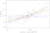 |
Fig. B.2 Same as Fig. B.1, but for the dependence of Bver on the umbral area. |
| In the text | |
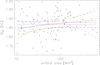 |
Fig. B.3 Same as Fig. B.1, but for the dependence of Bver on the phase of solar cycle 24. |
| In the text | |
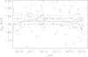 |
Fig. B.4 Same as Fig. B.1, but for the dependence of the magnetic field strength on the umbral area. |
| In the text | |
|
Fig. B.5 Prior (red lines) and posterior (black lines) distributions of the regression coefficients and standard deviation of the error distribution for the dependence of magnetic field inclination on the logarithm of the area. The solid lines correspond to the constant model, the dashed lines to the linear model, and the dash-dotted lines to the quadratic model. |
| In the text | |
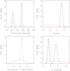 |
Fig. B.6 Same as Fig. B.5, but for the dependence of B on the logarithm of the area. |
| In the text | |
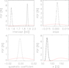 |
Fig. B.7 Same as Fig. B.5, but for the dependence of Bver on the logarithm of the area. |
| In the text | |
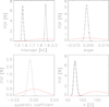 |
Fig. B.8 Same as Fig. B.5, but for the dependence of Bver on the phase of solar cycle 24. |
| In the text | |
|
Fig. B.9 Scatter plot showing the dependence of the magnetic field inclination on the umbra area. Black crosses mark the observed data points. The line colour denotes the model complexity of the standard linear regression; blue shows a constant model, red a linear model, and green a quadratic model. The solid lines mark the best fit, and the dashed lines mark the 99% confidence interval of the estimated model. |
| In the text | |
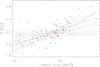 |
Fig. B.10 Same as Fig. B.9, but for the dependence of B on the logarithm of the umbral area. |
| In the text | |
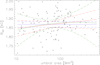 |
Fig. B.11 Same as Fig. B.9, but for the dependence of Bver on the logarithm of the umbral area. |
| In the text | |
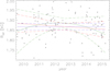 |
Fig. B.12 Same as Fig. B.9, but for the dependence of Bver on the phase of solar cycle 24. |
| In the text | |
Current usage metrics show cumulative count of Article Views (full-text article views including HTML views, PDF and ePub downloads, according to the available data) and Abstracts Views on Vision4Press platform.
Data correspond to usage on the plateform after 2015. The current usage metrics is available 48-96 hours after online publication and is updated daily on week days.
Initial download of the metrics may take a while.