| Issue |
A&A
Volume 611, March 2018
|
|
|---|---|---|
| Article Number | A26 | |
| Number of page(s) | 11 | |
| Section | Astrophysical processes | |
| DOI | https://doi.org/10.1051/0004-6361/201731861 | |
| Published online | 20 March 2018 | |
Charge exchange in galaxy clusters
1
RIKEN Nishina Center,
2-1 Hirosawa,
Wako,
Saitama 351-0198,
Japan
e-mail: This email address is being protected from spambots. You need JavaScript enabled to view it.
2
SRON Netherlands Institute for Space Research,
Sorbonnelaan 2,
3584 CA Utrecht,
The Netherlands
3
Leiden Observatory, Leiden University,
PO Box 9513,
2300 RA Leiden,
The Netherlands
4
Astronomical Institute “Anton Pannekoek”,
Science Park 904, University of Amsterdam,
1098 XH Amsterdam,
The Netherlands
5
Max-Planck-Institut für Kernphysik,
Heidelberg,
69117 Heidelberg,
Germany
Received:
30
August
2017
Accepted:
13
October
2017
Abstract
Context. Though theoretically expected, the charge exchange emission from galaxy clusters has never been confidently detected. Accumulating hints were reported recently, including a rather marginal detection with the Hitomi data of the Perseus cluster. As previously suggested, a detection of charge exchange line emission from galaxy clusters would not only impact the interpretation of the newly discovered 3.5 keV line, but also open up a new research topic on the interaction between hot and cold matter in clusters.
Aim. We aim to perform the most systematic search for the O VIII charge exchange line in cluster spectra using the RGS on board XMM-Newton.
Methods. We introduce a sample of 21 clusters observed with the RGS. In order to search for O VIII charge exchange, the sample selection criterion is a >35σ detection of the O VIII Lyα line in the archival RGS spectra. The dominating thermal plasma emission is modeled and subtracted with a two-temperature thermal component, and the residuals are stacked for the line search. The systematic uncertainties in the fits are quantified by refitting the spectra with a varying continuum and line broadening.
Results. By the residual stacking, we do find a hint of a line-like feature at 14.82 Å, the characteristic wavelength expected for oxygen charge exchange. This feature has a marginal significance of 2.8σ, and the average equivalent width is 2.5 × 10⁻⁴ keV. We further demonstrate that the putative feature can be barely affected by the systematic errors from continuum modeling and instrumental effects, or the atomic uncertainties of the neighboring thermal lines.
Conclusions. Assuming a realistic temperature and abundance pattern, the physical model implied by the possible oxygen line agrees well with the theoretical model proposed previously to explain the reported 3.5 keV line. If the charge exchange source indeed exists, we expect that the oxygen abundance could have been overestimated by 8−22% in previous X-ray measurements that assumed pure thermal lines. These new RGS results bring us one step forward to understanding the charge exchange phenomenon in galaxy clusters.
Key words: atomic processes / line: identification / techniques: spectroscopic / galaxies: clusters: intracluster medium
© ESO 2018
1 Introduction
Charge exchange (CX) occurs when a neutral atom collides with a sufficiently charged ion, and recombines the ion into a highly excited state. It is the dominant atomic process at the interface where the highly charged solar wind interacts with comet atmospheres (Lisse et al. 1996; Cravens 1997). X-ray observations showed that the solar wind CX also influences planet atmospheres and the heliosphere (Snowden et al. 2004; Dennerl et al. 2006; Fujimoto et al. 2007; Branduardi-Raymont et al. 2007; Smith et al. 2014). Although the observation of CX from extrasolar objects is still quite challenging, there are a growing number of reports for possible CX from supernova remnants (Katsuda et al. 2011), starburst galaxies (Tsuru et al. 2007; Liu et al. 2011), active galactic nuclei (Gu et al. 2017), and galaxy clusters (Fabian et al. 2011; Gu et al. 2015; Hitomi Collaboration et al. 2017).
Among these objects, the possible CX from galaxy clusters has recently attracted more attention because it becomes intimately related with the interpretation of a newly discovered potential X-ray line at ~3.5 keV. As reported in Bulbul et al. (2014), Boyarsky et al. (2014), and more recently in Cappelluti et al. (2017), a weak line feature at ~3.5 keV is detected in the spectra of a large sample of galaxies and clusters observed by XMM-Newton EPIC and Chandra ACIS. It could not be identified immediately in the standard line tables of thermal plasma. These authors thus considered it to be a truly exceptional feature, and proposed that it might stem from particle physics: the radiative decay of a dark matter candidate called a sterile neutrino. However, in Gu et al. (2015), we showed that there might be a missing element in their atomic model: the charge exchange in the hot intracluster medium (ICM). The observed residual at ~3.5 keV with the X-ray CCDs would be washed away (or reduced to within 1σ) by introducing the CX-excited S XVI line at ~3.45 keV. Our atomic calculation has been verified recently by a dedicated laboratory measurement (Shah et al. 2016).
Not only the physical interpretation, but also the detection of the 3.5 keV line itself is still in controversy. So far all the detections have been made by X-ray CCDs with spectral resolution of ~100 eV. The putative line is then blurred into a 1% bump above the continuum, affected easily by instrumental and atomic uncertainties. Resolving the feature with a high-resolution spectrometer is therefore essential. The calorimeter on board the Hitomi satellite provides a resolution of ~5 eV at the target energy, offering such an opportunity for the first time. As reported in Hitomi Collaboration et al. (2017), the Hitomi Perseus data can rule out, at least at 99%, an unidentified line at the flux level reported in the previous XMM-Newton and Chandra studies, even though the Hitomi data were a bit shallow in the target energy band. Interestingly, it does show a hint of the S XVI CX line at ~3.45 keV. By analyzing the Hitomi data in more detail, a hint was discovered of the Fe XXV CX line at ~8.78 keV (Hitomi Collaboration et al., in prep.), and the upper limits of the sulfur and iron line fluxes are well in line with the model prediction in Gu et al. (2015).
The Hitomi results open up a new window for CX astrophysics. The possible CX signal from galaxy clusters provides a new approach to locating the cold matter and to investigating its interaction with the hot ICM. To confirm the Hitomi results, we carry out a systematic CX line search using the existing cluster data obtained with the XMM-Newton Reflection Grating Spectrometer (RGS), which offers a high resolving power of 150− 700 for soft X-ray lines from galaxy clusters. We aim to achieve the most stringent constraint on the CX phenomenon in clusters using cutting-edge high-resolution X-ray spectrometers. This paper is structured as follows. First, we determine the target CX line by a theoretical calculation in Sect. 2. Then in Sects. 3 and 4, we present the target selection and data reduction. Section 5 describes the analysis and shows the results based on the RGS sample. The physical implications of the observed results are presented in Sect. 6, and summarized in Sect. 7. Throughout the paper, the errors are given at a 68% confidence level.
2 Target charge exchange line
This work aims to search for CX signatures using the RGS instrument, which already limits the candidate elements to be C, N, O, Ne, Mg, Fe, and Ni. For the ICM, C and N are hard to detect, and the wavelengths of the Mg XII CX lines (~6.4 Å) are too close to the bandpass limit. For the Fe and Ni L-shell lines (mostly Li-like to Na-like sequences), the theoretical calculations for CX cross sections are still lacking, even though there are a few laboratory measurements (Beiersdorfer et al. 2008). The best candidate thus becomes O, which is generally much more abundant than Ne. We would focus on O VIII recombined from proton-like oxygen ions, which are the most abundant species of oxygen ions in the ICM.
To determine the target emission feature, we calculate the CX lines using the cx model in SPEX version 3.03.00 (Gu et al. 2016a), and compare them with the emission in collisional ionization equilibrium (CIE; Fig. 1). The model plasma has a temperature of 2 keV and solar abundance. We assume CX collisions between bare oxygenand hydrogen atoms at a velocity of 500 km s−1. When normalizing the CX and CIE lines at the Lyα transitions, the only significant difference appears at the Lyδ (1s−5p) lines at ~14.82 Å. This occurs because electron capture into atomic levels with principal quantum number n = 5 is dominant for the adopted collision condition. In fact, according to the theoretical calculation by, e.g., Janev et al. (1993), n = 5 remains as the peak capture channel for a collision velocity ≤4000 km s−1, which means that the O VIII Lyδ transitions would be the key CX signature in most of the relevant astrophysical conditions. A more recent n-resolved multichannel Landau-Zener calculation by Mullen et al. (2017) shows the same peak at n = 5 for a similar velocity range.
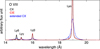 |
Fig. 1 CX (black) and CIE (red) O VIII lines convolved with the RGS response. The plasma temperature is set to 2 keV, and the collision velocity for CX is 500 km s−1 . The two models are normalized at the Lyα line. The blue curve shows the CX lines further broadened by the spatial extent of a representative cluster (2A 0335). |
3 Sample selection
The cluster sample is selected using three criteria. First, the targets must show significant O VIII Lyα lines. A quick filtering is done by scanning through the standard RGS spectra archived in the BiRD catalog1 and pickingup spectra with O VIII Lyα lines that can be identified by eye. Then we extract the RGS spectra of candidates (see the data reduction in Sect. 5), and determine the O VIII Lyα line significance by fitting the restframe 0.62−0.69 keV band with two Gaussians representing Lyα1 and Lyα2, and the line-free CIE model for the continuum. Then we selected objects with O VIII Lyα line significance higher than 5σ. This reduces the catalog to a list of 49 objects, which forms the “preliminary sample”.
Second, the nearby M87 and Perseus cluster are removed from the sample because of their oversized angular extents that blur the target line and reduce the detection sensitivity. There are now 47 objects remaining in the list, which we call the “intermediate sample”.
The third criterion is to exclude objects with strong Fe XVII emission lines. The Fe XVII line at 15.02 Å is a close neighbor to the target O VIII Lyδ line at 14.82 Å, so that the astrophysical and instrumental broadening of the Fe line might potentially affect the detection of the O line. Using the updated ionization equilibrium balance calculation in SPEX 3.03.00 (Urdampilleta et al. 2017), we find that the absolute concentration of Fe XVII becomes negligible (<10−10) at a balance temperature of 1.8 keV, which is then set as the final criterion for the sample. We check the average temperatures reported in Pinto et al. (2015) and keep objects with temperatures higher than 1.8 keV. This reduces the “intermediate sample” to the final sample of 21 objects. The properties of the 21 objects are listed in Table 1.
XMM-Newton RGS data of the sample clusters.
4 Data
We process the XMM-Newton RGS and MOS data, mostly following the method described in Pinto et al. (2015). The MOS data are not used for spectral analysis, but for determining the spatial extent of the source along the dispersion direction of the RGS.
The data reduction is done with the SAS version 16.0.0 and the latest calibration files. The SAS tasks rgsproc and emproc are run for the RGS and MOS data, respectively. The time intervals contaminated by soft-proton are detected using the light curves of the RGS CCD9, which are then filtered by a 2σclipping. To search extensively for the CX signal, the width of the RGS source extraction region (xpsfincl) is set to 99% of the point spread function, which is approximately a 3.4 arcmin belt centered on the emission peak. The modeled background spectra are used in the spectral analysis. The diffuse cosmic background is not modeled explicitly, since it is smeared out and merged into the continuum. The spectral files are converted to SPEX format through the SPEX task trafo.
To model the spectral broadening due to the spatial extent of the sources, we extract the MOS1 image in the 0.5−1.8 keV band for each observation, and calculate the surface brightness profile in the RGS dispersion direction using the rgsvprof task in SPEX. The spectral broadening is then modeled using the SPEX model lpro based on the brightness profiles. The line broadening can be further fine-tuned by varying the scale parameter s of the lpro model, which is left free in the fitting.
We analyze the first- and second-order RGS spectra in the 8−28 Å band. All abundances are relative to Lodders & Palme (2009) proto-solar standard. We use optimally binned spectra by the obin command in SPEX (Kaastra & Bleeker 2016), and C-statistics for fitting and error estimation. We adopt the updated ionization balance calculations of Urdampilleta et al. (2017).
5 Spectral analysis and results
We aim to search for a weak line feature at 14.82 Å, which means that the dominant thermal emission must be properly modeled and subtracted. Here we carry out two approaches, the global and local fits, to model the thermal emission. The global fit uses a full self-consistent calculation of line and continuum emission to fit the entire band, and the local fit calculates the sum of a simple continuum plus a series of Gaussian emission lines to model a narrow band near the target line. The latter method might provide a better representation of the local continuum, while it cannot model all the weak lines, especially the thermal O VIII Lyδ component at the target wavelength. Thus the two approaches would compensate each other. Combined global and local fits were also used in other recent X-ray work, e.g., Mernier et al. (2016).
5.1 Global fits
To describe the cluster thermal component, we fit the spectra using two SPEX cie models because our sample is built up from mostly cool-core clusters, which are known to show both hot- and cool- phase ICM in the cores (Gu et al. 2012). The emission measures and electron temperatures of the hot and cool components are left to vary, while the N, O, Ne, Mg, Fe, and Ni abundances of the two cie components are coupled to each other. The ion temperatures are tied to the electron temperatures. The two-temperature model is modified first by a redshift component, then by a hot model for foreground absorption. The absorber is neutral (kT = 0.5 eV), has solar abundances, and its column density is set to the calculated value from Willingale et al. (2013), which includes the contribution from both atomic and molecular components. Finally, the two-temperature model is multiplied by the lpro component to correct for the spatial broadening of the objects (Sect. 4). All the spectra in our sample can be modeled with pure thermal emission; none of them requires an additional power-law spectral component for the AGN. The same treatment was also used in Pinto et al. (2015) and de Plaa et al. (2017). This does not necessarily mean that AGNs are absent, but merely that the thermal components are apparently dominant in these spectra. The global fit of the RGS spectrum of Abell 85 is shown in Fig. 2 as an example.
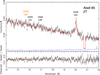 |
Fig. 2 Example RGS first-order spectrum of Abell 85. The best-fit two-temperature model is shown in red, and the subtracted instrumental background is plotted in blue. The target O VIII Lyδ feature is indicated in orange. |
To measure the intensity of the possible weak line at 14.82 Å, we add a Gaussian component with a fixed wavelength in the fits. The Gaussian line is multiplied by the same redshift and absorption components as those applied to the thermal model. The spatial distribution of the possible charge exchange component is unclear; it might be emitted mostly from the cluster core or significantly contributed by the cool gas in member galaxies. In the former case, a point source PSF would be adequate for the line, while in the latter case the Gaussian should be multiplied by the lpro component of the entire cluster (Fig. 1). In Fig. 3, we show the best-fit results for both cases.
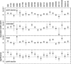 |
Fig. 3 Best-fit equivalent widths of a Gaussian component at rest-frame wavelength of 14.82 Å, based on both the global and local fits of the thermal component. For the global fits, the Gaussian line PSF is set to both the point source and extended source modes. By dividing the best-fit equivalent width (global fits/point source) by their errors, the line significance for each cluster is shown in the bottom panel. |
5.2 Local fits
To search for the target weak line, it is crucial to model the continuum and related thermal line to high precision. Although the global fits can describe the target band reasonably well, it might still be affected by the calibration imperfections of the RGS instrument (de Vries et al. 2015), the uncertainties in atomic code(Mernier et al. 2017), and astrophysical complexity (de Plaa et al. 2017). These effects can be corrected by fitting the spectra locally, using a model including sufficient freedom to account for the thermal emission and the associated errors. The local fit is based on a model including a single-temperature cie continuum by setting ions ignore all in SPEX, together with a set of Gaussian components with fixed central energies for the strong thermal lines. The local fit is carried out in the 13–23 Å band, and the added thermal emission lines are listed in Table 2. The continuum and Gaussian lines are multiplied first by the redshift and hot components, and then by the lpro for the spatial broadening. Another narrow Gaussian component is added at the cluster-frame wavelength of 14.82 Å to account for the CX line. This approach is essentially the same as the one used in recent weak line detection works (e.g., Bulbul et al. 2014).
Emission lines included in the local fits.
The average C-statistics with the local fit is improved from the global fit by about 10 for ~300 degrees of freedom. Although useful for obtaining a better approximation to the 13−23 Å band, the local method misses details from the global modeling of the full spectrum; for instance, the weak emission lines, such as the thermal O VIII Lyδ line, are ignored. The equivalent widths of the CX line obtained with the local fits must thus be treated as the upper limit.
5.3 Results
We calculate the equivalent widths of the Gaussian component at rest-frame 14.82 Å, based on the best fits from both global and local approaches. For the global fit, we further derive the equivalent widths for both point- and extended-source approximations. If the target line does not exist, the sample should show positive and negative equivalent widths to be equally distributed around zero. As shown in Fig. 3, the best-fit equivalent widths are clearly more seen on the positive side. The results using three methods (global/point source, global/extended source, and local/point source) agree well with each other, and none of the sources has a significantly negative line flux at 14.82 Å. By dividing thebest-fit equivalent widths by their errors, we further plot the significance in Fig. 3. It shows that all the seeming excesses at 14.82 Å are ≤2σ significance;most objects are consistent with 1σ. Although there is a hint of a line at the target wavelength, this means that it is not possible to report a significant detection in any individual object.
This naturally leads us to a stacking approach for better statistics. Here we blue-shift all the residual spectra to the source frame, and average them with a weighting based on the counts in each energy bin. The residual spectra for each object are obtained using the two-temperature, single-temperature, and local fit modelings. The Gaussian component at 14.82 Å is excluded forthe stacking. In Fig. 4, we plot the stacked residual spectra in the 13.4 Å to 17.4 Å band. The total stacking exposure is about 2.4 Ms. To examine instrumental effects, we also show the residual plot based on the RGS2 data alone, as well as the plot without redshift correction. The latter is apparently dominated by instrumental artifacts; by comparing it with the first three residuals in Fig. 4, it is clear that the instrumental effects are smeared out by the redshift correction, while the features with cluster origin should stay.
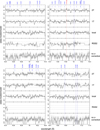 |
Fig. 4 Stacked residuals in the rest-frame 13.4–17.4 Å band. Different panels show the residuals from the two-temperature/single-temperature global fits and the local fits, the residuals by RGS2 data alone, and the residuals stacked without redshift correction. The dashed lines show a5% level. |
The stacked residuals of the two-temperature, single-temperature, and local fit modelings are in general agreement with each other. The amplitudes of the residuals are mostly within 5% of the model value; at 14.82 Å, all the three stacked plots consistently show a line-like excess, with a peak value of 3−4%. By fitting the residual with a Gaussian line in the 14.8–14.85 Å band, the significance of the target feature is obtained to be 3.1σ, 2.8σ, and 3.4σ with the two-temperature, single-temperature, and local modelings, respectively. The Gaussian line has a best-fit sigma of 0.03−0.04 Å, which agrees with a narrow line feature broadened purely by the instrument (RGS FWHM = 0.06−0.07 Å at the target wavelength). This feature can be seen using the RGS2 data alone, and the intensity is consistent with the RGS1+2 results, suggesting that it is unlikely to be an artifact on one of the two detectors. This is further supported by the residual spectrum stacked before the redshift correction, in which no apparent instrumental feature (such as gaps) near the target wavelength is seen.
Several other features are revealed in Fig. 4. The thermal Fe XVII lines at rest-frame 15.02 Å, 15.26 Å, 16.78 Å, 17.05 Å, and 17.10 Å are seen in the stacked residual based on single-temperature modeling; all the four lines are found at the correct wavelengths, indicating that the wavelength of the target feature at 14.82 Å should also be accurate. The weak Fe XVII features are at least partially modeled out by the two-temperature fit. This occurs because the Fe XVII lines must be emitted from the cool phase ICM (kT < 1.5 keV), which is accounted for by the two-temperature model.
To be conservative, the stacked significance of the target line is 2.8σ (single-temperature fit), which means a marginal detection. Since the wavelength of the target line is well-defined by atomic theory, and is accurately measured by experiments (Beiersdorfer et al. 2003), there is no look-elsewhere effect (Gross & Vitells 2010) in the detection significance. As shown in Table 3, the weighted average of the equivalent widths derived from the global fits is 2.5 × 10⁻⁴ keV, with an upper limit of 3.4 × 10⁻⁴ keV. The detection of the putative feature might still be affected byseveral systematic uncertainties and biases, which will be studied in the following section.
Weighted means of the best-fit equivalent widths.
5.4 Systematic effects
5.4.1 Bias due to instrumental and astrophysical modeling
The background component and AGN power-law emission do not play a major role, since we focus on the brightest core of clusters where the ICM emission dominates in the RGS band. As shown in Fig. 2, the typical instrumental background component at the target energy is just a small percent of the cluster emission. The background spectrum is nearly featureless in the plot. Such continuum components are hence unlikely to create any significant sharp feature at the target wavelength of 14.82 Å.
Anotherpossible uncertainty in the continuum modeling is the column density (NH) of the absorbing Galactic ISM. The current NH values are fixed to the total Galactic hydrogen column (H I + H2) published inWillingale et al. (2013). However, it is reported that the NH measured with the X-ray data of galaxy clusters sometimes deviate from the Galactic hydrogen column. This might be partly due to the calibration uncertainties in the X-ray instruments and errors in the solar abundance table (Schellenberger et al. 2015; de Plaa et al. 2017). How does a potential NH error affect the spectral fitting at the target wavelength 14.82 Å?
To test the effect of NH uncertainty, we perform a new two-temperature fit to each object by allowing its NH to vary freely. The Gaussian component at 14.82 Å is excluded in the fits. The best-fit NH values distribute around the Galactic values with a standard deviation of about 1020 cm2 . We then shift the best-fit residuals to the source frame, and stack them in the same way as in Sect. 5.3. In Fig. 5, we show that for a narrow band 14.4–15.4 Å, the stacked residual with the free NH agrees well with the original residual with fixed NH , and the possible CX feature remains intact with the varying absorption.
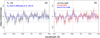 |
Fig. 5 Panel a: stacked residuals in the rest-frame 14.4–15.4 Å band, yielded by fits with NH free values (black) and with NH values of Willingale et al. (2013; blue). Panel b: results from the global fits with line broadening fixed to half (black) andtwo times (red) the best-fit value. The blue plot is the same as shown in Fig. 4. |
Since RGS is a non-slit spectrometer, the spectral lines are broadened by the spatial extent of the source. For thermal plasma, it is determined by the projected emission measure distribution of the respective ion. Since the distributions of ions in a cluster might sometimes be different (de Plaa et al. 2006), the resulting line widths thus differ for different elements. However, the current standard spectral analysis tool cannot fit each element independently; it gives only an average line width (Sect. 4). The potential deviation between the average and the true width of strong emission lines might induce residuals mostly at the wing of the lines. The question is whether or not this might explain the observed putative feature at 14.82 Å.
To address the effect of line broadening, we force the line width to be a factor of two smaller/larger than the original values, and rerun the global fits for each object. The line width change is achieved by fixing the scale parameter s to be twice/half of the best-fit values obtained in the original fits. In this way, the broadening profile varies by a total factor of four, which is roughly consistent with the observed discrepancy between the O VIII and Fe lines reported in de Plaa et al. (2006). Following Sect. 5.3, we then blue-shift the new residuals obtained from the global fits to z = 0, and stack them weighted by the counts. As shown in Fig. 5, the two stacked residuals with scaled line broadening are in good agreement with each other at 14.4−15.4 Å, and the positive residuals peaked at 14.82 Å can be seen at the same level as the original fits. This means that the line broadening has little effect on the fits of the target band. This is probably owing to the lack of strong emission lines near 15 Å for the selected clusters.
5.4.2 Bias due to atomic data errors
Although the target O VIII CX line is relatively well isolated in the spectra of hot clusters, it still has some neighboring weak lines. Could the putative feature at 14.82 Å come from atomic data errors in the normal thermal emission? Here we investigate the atomic uncertainties of the adjacent thermal lines. For the selected high-temperature clusters in our sample, there are only weak thermal lines, mainly from Fe XX and O VIII, in the proximity of the target CX line.
Fe XX might emit two satellite lines at 14.824 Å and 14.849 Å, from the transitions of 2s2p4 4P5∕2–2s22p2(3P)3p 4D7∕2 and 2s2p4 4P5∕2–2s22p2(3P)3p 2D3∕2, respectively. To address the atomic uncertainties, we compare the line emissivities in SPEX v3.03 and APEC v3.0.8. Figure 6 plots the SPEX and APEC fluxes of these two satellite lines, scaled to the main Fe XX line at 14.283 Å from 2s2p4 4P5∕2–2s2p3(5S)3s 4S3∕2 transition, as a function of the balance temperature. The relative differences between SPEX and APEC, which can be approximated as the atomic uncertainties, are <65% for the 14.824 Å line and <50% for the 14.849 Å line. In the same figure, we show that line fluxes in both SPEX and APEC are much lower than 1% of the local continuum. Though uncertain, these two satellite lines are apparentlytoo weak to give any significant feature on the RGS spectrum.
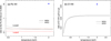 |
Fig. 6 Panel a: model line ratios of Fe XX 14.849 Å (black) and 14.824 Å (red) to the main transition at 14.283 Å, calculated by the thermal model in SPEX v3.03 (solid) and APEC v3.0.8 (dashed). Panel b: O VIII Lyδ to Lyα ratio as a function of temperature for the two thermal codes. The blue points in both figures show the value required to create a 1% excess above the continuum at 14.82 Å for a 2 keV plasma. |
The atomic error associated with the O VIII Lyδ line emitted from thermal plasma also contributes to the systematic uncertainties. Here we compare the calculations by the CIE model in SPEX v3.03 and APEC v3.0.8. Figure 6 shows the total O VIII Lyδ doublet fluxes normalized to the Lyα lines as a function of the balance temperature. The relative differences between SPEX and APEC are <4% at 0.1 keV and 5% at 2 keV. To create a line feature of 1% of the local continuum, the O VIII Lyδ flux must be underestimated by a factor of >2, which is much larger than the difference between SPEX and APEC. Hence, the thermal O VIII lines are quite accurate, and the induced systematic error to the target energy band is quite small.
6 Discussion
Using the high-resolution spectroscopic data for a sample of massive galaxy clusters, we report a marginal detection of a charge exchange feature at 14.82 Å created by fully ionized oxygen interacting with neutral matter. Although the feature is weak, it cannot be easily explained either by the systematic uncertainties due to continuum modeling and instrumental broadening or by the atomic uncertainties of the adjacent thermal emission lines. The new CX feature poses a series of questions to be answered: (i) what is the origin of the possible CX emission? (ii) is the new O VIII line consistent with the CX scenario proposed for the possible 3.5 keV line? and (iii) how does it potentially affect the previous measurements of the ICM abundance based on pure thermal modeling?
6.1 Origin of the charge exchange emission
Given the observed line profile and the derived parameters, it is likely that the CX emission originates from the cold gas clouds embedded in the hot ICM. The foreground solar wind charge exchange in the geocorona/heliosphere is negligible since it can hardly form a line in the RGS spectrum, due to the instrumental broadening.
The cold gas clouds are often observed near the central galaxies in clusters (Conselice et al. 2001), and/or in the wake of the member galaxies during their infall (Gu et al. 2013a,b; Yagi et al. 2015; Gu et al. 2016b). Since these neutral structures are completely immersed in the pool of highly ionized plasma, the CX process is thus naturally expected at the interface, strongly affecting the ionization state of the interface. To investigate the possible relation between the CX and the cold clouds, in Fig. 7 we compare the best-fit normalization of the Gaussian component at 14.82 Å for each cluster with its Hα luminosity measured with the VLT spectroscopic data (Hamer et al. 2016). The Hα data was chosen because it illustrates the excitation (or recombination) process of the cold clouds, which might occur at a similar location as the CX. The plot shows that we can hardly conclude any significant relation between the possible CX and Hα emission based on the current sample and data quality; a further study with deeper X-ray data is needed. One potential bias on the plot is that the Hα data includeonly the central galaxies, while the RGS data might also be affected by the CX associated with the member galaxies in its field of view.
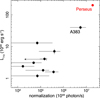 |
Fig. 7 Measured normalizations of the Gaussian line at 14.82 Å plotted against the Hα line luminosities taken from Hamer et al. (2016). As a reference, we also plot the expected O VIII Lyδ line strength for the Perseus cluster, estimated based on the CX model that best fits the Hitomi data (Hitomi Collaboration et al., in prep.). A solar abundance ratio is assumed since the Hitomi spectrum does not cover the oxygen band. The Hα luminosity of the Perseus cluster is taken from Conselice et al. (2001). |
6.2 Charge exchange model
Here we provide a physical model for the possible O VIII CX line. The CX flux is given by
 (1)where Dl is the luminosity distance of the object, nI and nN are respectively the densities of ionized and neutral media, v is the collision velocity, V is the interaction volume, and σI, N is the charge exchange cross section as a function of the velocity v and the energy of the capture state characterized primarily by the quantum numbers n, l, and S. The cross section calculation is described in Gu et al. (2016a). By defining emission measure as ∫ nInNdV , we show in Fig. 8 the model calculation of equivalent width of O VIII Lyδ line as a function of emission measure for a collision velocity v varying in the range of 50−800 km s−1. The thermal component used in the calculation is taken from the best-fit two-temperature model of Abell 85 (Fig. 2). The ionization temperature and abundances of the CX component are assumed to be the same as the thermal plasma. To give the sample-average equivalent width of 2.5 × 10⁻⁴ keV at 14.82 Å, the CX component would have an emission measure ranging from 4 × 1067 cm−3 for v = 50 km s−1 to 3 × 1066 cm−3 for v = 800 km s−1. Assuming an ICM density of ~5 × 10⁻² cm−3 at cluster cores (Zhuravleva et al. 2014) and a neutral gas density of ~10 cm−3 in the molecular clouds (Heiner et al. 2008), the effective interaction volume is then ~5−15 kpc3.
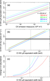 |
Fig. 8 Panel a: equivalent width of the O VIII Lyδ line as a function of the CX emission measure for different collision velocities, calculated based on the cx model in SPEX. The background thermal component is taken from the best-fit two-temperature model for Abell 85. The observed sample-averaged equivalent width is shown by a dashed line in all panels. Panel b: model calculation of S XVI CX line flux at ~3.5 keV as a function of O VIII Lyδ equivalent width. The shadow region shows the observed flux of the unidentified 3.5 keV line in Bulbul et al. (2014). Panel c: fractional change in oxygen abundance as a function of O VIII Lyδ equivalent width. The color schemes in panels b and c are the same as in panel a. |
The estimated CX emission measure is generally consistent with the predicted value in Gu et al. (2015). The theoretical model in Gu et al. (2015) is proposed to explain a possible weak emission line at ~3.5 keV from galaxy clusters reported in Bulbul et al. (2014) and Boyarsky et al. (2014), by a CX reaction between bare sulfur ions and neutral atoms. It is hence naturally expected that the detections at the 3.5 keV and 14.82 Å would boil down to the same CX source. To prove this, we plot in Fig. 8 the model calculation of the S XVI flux at ~3.5 keV as a function of the O VIII Lyδ equivalent width for different v. The sulfur ions are assumed to have the same ionization temperature and abundance as the oxygen ions. For the same O VIII equivalent width, the 3.5 keV flux increases with the collision velocity for v < 300 km s−1, and decreases with velocity for larger v. This occurs because the CX capture spreads into more adjacent atomic levels of the sulfur ions at high velocity, and hence the line at 3.5 keV smears out. For the model yielding the O VIII equivalent width of 2.5 × 10⁻⁴ keV, the predicted S XVI line flux at ~3.5 keV is 3.5−6.5 × 10⁻⁶ photons cm−2 s−1, which agrees well with the observed value reported in Bulbul et al. (2014). This clearly shows that the possible O VIII CX line is well in line with the model in Gu et al. (2015) for the possible ~3.5 keV line.
Here wecompare our results with a previous work by Walker et al. (2015). By analyzing the stacked Chandra CCD data of the X-ray/Hα filaments in the Perseus cluster, Walker et al. (2015) found that the X-ray spectra can be well fit with a CX component for the emissionfrom the filament surface together with a thermal component from the surrounding ICM. They reported a CX flux of ~1.3 × 10⁻¹³ ergs cm−2 s−1 in the 0.5−1.0 keV band, 57% of the total X-ray flux from the filament regions. This value is lower, by a factor of 5, than our estimate of the average CX flux in the same band based on Eq. (1) andthe observed equivalent width of O VIII Lyδ line. The difference might be explained by at least two factors: the selection of X-ray/Hα filaments in Walker et al. (2015) is far from complete (see their Fig. 1), and the CX model used in their work (Smith et al. 2012)clearly differs from the one in our study (Gu et al. 2016a).
Walker et al. (2015) also presented an XMM-Newton RGS spectrum of the Centaurus cluster, showing a lack of significant oxygen lines predicted by their CX model. This is not surprising since the CX features, if they exist, are indeed rather weak in all objects of our sample (Fig. 3), it must be difficult to report a significant detection based on the data from any individual cluster.
6.3 Effect on ICM abundance measurement
For such a newly proposed component with a relatively weak spectral feature, the CX emission is often ignored in the ICM analysis. If the CX component does exist, it should have introduced a bias on the abundance measurement as it produces strong Lyα lines which blend with the thermal lines. By analyzing the Hitomi data of the Perseus cluster, Hitomi Collaboration et al. (in prep.) suggested that the Fe abundance is overestimated by ~5% if the CX component is ignored in the fits. To estimate the possible impact on the oxygen abundance, we simulate the CX + CIE spectrum in SPEX, and fit it with a pure CIE model. The input CIE model is taken from the best-fit model of Abell 85, multiplied by the observed line broadening profile. The input CX model has the same ionization balance and abundances as the CIE component. As shown in Fig. 8, for the input CX O VIII equivalent width of 2.5 × 10⁻⁴ keV, the best-fit CIE abundance becomes higher than the input value by ~8−22% for v = 100−800 km s−1. It shows that the model predicts a higher Lyα/Lyδ ratio for a larger collision velocity. As reported in de Plaa et al. (2017), the measurement uncertainty on the oxygen abundance by the same RGS data of Abell 85 is 12%. This indicates that the bias on the ICM abundance caused by the possible CX component is marginally significant for the current instruments.
This simulation is based on an object with a temperature of 3−4 keV, and shows the typical level of systematic difference in abundance to expect. In real clusters with different temperatures, or if the spatial distribution of the CX component becomes very different from the thermal ICM, the effects on the abundance measurement will be different. The impact on other elements is expected to be comparable or relatively smaller.
The CX lines are calculated using the theoretical cross sections reported in Janev et al. (1993). As shown in Gu et al. (2017), the different theoretical approaches might sometimes differ quite a lot from each other, yielding a large systematic error on the line ratios. The laboratory data needed to verify the atomic codes are not at all complete. When instead the results from multi-channel Landau-Zener method in Mullen et al. (2017) are used, the O VIII Lyα/Lyδ ratio decreases by 70% at v = 100 km s−1, which would hence lead to a further larger systematic difference on the oxygen abundance.
The possible charge exchange emission from diffuse astrophysical objects will be much better measured with future calorimeter missions. In Fig. 9, we show the simulated XARM and Athena spectra at the O VIII Lyδ band. The input model consisting of the best-fit thermal model for Abell 85, and a CX component giving an equivalent width of 2.5 × 10⁻⁴ keV at 14.82 Å, is convolved with the XARM and Athena responses and fitted with apure thermal model. The excess at 14.82 Å is detected at 5σ for an exposure of 200 ks with the Athena X-IFU. This indicates that to characterize the charge exchange process in the intracluster space, we will need high spectral resolution spectra from telescopes with a large effective area. For the XARM spectrum, detecting the CX using the O VIII line alone becomes much more difficult; clearly, we also have to investigate the CX features at other energies, such as the S XVI at ~3.5 keV and the Fe XXV at ~8.8 keV, and those reported in Hitomi Collaboration et al. (in prep.) and Hitomi Collaboration et al. (2017). A more systematic simulation on the CX astrophysics with future X-ray missions will be presented in an upcoming paper.
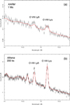 |
Fig. 9 Simulated 1 Ms XARM and 200 ks Athena spectra of CIE + CX emission from an Abell 85-type object fitted by a CIE model alone. |
7 Conclusion
We perform a systematic search for a charge exchange emission line at the rest-frame wavelength of 14.82 Å in a RGS sample of 21 galaxy clusters. The line is a characteristic feature that indicates strong physical interaction between bare oxygen ions and neutral particles. By fitting the thermal component and stacking the residuals, we find a hint of a line-like feature at the target wavelength. The possible feature has a 2.8σ significance above the local thermal component, corresponding to an average equivalent width of 2.5 × 10⁻⁴ keV. Although it only constitutes a marginal detection, it cannot be easily accounted for by either instrumental effects or atomic uncertainties. If it is indeed a CX line from galaxy clusters, it would indicate exactly the same physical model as the one reported in Gu et al. (2015), which was proposed to explain an unidentified line found earlier at ~3.5 keV. The model is also well in line with the possible CX component marginally detected with the Hitomi spectrum of the Perseus cluster. Although the CX emission is expected to be weak, it implies a potential overestimation of the oxygen abundance by 8−22% in previous abundance measurements. A confirmation of this feature has to wait for spectroscopic observations with a future mission of higher sensitivity.
Acknowledgments
L.G. acknowledges financial support from the RIKEN/SPDR program. SRON is supported financially by NWO, the Netherlands Organization for Scientific Research.
References
- Beiersdorfer, P., Boyce, K. R., Brown, G. V., et al. 2003, Science, 300, 1558 [NASA ADS] [CrossRef] [PubMed] [Google Scholar]
- Beiersdorfer, P., Schweikhard, L., Liebisch, P., & Brown, G. V. 2008, ApJ, 672, 726 [NASA ADS] [CrossRef] [Google Scholar]
- Boyarsky, A., Ruchayskiy, O., Iakubovskyi, D., & Franse, J. 2014, Phys. Rev. Lett., 113, 251301 [NASA ADS] [CrossRef] [PubMed] [Google Scholar]
- Branduardi-Raymont, G., Bhardwaj, A., Elsner, R. F., et al. 2007, A&A, 463, 761 [NASA ADS] [CrossRef] [EDP Sciences] [Google Scholar]
- Bulbul, E., Markevitch, M., Foster, A., et al. 2014, ApJ, 789, 13 [NASA ADS] [CrossRef] [Google Scholar]
- Cappelluti, N., Bulbul, E., Foster, A., et al. 2017, ApJ, submitted, ArXiv e-prints [Google Scholar]
- Conselice, C. J., Gallagher, III, J. S., & Wyse, R. F. G. 2001, AJ, 122, 2281 [NASA ADS] [CrossRef] [Google Scholar]
- Cravens, T. E. 1997, Geophys. Res. Lett., 24, 105 [NASA ADS] [CrossRef] [Google Scholar]
- de Plaa, J., Werner, N., Bykov, A. M., et al. 2006, A&A, 452, 397 [NASA ADS] [CrossRef] [EDP Sciences] [Google Scholar]
- de Plaa, J., Kaastra, J. S., Werner, N., et al. 2017, A&A, 607, A98 [NASA ADS] [CrossRef] [EDP Sciences] [Google Scholar]
- de Vries, C. P., den Herder, J. W., Gabriel, C., et al. 2015, A&A, 573, A128 [NASA ADS] [CrossRef] [EDP Sciences] [Google Scholar]
- Dennerl, K., Lisse, C. M., Bhardwaj, A., et al. 2006, A&A, 451, 709 [NASA ADS] [CrossRef] [EDP Sciences] [Google Scholar]
- Fabian, A. C., Sanders, J. S., Williams, R. J. R., et al. 2011, MNRAS, 417, 172 [NASA ADS] [CrossRef] [Google Scholar]
- Fujimoto, R., Mitsuda, K., Mccammon, D., et al. 2007, PASJ, 59, 133 [NASA ADS] [Google Scholar]
- Gross, E., & Vitells, O. 2010, Eur. Phys. J. C, 70, 525 [NASA ADS] [CrossRef] [EDP Sciences] [Google Scholar]
- Gu, L., Xu, H., Gu, J., et al. 2012, ApJ, 749, 186 [NASA ADS] [CrossRef] [Google Scholar]
- Gu, L., Gandhi, P., Inada, N., et al. 2013a, ApJ, 767, 157 [NASA ADS] [CrossRef] [Google Scholar]
- Gu, L., Yagi, M., Nakazawa, K., et al. 2013b, ApJ, 777, L36 [NASA ADS] [CrossRef] [Google Scholar]
- Gu, L., Kaastra, J., Raassen, A. J. J., et al. 2015, A&A, 584, L11 [NASA ADS] [CrossRef] [EDP Sciences] [Google Scholar]
- Gu, L., Kaastra, J., & Raassen, A. J. J. 2016a, A&A, 588, A52 [NASA ADS] [CrossRef] [EDP Sciences] [Google Scholar]
- Gu, L., Wen, Z., Gandhi, P., et al. 2016b, ApJ, 826, 72 [NASA ADS] [CrossRef] [Google Scholar]
- Gu, L., Mao, J., O’Dea, C. P., et al. 2017, A&A, 601, A45 [NASA ADS] [CrossRef] [EDP Sciences] [Google Scholar]
- Hamer, S. L., Edge, A. C., Swinbank, A. M., et al. 2016, MNRAS, 460, 1758 [NASA ADS] [CrossRef] [Google Scholar]
- Heiner, J. S., Allen, R. J., Emonts, B. H. C., & van der Kruit, P. C. 2008, ApJ, 673, 798 [NASA ADS] [CrossRef] [Google Scholar]
- Hitomi Collaboration, Aharonian, F. A., Akamatsu, H., Akimoto, F et al. 2017, ApJ, 837, L15 [NASA ADS] [CrossRef] [Google Scholar]
- Janev, R. K., Phaneuf, R. A., Tawara, H., & Shirai, T. 1993, Atomic Data and Nuclear Data Tables, 55, 201 [NASA ADS] [CrossRef] [Google Scholar]
- Kaastra, J. S., & Bleeker, J. A. M. 2016, A&A, 587, A151 [NASA ADS] [CrossRef] [EDP Sciences] [Google Scholar]
- Katsuda, S., Tsunemi, H., Mori, K., et al. 2011, ApJ, 730, 24 [NASA ADS] [CrossRef] [Google Scholar]
- Lisse, C. M., Dennerl, K., Englhauser, J., et al. 1996, Science, 274, 205 [NASA ADS] [CrossRef] [EDP Sciences] [Google Scholar]
- Liu, J., Mao, S., & Wang, Q. D. 2011, MNRAS, 415, L64 [NASA ADS] [CrossRef] [Google Scholar]
- Lodders, K., & Palme, H. 2009, Meteoritics and Planetary Science Supplement, 72, 5154 [Google Scholar]
- Mernier, F., de Plaa, J., Pinto, C., et al. 2016, A&A, 592, A157 [NASA ADS] [CrossRef] [EDP Sciences] [Google Scholar]
- Mernier, F., de Plaa, J., Kaastra, J. S., et al. 2017, A&A, 603, A80 [NASA ADS] [CrossRef] [EDP Sciences] [Google Scholar]
- Mullen, P. D., Cumbee, R. S., Lyons, D., et al. 2017, ApJ, 844, 7 [NASA ADS] [CrossRef] [Google Scholar]
- Pinto, C., Sanders, J. S., Werner, N., et al. 2015, A&A, 575, A38 [NASA ADS] [CrossRef] [EDP Sciences] [Google Scholar]
- Schellenberger, G., Reiprich, T. H., Lovisari, L., Nevalainen, J., & David, L. 2015, A&A, 575, A30 [NASA ADS] [CrossRef] [EDP Sciences] [Google Scholar]
- Shah, C., Dobrodey, S., Bernitt, S., et al. 2016, ApJ, 833, 52 [NASA ADS] [CrossRef] [Google Scholar]
- Smith, R. K., Foster, A. R., & Brickhouse, N. S. 2012, Astron. Nachr., 333, 301 [NASA ADS] [CrossRef] [Google Scholar]
- Smith, R. K., Foster, A. R., Edgar, R. J., & Brickhouse, N. S. 2014, ApJ, 787, 77 [NASA ADS] [CrossRef] [Google Scholar]
- Snowden, S. L., Collier, M. R., & Kuntz, K. D. 2004, ApJ, 610, 1182 [NASA ADS] [CrossRef] [Google Scholar]
- Tsuru, T. G., Ozawa, M., Hyodo, Y., et al. 2007, PASJ, 59, 269 [NASA ADS] [Google Scholar]
- Urdampilleta, I., Kaastra, J. S., & Mehdipour, M. 2017, A&A, 601, A85 [NASA ADS] [CrossRef] [EDP Sciences] [Google Scholar]
- Walker, S. A., Kosec, P., Fabian, A. C., & Sanders, J. S. 2015, MNRAS, 453, 2480 [NASA ADS] [Google Scholar]
- Willingale, R., Starling, R. L. C., Beardmore, A. P., Tanvir, N. R., & O’Brien, P. T. 2013, MNRAS, 431, 394 [NASA ADS] [CrossRef] [Google Scholar]
- Yagi, M., Gu, L., Koyama, Y., et al. 2015, AJ, 149, 36 [NASA ADS] [CrossRef] [Google Scholar]
- Zhuravleva, I., Churazov, E., Schekochihin, A. A., et al. 2014, Nature, 515, 85 [Google Scholar]
All Tables
All Figures
|
Fig. 1 CX (black) and CIE (red) O VIII lines convolved with the RGS response. The plasma temperature is set to 2 keV, and the collision velocity for CX is 500 km s−1 . The two models are normalized at the Lyα line. The blue curve shows the CX lines further broadened by the spatial extent of a representative cluster (2A 0335). |
| In the text | |
|
Fig. 2 Example RGS first-order spectrum of Abell 85. The best-fit two-temperature model is shown in red, and the subtracted instrumental background is plotted in blue. The target O VIII Lyδ feature is indicated in orange. |
| In the text | |
|
Fig. 3 Best-fit equivalent widths of a Gaussian component at rest-frame wavelength of 14.82 Å, based on both the global and local fits of the thermal component. For the global fits, the Gaussian line PSF is set to both the point source and extended source modes. By dividing the best-fit equivalent width (global fits/point source) by their errors, the line significance for each cluster is shown in the bottom panel. |
| In the text | |
|
Fig. 4 Stacked residuals in the rest-frame 13.4–17.4 Å band. Different panels show the residuals from the two-temperature/single-temperature global fits and the local fits, the residuals by RGS2 data alone, and the residuals stacked without redshift correction. The dashed lines show a5% level. |
| In the text | |
|
Fig. 5 Panel a: stacked residuals in the rest-frame 14.4–15.4 Å band, yielded by fits with NH free values (black) and with NH values of Willingale et al. (2013; blue). Panel b: results from the global fits with line broadening fixed to half (black) andtwo times (red) the best-fit value. The blue plot is the same as shown in Fig. 4. |
| In the text | |
|
Fig. 6 Panel a: model line ratios of Fe XX 14.849 Å (black) and 14.824 Å (red) to the main transition at 14.283 Å, calculated by the thermal model in SPEX v3.03 (solid) and APEC v3.0.8 (dashed). Panel b: O VIII Lyδ to Lyα ratio as a function of temperature for the two thermal codes. The blue points in both figures show the value required to create a 1% excess above the continuum at 14.82 Å for a 2 keV plasma. |
| In the text | |
|
Fig. 7 Measured normalizations of the Gaussian line at 14.82 Å plotted against the Hα line luminosities taken from Hamer et al. (2016). As a reference, we also plot the expected O VIII Lyδ line strength for the Perseus cluster, estimated based on the CX model that best fits the Hitomi data (Hitomi Collaboration et al., in prep.). A solar abundance ratio is assumed since the Hitomi spectrum does not cover the oxygen band. The Hα luminosity of the Perseus cluster is taken from Conselice et al. (2001). |
| In the text | |
|
Fig. 8 Panel a: equivalent width of the O VIII Lyδ line as a function of the CX emission measure for different collision velocities, calculated based on the cx model in SPEX. The background thermal component is taken from the best-fit two-temperature model for Abell 85. The observed sample-averaged equivalent width is shown by a dashed line in all panels. Panel b: model calculation of S XVI CX line flux at ~3.5 keV as a function of O VIII Lyδ equivalent width. The shadow region shows the observed flux of the unidentified 3.5 keV line in Bulbul et al. (2014). Panel c: fractional change in oxygen abundance as a function of O VIII Lyδ equivalent width. The color schemes in panels b and c are the same as in panel a. |
| In the text | |
|
Fig. 9 Simulated 1 Ms XARM and 200 ks Athena spectra of CIE + CX emission from an Abell 85-type object fitted by a CIE model alone. |
| In the text | |
Current usage metrics show cumulative count of Article Views (full-text article views including HTML views, PDF and ePub downloads, according to the available data) and Abstracts Views on Vision4Press platform.
Data correspond to usage on the plateform after 2015. The current usage metrics is available 48-96 hours after online publication and is updated daily on week days.
Initial download of the metrics may take a while.