| Issue |
A&A
Volume 611, March 2018
|
|
|---|---|---|
| Article Number | A16 | |
| Number of page(s) | 14 | |
| Section | Interstellar and circumstellar matter | |
| DOI | https://doi.org/10.1051/0004-6361/201731347 | |
| Published online | 16 March 2018 | |
Sulphur monoxide exposes a potential molecular disk wind from the planet-hosting disk around HD 100546
1
School of Physics and Astronomy, University of Leeds,
Leeds
LS2 9JT, UK
e-mail: This email address is being protected from spambots. You need JavaScript enabled to view it.
, This email address is being protected from spambots. You need JavaScript enabled to view it.
2
Institute of Astronomy,
Madingley Rd,
Cambridge
CB3 0HA, UK
3
Harvard-Smithsonian Center for Astrophysics,
60 Garden Street,
Cambridge,
MA
02138, USA
4
Leiden Observatory, Leiden University,
PO Box 9513,
2300 RA
Leiden, The Netherlands
Received:
9
June
2017
Accepted:
12
December
2017
Abstract
Sulphur-bearing volatiles are observed to be significantly depleted in interstellar and circumstellar regions. This missing sulphur is postulated to be mostly locked up in refractory form. With ALMA we have detected sulphur monoxide (SO), a known shock tracer, in the HD 100546 protoplanetary disk. Two rotational transitions: J = 77–66 (301.286 GHz) and J = 78–67 (304.078 GHz) are detected in their respective integrated intensity maps. The stacking of these transitions results in a clear 5σ detection in the stacked line profile. The emission is compact but is spectrally resolved and the line profile has two components. One component peaks at the source velocity and the other is blue-shifted by 5 km s−1. The kinematics and spatial distribution of the SO emission are not consistent with that expected from a purely Keplerian disk. We detect additional blue-shifted emission that we attribute to a disk wind. The disk component was simulated using LIME and a physical disk structure. The disk emission is asymmetric and best fit by a wedge of emission in the north-east region of the disk coincident with a “hot-spot” observed in the CO J = 3–2 line. The favoured hypothesis is that a possible inner disk warp (seen in CO emission) directly exposes the north-east side of the disk to heating by the central star, creating locally the conditions to launch a disk wind. Chemical models of a disk wind will help to elucidate why the wind is particularly highlighted in SO emission and whether a refractory source of sulphur is needed. An alternative explanation is that the SO is tracing an accretion shock from a circumplanetary disk associated with the proposed protoplanet embedded in the disk at 50 au. We also report a non-detection of SO in the protoplanetary disk around HD 97048.
Key words: astrochemistry / submillimeter: planetary systems / stars: individual: HD 100546, HD 97048 / protoplanetary disks / stars: pre-main sequence
© ESO 2018
1 Introduction
Investigating the chemical structure and evolution of protoplanetary disks is important when studying planet formation as the composition of a planet is determined by the content of its parent disk. The physical and chemical conditions in disks can be traced with observations of molecular line emission (see Henning & Semenov 2013; Dutrey et al. 2014, and references therein). These observations are key to understanding disk chemistry resulting from changes in disk structure due to planet-disk interactions.
Transition disks were the first disks identified to possess signatures of clearing by unseen planets (Strom et al. 1989). Protoplanet candidates have been identified in the cavities of some transition disks e.g. LkCa 15 (Sallum et al. 2015) and HD 169142 (Reggiani et al. 2014). These disks are expected to have a rich observable chemistry due to the disk midplane being directly exposed to far-UV radiation from the central star. Molecules that otherwise would be frozen out onto grains in the cold, shielded midplane of the disk may be detectable (Cleeves et al. 2011). High spatial resolution observations with ALMA allow investigation into the physical and chemical conditions associated with planet-forming regions of nearby disks.
The dominant volatiles (gas and ice) in protoplanetary disks are composed of hydrogen, oxygen, carbon, nitrogen and sulphur. Sulphur is observed to be significantly depleted in circumstellar regions with detections of gas-phase S-bearing molecules accounting for ~0.1% only of the estimated cosmic abundance (Tieftrunk et al. 1994; Dutrey et al. 1997; Ruffle et al. 1999). The missing sulphur is thought to reside in or on the solid dust grains in the disk, the most abundant molecule being H2S in cometary ices (Bockelée-Morvan et al. 2000) and also in iron sulphides, another main component of primitive comets and meteorites (Keller et al. 2002). The lack of agreement between observed abundances and chemical models points towards as yet unaccounted for grain-surface processes preventing desorption of H2S and the formation of gas phase S-bearing species (Dutrey et al. 2011). This is supported by non-detections of anticipated molecules despite deep targeted searches in young stellar objects (e.g., Martín-Doménech et al. 2016).
Despite the depletion issue, sulphur-bearing species are useful tracers of physical processes in interstellar and circumstellar material. For example, SO is frequently detected as a tracer of shocked gas associated with the bipolar outflows from Class 0 and I protostars (e.g., Tafalla et al. 2010; Podio et al. 2015; Sakai et al. 2016). Searches for SO have found that detections in outflows are ubiquitous but in protoplanetary disks infrequent (Guilloteau et al. 2013). The first detection of SO in a circumstellar disk was reported by Fuente et al. (2010). They observed the J = 34–23 (138.178 GHz) transition in the transitional disk around AB Aur. This detection was confirmed by Pacheco-Vázquez et al. (2015) with detections of the higher frequency J = 54–43 (206.176 GHz) and J = 56–45 (219.949 GHz) transitions. Further observations and modelling suggest that the SO is distributed in a ring (145 to 384 au) and is depleted in the region of the disk’s horse-shoe shaped dust trap (Pacheco-Vázquez et al. 2016). Most recently, Guilloteau et al. (2016) report the detection of the SO J = 65–54 (251.826 GHz) and J = 67–56 (261.844 GHz) transitions in four disks out of 30 that were observed with the IRAM 30-m telescope. The aforementioned studies show that SO has been detected in both T Tauri and Herbig disks. ALMA observations have also revealed ring components of SO emission in Class 0 protostars (Ohashi et al. 2014; Podio et al. 2015; Sakai et al. 2016) that have been interpreted as accretion shocks at the disk-envelope interface.
It is evident from existing observations that SO is a tracer of shocks in Class 0 and I protostars. However, SO is an elusive disk molecule requiring high sensitivity observations for its detection: this is now possible with ALMA. We present the first detection of SO in the planet-hosting disk around HD 100546 from ALMACycle 0 observations gaining insight into the molecular content and structure of transition disks. We also report a non-detection of SO in the protoplanetary disk around HD 97048. The rest of this paper is structured as follows. Section 2 gives an overview of previous observations of HD 100546 and Sect. 3 describes our observations. The detected line emission and analysis are detailed in Sects. 4 and 5. In Sect. 6 the results are discussed and in Sect. 7 we list our conclusions and prospects for further work.
2 HD 100546
HD 100546 is a 2 . 4M⊙ Herbig Be star (van den Ancker et al. 1998) at a distance of  pc (Gaia Collaboration 2016a,b) and host to a bright disk with a position angle of 146∘ and an inclination of 44∘ (e.g. Walsh et al. 2014). This transition disk is well observed because of its interesting structure and proximity.
Modelling of the SED and interferometric observations have shown that there is a cavity in the disk within 10 au of the central star and an inner dust disk (≤ 1 au) located at around the sublimation temperature (1500 K) for silicate grains (Bouwman et al. 2003; Benisty et al. 2010; Tatulli et al. 2011). The inner disk was confirmed by the detection of [OI] (6300 Å) line emission and CO ro-vibrational transitions that are coincident with the anticipated inner dust disk (Acke & van den Ancker 2006; van der Plas et al. 2009). There is an absence of gas observed in the dust cavity proposed to be due to gap clearing by a planet (Brittain et al. 2009; Mulders et al. 2013).
ALMA Band 7 observations show that the millimetre-sized dust grains are distributed in two rings: one 21 au wide centred at 26 au and one 75 au wide centred at 190 au (Walsh et al. 2014). The best fit evolutionary model for the data is a scenario where there are two planets in the disk: a 20 MJ planet at 10 au and 15 MJ planet at 68 au. Further modelling of the evolution of this system suggests that the inner planet formed first, ≥ 1 Myr into the disk’s lifetime and that the second planet is 2–3 Myr younger and still in the process of forming. This constraint is required in order to reproduce the contrast ratio in the observations between the inner and outer rings (Pinilla et al. 2015). This is in agreement with observations of an embedded protoplanet and a possible companion in the cavity of the disk (Quanz et al. 2013, 2015; Mulders et al. 2013; Avenhaus et al. 2014; Brittain et al. 2014; Currie et al. 2014, 2015; Benisty et al. 2017; Garufi et al. 2016).
Various molecular and atomic lines have been detected with single-dish telescopes. Although spatially unresolved, these observations suggest a warm disk atmosphere above the disk midplane with the highest abundances of the detected species coinciding with the outer edge of the cavity which is thought to be puffy (Sturm et al. 2010; Panić et al. 2010; Carmona et al. 2011; Thi et al. 2011; Goto et al. 2012; Liskowsky et al. 2012; Fedele et al. 2013; Hein Bertelsen et al. 2014). The disk hosts a large molecular gas disk with the CO gas extending out to ≈400 au (Pineda et al. 2014; Walsh et al. 2014). In addition to this, there is evidence for thermal decoupling of gas and dust in the disk atmosphere and radial drift of millimetre-sized dust grains (see Bruderer et al. 2012; Meeus et al. 2013; Walsh et al. 2014).
3 Observations
The observations of HD 100546 and the four SO transitions analysed in this work are detailed in Table 1 (ALMA program 2011.0.00863.S). The continuum and CO line emission from this data have already been analysed (see Walsh et al. 2014, for full details) and this work uses the self-calibrated, phase-corrected and continuum subtracted measurements sets. Imaging of the data was done using Common Astronomy Software Application (CASA) version 4.6.0. The individual lines were each imaged at the spectral resolution of the observations (0.21–0.24 km s−1, applying Hanning smoothing) and then at a coarser resolution of 1 km s−1. Only the J = 77–66 and J = 78–67 transitions were detected. These two SO lines were then stacked in the uv plane to increase the signal-to-noise ratio (S/N) in the resulting channel maps (see Table 1). This was done as follows. The central frequency of each spectral window was transformed to the central frequency of the SO line it contained using the CASA tool regridspw. These measurement sets were then concatenated using the CASA task concat. The line emission was imaged at a velocity resolution of 1 km s−1 using the CLEAN algorithm with natural weighting and a channel by channel mask guided by the spatial extent of the CO J = 3–2 emission (3σ). The J = 32–12 transition has a low excitation energy (21 K) and we expect the inner-most region of this disk to be warm (>20 K). Hence, the detection of the higher energy transitions only is consistent with the expected temperature of emitting molecular gas. Further, the lower energy transition is significantly weaker (see Table 1). Including the J = 88–77 transition in the stacking increased the noise level in the channel maps thus degrading the S/N in the resulting images. Stacking wholly in the image plane gave the same results but with a slightly lower S/N than using the regrid plus concat method (seen also in the analysis conducted by Walsh et al. 2016b).
ALMA band 7 observational parameters and sulphur monoxide transitions for HD 100546.
4 Results
4.1 Detected SO emission in the HD 100546 disk
Figure 1 shows the integrated intensity maps of the two SO linesdetected in the imaging. They encompass the significant (>3σ) on source emission detected in the 1 km s−1 channel maps. This is emission across 11 channels from –7 to 5 km s−1 with respect to the source velocity. The source velocity of the emission, as inferred from the CO J = 3–2 emission (Walsh et al. 2014, 2017), is 5.7 km s−1. The J = 77–66 and J = 78–67 transitions are detected with a peak S/N of 7 and 11, respectively in the integrated intensity. The rms noise was extracted from the region beyond the 3σ contour of the integrated intensity.
Stacking these two transitions results in a robust detection of SO in the channel maps (6σ) and line profile (5σ). The line profiles of the individual transitions, at a channel width of 1 km s−1, are shown in Appendix A. Figure 2 shows the channel maps of the stacked SO emission at a velocity resolution of 1 km s−1 and with respect to the source velocity. The emission reaches a peak S/N of 6 with an rms noise of 4.2 mJy beam−1 channel−1. The noise in the channel maps was determined by taking the rms of the line-free channels either side of those with significant emission. The CO emission (> 3σ) is also plotted to allow a comparison between the emission morphology of these two molecules. When comparing the SO and CO, the SO emission is significantly more compact than the CO emission and there is an excess blue-shifted component of SO emission that is not spatially consistent with the blue-shifted disk emission traced in CO. This is further highlighted by comparing the SO and CO line profiles shown in Appendix B.
Figure 3 shows the line profile extracted from within the 3σ contour of the stacked integrated intensity and covers a velocity range of − si8350 to +50 km s−1 about the source velocity. This large velocity range was chosen to highlight the significance of the emission with respect to the underlying noise. The rms of the line profile was determined from the line-free channels either side of the channels with significant emission. The line profile is double peaked which could indicate that the emission is originating from an inclined disk in Keplerian rotation. However, the trough of the profile is 2 km s−1 blueshifted from the CO-determined source velocity. Because the emission is clearly peaking on source, numerous checks were done to see if the blue-shifted emission shift is real. The CASA velocity reference frame is LSRK as is needed, the line frequencies are correct, and there are no other emission lines within the considered velocity range that could attribute to the blue-shifted emission. In addition to this, we confirmed the removal of 5% to 10% of the longer and shorter baselines and the double-peaked line profile persists. We also confirmed that the frequency axis of the spectral cube was correctly indexed. The line profiles of the individual transitions (Appendix A) both have the same line profile shape. Therefore, we did not induce any additional signal through stacking.
To investigate the spatial distribution of both components of emission (on source emission and blue shifted emission, respectively), a moment zero map was created for both. Figure 4 shows the integrated intensity maps from –7.5 to –2.5 km s−1 and from –2.5 to 4.5 km s−1. These velocity ranges are highlighted in the stacked line profile (Fig. 3) and the individual lines profiles (Appendix A). The peak S/N and rms for each of these integrated intensity maps are listed in Table 2. The peak emission in the two maps is spatially offset but the exact separation of these two components is unclear because the emission is of the order of the same size as the beam. The ratio of the peak emission in the moment zero maps of the J = 77–66 transition to the J = 78–67 transition is higher in the blue-shifted component of emission compared with the emission at the source velocity. This likely indicates that the blue-shifted component is tracing warmer gas. The stacked moment maps over the two velocity ranges are shown in Appendix C in which the spatial offset between the two components is more significant.
From this analysis we propose that we are observing two components of emission and not just Keplerian disk emission that is blue-shifted relative to the source velocity. The emission in the line profile that peaks on source and aligns kinematically with the CO in the channel maps (Fig. 2) can be attributed to disk emission. The morphology of the on-source singly-peaked disk component might be explained by asymmetric SO emission which is arising from the north-east side of the disk only. This is investigated further in Sect. 5. The blue-shifted emission peaks off source spectrally and spatially and it is attributed to a disk wind where material is being driven from the surface of the disk resulting in a blue-shift along the line of sight.
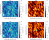 |
Fig. 4 Integrated intensity maps of the two SO transitions over two velocity ranges. Top: J = 77 –66 transition from –7.5 to –2.5 km s−1 (left) and –2.5 to 4.5 km s−1 (right). Bottom: J = 78–67 transition from –7.5 to –2.5 km s−1 (left) and –2.5 to 4.5 km s−1 (right). The peak S/N and rms for each of these maps are listed in Table 2. The black contours are at intervals of σ going from 3σ to peak. |
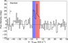 |
Fig. 3 Line profile extracted from within the 3σ extent of the SO stacked integrated intensity with an rms noise of 5.7 mJy and a peak flux of 30.4 mJy resulting in a S/N of 5.3. Highlighted in red and blue are the velocity ranges of emission used in the moment maps of the individual lines in Fig. 4. |
Moment map S/N and rms.
4.2 Confirmation of the SO detection via matched filter analysis
We use a matched filter code1 developed for interferometric data sets to confirm the detection of the two SO lines and to search for emission from the lines undetected in the image plane (Loomis et al. 2017). The detection of weak spectral lines direct from the uv data is optimal as this saves the computational time needed to generate images and eliminates imaging biases. Since the position-velocity pattern of a disk in Keplerian rotation is well characterised, matched filtering can be used to detect weak spectral lines in disks (Loomis et al. 2017). This technique has been shown to increase S/N of the methanol detection in TW Hya by 53% (Walsh et al. 2016b). A filter can either be a strong line detected in the same disk or a model of the anticipated emission. The image cube used as a filter is sampled in the uv plane and these visibilities are cross-correlated with the low S/N visibilities. This is done by sliding the filter though the data channel-by-channel along the velocity axis. If there is a detectable signal, i.e. emission with a similar position and velocity distribution as the filter, the filter response will peak at the source velocity of the emission.
We use the CLEAN image of the CO line (J = 3–2) and the best fit LIME model (see Sect. 5 for details) as filters. The CO image has been scaled down to one quarter of its size and this is motivated by the compact nature of the SO emission (as seen in the channel maps and the integrated intensity: Figs. 1 and 2). Application of the matched filter results in a measure of the response of the filter to the data at a given frequency. The response is scaled to σ with the rms noise normalised to 1.
Figure 5 shows the response of the three detected SO lines to the compact CO and best fit LIME wedge model filters. For the CO filter three of the four lines were detected, the J = 78–67, J = 77–66 and J = 88–77 transitions. They have a peak response of 6.8, 4.2 and 4.0 respectively. There is no detection of the lower energy J = 32–12 transition. We tested different CO filters with different compression factors of 1/2, 1/3 and 1/4. We found that the J = 78–67 transition is picked up in all the filters but the higher excitation lines have an improved response with the more compact filters. The best fit LIME model also detects the same three SO lines. The J = 88–77 filter response is approximately the same as with the compact CO filter but the other two lines responses are quite different.
The peak of the responses are not all at the expected source velocity supporting the theory that we have multiple velocity components of emission including a possible disk wind. The matched filter has confirmed the detection of the two lines detected in the image plane and they are observed at a substantially higher S/N than in the channel maps. It has also facilitated the detection of a line that we do not detect in the imaging. Further, the matched filter line response scales with intensity, so we also now have rudimentary excitation information to motivate our models.
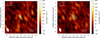 |
Fig. 1 Integrated intensity maps of the two SO transitions integrated over a 11 km s−1 velocity range. Left: J = 77–66 transition with an rms of 22 mJy beam−1 km s−1 and a peak emission of 151 mJy beam−1 km s−1 resulting in a S/N of 6.9. Right: J = 78 –67 transition with an rms of 19 mJy beam−1 km s−1 and a peak emission of 206 mJy beam−1 km s−1 resulting in a S/N of 10.8. The black contours are at intervals of σ from 3σ to peak. |
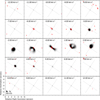 |
Fig. 2 Channel maps of the stacked SO emission (red contours) and the CO J = 3–2 emission with a 3σ clip (grey colour map). The stacked SO emission has with an rms noise of 4.2 mJy beam−1 channel−1 and peak emission of 24.7 mJy beam−1 resulting in a peak S/N of 5.9. The contours are from 3σ to peak in intervals of σ. The stated velocities are with respect to the source velocity. |
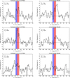 |
Fig. 5 Matched filter responses for the three detected SO transitions. Left: results using a spatially compact (1/4) version of the CO channel maps as a filter. Right: results using the best fit LIME wedge model as a filter (see Sect. 5 for details). Highlighted in red and blue are the velocity ranges of emission we attribute to a disk and a wind component respectively. |
5 Modelling the SO disk emission using LIME
The abundance of SO was estimated by matching the observed emission with simulated emission generated using a HD 100456 physical disk structure (Fig. 6) and LIME version 1.5 (LIne Modelling Engine; Brinch & Hogerheijde 2010). Ray-tracing calculations were done assuming local thermodynamical equilibrium (LTE) and the appropriate distance, inclination and position angle for the source. The molecular data files for sulphur monoxide were taken from the Leiden Atomic and Molecular Database (LAMDA2 ). To check that LTE calculations were a good approximation we calculated the critical density of the transitions. When the number density of gas is greater than the critical density collisional processes dominate. In this regime the level populations are determined by the Boltzmann distribution and LTE is an accurate assumption. The critical density is determined by:
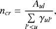
where Aul and γul are the Einstein A and collisional rate coefficients of the transition. The critical density for the SO J = 77–66 transition was determined to be 6 x 106 cm−3 at 100 K using the LAMDA molecular data with the collisional rates from Lique et al. (2006). The other transitions are of a similar order of magnitude.
As the matched filter is a linear process the relative responses for a pair of lines can be used as a proxy for their relative intensities after correcting for the difference in noise levels in each line. These relative intensities were converted to line ratios and this information was used to confine the location of the SO in the disk with respect to the temperature and density conditions. Model line ratios were calculated from line intensities determined using the RADEX3 radiative transfer code assuming an SO column density of 1014 cm−2 motivated by full chemical models. RADEX is a non-LTE 1D radiative transfer code that can be used with the intensity of an observed particular molecular line to estimate the excitation temperature and column density of the gas, assuming an isothermal, homogeneous medium with no significant velocity gradient (van der Tak et al. 2007). The line ratios of the three lines were calculated over a grid of temperatures and densities and the results are shown in Fig. 7. These model line ratios were compared to the observed line ratios from the matched filter responses. Within the velocity range we defined as disk emission, these are 1.5, 1.6 and 1.1 for the J = 78–67/J = 77–66, J = 78–67/J = 87–76 and J = 77–66/J = 87–76 line ratios respectively. A selection of the RADEX results are shown in Table D.1 along with the observed ratios and their associated errors. The regime that best fits our observations is a H2 density from 108 to 1010 cm−3 and a gas temperature between 50 and 100 K. These conditions result in the SO being distributed in a ring from 20 to 100 au in a layer above the mid-plane (see Fig. 6). This is in agreement with previous modelling of sulphur volatiles in disks (e.g. Dutrey et al. 2011) and is in agreement with the compact nature of the SO emission we observe. Placing the SO in a region of lower density and higher temperature resulted in significantly more extended emission than in our observations. We opt to model the near surface of the disk only as we assume that in this region of the disk (<100 au) the optically thick dust emission will block the emission from the molecular gas in the far surface of the disk.
A set of models were run varying the fractional abundance of SO with respect to H2. This was done in order to match the observed peak in the integrated intensity of the disk component for each of the two transitions: 80 mJy beam−1 km s−1 for the J = 77–66 transition and 124 mJy beam−1 km s−1 for the J = 78–67. A model for a full disk was calculated with a fractional abundance of 3.5 × 10⁻⁷ with respect to H2 resulting in a peak intensity for each of the lines of 92 and 109 mJy beam−1 km s−1 respectively. These values match the peak emission of the observations within the ±1σ. The residual maps of the observed integrated intensity minus the model integrated intensity for the two lines are shown in Fig. 8. The residuals show that the observed emission is asymmetric peaking in the north-east region of the disk and that a full disk is not an accurate representation of the data. A second model was run restricting the SO to a specific angular region of the disk. A 45∘ wedge of emission was calculated with the optimal position picked by eye from the residual maps to be from 0∘ to 45∘ from the disk’s major axis. A fractional abundance of 5.0 × 10⁻⁶ with respect to H2 resulted in a peak intensity for each of the lines of 93 mJy beam−1 km s−1 and 96 mJy beam−1 km s−1 respectively. These values match the peak emission of the observations within the ±2σ. This fractional abundance is greater than the “depleted” sulphur fractional abundance observed dark clouds (SO/H2 ≈ 10−8; Ruffle et al. 1999). This suggests that there are energetic processes occurring in HD 100546 releasing a source of refractory sulphur into the gas phase. The fractional abundance of SO derived from the LIME modelling is model dependent as it depends on the gas density of the region of the disk where the SO is located. This model well reproduces the integrated intensity; however, the kinematics trace red-shifted disk emission. The peak in both of the line profiles for the wedge models is 1.7 × the observed line profile peaks and the model emission is over a narrower velocity range. The model line profiles for both the disk and the wedge models are compared with the observed line profiles in Appendix E. Further refinement of the disk emission component requires better data as the emission is the same size scale as the beam.
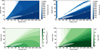 |
Fig. 6 HD 100546 disk physical structure from Kama et al. (2016). Top left and moving clockwise: dust temperature (K), gas temperature (K), UV flux (in units of the interstellar radiation field) and number density (cm−3 ). The two white contours in each of the temperature plots correspond to a temperature of 30 and 50 K. The shaded region highlights the location of the SO motivated by RADEX calculations and used in the LIME modelling. |
 |
Fig. 7 RADEX modelling results of the selected SO line ratios. From left to right are the three ratios: J = 78 –67/J = 77–66, J = 78 –67/J = 87–76 and J = 77–66/J = 87–76. The solid black line is the observed line ratio and the dotted black lines are the error bars. The shaded region highlights the temperature and density conditions chosen for the location of the SO in the LIME modelling. |
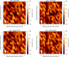 |
Fig. 8 Residual maps from the disk emission integrated intensity and the LIME models for each of the transitions. Top: disk emission minus disk model. Bottom: disk emission minus wedge model. Overlaid are dashed –5, –4 and –3σ contours and solid 3, 4 and 5σ contours. |
6 Discussion
6.1 Location and abundance of the detected SO emission
We detect SO in the protoplanetary disk around HD 100546 for the first time. In the image plane we have a clear detectionof two lines in the integrated intensity maps and we improve the S/N in the channel maps and line profile by stacking. From the morphology of the line profile and the asymmetric distribution of the emission it is likely that we are observing two components of emission: a wedge of disk emission and a blue-shifted component (–5 km s−1). We use a matched filter to better determine the relative intensities of the SO lines in the data set and confirm the detection of three transitions and a non detection of the lowest energy transition. The relative intensities of the three detected lines are used to motivate the location of SO in LIME modelling. The residuals from the observed and modelled integrated intensity maps reveal that the integrated emission is indeed asymmetric peaking north-east of the source position. This is coincident with a “hot-spot” observed in CO emission relating to apossible disk warp (Walsh et al. 2017). The CO J = 3–2 emission from the HD 100546 disk is asymmetric along the minor axis with the emission peaking in the north-east region of the disk. Since this CO emission is optically thick it should be tracing the temperature of the gas and therefore reflects an non-axisymmetric temperature structure. The SO can be modelled as a wedge of emission in this region. The excess blue-shifted (–5 km s−1 with respect to the source velocity) component is spatially inconsistent with the expected location of blue-shifted Keplerian disk emission. We attribute this emission to a disk wind. This hypothesis is summarised in a cartoon in Fig. 9.
We did not detect any of the four SO lines in the complementary HD 97048 Cycle 0 data (see Walsh et al. 2016a) using the imaging methods detailed in Sects. 3 and 4. The stacked emission in the channel maps at a velocity resolution of 1 km s−1 reaches an rms noise of 6 mJy beam−1, and there was no significant response using the matched filter analysis. This supports our hypothesis that SO is tracing a physical mechanism unique to HD 100546. The disks around HD 100546 and HD 97048 have significantly different structures: the gap(s) in the sub-mm dust are further from the star in HD 97048 and there are no protoplanet candidates yet detected in this disk (Quanz et al. 2012; Walsh et al. 2016a; van der Plas et al. 2017). Further detailed modelling is required to determine the chemical origin of the SO emissionin the HD 100546 disk and how the physical and chemical conditions differ from those in the HD 97048 disk.
The only other disk from which SO emission has been imaged is AB Aur (Pacheco-Vázquez et al. 2016). In this transition disk the SO is located further from the star in a ring from approximately 145 to 384 au with a maximum modelled abundance of 2 × 10⁻¹⁰ with respect to H2. The SO, like in HD 100456, is thought to reside in a layer between the surface and the midplane of the disk. The relative abundance of SO observed in AB Aur is a few orders of magnitude less than in HD 100546 and the emission is not necessarily tracing the same process. In AB Aur, SO is proposed as a chemical tracer of the early stages of planet formation as the abundance of SO appears to decrease towards the disk’s dust trap, a local pressure maximum thought to be the site of future plant formation (e.g. van der Marel et al. 2013).
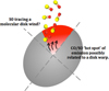 |
Fig. 9 Cartoon of HD 100546 showing the wedge region of disk emission and the disk wind traced in SO. |
6.2 Sulphur chemistry in the HD 100546 disk
Sulphur chemistry, particularly the evolution of S-bearing molecules on grain surfaces, is not fully understood as current models fail to reproduce observed abundances (e.g. Guilloteau et al. 2016). If we are observing a wedge or partial ring of SO, the inner edge of the emission coincides with the inner edge of the sub-millimetre dust ring at approximately 20 au. Since HD 100546 is a transition disk the midplane material is exposed to far-UV photons from the central star. This will cause the desorption of molecules from icy grain mantles. H2 O ice has been observed in this disk (Honda et al. 2016) and H2 S ice is a primary component of cometary ices (Bockelée-Morvan et al. 2000). The photodissociation of these molecules originating from cosmic rays or UV photons, depending on the height of the gas in the disk, would create the reactants needed to form SO;
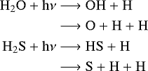
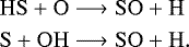
The activation energy, EA, of the two SO formation reactions is zero (KIDA: KInetic Database for Astrochemistry4). There are a few possible reactions for the destruction of SO to form SO2 (Millar & Herbst 1990);


In AB Aur the abundance of SO decreases with increasing density towards the disk’s dust trap. This is attributed to the increase in conversion of SO to SO2 via radiativeassociation with atomic oxygen and then freeze out of SO2 onto dust grains (Pacheco-Vázquez et al. 2016). In HD 100546, the density and temperature of the disk may have been perturbed creating the conditions for the localised formation of the observed asymmetric SO. However, chemical modelling of warped disks and associated temperature perturbations are required to confirm this hypothesis.
From observations of cometary volatiles, and for the particular case of 67P, the total abundance of sulphur-bearing species detected is consistent with the solar abundance of sulphur (Calmonte et al. 2016). This means that if our solar system is typical then the observed depletion of sulphur in circumstellar regions may be an observational effect as we have not been able to detect the various forms of sulphur. The form of the sulphur, whether it resides in refractory or volatile form in planet-forming disks is still an open question. For the SO we detect in HD 100546 it is unclear as to its origin, e.g., if it is a result of the volatile reactions described above or whether it has been released from refractory materials due to a shock as suggested by the abundance we determine. Further observations may make this clearer.
6.3 What is the SO tracing?
The influence of the massive companion at approximately 10 au in the disk may cause the disk velocity structure to depart from simple Keplerian rotation in the inner region. The protoplanet embedded in the disk at 50 au may also have an effect (Quillen 2006). If the disk is warped, the line of sight inclination will vary radially changing the velocity structure. Previous observations with APEX show that the 12CO emission from the HD 100546 protoplanetary disk is asymmetric (Panić et al. 2010) suggesting that one side of the outer disk is colder by 10–20 K than the other or that there is a shadow on the outer disk caused by a warped geometry of the inner disk. Shadows resulting from disk warps and their effect on gas kinematics have been observed in a few other sources e.g. HD 142527 (Casassus et al. 2015). There is evidence for a possible warp in the inner 100 au of the HD 100546 disk from a detailed study of the CO J = 3–2 kinematics (Walsh et al. 2017). The spatial resolution of the HD 100546 Cycle 0 observations is limited to approximately 100 au along the minor axis of the disk so it is unclear what is causing the non-Keplerian motions. Since previous observations point towards this star hosting at least one massive companion, a warped disk is a favoured hypothesis. A warp would directly expose the north-east side of the disk to heating by the central star, creating locally the conditions for the formation of SO and the launching of a disk wind. The non-Keplerian motions in the inner 100 au of this disk could explain the discrepancy in the kinematics of the best fit model for the SO and the observations.
Disk dispersal is predicted to occur on a timescale up to 10 times shorter than observed disk lifetimes (Alexander et al. 2014). This process limits the time available for giant plant formation, decreases the gas to dust ratio in the disk, and the mass loss will have an effect on the chemical content of the disk. In planet-forming Class II disks, jets/outflows are not the main driver of disk dispersal. Instead the removal of angular momentum from the disk material can be achieved by slower disk winds (<30 km s−1). Photoevaporative disk winds are thought to be the primary disk dispersal mechanism (Alexander et al. 2014). MHD disk winds also drive disk dispersal but are less well understood (Ercolano & Pascucci 2017). Evidence of photoevaporative disk winds has been detected from a number of sources in the form of blue-shifted (up to 10 km s−1) line profiles of forbidden line emission in the optical (e.g. Pascucci et al. 2011; Ercolano & Owen 2016). In addition to this, ALMA observations show a spatially resolved molecular disk wind originating from the HD 163296 disk (Klaassen et al. 2013), and a molecular protostellar outflow from TMC1A launched by a disk wind originating from a Keplerian disk (Bjerkeli et al. 2016). We checked for any large scale or high velocity ( >10 km s−1) CO or SO emission from HD 100546 but none was detected. Gas launched from the HD 100546 disk surface with a velocity of a few km s−1 would have a blue shift along the line of sight to the observer and could account for the blue-shifted emission that we observe. The mechanism for launching this material and why it is traced in the SO emission is unclear. The lack of observed excess blue-shifted CO emission is due to the SO originating from a layer in the disk that is higher than the emitting layer of the CO J = 3–2 (Eu = 33.19 K) gas. To see this effect in CO will require observations of higher J lines which will be tracing the warmer gas in the atmosphere. We surmise that the red-shifted counterpart of the disk wind, launching from the far side of the disk, is obscured by the optically thick dust disk. Determination of the chemical origin of the SO will help to shed light on whether the wind is MHD driven (ion-molecule chemistry) or photoevaporative (photon-dominated chemistry) in nature.
An alternative explanation for the SO emission is that it is the result of an accretion shock due to a circumplanetary disk. The position angle of the SO emission coincides with the observed infrared point source in the disk at approximately 50 au that has been attributed to a protoplanet (Quanz et al. 2013; Currie et al. 2015).
7 Conclusions
We have shown that SO is detectable in protoplanetary disks with ALMAuncovering a sulphur reservoir in the HD 100546 protoplanetary disk. In addition, we have shown that SO may be a tracer of a molecular disk wind. New data with better spatial and spectral resolution are required to truly disentangle the disk and wind components of the emission. This will allow for an accurate determination of the spatial distribution of the disk emission and the launch region of the wind. Observations of sulphur-bearing species in this disk and others will help to constrain the fraction of the cosmic abundance of sulphur partitioned into refractory and volatile material. Transition disks are important targets as their cavities may expose the hidden sulphur.
Acknowledgements
The authors thank Dr Pamela Klaassen for useful discussions on this work. This paper makes use of the following ALMA data: ADS/JAO.ALMA#2011.0.00863.S ALMA is a partnership of ESO (representing its member states), NSF (USA) and NINS (Japan), together with NRC (Canada), NSC and ASIAA (Taiwan), and KASI (Republic of Korea), in cooperation with the Republic of Chile. The Joint ALMA Observatoryis operated by ESO, AUI/NRAO and NAOJ. A.B. acknowledges the studentship funded by the Science and Technology Facilities Council of the United Kingdom (STFC). C.W. acknowledges financial support from the Netherlands Organisation for Scientific Research (NWO, grant 639.041.335) and start-up funds from the University of Leeds, UK. M.K. gratefully acknowledges funding from the European Union’s Horizon 2020 research and innovation programme under the Marie Sklodowska-Curie grant agreement No. 753799. R.A.L. gratefully acknowledges funding from the NRAO Student Observing Support program. A.J. is supported by the DISCSIM project, grant agreement 341137 funded by the European Research Council under ERC-2013-ADG.
Appendix A Individual line profiles
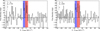 |
Fig. A.1 Line profiles of the individual J = 77–66 (left) and J = 78–67 (right) transitions extracted from within the 3σ extent of their respective intensity maps. Both line profiles reach a S/N of 3 with rms noise of 10.8 and 8.7 mJy, respectively. Highlighted in red and blue are the velocity ranges of emission used in the moment maps in Fig. 4. |
Appendix B Stacked SO and CO J = 3–2 line profiles
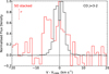 |
Fig. B.1 SO stacked (red) line profile and CO J = 3–2 (black) line profile extracted from within the 3σ extent of their respective integrated intensity maps. The SO stacked line profile reaches a S/N of 5 and the CO J = 3–2 reaches a S/N of 375. Note that the rms for the CO J = 3–2 is not visible on this scale (81 mJy). |
Appendix C Stacked moment maps
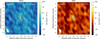 |
Fig. C.1 Integrated intensity maps of the stacked SO emission over two velocity ranges: –7.5 to –2.5 km s−1 (left) with a S/N of 7 and –2.5 to 4.5 km s−1 (right) with a S/N of 9. The rms noise reached in these maps is 11 and 14 mJy beam−1 km s−1 and the peakemission is 80 and 123 mJy beam−1 km s−1, respectively. The black contours are at intervals of σ from 3σ to peak. |
Appendix D RADEX line ratios
Model and observed line ratios for the detected SO transitions.
Appendix E Individual line profiles and LIME disk model line profiles
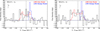 |
Fig. E.1 Line profiles of the individual J = 77 − 66 (left) and J = 78 − 67 (right) transitions with the LIME model line profiles plotted on the top: disk model (red) and wedge model (blue). |
References
- Acke, B., & van den Ancker, M. E. 2006, A&A 449, 267 [NASA ADS] [CrossRef] [EDP Sciences] [Google Scholar]
- Alexander, R., Pascucci, I., Andrews, S., Armitage, P., & Cieza, L. 2014, Protostars and Planets VI, (Tucson, AZ: Univ. Arizona Press), ed. H. Beuther et al., 475 [Google Scholar]
- Avenhaus, H., Quanz, S. P., Meyer, M. R., et al. 2014, ApJ 790, 56 [NASA ADS] [CrossRef] [Google Scholar]
- Benisty, M., Tatulli, E., Ménard, F., & Swain, M. R. 2010, A&A 511, A75 [NASA ADS] [CrossRef] [EDP Sciences] [Google Scholar]
- Benisty, M., Stolker, T., Pohl, A., et al. 2017, A&A 597, A42 [NASA ADS] [CrossRef] [EDP Sciences] [Google Scholar]
- Bjerkeli, P., van der Wiel, M. H. D., Harsono, D., Ramsey, J. P., & Jørgensen, J. K. 2016, Nature 540, 406 [NASA ADS] [CrossRef] [Google Scholar]
- Bockelée-Morvan, D., Lis, D. C., Wink, J. E., et al. 2000, A&A 353, 1101 [Google Scholar]
- Bouwman, J., de Koter, A., Dominik, C., & Waters, L. B. F. M. 2003, A&A 401, 577 [NASA ADS] [CrossRef] [EDP Sciences] [Google Scholar]
- Brinch, C., & Hogerheijde, M. R. 2010, A&A 523, A25 [NASA ADS] [CrossRef] [EDP Sciences] [Google Scholar]
- Brittain, S. D., Najita, J. R., & Carr, J. S. 2009, ApJ 702, 85 [NASA ADS] [CrossRef] [Google Scholar]
- Brittain, S. D., Carr, J. S., Najita, J. R., Quanz, S. P., & Meyer, M. R. 2014, ApJ 791, 136 [NASA ADS] [CrossRef] [Google Scholar]
- Bruderer, S., van Dishoeck, E. F., Doty, S. D., & Herczeg, G. J. 2012, A&A 541, A91 [NASA ADS] [CrossRef] [EDP Sciences] [Google Scholar]
- Calmonte, U., Altwegg, K., Balsiger, H., et al. 2016, MNRAS 462, S253 [CrossRef] [Google Scholar]
- Carmona, A., van der Plas, G., van den Ancker, M. E., et al. 2011, A&A 533, A39 [NASA ADS] [CrossRef] [EDP Sciences] [Google Scholar]
- Casassus, S., Marino, S., Perez, S., et al. 2015, ApJ 811, 92 [NASA ADS] [CrossRef] [Google Scholar]
- Cleeves, L. I., Bergin, E. A., Bethell, T. J., et al. 2011, ApJ 743, L2 [NASA ADS] [CrossRef] [Google Scholar]
- Currie, T., Muto, T., Kudo, T., et al. 2014, ApJ 796, L30 [NASA ADS] [CrossRef] [Google Scholar]
- Currie, T., Cloutier, R., Brittain, S., et al. 2015, ApJ 814, L27 [NASA ADS] [CrossRef] [Google Scholar]
- Dutrey, A., Guilloteau, S., & Guelin, M. 1997, A&A 317, L55 [NASA ADS] [Google Scholar]
- Dutrey, A., Wakelam, V., Boehler, Y., et al. 2011, A&A 535, A104 [NASA ADS] [CrossRef] [EDP Sciences] [Google Scholar]
- Dutrey, A., Semenov, D., Chapillon, E., et al. 2014, Protostars and Planets VI, (Tucson, AZ: Univ. Arizona Press), ed. H. Beuther et al., 317 [Google Scholar]
- Ercolano, B., & Owen, J. E. 2016, MNRAS 460, 3472 [NASA ADS] [CrossRef] [Google Scholar]
- Ercolano, B., & Pascucci, I. 2017, R. Soc. Open Sci. 4, 170114 [Google Scholar]
- Fedele, D., Bruderer, S., van Dishoeck, E. F., et al. 2013, A&A 559, A77 [NASA ADS] [CrossRef] [EDP Sciences] [Google Scholar]
- Fuente, A., Cernicharo, J., Agúndez, M., et al. 2010, A&A 524, A19 [NASA ADS] [CrossRef] [EDP Sciences] [Google Scholar]
- Gaia Collaboration (Brown, A. G. A., et al.) 2016a, A&A 595, A2 [NASA ADS] [CrossRef] [EDP Sciences] [Google Scholar]
- Gaia Collaboration (Prusti, T., et al.) 2016b, A&A 595, A1 [NASA ADS] [CrossRef] [EDP Sciences] [Google Scholar]
- Garufi, A., Quanz, S. P., Schmid, H. M., et al. 2016, A&A 588, A8 [NASA ADS] [CrossRef] [EDP Sciences] [Google Scholar]
- Goto, M., van der Plas, G., van den Ancker, M., et al. 2012, A&A 539, A81 [NASA ADS] [CrossRef] [EDP Sciences] [Google Scholar]
- Guilloteau, S., Di Folco, E., Dutrey, A., et al. 2013, A&A 549, A92 [NASA ADS] [CrossRef] [EDP Sciences] [Google Scholar]
- Guilloteau, S., Reboussin, L., Dutrey, A., et al. 2016, A&A 592, A124 [NASA ADS] [CrossRef] [EDP Sciences] [Google Scholar]
- Hein Bertelsen, R. P., Kamp, I., Goto, M., et al. 2014, A&A 561, A102 [NASA ADS] [CrossRef] [EDP Sciences] [Google Scholar]
- Henning, T., & Semenov, D. 2013, Chem. Rev. 113, 9016 [Google Scholar]
- Honda, M., Kudo, T., Takatsuki, S., et al. 2016, ApJ 821, 2 [NASA ADS] [CrossRef] [Google Scholar]
- Kama, M., Bruderer, S., van Dishoeck, E. F., et al. 2016, A&A 592, A83 [NASA ADS] [CrossRef] [EDP Sciences] [Google Scholar]
- Keller, L. P., Hony, S., Bradley, J. P., et al. 2002, Nature 417, 148 [NASA ADS] [CrossRef] [PubMed] [Google Scholar]
- Klaassen, P. D., Juhasz, A., Mathews, G. S., et al. 2013, A&A 555, A73 [NASA ADS] [CrossRef] [EDP Sciences] [Google Scholar]
- Lique, F., Dubernet, M.-L., Spielfiedel, A., & Feautrier, N. 2006, A&A 450, 399 [NASA ADS] [CrossRef] [EDP Sciences] [Google Scholar]
- Liskowsky, J. P., Brittain, S. D., Najita, J. R., et al. 2012, ApJ 760, 153 [NASA ADS] [CrossRef] [Google Scholar]
- Loomis, R. A., Öberg, K. I., Andrews, S. M., et al. 2017, A&A, submitted [Google Scholar]
- Martín-Doménech, R., Jiménez-Serra, I., Muñoz Caro, G. M., et al. 2016, A&A, 585, A112 [NASA ADS] [CrossRef] [EDP Sciences] [Google Scholar]
- Meeus, G., Salyk, C., Bruderer, S., et al. 2013, A&A 559, A84 [NASA ADS] [CrossRef] [EDP Sciences] [Google Scholar]
- Millar, T. J., & Herbst, E. 1990, A&A 231, 466 [NASA ADS] [Google Scholar]
- Mulders, G. D., Paardekooper, S.-J., Panić, O., et al. 2013, A&A 557, A68 [NASA ADS] [CrossRef] [EDP Sciences] [Google Scholar]
- Müller, H. S. P., Thorwirth, S., Roth, D. A., & Winnewisser, G. 2001, A&A 370, L49 [NASA ADS] [CrossRef] [EDP Sciences] [Google Scholar]
- Ohashi, N., Saigo, K., Aso, Y., et al. 2014, ApJ 796, 131 [NASA ADS] [CrossRef] [Google Scholar]
- Pacheco-Vázquez, S., Fuente, A., Agúndez, M., et al. 2015, A&A 578, A81 [NASA ADS] [CrossRef] [EDP Sciences] [Google Scholar]
- Pacheco-Vázquez, S., Fuente, A., Baruteau, C., et al. 2016, A&A 589, A60 [NASA ADS] [CrossRef] [EDP Sciences] [Google Scholar]
- Panić, O., van Dishoeck, E. F., Hogerheijde, M. R., et al. 2010, A&A, 519, A110 [NASA ADS] [CrossRef] [EDP Sciences] [Google Scholar]
- Pascucci, I., Sterzik, M., Alexander, R. D., et al. 2011, ApJ 736, 13 [NASA ADS] [CrossRef] [Google Scholar]
- Pineda, J. E., Quanz, S. P., Meru, F., et al. 2014, ApJ 788, L34 [NASA ADS] [CrossRef] [Google Scholar]
- Pinilla, P., Birnstiel, T., & Walsh, C. 2015, A&A 580, A105 [NASA ADS] [CrossRef] [EDP Sciences] [Google Scholar]
- Podio, L., Codella, C., Gueth, F., et al. 2015, A&A 581, A85 [NASA ADS] [CrossRef] [EDP Sciences] [Google Scholar]
- Quanz, S. P., Birkmann, S. M., Apai, D., Wolf, S., & Henning, T. 2012, A&A 538, A92 [NASA ADS] [CrossRef] [EDP Sciences] [Google Scholar]
- Quanz, S. P., Amara, A., Meyer, M. R., et al. 2013, ApJ 766, L1 [NASA ADS] [CrossRef] [Google Scholar]
- Quanz, S. P., Amara, A., Meyer, M. R., et al. 2015, ApJ 807, 64 [NASA ADS] [CrossRef] [Google Scholar]
- Quillen, A. C. 2006, ApJ 640, 1078 [NASA ADS] [CrossRef] [Google Scholar]
- Reggiani, M., Quanz, S. P., Meyer, M. R., et al. 2014, ApJ 792, L23 [NASA ADS] [CrossRef] [Google Scholar]
- Ruffle, D. P., Hartquist, T. W., Caselli, P., & Williams, D. A. 1999, MNRAS 306, 691 [NASA ADS] [CrossRef] [Google Scholar]
- Sakai, N., Oya, Y., López-Sepulcre, A., et al. 2016, ApJ 820, L34 [NASA ADS] [CrossRef] [Google Scholar]
- Sallum, S., Follette, K. B., Eisner, J. A., et al. 2015, Nature 527, 342 [NASA ADS] [CrossRef] [Google Scholar]
- Schöier, F. L., van der Tak, F. F. S., van Dishoeck, E. F., & Black, J. H. 2005, A&A 432, 369 [NASA ADS] [CrossRef] [EDP Sciences] [Google Scholar]
- Strom, K. M., Strom, S. E., Edwards, S., Cabrit, S., & Skrutskie, M. F. 1989, AJ 97, 1451 [NASA ADS] [CrossRef] [Google Scholar]
- Sturm, B., Bouwman, J., Henning, T., et al. 2010, A&A 518, L129 [NASA ADS] [CrossRef] [EDP Sciences] [Google Scholar]
- Tafalla, M., Santiago-García, J., Hacar, A., & Bachiller, R. 2010, A&A, 522, A91 [NASA ADS] [CrossRef] [EDP Sciences] [Google Scholar]
- Tatulli, E., Benisty, M., Ménard, F., et al. 2011, A&A 531, A1 [NASA ADS] [CrossRef] [EDP Sciences] [Google Scholar]
- Thi, W.-F., Ménard, F., Meeus, G., et al. 2011, A&A 530, L2 [NASA ADS] [CrossRef] [EDP Sciences] [Google Scholar]
- Tieftrunk, A., Pineau des Forets, G., Schilke, P., & Walmsley, C. M. 1994, A&A 289, 579 [Google Scholar]
- van den Ancker, M. E., de Winter, D., & Tjin A Djie, H. R. E. 1998, A&A 330, 145 [NASA ADS] [Google Scholar]
- van der Marel, N., van Dishoeck, E. F., Bruderer, S., et al. 2013, Science 340, 1199 [NASA ADS] [CrossRef] [PubMed] [Google Scholar]
- van der Plas, G., van den Ancker, M. E., Acke, B., et al. 2009, A&A 500, 1137 [NASA ADS] [CrossRef] [EDP Sciences] [Google Scholar]
- van der Plas, G., Wright, C. M., Ménard, F., et al. 2017, A&A 597, A32 [NASA ADS] [CrossRef] [EDP Sciences] [Google Scholar]
- van der Tak, F. F. S., Black, J. H., Schöier, F. L., Jansen, D. J., & van Dishoeck E. F. 2007, A&A 468, 627 [NASA ADS] [CrossRef] [EDP Sciences] [Google Scholar]
- Walsh, C., Juhász, A., Pinilla, P., et al. 2014, ApJ 791, L6 [NASA ADS] [CrossRef] [Google Scholar]
- Walsh, C., Juhász, A., Meeus, G., et al. 2016a, ApJ 831, 200 [NASA ADS] [CrossRef] [Google Scholar]
- Walsh, C., Loomis, R. A., Öberg, K. I., et al. 2016b, ApJ 823, L10 [NASA ADS] [CrossRef] [Google Scholar]
- Walsh, C., Daley, C., Facchini, S., & Juhász, A. 2017, A&A 607, A114 [NASA ADS] [CrossRef] [EDP Sciences] [Google Scholar]
vis_sample is publicly available at: https://github.com/AstroChem/vis_sample
All Tables
ALMA band 7 observational parameters and sulphur monoxide transitions for HD 100546.
All Figures
|
Fig. 4 Integrated intensity maps of the two SO transitions over two velocity ranges. Top: J = 77 –66 transition from –7.5 to –2.5 km s−1 (left) and –2.5 to 4.5 km s−1 (right). Bottom: J = 78–67 transition from –7.5 to –2.5 km s−1 (left) and –2.5 to 4.5 km s−1 (right). The peak S/N and rms for each of these maps are listed in Table 2. The black contours are at intervals of σ going from 3σ to peak. |
| In the text | |
|
Fig. 3 Line profile extracted from within the 3σ extent of the SO stacked integrated intensity with an rms noise of 5.7 mJy and a peak flux of 30.4 mJy resulting in a S/N of 5.3. Highlighted in red and blue are the velocity ranges of emission used in the moment maps of the individual lines in Fig. 4. |
| In the text | |
|
Fig. 1 Integrated intensity maps of the two SO transitions integrated over a 11 km s−1 velocity range. Left: J = 77–66 transition with an rms of 22 mJy beam−1 km s−1 and a peak emission of 151 mJy beam−1 km s−1 resulting in a S/N of 6.9. Right: J = 78 –67 transition with an rms of 19 mJy beam−1 km s−1 and a peak emission of 206 mJy beam−1 km s−1 resulting in a S/N of 10.8. The black contours are at intervals of σ from 3σ to peak. |
| In the text | |
|
Fig. 2 Channel maps of the stacked SO emission (red contours) and the CO J = 3–2 emission with a 3σ clip (grey colour map). The stacked SO emission has with an rms noise of 4.2 mJy beam−1 channel−1 and peak emission of 24.7 mJy beam−1 resulting in a peak S/N of 5.9. The contours are from 3σ to peak in intervals of σ. The stated velocities are with respect to the source velocity. |
| In the text | |
|
Fig. 5 Matched filter responses for the three detected SO transitions. Left: results using a spatially compact (1/4) version of the CO channel maps as a filter. Right: results using the best fit LIME wedge model as a filter (see Sect. 5 for details). Highlighted in red and blue are the velocity ranges of emission we attribute to a disk and a wind component respectively. |
| In the text | |
|
Fig. 6 HD 100546 disk physical structure from Kama et al. (2016). Top left and moving clockwise: dust temperature (K), gas temperature (K), UV flux (in units of the interstellar radiation field) and number density (cm−3 ). The two white contours in each of the temperature plots correspond to a temperature of 30 and 50 K. The shaded region highlights the location of the SO motivated by RADEX calculations and used in the LIME modelling. |
| In the text | |
|
Fig. 7 RADEX modelling results of the selected SO line ratios. From left to right are the three ratios: J = 78 –67/J = 77–66, J = 78 –67/J = 87–76 and J = 77–66/J = 87–76. The solid black line is the observed line ratio and the dotted black lines are the error bars. The shaded region highlights the temperature and density conditions chosen for the location of the SO in the LIME modelling. |
| In the text | |
|
Fig. 8 Residual maps from the disk emission integrated intensity and the LIME models for each of the transitions. Top: disk emission minus disk model. Bottom: disk emission minus wedge model. Overlaid are dashed –5, –4 and –3σ contours and solid 3, 4 and 5σ contours. |
| In the text | |
|
Fig. 9 Cartoon of HD 100546 showing the wedge region of disk emission and the disk wind traced in SO. |
| In the text | |
|
Fig. A.1 Line profiles of the individual J = 77–66 (left) and J = 78–67 (right) transitions extracted from within the 3σ extent of their respective intensity maps. Both line profiles reach a S/N of 3 with rms noise of 10.8 and 8.7 mJy, respectively. Highlighted in red and blue are the velocity ranges of emission used in the moment maps in Fig. 4. |
| In the text | |
|
Fig. B.1 SO stacked (red) line profile and CO J = 3–2 (black) line profile extracted from within the 3σ extent of their respective integrated intensity maps. The SO stacked line profile reaches a S/N of 5 and the CO J = 3–2 reaches a S/N of 375. Note that the rms for the CO J = 3–2 is not visible on this scale (81 mJy). |
| In the text | |
|
Fig. C.1 Integrated intensity maps of the stacked SO emission over two velocity ranges: –7.5 to –2.5 km s−1 (left) with a S/N of 7 and –2.5 to 4.5 km s−1 (right) with a S/N of 9. The rms noise reached in these maps is 11 and 14 mJy beam−1 km s−1 and the peakemission is 80 and 123 mJy beam−1 km s−1, respectively. The black contours are at intervals of σ from 3σ to peak. |
| In the text | |
|
Fig. E.1 Line profiles of the individual J = 77 − 66 (left) and J = 78 − 67 (right) transitions with the LIME model line profiles plotted on the top: disk model (red) and wedge model (blue). |
| In the text | |
Current usage metrics show cumulative count of Article Views (full-text article views including HTML views, PDF and ePub downloads, according to the available data) and Abstracts Views on Vision4Press platform.
Data correspond to usage on the plateform after 2015. The current usage metrics is available 48-96 hours after online publication and is updated daily on week days.
Initial download of the metrics may take a while.