| Issue |
A&A
Volume 611, March 2018
|
|
|---|---|---|
| Article Number | A24 | |
| Number of page(s) | 15 | |
| Section | Interstellar and circumstellar matter | |
| DOI | https://doi.org/10.1051/0004-6361/201731071 | |
| Published online | 20 March 2018 | |
The FRIGG project: From intermediate galactic scales to self-gravitating cores
1
Université Paris Diderot, AIM, Sorbonne Paris Cité, CEA, CNRS,
91191
Gif-sur-Yvette, France
e-mail: This email address is being protected from spambots. You need JavaScript enabled to view it.
2
LERMA (UMR CNRS 8112), Ecole Normale Supérieure,
75231
Paris Cedex, France
Received:
29
April
2017
Accepted:
20
September
2017
Abstract
Context. Understanding the detailed structure of the interstellar gas is essential for our knowledge of the star formation process.
Aim. The small-scale structure of the interstellar medium (ISM) is a direct consequence of the galactic scales and making the link between the two is essential.
Methods. We perform adaptive mesh simulations that aim to bridge the gap between the intermediate galactic scales and the self-gravitating prestellar cores. For this purpose we use stratified supernova regulated ISM magneto-hydrodynamical simulations at the kpc scale to set up the initial conditions. We then zoom, performing a series of concentric uniform refinement and then refining on the Jeans length for the last levels. This allows us to reach a spatial resolution of a few 10−3 pc. The cores are identified using a clump finder and various criteria based on virial analysis. Their most relevant properties are computed and, due to the large number of objects formed in the simulations, reliable statistics are obtained.
Results. The cores’ properties show encouraging agreements with observations. The mass spectrum presents a clear powerlaw at high masses with an exponent close to ≃−1.3 and a peak at about 1–2 M⊙. The velocity dispersion and the angular momentum distributions are respectively a few times the local sound speed and a few 10−2 pc km s−1. We also find that the distribution of thermally supercritical cores present a range of magnetic mass-to-flux over critical mass-to-flux ratios, typically between ≃0.3 and 3 indicating that they are significantly magnetized. Investigating the time and spatial dependence of these statistical properties, we conclude that they are not significantly affected by the zooming procedure and that they do not present very large fluctuations. The most severe issue appears to be the dependence on the numerical resolution of the core mass function (CMF). While the core definition process may possibly introduce some biases, the peak tends to shift to smaller values when the resolution improves.
Conclusions. Our simulations, which use self-consistently generated initial conditions at the kpc scale, produce a large number of prestellar cores from which reliable statistics can be inferred. Preliminary comparisons with observations show encouraging agreements. In particular the inferred CMFs resemble the ones inferred from recent observations. We stress, however, a possible issue with the peak position shifting with numerical resolution.
Key words: ISM: clouds / ISM: magnetic fields / ISM: structure / stars: formation / turbulence
© ESO 2018
1 Introduction
One of the aspects limiting our understanding of the star formation process is its multi-scale nature. While the conditions that lead to the formation of molecular clouds, where star birth takes place, are induced by the large and intermediate galactic scales, the ultimate mass reservoir of stars, the prestellar cores, are only a few 10−2 pc wide (e.g., Ward-Thompson et al. 2007; Offner et al. 2014). This implies that ideally one would need to obtain a continuous description of spatial scales going from at least a few hundreds to a few hundredths of pc.
Various studies have investigated the core formation in simulations but fewer have attempted to provide statistics of the core properties. Typically, a box of a few pc across is specified with a prescribed mean density and velocity dispersion and the turbulence is either driven or free to decay. The simulations are either hydrodynamical or magneto-hydrodynamical (MHD; Klessen et al. 1998, 2005; Klessen & Burkert 2001; Vázquez-Semadeni et al. 2005; Offner et al. 2008; Dib et al. 2010; Gong & Ostriker 2011, 2015) and some model the ambipolar diffusion (van Loo et al. 2008; Kudoh & Basu 2008, 2011; Chen & Ostriker 2014). While this kind of approach offers a natural framework to study the core formation in detail, two difficulties are encountered. First of all, the core properties, such as their mass distribution, directly depend on the simulation parameters (e.g., Klessen & Burkert 2000; Gong & Ostriker 2015), for example the mean Jeans mass, thus it is necessary to perform an ensemble of simulations, and for the purpose of comparing with observations, to convolve the core distribution by the distribution of large-scale initial conditions. Second, the number of cores formed is often restricted to a small number limiting the inferred statistics.
In an attempt to circumvent these two difficulties but also to bridge the gap between the intermediate galactic scales, that is to say, the scales of a few hundreds of pc, and the scales of the self-gravitating prestellar cores, that is, on the order of 0.1 pc, we perform zooming simulations starting from self-consistently generated initial conditions. The benefit of this approach is that there is no need to specify the initial conditions of the dense molecular phase. A distribution of molecular clouds is naturally produced from the diffuse atomic gas. The initial setup is very similar to the studies described in Hennebelle & Iffrig (2014) and Iffrig & Hennebelle (2017; see also Korpi et al. 1999; Slyz et al. 2005; de Avillez & Breitschwerdt 2005; Joung & Mac Low 2006; Hill et al. 2012; Kim et al. 2011, 2013; Gent et al. 2013; Gatto et al. 2015). These studies consider a kpc stratified galactic box. The interstellar medium (ISM) is self-regulated by the star formation process and the associated supernova explosions, which inject energy and momentum and sustain the turbulence. The finest spatial resolution obtained in the simulations is a few 10−3 pc and allows us to describe the formation of cores with masses larger than a few 0.1 M⊙, while the region hundreds of pc in size, where full zooming is applied, leads to a large number of cores from which reliable statistics can be obtained.
We note that other zooming simulations have been performed in the context of the star formation studies, such as for example the ones by Offner et al. (2008) and Padoan et al. (2014), which started from molecular cloud scales and zoom up to scales of a few tens of AU. At the kpc scale, the deepest zoom simulations have been performed by Butler et al. (2015), where the spatial resolution goes up to 0.1 pc (see also Seifried et al. 2017). To our knowledge the simulation presented here is the first to make the link between scales of a few hundred pc and those of a few thousand AU.
The plan of the paper is as follows. In the second section, we describe the numerical setup, the physics included in the simulations, as well as the zooming procedure that we employed. The third section explains the algorithm used to identify the cores in 3D space and gives the definition of the computed quantities. In the fourth section we present the structure and the core statistics obtained for various definition and criteria. In the fifth section, we look at various subregions and a subset of cores to explore their dependence to environments. In sixth section, we investigate the time dependence of the statistics with the aim of assessing the robustness of the results. We also compare the results obtained with three different spatial resolutions. Finally Sect. 7 concludes the paper.
2 General setup
2.1 Code and processes
To perform our simulations, we employ the code RAMSES (Teyssier 2002; Fromang et al. 2006), which is an adaptive mesh refinement code working in Cartesian geometry and using finite volume methods and Godunov solvers to solve the MHD equations. Ramses uses a constraint transport scheme for the magnetic field, which preserves div B to machine precision.
As described below, we make extensive use of the AMR scheme and starting from level 9 we introduce another 8 to 10 AMR levels, therefore reaching levels 17–19.
The simulations include various physical processes known to be important in the ISM. The ideal MHD equations with self-gravity are solved and take into account the cooling and heating processes relevant to the ISM, which include UV heating and a cooling function with the same low-temperature part as in Audit & Hennebelle (2005) and the high-temperature part based on Sutherland & Dopita (1993), resulting in a function similar to the one used in Joung & Mac Low (2006).
An analytical gravity profile accounting for the distribution of stars and dark matter is added. The corresponding gravitational potential is given by (Kuijken & Gilmore 1989):
 (1)
(1)
with a1 = 1.42 × 10⁻³ kpc Myr−2, a2 = 5.49 × 10⁻⁴ Myr−2 and z0 = 180 pc, as used by Joung & Mac Low (2006). The gravitational potential Φ has thus two terms, the one due to stars and dark matter ϕext, and the one due to the gas itself ϕ, hence Φ = ϕ + ϕext.
2.2 Initial conditions
We initialize our simulations with a stratified disc: we use a Gaussian density profile:
![Mathematical equation: $ n(z) = n_0 \exp \left[ - \frac{1}{2} \left( \frac{z}{z_0} \right)^2 \right], $](/articles/aa/full_html/2018/03/aa31071-17/aa31071-17-eq2.png) (2)
(2)
where n0 = 1.5 cm-3 and z0 = 150 pc. This leads to a total column density, Σ, through the disc that is equal to  where ρ0 = mpn0 and mp = 2.3 × 10⁻²⁴ g is the mean mass per particle, which corresponds to a mixture of hydrogen and about 10% of helium as in the ISM. We obtain Σ = 4 × 10⁻³ g cm−2 = 19.1M⊙ pc−2.
The temperature is set to a usual warm neutral medium (WNM) temperature, around 8000 K. In order to prevent this disc from collapsing, an initial turbulent velocity field is generated with a dispersion of 5 km s−1 and a Kolmogorov (Kolmogorov 1941) power spectrum with random phase. The initial horizontal magnetic field is given by
![Mathematical equation: $ B_x(z) = B_0 \exp \left[ - \frac{1}{2} \left( \frac{z}{z_0} \right)^2 \right], $](/articles/aa/full_html/2018/03/aa31071-17/aa31071-17-eq4.png) (3)
(3)
with B0 ≃ 3 μG.
2.3 Strategy for zooming simulations
The primary goal of the present study is to link the intermediate scales of galaxies, that is to say the scales on the order of 100 pc−1 kpc, with the ones of the dense cores, thought to be the mass reservoir of stars. Dense cores have typical sizes on the order of, and possibly slightly below, 0.1 pc (Ward-Thompson et al. 2007; Könyves et al. 2015). To properly describe this scale, it is necessary to use, at the very least, 10 cells across the cores and thus to reach a spatial resolution of at least 10−2 pc, which would give roughly 600 grid cells in a sphere of radius equal to 0.05 pc. On the other hand, a reasonable description of the intermediate galactic scales requires to describe typically a computational box of 1 kpc with at least 256 cells (Kim et al. 2013; Hennebelle & Iffrig 2014; Gatto et al. 2015; Iffrig & Hennebelle 2017), leading to a spatial resolution on the order of 4 pc. Clearly, to make the connection between the few pc scales and the 10−2 pc ones, intense zooming is required. To handle this issue, we proceed as follows.
First we perform a supernovae regulated ISM simulation as described in Hennebelle & Iffrig (2014) and Iffrig & Hennebelle (2017). For that purpose we use a grid resolution of 5123 . We run it for about 32 Myr, which is typically what is required to obtain a multi-phase ISM self-consistently generated by supernova explosions. By this time about 1000 supernova explosions have occurred. We note that unlike what was done in Hennebelle & Iffrig (2014) and Iffrig & Hennebelle (2017) we do not use sink particles because at this resolution of a few pc, they represent large ensembles of stars (with masses on the order of 104−5 M⊙) rather than single stars and they would affect the calculation onto the refined grids. Therefore in these simulations, we prescribe a supernova rate. Since the supernova rate in the Milky Way is about 1/50 yr−1 and since most supernovae explode within the central 8 kpc, we take a supernova rate of 1/50 yr−1/(π × 82) ≃ 10−4 yr, which is therefore roughly equivalent to the Milky Way one for a region of 1 kpc2. The supernovae are placed randomly in a sphere of 10 pc around the densest cell in the simulation. This scheme is therefore very close to the scheme “C” described in Hennebelle & Iffrig (2014) except that the supernova rate is not temporally correlated with the star formation rate. Let us stress that with this approach, supernovae explosions start more rapidly than when sink particles are used, since collapse is not required to generate them. This also implies that statistical equilibrium is reached faster.
At time t = 32 Myr, we start zooming in a particular region. We increase the resolution on a square of half the total box length in size and we perform a few tens of time steps (of coarse levels) in order to let the small scales relax and adapt to the new resolution. We repeat this procedure four times, increasing the resolution by a factor two on a region two times smaller and performing a few tens of time steps before increasing the resolution again. We note that the size of the zooming region is made to be at least 100 pc since the goal is to obtain adequate statistics. To optimize computing resources, we have derefined the cells outside the first region of zooming bringing them to level 7 instead of 9. By doing so, we avoid overly steep resolution jumps and we insure uniform resolution on the regions of interest, which optimizes the treatment of turbulence. In terms of resolution this corresponds to a cell size of about 0.06 pc.
Finally, we allow for further refinements up to four more AMR levels (for the fiducial run, see below), based on the Jeans length criterion being described by at least ten cells. To avoid significantly increasing the refinement too rapidly, we first allow for two levels of refinement and run the simulation for about 1.5 Myr which corresponds to a few free-fall and crossing times for gas densities of n ≃ 103 cm−3. Altogether the simulation is run for about 5.6 Myr between the end of the unigrid calculation and the beginning of the full resolution calculation. These numbers are similar to the ones quoted in Seifried et al. (2017).
This provides (for the fiducial run) a finest spatial resolution of0.0038 pc implying that the scale of 0.1 pc is solved by about 25 cells. A core of diameter 0.05 pc contains about 9000 cells. While such a type a resolution is not sufficient to describe the details within collapsing cores (e.g., Masson et al. 2016; Hennebelle et al. 2016), it is sufficient to identify the cores and infer their masses. The resulting mesh is illustrated in Fig. 1, that shows a series of zooms illustrating the high-resolution dynamics. Top-left panel shows the maximum AMR levels along the z-axis. We note thefirst four levels of uniform refinement and the four further ones based on Jeans criterion and therefore centered around column density peaks.
Let us stress that in this work, we do not use sink particles, even when full resolution is achieved, as the spatial resolution isstill not sufficient to provide a description of individual stars, and sinks on the order of a few tens of solar masses would be obtained. We note also that once we start refining, we stop introducing supernovae remnants because the combinationof very high velocities (on the order of a 100 km s−1) and the high spatial resolution leads to prohibitively low time steps. In any case, since massive stars have a lifetime greater than 4 Myr, supernovae are not expected to have a very strong impact in dense star forming regions because they come too late. Moreover other types of feedback such as ionizing radiation should in principle be considered (e.g., Geen et al. 2017).
2.4 Runs performed
The influence of several aspects of the procedure we used need to be investigated. On the other hand the runs are quite expensive (typically several millions of CPU hours) and only a few can be carried out.
We believe that the most important parameters are the maximum resolution and the influence of the time at which the zooming is performed. To tackle these questions we have performed three runs as described in Table 1.
The runs have been performed on 4000 CPU and have typically several hundreds of millions of computing cells (depending on resolution and time). Altogether they required about 10 million CPU hours.
By comparing the results of the three runs (Sect. 6.2), we areable to quantify the impact of the resolution, which is a key aspect. Simulation Z17, and particularly Z18, which is ourfiducial run, were performed for a few Myr. This corresponds to the freefall time for densities of about 100 cm−3. Therefore for these two simulations, the most recent collapsed objects are made from gas that was diffuse enough by the time the zoomingstarted. Thus by looking at the evolution of the structure properties, we can infer to what extent their properties are affected by the time and also the resolution of the simulation immediately before the zooming starts. Regarding the results of Sect. 6.1, we find the statistics to be robust to time evolution suggesting that the starting point at which zooming is performed is not too severe an issue.
We notethat because of computing-power limitations, the Z19 simulation could not be run for longer. However since the evolution of statistics with time remains limited in the Z18 run (see Sect. 6.1), in principle this corresponds to a sufficiently long time to obtain stationary statistics.
Summary of the runs performed.
2.5 Missing physics
There are numerous important processes, which are not included in this work. While we believe it is important to proceed step by step to decipher their respective impacts, we briefly and qualitatively reiterate their possible effect.
First of all, we assume ideal MHD, that is, we do not model the ion-neutral friction which probably has an impact on the core formation (van Loo et al. 2008; Kudoh & Basu 2008, 2011; Chen & Ostriker 2014) and the turbulence (Li et al. 2008; Tilley & Balsara 2011; Burkhart et al. 2015; Ntormousi et al. 2016). This implies that at the core scales, the magnetic field structure could possibly be smoother and the magnetic intensity lower than what the simulation predicts.
Second of all, once refinement starts, we do not include any stellar feedback that would i) limit star formation by disrupting molecular clouds through ionizing radiation (e.g., Walch et al. 2012; Dale et al. 2013, 2014; Geen et al. 2015, 2016, 2017); or ii) modify the core distribution as has been reported, for example, for the jets (e.g., Wang et al. 2010; Federrath 2015). These effects may modify the statistics by generating a second generation of cores whose formation has been triggered, or at least influenced by the feedback of the first generation.
2.6 Qualitative description
Figure 1 shows a series of zooms from the kpc box (top-right panel) to a few 0.1 pc (bottom-right panel). The top-right panel and the left panel of the second row show the stratification along the z-axis. The typical thickness is about 50–100 pc (depending on the gas density, see Iffrig & Hennebelle (2017) for a detailed discussion). Visually, the aspect of the gas looks broadly similar from a scale of 50 pc (right second-row panel) to 10 pc (left third-row panel). We see that the medium is highly structured with clumps at all scales, with very prominent filaments at all scales. Less structure is seen at a scale of about 3 pc (right third-row panel) and even less for bottom panels. This behavior is possibly a consequence of gravity becoming more and more important within the selected regions (concentric cubes around x = 133.9 pc and y = 502.8 pc) while turbulent energy tends on the contrary to be smaller and smaller (because of its scale dependence). This may also indicate that the small scales are not completely described since Jeans length-based refinement instead of uni-grid is being used for the four last levels, as discussed above.
The two bottom panels show that the dense gas is very fragmented in relatively well defined cores. Some of them, however, show signs of interactions or complex morphologies as seen in the bottom-right panel. At this point, it may be difficult to decide whether this should be described as a single core with a complex inner structure or as two interacting cores. In the rest of the paper we describe how these cores are being defined and we study their statistics.
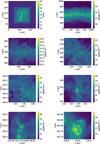 |
Fig. 1 Top-left panel: AMR level used to perform the calculation in one quarter of the computing box. The zooming strategy is clearly visible. The first levels use nearly uniform refinement while the last ones are based on the Jeans length and follow the dense gas. Top-right panel: column density for the whole computing box and along the x-axis. Second, third and fourth rows display a series ofzooms, going from 250 to 0.25 pc, showingthe column density along the y-axis. From the bottom rows, the interest and limit of the calculation clearly appear. The cores as entities are reasonably described but their internal structure is poorly described. |
3 Structure extraction and properties
3.1 HOP algorithm
The main goal of the present paper is to study the prestellar cores in the context of a self-consistently generated ISM and we must proceed to their extraction. For this purpose, we use the group finding algorithm, HOP, which has been widely used in a cosmological context to detect dark matter haloes (Eisenstein & Hut 1998). This algorithm is also used in the ISM context by Bleuler & Teyssier (2014) to identify the possible location of new sink particles. HOP finds the densest neighbour of each particle, repeating the procedure this defines a path which ends when each particle is its own densest neighbour. The ensemble of particles which end at the same local density maximum is called a group. There are a few user parameters that have been found to have little influence on the final result with the notable exception of the density threshold above which particles are considered (Eisenstein & Hut 1998). Once the groups are obtained, the algorithm also offers the possibility to merge the groups, something that we do not use in the present study.
To use HOP we proceed as follows. First, we select in the simulation all the cells that have a density above 3000 cm−3, located inside the maximally refined regions (corresponding to the greensquare visible in the top-left panel of Fig. 1). These spatial coordinates and the density of these cells are then provided to the HOP algorithm, which groups them following the procedure described above. We note that as discussed below, most structures found this way are not self-gravitating and should not be classified as cores, a point to which we return below, where several criteria are being studied. The word cores will refer to structures (i.e., groups of cells identified by HOP) which satisfy a specific criterion (typically based on virial analysis).
We note that at this stage, we do not attempt to define and extract the cores as the observers do. The reason is that this is in itself a challenging process, which requires several steps including a modelisation of the observations themselves as well as the usage of specific software (Men’shchikov et al. 2012). This goes beyond the scope of the present paper, which focuses on the method and the physical analysis of the structures formed.
3.2 Computed quantities
Once we get the groups of cells, we calculate the mass M, the velocity dispersion, σ, the cloud radius, R, the virial α parameter and the mass-to-flux over critical mass-to-fluxratio (Mouschovias & Spitzer 1976), μ. For some of these parameters, there are several possible choices. Thespatial coordinates used in the equations below are with respect to the center of mass of each individual structure.
The internal velocity dispersion is defined as

To define the radius, we first compute the inertia matrix
 (6)
(6)
that we diagonalise giving three eigenvalues λi . We then define
 (7)
(7)
To characterize the dynamical state of the structures, we compute several values of the virial parameter, α as stated by Eq. (8). First, we compute the standard observational definition that we will refer to as α. Then we compute the exact ratio between the kinetic energy and the gravitational energy αvir. Finally, we also compute the ratio between the thermal and gravitational energy, αth.
 (8)
(8)
where gi is the gravitational field.
The mass-to-flux ratio is widely used to estimate the strength of the magnetic field with respect to gravity. To compute Φ, the magnetic flux, we first compute the cloud center of mass, then we compute the flux across the three planes parallel to xy, xz, and yz and passing through the center of mass. We then take the largest of these three fluxes. The exact definition of μ depends, in principle, on the object geometry and flux distribution; here we use the definition of Mouschovias & Spitzer (1976)
 (9)
(9)

4 Statistical properties of cores
We now turn to a description of the statistical properties of the extracted structures and cores. In this section we present the results of run Z18, that is to say with a spatial resolution up to 3.6 × 10⁻³ pc and at time 10.04 Myr.
4.1 Mass, radius, and density of structures: core selections
Figure 2 shows a series of dimensional histograms displaying various quantities as described in Sect. 3.2. Top-left panel shows the mass as a function of the radius, R. While the radii span about one decade, from 0.01 to a few 0.1 pc, the masses vary over more than four decades reaching values below 0.01 M⊙ and above 100 M⊙. At first sight this seems to suggest that the radius weakly varies with the mass. However, this is not exactly the case. From the mass-radius distribution, the structures can be divided in two main populations. First, a significant fraction of objects lies around a line starting at M ≃ 0.1 M⊙, R ≃ 0.02 pc and ending at M ≃ 10 M⊙, R ≃ 0.1 pc. This population of structures roughly follows M ∝ R3. We call it region I. The second population is located around M ≃ 10 M⊙, R ≃ 0.02 pc, which we call region II.
This second population corresponds therefore to much denser objects than the ones of the first population. This can be more clearly seen on the top-right panel that displays the mean density distribution. This latter is simply defined as the ratio of the mass structure over its total volume. The structures of region I have densities of about 104−5 cm−3 and masses of 0.1–10 M⊙. The structures corresponding to region II are at much higher density. This latter is nearly proportional to their mass.
We believe that these two types of structures should be distinguished. The first one represents structures which have not yet strongly collapsed, such as pre- and protostellar cores. The second type corresponds to objects which have collapsed and therefore, since, as explained above, we are not using sink particles, their mass has piled up on a few computing cells explaining why the density increases with their mass. These objects therefore represent young stellar objects (YSO). We note however that since merging is occurring, their distribution evolves with time and bigger objects are gradually built up. This indicates that as we are studying the statistical properties of cores, it is necessary to separate the two populations.
Based on the density distribution, we see that a simple density threshold allows us to separate them easily. To demonstrate this we have plotted the radius versus mass distribution for structures with nmean < 105 cm−3 (top-left panel of Fig. 3), where it is clear that these structures lie in region I. This is also confirmed by the distribution of the αvir parameter, which is shown for all structures (bottom-left panel of Fig. 2), structures with mean density larger than 105 cm−3 (bottom-right panel of Fig. 2), and those with mean density smaller than 105 cm−3 (middle-right panel of Fig. 3). Most structures with nmean > 105 cm−3 have αvir very close to 1 (we note that there is very little mass in structures with αvir > 1 compared to structures with αvir ≃ 1). On the contrary, the ones with nmean < 105 cm−3 have a distribution that is broader and are not heavily dominated by an αvir ≃ 1 population.
We note that the collapsed structures (with high mean density) are very compact and sometimes only a few cells across. The origin of αvir ≃ 1 is the numerical diffusion which spreads the density peak over a few grid cells, while the typical velocity dispersion that is induced by the numerical scheme is simply the virial one.
In the following we therefore distinguish between objects of various mean densities. In our simulations, only the ones with mean densities below ≃ 105 cm−3 can possiblybe considered as pre- or protostellar cores. The objects with high mean densities are subject to unphysical merging since in practice these objects should have collapsed and formed a star population. As we discuss below, their mass distribution is likely affected by this process.
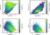 |
Fig. 2 Physical properties of all structures identified in the simulation Z18 at time 10.04 Myr. Top-left panel: mass versus radius, top-right panel: mean density versus mass. Bottom-left panel: αvir parameter (as stated by Eq. (8)) for all structures while bottom-right panel: αvir only for the structures with a mean density larger than 105 cm−3. The latter confirms that most structures with a mean density larger than 105 cm−3 are collapsed objects since αvir ≃ 1 (with little dispersion). |
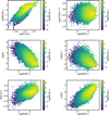 |
Fig. 3 Physical properties of structures with mean density smaller than 105 cm−3 in simulation Z18 at time 10.04 Myr (as seen with Fig. 2 these structures are not dominated by collapsed objects). Top-left panel: mass-size relation (compared with top-left panel of Fig. 2 which shows the same quantity for all structures). Top-right panel: velocity dispersion (see Eq. (4)) as a function of mass. Typical values are on the order of σ ≃ 0.3 km s−1. Second row: α and αvir . Most cores have values on the order of, or smaller than, a few. Third row: Alfvénic Mach number and the μ parameter. |
4.2 Velocity dispersion, Mach number, and virial parameter
The mass versus radius distribution for structures of densities below 105 cm−3 is displayed in the top-left panel of Fig. 3. It broadly follows an M ∝ R3 relation with masses on the order of 10 M⊙ for a radius of 0.1 pc. This is very similar with what has been inferred in the simulations of Offner et al. (2008, see their Fig. 1), more particularly their undriven case. We note that the trend M ∝ R3 is likely an artifact of the finite resolution and the density threshold of the clump finder. In particular, this relation corresponds to the lower mass object at a specific radius. As we discuss in Sect. 4.5.1, the thermally supercritical clumps, that is, the dense cores, follow a different trend that is likely not suffering from this bias.
The inner velocity dispersion of the objects with nmean < 105 cm−3 is displayed in the top-right panel of Fig. 3. The distribution is broad, it peaks around 0.5 km s−1 but extends, for few objects, above 1 and below 0.1. Since the sound speed within the dense gas is typically on the order of 0.2 km s−1, this corresponds to a Mach number on the order of 2–2.5 (not displayed here for conciseness). There is, as expected, a mild correlation between the mass and the Mach number,  (see the yellow pixels which contain most of the mass). This is also similar to the values inferred by Offner et al. (2008, their Fig. 3).
The virial parameter, αvir is displayed in the middle-right panel. As can be seen there is, as expected a large spread but most of the mass tends to lie in the vicinity of αvir on the order of, or slightly larger than, 1. Since real observations do not have access to αvir , we also estimated α using the standard definition recalled in Eq. (8). The two distributions are similar without being identical. There is a trend toward slightly larger values of α. Also its distribution is broader than the one of αvir .
4.3 Mass-to-flux ratio and Alfvénic Mach number
The Alfvénic Mach number ( ) is displayed in the bottom-left panel of Fig. 3. Typical values are ≃2 times below the Mach number ones indicating that the magnetic support dominates over the thermal one. Most objects are sub or trans-Alfvénic with very few values larger than 3. There is a clear, though shallow, trend for more massive objects to present larger
  . Typically we get
  .
.
The mass-to-flux ratio, μ, is displayed in the bottom-right panel. Objects for which μ is below 1 are magnetically subcritical and are not expected to undergo gravitational collapse at least as long as they keep their magnetic flux. As can be seen, there is a clear trend for μ to increase slightly sub-linearly with the mass, although there is a broad distribution with variation over about one order of magnitude. This behavior is significantly different from studies performed on larger-scale clumps identified through simple density thresholds (Banerjee et al. 2009; Inoue & Inutsuka 2012; Iffrig & Hennebelle 2017) where a shallower relation μ ∝ M0.4 has been reported. A simple geometrical explanation of this relation has been proposed by Iffrig & Hennebelle (2017).
The origin of this difference of behavior between the self-gravitating cores and the diffuse clouds is not obvious. Strictly speaking it implies that the magnetic flux is roughly constant through the selected structures or increases very mildly with the mass. Since the surface is proportional to R2 and therefore increases with the mass, this means that for dense cores, the magnetic field decreases with their mass. The most likely explanation is that matter preferentially flows along the field lines, therefore leading a dependence of the mass-to-flux ratio shallower than the one of the large-scale clumps whose formation is primarily due to turbulence.
Another, not exclusive possibility is that magnetic diffusion is effective. Indeed magnetic diffusion has clearly been observed in the context of collapsing cores (Hennebelle et al. 2011; Joos et al. 2013) although only in the inner part of the cores. Since the dense structures selected by the HOP algorithm are local density maxima, there are also regions of the flow which have a high magnetic field and since turbulence is significant (being dominant over or comparable to the dominant source of support), the clumps experience a few turbulent crossing times before they collapse. We note that the possibility that numerical diffusion is playing an important role in this process cannot be ruled out although turbulent diffusion is certainly known to be acting efficiently (Lazarian & Vishniac 1999).
The values of μ indicate that most structures above one solar mass are supercritical. This certainly suggests that magnetic field plays a significant role for the star formation process since it stabilizes most of the small clumps that form, a point that we discuss further in the following. It should also be stressed that while the values of μ are typicallylarger than 1 for massive cores, most of them are still below 10 which indicates that the magnetic field still has a significant influence during the collapse (e.g., Hennebelle et al. 2011; Commerçon et al. 2011; Myers et al. 2013). In particular, magnetic fields of such intensities can play an active role in reducing the gravitational fragmentation that may occur during collapse.
4.4 Massspectra
An important statistical property regarding the prestellar cores is their mass spectrum. Indeed it has been found that the core mass spectrum is very similar in shape to the IMF (Motte et al. 1998; Alves et al. 2007; André et al. 2010; Könyves et al. 2015) and several theories assume thatthe core mass function (CMF) is at the origin of the IMF (Padoan et al. 1997; Hennebelle & Chabrier 2008; Hopkins 2012; Offner et al. 2014; Lee et al. 2017). While the link between the CMF and the IMF is still debated, the CMF provides an important statistical description of the dense and self-gravitating gas, that needs to be reproduced and understood.
Figure 4 shows several mass spectra of various ensembles of structures. The top panel displays the mass spectrum of all structures identified by the HOP algorithm inthe simulation and with at least 100 computing cells. For reference, the solid lines indicate the mass spectra d N∕d logM ∝ M−1 and d N∕d logM ∝ M−1.3. The mass spectrum of all structures ranges from masses of about 0.01 M⊙ to masses larger than 103 M⊙. The high mass part (above 10 M⊙) presents a clear M−1 tail. The low mass part peaks at about 0.1 M⊙ and then steeply drops.
As seen from Figs. 2 and 3, many structures are not gravitationally bound or have already collapsed and should not be considered as prestellar cores. Therefore we also show the mass spectra of various sub-populations. The middle-left panel shows the mass spectrum of structures that have a mass-to-flux ratio, μ, smaller than 1, that is, subcritical structures, while the middle-right panel shows the mass spectrum of super-critical cores (black lines) and cores with μ >0.3. Clearly the μ parameter controls the peak of the magnetized core distribution.The subcritical structures present a peak at about 0.2 M⊙ and do not present a power-law distribution at high mass. Instead its shape is roughly lognormal. We caution that, as already discussed, the definition and therefore the physical meaning of many subcritical clumps, should be regarded with care. The peak in particular depends on the numerical resolution. On the contrary, supercritical cores (with μ >1) have a mass spectrum which peaks at about 2 M⊙ and present a high mass tail ∝ M−1. Unsurprisingly the peak shifts toward smaller mass for larger values of μ.
To remove the collapsed cores discussed in the previous section, we have selected supercritical cores for which nmean < 105 cm−3 (bottom-left panel, black line) and nmean < 106 cm−3 (bottom-left panel, blue line). The low-mass part is nearly identical to the supercritical core mass spectrum displayed in the middle-right panel but the high-mass tail is quite different. It is still a power-law but is much closer to being ∝ M−1.3 than ∝ M−1.
Finally, we have also plotted the mass spectra for thermally supercritical cores, that is to say for which αth < 1, keeping again the ones for which nmean < 105 cm−3 (black line of bottom-right panel) and nmean < 106 cm−3 (blue line). The motivation is twofold. First of all as already mentioned, ambipolar diffusion is not included and could reduce the magnetic flux, second of all, observationally it is hard to measure the magnetic intensity and for this reason thermal support is usually considered to select gravitationally bound cores. As can be seen, the shape of the high-mass part is identical to the supercritical cores. Both mass spectra peak at about 1–2 M⊙. There are however more small cores in the thermally supercritical distribution than in the magnetically supercritical one and the former is slightly broader than the latter.
Altogether these results are reminiscent of the CMFs that have been observationally obtained. In particular André et al. (2010) found that in the Gould Belt survey, the CMF peaks around or slightly below 1 M⊙ and presents a power-law ∝ M−1.3 at high mass. On the contrary, the mass spectrum of the structures observed in the Polaris cloud, which are not self-gravitating, peaks at smaller mass and has a lognormal shape. This is reminiscent of the mass spectra obtained here. The mass spectrum of subcritical structures (middle-left panel) resembles the Polaris one and the mass spectrum of supercritical ones (bottom-left panel) is similar to the CMF obtained for the Gould Belt although the observational CMF may peak at a value ≃2−3 smaller than the one inferred from the simulation (but see Sect. 6.2 for a discussion on possible numerical convergence issues).
Our results are also reminiscent of some of the CMFs previously obtained in numerical simulations (Klessen et al. 1998; Klessen & Burkert 2001; Gong & Ostriker 2015) that also present a peak and powerlaws at high masses. We stress however that since these studies are isothermal, the core masses can be freely normalized. In the present simulation, cooling is treated, and more generally the density distribution is a consequence of several processes, such as the disc vertical equilibrium itself related to the momentum injected by the supernovae.
While this is encouraging, it is important to stress that there may be difficult issues however regarding the numerical resolution and the dependence of the peak position on it, something that we discuss in Sect. 6.2.
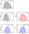 |
Fig. 4 Mass spectra of the extracted cores at time 10.04 Myr in simulation Z18. Top panel: no selection applied. Second panel: only subcritical cores, that is, those with μ < 1 are displayed. Third panel supercritical cores (μ > 1, solid line) and cores with μ > 0.3 (red dashed line). Bottom panel supercritical cores with central densities smaller than 105 cm−3 and 106 cm−3 (respectively black and blue solid curves). |
4.5 Properties of thermally supercritical cores
As our main interest is the supercritical cores, we now specifically investigate some of their properties.
4.5.1 Mass-radius of thermally supercritical cores
The upper panel of Fig. 5 shows the mass-radius relation for the thermally supercritical cores. Apart for the very-low-mass ones, the distribution is broadly encompassed between M ∝ R for the most massive objects at a specific radius and M ∝ R2 for the less massive ones, though the dispersion is quite large for logR below –1.5. The overall distribution is broadly similar to the one inferred by Könyves et al. (2015, see their Fig. 7).
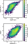 |
Fig. 5 Upper panel: mass-radius relation of thermally supercritical cores. Lower panel: magnetic mass-to-flux of thermally supercritical cores. While massive cores are all magnetically supercritical, there is a significant number of intermediate- and low-mass cores, which are magnetically dominated. |
4.5.2 Mass-to-flux ratio of thermally supercritical cores
We now examine the correspondence between the thermally and magnetically supercritical cores. For that purpose we study the distribution of the mass-to-flux ratio, μ, for cores having αth < 1 and mean density below 105 cm−3. The lower panel of Fig. 5 displays the result. As can be seen, while most massive cores are clearly magnetically supercritical (i.e., have μ >1), this is less the case for low- and intermediate-mass cores for which a significant fraction are actually dominated by magnetic field. While this result was expected since the mass spectrum of thermally supercritical cores is broader than the mass spectrum of magnetically supercritical ones, this nevertheless illustrates the difficulty of defining exactly what a core is. Indeed, a thermally subcritical object may accrete more mass or be compressed and this could make it gravitationally unstable. Similarly magnetically subcritical cores may accrete mass along the field lines orlose some magnetic flux through ambipolar diffusion if it is held by external pressure for a few diffusion times.
We must highlight that we have not included kinetic energy in the core selection, which may make some of the thermally supercritical cores stable. The reason is that in this process, one should carefully distinguish between collapsing motionthat should not be counted as kinematic support but rather counted negatively. This would require careful analysis, something beyond the scope of the present paper. Qualitatively, the mass spectrum is similar but the peak position is even more uncertain.
Observationally, Crutcher (2012) inferred that most cores are supercritical while only a few appears to be subcritical. While this may simply be an effect of selected samples (most of the selected observed cores may have already formed an object or are on the verge of doing so while our “subcritical” cores simply expand without forming an object), this may also possibly indicate that either ambipolar diffusion should be included as it is playing a significant role at the scale on the order of 0.1 pc, or the magnetic field is slightly too high in the present simulations.
4.5.3 Angular momentum
Angular momentum is an essential quantity in the context of core collapse and disc formation and we therefore investigate its distribution in our core population. The specific momentum is given by
 (10)
(10)
Figure 6 shows its distribution for supercritical cores with mean density below 106 cm−3. The upper panel displays its value as a function of mass while the bottom one shows it as a function of the velocity dispersion. As can be seen, the inferred values go from 10−3 to 10−1 pc km s−1 and scale with the mass roughly as M2∕3. These values are in excellent agreement with what has been inferred from observations (see for example Fig. 7 of Belloche 2013). They are also compatible with previous simulations such as the ones performed by Offner et al. (2008, their Fig. 5) and Dib et al. (2010, their Fig. 13).
Interestingly, the correlation between J and σ is slightly better than between J and M. This is in good agreement with the idea that the rotation of pre- and protostellar cores is primarily inherited from their initial turbulence.
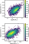 |
Fig. 6 Distribution of angular momentum in magnetically supercritical cores of mean density below 106 cm−3; the top panel displays this as a function of the mass while bottom panel shows it as a function of internal velocity dispersion. |
5 Environmental dependencies
So far we have considered the statistics for all the extracted cores present in the simulation. An important question is to what extent the core properties may vary from region to region. Given the relatively large simulated volume, there is indeed a wide range of physical conditions. To tackle this question, wehave selected five subregions of the simulation Z18 at time 10.04 Myr as displayed in Fig. 7. These regions contain many cores, therefore statistics can be drawn.
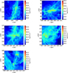 |
Fig. 7 Column density for the five selected sub-regions. |
5.1 Physical characteristics
First we quantify key physical characteristics of the selected sub-regions. Figure 8 displays the density PDF, the mass distribution or, equivalently, the mass-weighted density PDF, and the magnetic intensity as a function of density in the five sub-regions as well as in the whole fully refined zoom region.
As displayed by the top panel, the five regions present very different masses going from a few 104 M⊙ (region 1) to about 100 M⊙ (region 5). They present density PDF (middle panels) that have similar shape. They peak at low densities around 10 to 100 cm−3 (1 cm−3 for the whole refined region) and a powerlaw ≃ ρ−1 − ρ−1.5 at high density. Similar distributions have been found to be typical of gravitational collapse (Kritsuk et al. 2011; Hennebelle & Falgarone 2012; Girichidis et al. 2014). The less massive subregions (5) present however significant deviations at high densities, possibly indicating that they contain less collapsed objects.
The mean magnetic intensity is displayed as a function of density in the bottom panel. For the whole region, the usual behavior (Troland & Heiles 1986; Hennebelle et al. 2008; Banerjee et al. 2009; Crutcher 2012) is recovered, that is to say B weakly depends on n for n < 103 cm−3, where typical magnetic intensities are ≃10 μG, while at densities n > 104 cm−3,  . Let us remind that this behavior is a simple consequence of the magnetic and gravitational forces. In the diffuse gas, gravity is not dominant and the gas must flow along the field lines to avoid high magnetic pressure. On the contrary, in the dense gas, gravity can compensate for the high magnetic pressure (Hennebelle et al. 2008). For subregions 1, 2 and 3, a similar behavior is inferred, although regions 2 and 3 present values of B at low densities that are 3–10 times higher. This is due to the fact that the magnetic field has been globally compressed by gravity in these regions. Subregions 4 and 5 present a slightly different behavior at high densities, particularly region 5, that presents magnetic intensity values 2–3 times below the others.
We conclude that while the five subregions present rather different masses, their physical conditions are more similar, except subregion 5, which presents lower magnetic intensities.
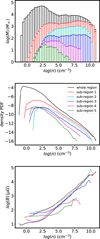 |
Fig. 8 Top panel: mass distribution as a function of density (mass weighted density PDF), bottom panel: mean magnetic intensity as a function of density for the five sub-regions shown in Fig. 7. |
5.2 Mass spectra of the sub-regions
Figure 9 shows the CMF for the whole region and the five subregions. The top panel shows the magnetically supercritical cores while the bottom one displays the thermally supercritical cores.
Subregions 1 and 2 present mass spectra that are relatively similar to the whole region one. The peak is approximately at the same place, and the shape of the high-mass part of the distribution also resembles the CMF of the whole region.
Subregion 3 presents more fluctuations, which is expected since it contains less cores. Its CMF is nevertheless similar to the ones of regions 1 and 2.
Subregions 4 and 5 present more systematic deviations. There is an excess of low-mass magnetically supercritical cores (top panel) of subregion 5 (which peaks at about 0.3 M⊙) as well as a paucity of high-mass cores. A similar behavior is observed for thermally supercritical cores of region 5. This is entirely consistent with the magnetic intensity distribution discussed above. Subregion 4 also shows an excess of thermally supercritical cores but not of magnetically supercritical cores.
Altogether these results suggest that the core properties (note that only the mass distribution has been displayed here for conciseness but similar results are obtained for the other ones) do notfluctuate very strongly from one region to another providing the region is massive enough. We note that this lack of strong variation is particularly important in the context of the apparent universality of the IMF (e.g., Bastian et al. 2010)since cores are believed to be the mass reservoir of stars; although the links between the IMF and the CMF are still debated. At first sight these weak variations are not straightforward to understand because there is a broad range of density, velocity dispersion, and magnetic field in the zoomed region. We believe that the limited variations ofthe CMF may be a consequence of the virial dynamical equilibrium that naturally develops in a collapsing turbulent clump, and tends to self-regulate the initial conditions of star forming clumps as proposed by Lee & Hennebelle (2016a,b). In particular, the effects of the density and velocityvariations onto the CMF tend to compensate each other within such regions (Hennebelle 2012; Lee & Hennebelle 2016b).
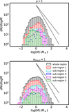 |
Fig. 9 CMF at time t = 10 Myr for the Z18 simulations and for five sub-regions. |
6 Time evolution and numerical convergence
In this section, we discuss the robustness of the results presented above. Indeed the zooming strategy may introduce biases such as a dependence on the time at which zooming starts or on the zooming strategy itself. Here we investigate in detail the evolution of the statistics with time as well as the impact of the maximum resolution reached in the simulations on the statistics.
6.1 Time evolution
Figure 10 shows the CMF (the top panel uses the μ parameter while the bottom one uses αtherm, for both of them nmean < 105 cm−3) for four time steps of the Z18 simulation. The difference between the first andthe last time step presented is about 4 Myr, which represents about one freefall time for a gas density of 100 cm−3. This therefore implies that gas typically denser than 103 cm−3 at 5.841 Myr will have experienced about 4 dynamical times by 10.04 Myr. Thus the early cores present at 5.841 Myr have collapsed at 10.04 Myr, while the early cores present at 10.04 Myr are made out of gas that was diffuse enough at 5.841 Myr. By comparing the CMF at these two times, and more generally the CMF evolution, we can therefore investigate to what extent the CMF we infer depends on the zooming time and on the zooming strategy.
The first time step (t =5.841 Myr) is only 0.2 Myr after the full refinement starts, that is to say refinement based on Jeans length up to level l = 18. As can be seen there is a visible evolution between t = 5.841 and 6.832 Myr for small objects. In particular the peak for the CMF based on μ is shifting by a factor ≃2. At a later time, we see that the number of objects increases by a factor of the order of 2 but that the shape of the distribution does not evolve significantly. Since these objects form a few millions years after the full resolution starts, this clearly indicates that the starting time does not drastically affect the statistics of the cores.
The zooming strategy is likely responsible for the difference between t = 5.841 and t = 6.832 Myr. However since there is no strong evolution of the shape at a later time, the zooming strategy we used seems to lead quickly to results equivalent to those obtained with full refinement.
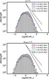 |
Fig. 10 CMF for simulation Z18 at different timesteps. |
6.2 The issue of numerical convergence
Finally, we investigate the influence of the numerical convergence, which is a central issue for the CMF. Figure 11 shows the CMF for Z17, Z18 and Z19 at comparable times, that is, 0.8 Myr after the beginning of full refinement, which was the latest we could achieve for the Z19 run. There is however a difficult point here. As discussed previously the mean density threshold is playing an important role to remove the collapsed objects. However, resolution obviously affects the mean density of collapsed objects, which increases as d x−3, where dxis the finest spatial resolution. This implies that the threshold density should increase by a factor 8 when the maximum resolution improves by a factor 2 (for example from level 18 to level 19). Therefore two thresholds are used for Z17 and Z19 runs. The dashed lines show the CMF for cores with mean density below 105 cm−3 while the solid lines show the CMF with a threshold of 106 cm−3 for Z19, 105 cm−3 for Z18 and 104 cm−3 for Z17.
As can be seen, the CMF of the Z17, Z18 and Z19 simulations with a mean density threshold of 105 cm−3, are quite different. They peak at 5, 1 and 0.2 M⊙, respectively. This is expected since smaller structures are more numerous when the resolution is higher. However the CMF of the Z17, Z18 ad Z19 simulations with threshold respectively equal to 104, 105 and 106 cm−3 are much closer and peak at about 2, 1.5 and 1 M⊙, respectively. Interestingly the high-mass part of the three CMF are also close with differences of about a factor 2. The differences are more pronounced for the thermally supercritical cores.
It is thus not possible to conclude at this stage whether or not the numerical convergence has been reached. Clearly many cores have pronounced internal structure and defining unambiguously what a core is may be an elusive task. The question as to whether the CMF will eventually converge is therefore not straightforward, although Gong & Ostriker (2015) seem to achieve numerical convergence in their simulations (see their Fig. 10). It may eventually depend on the small-scale processes that determine whether cores fragment or not.
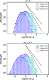 |
Fig. 11 CMF for three numerical resolutions, simulations Z17, Z18 and Z19. |
7 Conclusion
We have carried out zooming simulations using self-consistently generated initial conditions from a self-regulated supernova ISM at the kpc scale. Our strategy consists in performing a series of concentric uniform refinement and then for the last levels using the Jeans length as a refinement criterion. The spatial resolution goes up to a few 10−3 pc which is enough to describe the formation of cores of masses on the order of a few 0.1 M⊙. We identify the cores using a clump finder, requiring that the structures are thermally or magnetically supercritical. Since the domain where full refinement is applied extends over 100 pc, we get a few thousand cores providing reliable statistics. The inferred CMF present clear similarities with the observed ones. In particular, the massive objects present a power law with an exponent close to − 1.3, similar to the IMF. The peak of the CMF is found to be located around 1–2 M⊙, also similar to the observations (though possibly higher by a factor 2–3). Its position may however vary with the resolution and the significance of this peak must therefore be confirmed by future studies. Other statistics such as the velocity dispersion, the angular momentum, and the magnetization also present encouraging agreements. For instance, as in the observation, the velocity dispersion in cores is typically sonic or mildly supersonic. The angular momentum increases with the core radius and typical values are on the order of 10−2 pc km s−1. The magnetization is significant, most cores having a mass-to-fluxratio in the range 0.3 to 3. The statistics do not vary significantly with time, seemingly suggesting that the zooming procedure used in this paper does not introduce severe biases.
Acknowledgments
I thank the anonymous referee for a report that helped to improve the manuscript. I thank Philippe André for a critical reading of the manuscript as well as Juan Soler, Eva Ntormousi, Sam Geen and Damien Chapon for related discussions. This work was granted access to HPC resources of CINES under the allocation x2014047023 made by GENCI (Grand Equipement National de Calcul Intensif). This research has received funding from the European Research Council under the European Community’s Seventh Framework Programme (FP7/2007-2013 Grant Agreement No. 306483). We acknowledge PRACE for awarding us access to resource CURIE based in France at TGCC.
References
- Alves, J., Lombardi, M., & Lada, C. J. 2007, A&A, 462, L17 [NASA ADS] [CrossRef] [EDP Sciences] [Google Scholar]
- André, P., Men’shchikov, A., Bontemps, S., et al. 2010, A&A, 518, L102 [NASA ADS] [CrossRef] [EDP Sciences] [Google Scholar]
- Audit, E., & Hennebelle, P. 2005, A&A, 433, 1 [NASA ADS] [CrossRef] [EDP Sciences] [Google Scholar]
- Banerjee, R., Vázquez-Semadeni, E., Hennebelle, P., & Klessen, R. S. 2009, MNRAS, 398, 1082 [NASA ADS] [CrossRef] [Google Scholar]
- Bastian, N., Covey, K. R., & Meyer, M. R. 2010, ARA&A, 48, 339 [NASA ADS] [CrossRef] [Google Scholar]
- Belloche, A. 2013, in EAS Pub. Ser. 62, eds. P. Hennebelle, & C. Charbonnel, 25 [NASA ADS] [CrossRef] [EDP Sciences] [Google Scholar]
- Bleuler, A., & Teyssier, R. 2014, MNRAS, 445, 4015 [NASA ADS] [CrossRef] [Google Scholar]
- Burkhart, B., Lazarian, A., Balsara, D., Meyer, C., & Cho, J. 2015, ApJ, 805, 118 [NASA ADS] [CrossRef] [Google Scholar]
- Butler, M. J., Tan, J. C., & Van Loo S. 2015, ApJ, 805, 1 [NASA ADS] [CrossRef] [Google Scholar]
- Chen, C.-Y., & Ostriker, E. C. 2014, ApJ, 785, 69 [NASA ADS] [CrossRef] [Google Scholar]
- Commerçon, B., Hennebelle, P., & Henning, T. 2011, ApJ, 742, L9 [NASA ADS] [CrossRef] [Google Scholar]
- Crutcher, R. M. 2012, ARA&A, 50, 29 [NASA ADS] [CrossRef] [Google Scholar]
- Dale, J. E., Ercolano, B., & Bonnell, I. A. 2013, MNRAS, 430, 234 [NASA ADS] [CrossRef] [MathSciNet] [Google Scholar]
- Dale, J. E., Ngoumou, J., Ercolano, B., & Bonnell, I. A. 2014, MNRAS, 442, 694 [NASA ADS] [CrossRef] [MathSciNet] [Google Scholar]
- de Avillez, M. A., & Breitschwerdt, D. 2005, A&A, 436, 585 [NASA ADS] [CrossRef] [EDP Sciences] [Google Scholar]
- Dib, S., Hennebelle, P., Pineda, J. E., et al. 2010, ApJ, 723, 425 [NASA ADS] [CrossRef] [Google Scholar]
- Eisenstein, D. J., & Hut, P. 1998, ApJ, 498, 137 [NASA ADS] [CrossRef] [Google Scholar]
- Federrath, C. 2015, MNRAS, 450, 4035 [NASA ADS] [CrossRef] [Google Scholar]
- Fromang, S., Hennebelle, P., & Teyssier, R. 2006, A&A, 457, 371 [NASA ADS] [CrossRef] [EDP Sciences] [Google Scholar]
- Gatto, A., Walch, S., Low, M.-M. M., et al. 2015, MNRAS, 449, 1057 [NASA ADS] [CrossRef] [Google Scholar]
- Geen, S., Hennebelle, P., Tremblin, P., & Rosdahl, J. 2015, MNRAS, 454, 4484 [NASA ADS] [CrossRef] [Google Scholar]
- Geen, S., Hennebelle, P., Tremblin, P., & Rosdahl, J. 2016, MNRAS, 463, 3129 [NASA ADS] [CrossRef] [Google Scholar]
- Geen, S., Soler, J. D., & Hennebelle, P. 2017, MNRAS, 471, 4844 [NASA ADS] [CrossRef] [Google Scholar]
- Gent, F. A., Shukurov, A., Fletcher, A., Sarson, G. R., & Mantere, M. J. 2013, MNRAS, 432, 1396 [NASA ADS] [CrossRef] [Google Scholar]
- Girichidis, P., Konstandin, L., Whitworth, A. P., & Klessen, R. S. 2014, ApJ, 781, 91 [NASA ADS] [CrossRef] [Google Scholar]
- Gong, H., & Ostriker, E. C. 2011, ApJ, 729, 120 [NASA ADS] [CrossRef] [Google Scholar]
- Gong, M., & Ostriker, E. C. 2015, ApJ, 806, 31 [NASA ADS] [CrossRef] [Google Scholar]
- Hennebelle, P. 2012, A&A, 545, A147 [NASA ADS] [CrossRef] [EDP Sciences] [Google Scholar]
- Hennebelle, P., & Chabrier, G. 2008, ApJ, 684, 395 [NASA ADS] [CrossRef] [Google Scholar]
- Hennebelle, P., & Falgarone, E. 2012, A&ARv, 20, 55 [NASA ADS] [CrossRef] [Google Scholar]
- Hennebelle, P., & Iffrig, O. 2014, A&A, 570, A81 [NASA ADS] [CrossRef] [EDP Sciences] [Google Scholar]
- Hennebelle, P., Banerjee, R., Vázquez-Semadeni, E., Klessen, R. S., & Audit, E. 2008, A&A, 486, L43 [NASA ADS] [CrossRef] [EDP Sciences] [Google Scholar]
- Hennebelle, P., Commerçon, B., Joos, M., et al. 2011, A&A, 528, A72 [NASA ADS] [CrossRef] [EDP Sciences] [Google Scholar]
- Hennebelle, P., Commerçon, B., Chabrier, G., & Marchand, P. 2016, ApJ, 830, L8 [NASA ADS] [CrossRef] [Google Scholar]
- Hill, A. S., Joung, M. R., Mac Low, M.-M., et al. 2012, ApJ, 750, 104 [NASA ADS] [CrossRef] [Google Scholar]
- Hopkins, P. F. 2012, MNRAS, 423, 2037 [NASA ADS] [CrossRef] [Google Scholar]
- Iffrig, O., & Hennebelle, P. 2017, A&A, 604, A70 [NASA ADS] [CrossRef] [EDP Sciences] [Google Scholar]
- Inoue, T., & Inutsuka, S.-I. 2012, ApJ, 759, 35 [NASA ADS] [CrossRef] [Google Scholar]
- Joos, M., Hennebelle, P., Ciardi, A., & Fromang, S. 2013, A&A, 554, A17 [NASA ADS] [CrossRef] [EDP Sciences] [Google Scholar]
- Joung, M. K. R., & Mac Low M.-M. 2006, ApJ, 653, 1266 [NASA ADS] [CrossRef] [Google Scholar]
- Kim, C.-G., Kim, W.-T., & Ostriker, E. C. 2011, ApJ, 743, 25 [NASA ADS] [CrossRef] [Google Scholar]
- Kim, C.-G., Ostriker, E. C., & Kim, W.-T. 2013, ApJ, 776, 1 [NASA ADS] [CrossRef] [Google Scholar]
- Klessen, R. S., & Burkert, A. 2000, ApJS, 128, 287 [NASA ADS] [CrossRef] [Google Scholar]
- Klessen, R. S., & Burkert, A. 2001, ApJ, 549, 386 [NASA ADS] [CrossRef] [Google Scholar]
- Klessen, R. S., Burkert, A., & Bate, M. R. 1998, ApJ, 501, L205 [NASA ADS] [CrossRef] [Google Scholar]
- Klessen, R. S., Ballesteros-Paredes, J., & Vázquez-Semadeni, E. 2005, in Protostars and Planets V Posters, 1286, 8415 [NASA ADS] [Google Scholar]
- Kolmogorov, A. 1941, Akademiia Nauk SSSR Doklady, 30, 301 [Google Scholar]
- Könyves, V., André, P., Men’shchikov, A., et al. 2015, A&A, 584, A91 [NASA ADS] [CrossRef] [EDP Sciences] [Google Scholar]
- Korpi, M. J., Brandenburg, A., Shukurov, A., Tuominen, I., & Nordlund, Å. 1999, ApJ, 514, L99 [NASA ADS] [CrossRef] [Google Scholar]
- Kritsuk, A. G., Norman, M. L., & Wagner, R. 2011, ApJ, 727, L20 [NASA ADS] [CrossRef] [Google Scholar]
- Kudoh, T., & Basu, S. 2008, ApJ, 679, L97 [NASA ADS] [CrossRef] [Google Scholar]
- Kudoh, T., & Basu, S. 2011, ApJ, 728, 123 [NASA ADS] [CrossRef] [Google Scholar]
- Kuijken, K., & Gilmore, G. 1989, MNRAS, 239, 605 [NASA ADS] [CrossRef] [Google Scholar]
- Lazarian, A., & Vishniac, E. T. 1999, ApJ, 517, 700 [NASA ADS] [CrossRef] [Google Scholar]
- Lee, Y.-N., & Hennebelle, P. 2016a, A&A, 591, A30 [NASA ADS] [CrossRef] [EDP Sciences] [Google Scholar]
- Lee, Y.-N., & Hennebelle, P. 2016b, A&A, 591, A31 [NASA ADS] [CrossRef] [EDP Sciences] [Google Scholar]
- Lee, Y.-N., Hennebelle, P., & Chabrier, G. 2017, ApJ, 847, 114 [NASA ADS] [CrossRef] [Google Scholar]
- Li, P. S., McKee, C. F., Klein, R. I., & Fisher, R. T. 2008, ApJ, 684, 380 [NASA ADS] [CrossRef] [Google Scholar]
- Masson, J., Chabrier, G., Hennebelle, P., Vaytet, N., & Commerçon B. 2016, A&A, 587, A32 [NASA ADS] [CrossRef] [EDP Sciences] [Google Scholar]
- Men’shchikov,A., André, P., Didelon, P., et al. 2012, A&A, 542, A81 [NASA ADS] [CrossRef] [EDP Sciences] [Google Scholar]
- Motte, F., Andre, P., & Neri, R. 1998, A&A, 336, 150 [NASA ADS] [Google Scholar]
- Mouschovias, T. C., & Spitzer, Jr., L. 1976, ApJ, 210, 326 [NASA ADS] [CrossRef] [Google Scholar]
- Myers, A. T., McKee, C. F., Cunningham, A. J., Klein, R. I., & Krumholz, M. R. 2013, ApJ, 766, 97 [NASA ADS] [CrossRef] [Google Scholar]
- Ntormousi, E., Hennebelle, P., André, P., & Masson, J. 2016, A&A, 589, A24 [NASA ADS] [CrossRef] [EDP Sciences] [Google Scholar]
- Offner, S. S. R., Klein, R. I., & McKee, C. F. 2008, ApJ, 686, 1174 [NASA ADS] [CrossRef] [Google Scholar]
- Offner, S. S. R., Clark, P. C., Hennebelle, P., et al. 2014, Protostars and Planets VI (Tucson: University of Arizona Press), 53 [Google Scholar]
- Padoan, P., Nordlund, A., & Jones, B. J. T. 1997, MNRAS, 288, 145 [NASA ADS] [CrossRef] [Google Scholar]
- Padoan, P., Haugb∅lle, T., & Nordlund, Å. 2014, ApJ, 797, 32 [NASA ADS] [CrossRef] [Google Scholar]
- Seifried, D., Walch, S., Girichidis, P., et al. 2017, MNRAS, 472, 4797 [NASA ADS] [CrossRef] [Google Scholar]
- Slyz, A. D., Devriendt, J. E. G., Bryan, G., & Silk, J. 2005, MNRAS, 356, 737 [NASA ADS] [CrossRef] [Google Scholar]
- Sutherland, R. S., & Dopita, M. A. 1993, ApJS, 88, 253 [NASA ADS] [CrossRef] [Google Scholar]
- Teyssier, R. 2002, A&A, 385, 337 [NASA ADS] [CrossRef] [EDP Sciences] [Google Scholar]
- Tilley, D. A., & Balsara, D. S. 2011, MNRAS, 415, 3681 [NASA ADS] [CrossRef] [Google Scholar]
- Troland, T. H., & Heiles, C. 1986, ApJ, 301, 339 [NASA ADS] [CrossRef] [Google Scholar]
- van Loo, S., Falle, S. A. E. G., Hartquist, T. W., & Barker, A. J. 2008, A&A, 484, 275 [NASA ADS] [CrossRef] [EDP Sciences] [Google Scholar]
- Vázquez-Semadeni, E., Kim, J., Shadmehri, M., & Ballesteros-Paredes, J. 2005, ApJ, 618, 344 [NASA ADS] [CrossRef] [Google Scholar]
- Walch, S. K., Whitworth, A. P., Bisbas, T., Wünsch, R., & Hubber, D. 2012, MNRAS, 427, 625 [NASA ADS] [CrossRef] [Google Scholar]
- Wang, P., Li, Z.-Y., Abel, T., & Nakamura, F. 2010, ApJ, 709, 27 [NASA ADS] [CrossRef] [Google Scholar]
- Ward-Thompson, D., André, P., Crutcher, R., et al. 2007, Protostars and Planets V (Tucson: University of Arizona Press), 33 [Google Scholar]
All Tables
All Figures
|
Fig. 1 Top-left panel: AMR level used to perform the calculation in one quarter of the computing box. The zooming strategy is clearly visible. The first levels use nearly uniform refinement while the last ones are based on the Jeans length and follow the dense gas. Top-right panel: column density for the whole computing box and along the x-axis. Second, third and fourth rows display a series ofzooms, going from 250 to 0.25 pc, showingthe column density along the y-axis. From the bottom rows, the interest and limit of the calculation clearly appear. The cores as entities are reasonably described but their internal structure is poorly described. |
| In the text | |
|
Fig. 2 Physical properties of all structures identified in the simulation Z18 at time 10.04 Myr. Top-left panel: mass versus radius, top-right panel: mean density versus mass. Bottom-left panel: αvir parameter (as stated by Eq. (8)) for all structures while bottom-right panel: αvir only for the structures with a mean density larger than 105 cm−3. The latter confirms that most structures with a mean density larger than 105 cm−3 are collapsed objects since αvir ≃ 1 (with little dispersion). |
| In the text | |
|
Fig. 3 Physical properties of structures with mean density smaller than 105 cm−3 in simulation Z18 at time 10.04 Myr (as seen with Fig. 2 these structures are not dominated by collapsed objects). Top-left panel: mass-size relation (compared with top-left panel of Fig. 2 which shows the same quantity for all structures). Top-right panel: velocity dispersion (see Eq. (4)) as a function of mass. Typical values are on the order of σ ≃ 0.3 km s−1. Second row: α and αvir . Most cores have values on the order of, or smaller than, a few. Third row: Alfvénic Mach number and the μ parameter. |
| In the text | |
|
Fig. 4 Mass spectra of the extracted cores at time 10.04 Myr in simulation Z18. Top panel: no selection applied. Second panel: only subcritical cores, that is, those with μ < 1 are displayed. Third panel supercritical cores (μ > 1, solid line) and cores with μ > 0.3 (red dashed line). Bottom panel supercritical cores with central densities smaller than 105 cm−3 and 106 cm−3 (respectively black and blue solid curves). |
| In the text | |
|
Fig. 5 Upper panel: mass-radius relation of thermally supercritical cores. Lower panel: magnetic mass-to-flux of thermally supercritical cores. While massive cores are all magnetically supercritical, there is a significant number of intermediate- and low-mass cores, which are magnetically dominated. |
| In the text | |
|
Fig. 6 Distribution of angular momentum in magnetically supercritical cores of mean density below 106 cm−3; the top panel displays this as a function of the mass while bottom panel shows it as a function of internal velocity dispersion. |
| In the text | |
|
Fig. 7 Column density for the five selected sub-regions. |
| In the text | |
|
Fig. 8 Top panel: mass distribution as a function of density (mass weighted density PDF), bottom panel: mean magnetic intensity as a function of density for the five sub-regions shown in Fig. 7. |
| In the text | |
|
Fig. 9 CMF at time t = 10 Myr for the Z18 simulations and for five sub-regions. |
| In the text | |
|
Fig. 10 CMF for simulation Z18 at different timesteps. |
| In the text | |
|
Fig. 11 CMF for three numerical resolutions, simulations Z17, Z18 and Z19. |
| In the text | |
Current usage metrics show cumulative count of Article Views (full-text article views including HTML views, PDF and ePub downloads, according to the available data) and Abstracts Views on Vision4Press platform.
Data correspond to usage on the plateform after 2015. The current usage metrics is available 48-96 hours after online publication and is updated daily on week days.
Initial download of the metrics may take a while.