| Issue |
A&A
Volume 610, February 2018
|
|
|---|---|---|
| Article Number | A9 | |
| Number of page(s) | 16 | |
| Section | Interstellar and circumstellar matter | |
| DOI | https://doi.org/10.1051/0004-6361/201629830 | |
| Published online | 12 February 2018 | |
The first frost in the Pipe Nebula⋆,⋆⋆,⋆⋆⋆
1 Max-Planck-Institut für extraterrestrische Physik, Giessenbachstrasse 1, 85748 Garching, Germany
e-mail: This email address is being protected from spambots. You need JavaScript enabled to view it.
2 Universitäts-Sternwarte München, Ludwig-Maximilians-Universität, Scheinerstrasse 1, 81679 München, Germany
3 Kapteyn Astronomical Institute, University of Groningen, PO Box 800, 9700 AV Groningen, The Netherlands
4 Leiden Observatory, Leiden University, PO Box 9513, 2300 RA Leiden, The Netherlands
5 Aerospace Engineering, Delft University of Technology, Kluyverweg 1, 2629 HS Delft, The Netherlands
Received: 2 October 2016
Accepted: 4 September 2017
Abstract
Context. Spectroscopic studies of ices in nearby star-forming regions indicate that ice mantles form on dust grains in two distinct steps, starting with polar ice formation (H2O rich) and switching to apolar ice (CO rich).
Aims. We test how well the picture applies to more diffuse and quiescent clouds where the formation of the first layers of ice mantles can be witnessed.
Methods. Medium-resolution near-infrared spectra are obtained toward background field stars behind the Pipe Nebula.
Results. The water ice absorption is positively detected at 3.0 μm in seven lines of sight out of 21 sources for which observed spectra are successfully reduced. The peak optical depth of the water ice is significantly lower than those in Taurus with the same AV. The source with the highest water-ice optical depth shows CO ice absorption at 4.7 μm as well. The fractional abundance of CO ice with respect to water ice is 16-6+7%, and about half as much as the values typically seen in low-mass star-forming regions.
Conclusions. A small fractional abundance of CO ice is consistent with some of the existing simulations. Observations of CO2 ice in the early diffuse phase of a cloud play a decisive role in understanding the switching mechanism between polar and apolar ice formation.
Key words: astrochemistry / ISM: clouds / ISM: individual objects: the Pipe Nebula / ISM: molecules / infrared: ISM / solid state: volatile
Based on data collected by SpeX at the Infrared Telescope Facility, which is operated by the University of Hawaii under contract NNH14CK55B with the National Aeronautics and Space Administration.
Based also on data obtained at the W.M. Keck Observatory, which is operated as a scientific partnership among the California Institute of Technology, the University of California, and the National Aeronautics and Space Administration. The Observatory was made possible by the generous financial support of the W.M. Keck Foundation.
The final reduced spectra (FITS format) are available at the CDS via anonymous ftp to cdsarc.u-strasbg.fr (130.79.128.5) or via http://cdsarc.u-strasbg.fr/viz-bin/qcat?J/A+A/610/A9
© ESO, 2018
1. Introduction
Star formation starts with a diffuse interstellar cloud that gradually condenses into a dark molecular cloud. Dense cores may form inside the dark cloud and a fraction of them eventually collapse into new stellar systems. The piled-up material locally increases the visual extinction, then photodissociation rates drop exponentially, and molecules start to thrive (e.g.,
Tielens 2005). Dust grains in the dark clouds are generally cold (<15 K; Spitzer 1998; Hocuk et al. 2017) if the clouds are devoid of active star formation. As soon as the visual extinction reaches AV = 2–3 mag, water molecules copiously form on the grain surfaces via successive hydrogenation of atomic oxygen (e.g., Aikawa et al. 2003; Hollenbach et al. 2009). Other molecules in the gas phase, in particular CO, stick onto dust surfaces, producing mixed and layered ice mantles on the grains (Chiar et al. 1995). These mantles are the hideouts of the missing molecules in the gas (e.g., Caselli et al. 1999), incubators of complex organic molecules (e.g., Vasyunin & Herbst 2013; Vasyunin et al. 2017), and adhesives that facilitate grain growth up to the size of planetesimals (e.g., Gundlach & Blum 2015).
The Spitzer Space Telescope brought a leap forward in the study of the ices in the interstellar medium (see review in Boogert et al. 2015). The superb sensitivity of the spectrograph enabled observations of faint field stars behind star-forming regions as background continuum sources (e.g., Knez et al. 2005; Chiar et al. 2011; Boogert et al. 2013). The wide wavelength coverage facilitated the comparative study of the molecules in the ice. With timely advances in laboratory experiments (e.g., Ioppolo et al. 2008; Oba et al. 2010; Noble et al. 2011) and numerical simulations (e.g., Aikawa et al. 2003; Taquet et al. 2012; Cuppen et al. 2013; Sipilä et al. 2013; Hocuk et al. 2016), our understanding of the formation of ices has been substantially refined. A picture that gradually emerged is the formation of the ice mantle taking place in two sequential but distinct stages (e.g., Öberg et al. 2011; Boogert et al. 2015). The first stage is characterized by a rapid formation of water ice along with CO2, which may form either by the surface reaction of CO and OH (Ruffle & Herbst 2001) or by cosmic-ray bombardment of water ice on top of carbonaceous material (Mennella et al. 2004). The second stage is the accumulation of CO ice. The catastrophic freeze-out of CO is often observed toward dense cores at the volume density above a few ×104 cm-3 (Caselli et al. 1999; Tafalla et al. 2002, 2006).
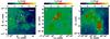 |
Fig. 1 Extinction map of the Shank in the Pipe Nebula based on the near-infrared color excess (Román-Zúñiga et al. 2010). Overlaid are the positions of the targets. The sources where water ice is positively detected are marked by yellow crosses, while those with negative detections are marked by orange crosses. The zoom-in view of the positive detections at the regions A and B are shown in the middle and right panel, respectively. |
The motivation of the present observations is to collect empirical insights into the first steps of ice formation in a quiescent molecular cloud away from the sites of active star formation without complications of (proto-)stellar feedback. Our target is the Pipe Nebula. Compared to other nearby star-forming regions such as Taurus, Lupus, and Serpens, the Pipe Nebula is clearly more quiescent. Only a handful of embedded sources are known in the entire complex, most of which are located in B 59 at the tip of the Stem (Duarte-Cabral et al. 2012; Hara et al. 2013). The sub-mm molecular lines are narrow (0.2–0.5 km s-1; Muench et al. 2007; Frau et al. 2010), indicating that the gas is mostly subsonic (Lada et al. 2008) and giving support to the early evolutionary stage of the cloud. The Pipe Nebula is located at 130–145 pc from the Sun (Lombardi et al. 2006; Alves & Franco 2007). Projection against the Galactic Bulge guarantees a large reservoir of background stars to choose from.
We illustrate in Sect. 2 how the spectroscopic data are collected, and the optical depths and the column densities of water and CO ices are extracted. The caveats in using AV as a reference of the optical depths of ice is discussed in Sect. 3.1. Possible interpretations of the observations with locally enhanced radiation field and chemical evolution of the ice are discussed in Sects. 3.2 and 3.3, respectively. The column densities of water, CO, and CO2 ice are complemented by the literature, and are compared to the latest simulations in Sect. 3.4. The summary of the present study is given in Sect. 4.
2. Observations, data reductions, and results
2.1. SpeX/IRTF
2.1.1. Observation
The near-infrared spectrograph SpeX (Rayner et al. 2003) at the IRTF on Mauna Kea is used to collect the medium resolution spectra of the field stars behind the Pipe Nebula. SpeX is equipped with a prism cross-disperser. Together with the large-format 2048 × 2048 pixel detector array, the instrument covers a wide wavelength interval with a single exposure. The wide simultaneous wavelength coverage is an integral component of the present observations; the biggest challenge in observing water ice from the ground is to constrain the short wavelength continuum properly. The stretching vibrational band of water ice is centered at 3.0 μm and the absorption profile is broad. The absorption extends beyond 2.8 μm in the short wavelength, overlapping with the atmospheric water vapor at 2.7 μm. It is therefore hard to set the continuum level correctly with the L-band spectroscopy (2.8–4.1 μm) only. Spectroscopy or photometry at the K-band (1.9–2.5 μm) can be used to set the continuum baseline, which is not only time consuming in observations, but also introduces other systematics such as variable slit throughput. Simultaneous coverage of K and L by SpeX is a critical advantage to the observational study of water ice from the ground.
All targets are from the Shank in the Pipe Nebula, where no signs of star formation have been identified to date. The stars were selected so that they collectively cover the visual extinction from AV = 3 to 12 mag (Fig. 1), referring to the extinction map of Román-Zúñiga et al. (2010). The selected targets are brighter than Ks< 9 mag in 2MASS (Skrutskie et al. 2006) and W1 < 8.6 mag (3.4 μm) in WISE photometry (Wright et al. 2010). Visually bright stars in the USNO B1.0 catalog (R< 13 mag) are filtered out, because the chances are high that they are foreground stars. The summary of the targets is given in Table 1.
Summary of targets and optical depths of ices.
The observations were carried out on eight half-nights in May and June in 2015. The instrument was remotely operated from Munich in Germany. All spectra were obtained with the optics setting LXD_long with the 0.̋8 slit. The slit was roughly aligned to the parallactic angle to reduce the loss of flux at the slit by the atmospheric refraction. The spectra were recorded by nodding the telescope along the slit every second exposure to remove the sky background emission. Early-type standard stars were observed immediately after the science targets. Spectroscopic flat field, i.e., a continuum illumination of a halogen lamp, was obtained with the same instrument setting after the observation of the standard stars. Argon lamp spectra were obtained after the flat field to map the wavelength on the detector array.
2.1.2. Extraction of spectra
The one-dimensional spectra were obtained using xSpexTool v4.1, which runs on an intuitive graphical user interface (Cushing et al. 2004). The IDL-based spectral reduction package performs flux calibration, non-linearity correction, wavelength calibration, coadding of the two-dimensional spectrograms, aperture extraction, and merging of the spectra extracted from the different diffraction orders. More detail is found on the IRTF SpeX webpage1.
The atmospheric absorption features are removed by dividing the object spectrum by that of a spectroscopic standard star. The blackbody spectra of the effective temperature of the standard star is multiplied to restore the continuum slope. The effective temperatures are taken from Allen’s Astrophysical Quantities (Cox 2000) of the corresponding spectral type documented in SIMBAD. Prominent H i absorption lines (Br γ, Pf γ, and Br α) are removed beforehand by fitting a Lorentzian function and subtracting it from the spectra. Less prominent H i lines blended with the atmospheric absorption lines (e.g., Pf δ at 3.297 μm) are removed after the object spectra are divided by the standard star spectra.
The absolute flux calibration is performed by scaling the object spectra to the broadband photometry at 2MASS Ks and WISE W1. The SpeX spectra are convolved by the 2MASS/WISE filter transmission curves before comparing to the photometry. A mean scaling factor at Ks and W1 bands is multiplied to the object spectrum without adjusting K- and L-band spectra to each other.
2.1.3. Template matching
The targets we observed are late-type stars with clear photospheric CO bandhead absorption at the 2.3 μm (Fig. A.1). Following Boogert et al. (2011), the photospheric lines are removed by comparing the object spectra with those of the spectroscopic template stars in the IRTF Spectral Library (Rayner et al. 2009). A series of template spectra are reddened by a trial AK ranging from 0.0 to 4.0 mag with a 0.01 mag step that roughly corresponds to sampling AV from 0 to 36 mag by 0.1 mag step. The empirical infrared extinction curve obtained by Boogert et al. (2011) is used. The reddened template spectrum is scaled to the continuum of the object spectrum at 3.6–4.0 μm, and the residual spectrum against the object spectrum is calculated. The combination of the template and AK that minimizes the residual spectrum is taken as a match. The template spectra themselves are slightly affected by the extinction on their own. Rayner et al. (2009) corrected the extinction in the library spectra in the case that substantial reddening is inferred in their B−V colors. The extinction corrected library spectra are used whenever available. Most of the spectra in the IRTF Spectral Library are obtained with the 0.̋3 slit, and therefore at higher spectral resolution than our observations. The library spectra are convolved before comparing to the object spectra. A small wavelength shift between the template and the observed spectra is corrected down to the order of 10-4μm.
The residual spectra are evaluated between 1.9 and 4.1 μm excluding the wavelength interval of the water ice band and the long-wavelength absorption excess (2.5–3.6 μm). The best matching template spectra are shown with the object spectra in the middle column of Fig. A.1. Out of the 46 targets observed, 21 stars match the spectral type M6 or earlier, and are used in further analysis (Table 1). The rest of the sample consists of stars later than M6, whose photospheric absorption of water vapor is too deep to be corrected by the template spectra (not shown in Fig. A.1).
2.1.4. Optical depth and column density
The optical depth is calculated as the natural logarithm of the scaled template spectra (f0) divided by the object spectra (f), i.e.,  . The optical depth spectra are fit by a Lorentzian function to measure the peak absorption depth at 3.0 μm (τ3.0). The choice of the template spectrum is a significant source of uncertainty in the optical depth. We have selected the three best matching templates and show the range of the optical depth spectra in the right panels of Fig. A.1 to highlight the systematic uncertainty that stems from the templates. In order to take into account this uncertainty, the upper and the lower margins of τ3.0 are set in such a way that the whole range of the peak optical depths calculated with the three different templates are encompassed. The standard deviation of the continuum baseline is added upon that range by a squared sum to represent the statistical part of the uncertainty. The seven sources (2, 6, 15, 1, 8, 7, 14) where the peak optical depths τ3.0 are observed with a significance larger than twice the total uncertainty are taken as positive detections (Fig. 2). The selection criterion matches the positive detections by visual inspection as well.
The equivalent widths of the water ice are calculated by scaling the ice absorption spectrum recorded in the laboratory (Hudgins et al. 1993) to the peak optical depth of the observed spectrum. The excess absorption at the long wavelength shoulder at 3.4 μm is therefore excluded from the integration of the water ice absorption. The equivalent width is converted to the unit of wavenumber cm-1 and divided by the integrated band strength A = 2.0 × 10⁻¹⁶ cm, adopted from Gerakines et al. (1995) to calculate the water ice column density N(H2O). No CO ice absorption was found in the SpeX spectra. The results are summarized in Table 1.
2.2. NIRSPEC/Keck II
2.2.1. Observation
The seven sources where water ice is positively detected at 3.0 μm by SpeX are further investigated using NIRSPEC spectrograph (McLean et al. 1998) at the Keck II telescope. One of the advantages of NIRSPEC over other infrared spectrographs on 8m class telescopes is that the instrument delivers relatively high spectral resolution with a wide slit. This is particularly useful when no wavefront reference source is available to use an adaptive optics system, as in the present case. We used a slit 0.̋72 wide and 24′′ long to attain the spectral resolution R = 15 000. Although the CO ice band is much broader (FWHM ~ 0.01 μm or R ≈ 1000 required for a Nyquist sampling), observation with a high spectral resolution is favored because it facilitates the removal of the photospheric absorption of late-type stars. The echelle and the cross-dispersing grating are set to 61.0° and 36.7° to place the spectral strip of the diffraction order 16 on the lower quadrants of the detector array with the wavelength 4.672 μm set at the center. The M-WIDE filter was put in the optical path in conjunction. The instrumental setting was fine-tuned by the NIRSPEC Echelle Format Simulator (EFS)2 in advance of the observing runs.
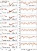 |
Fig. 2 Optical depth spectra of water (3.0 μm; left column) and CO ice (4.672 μm; right column) toward the seven sources where water ice was positively detected in the observations by SpeX spectrograph at the IRTF. The numbering of the sources in Fig. 1 and Table 1 is shown at the bottom left of the water-ice panels with the 2MASS IDs. The CO ice spectra were obtained by NIRSPEC spectrograph at Keck II. The whole SpeX spectra including negative detections are compiled in Fig. A.1. Black, red, and orange plots, are the spectra in which photospheric features are removed by referring to the best, the second best, and the third best matching M-type template stars. The visual extinctions based on the color excess (AV CE; Román-Zúñiga et al. 2010) and on the template matching with the IRTF Spectral Library (AV SpeX; Rayner et al. 2009) are shown at the bottom right of the water ice spectra. |
The observation was carried out in the first half of the nights of 6–8 August 2016 UT. The instrument was operated from Keck Headquarters in Waimea. The slit was roughly oriented to the parallactic angle at the acquisition of the target. The spectra were recorded by moving the source along the slit at every second exposure. The pointing limit of Keck II is about 37° in elevation on the southern sky3. The science targets in the Pipe Nebula were observed in the first quarter of the nights, and in total 20 M-type template stars were observed in the second quarters. The template spectra were used to remove the photospheric absorptions of the science targets. A few early-type standard stars were observed per night.
2.2.2. Extraction of spectra
The preliminary data reduction is performed using REDSPEC IDL package4. The raw frames are pair subtracted, and the pixel sensitivities are normalized by the flat field of the night. The spectral curvature and the curvature of the slit images are fit by polynomial functions and rectified. Wavelength dispersion is mapped out on the detector, referring to the sky emission lines. One-dimensional spectra are extracted from the coverture-corrected spectrograms.
The science spectra on the sources behind the Pipe Nebula, and the template spectra of nearby M-type stars are corrected for the atmospheric absorption lines by dividing by the spectra of the early-type standard stars observed through similar airmasses. Small mismatches in the wavelength solution, the spectral resolution, and the optical depths of the atmospheric lines are corrected manually. For each science target, the three best matching M-type template stars are identified on the basis of maximum cross-correlation. The selected template star spectra were used to remove the photospheric absorption lines of the science target.
2.2.3. Optical depth and column density
Fully reduced spectra are binned by 21 pixels to the spectral resolution R = 3600, and shown in Fig. 2. The optical depth of CO ice is calculated assuming that the wavelength intervals 4.645–4.655 μm and 4.685–4.700 μm are genuine continuum emission with null ice absorption. Looking at the spectra, CO ice appears to be detected on source #2 (2MASSJ 17312818−2631268). The line of sight to source #2 passes a dense core with the smallest impact parameters among the sources observed (Fig. 1), and it shows the highest water-ice optical depth in the SpeX spectroscopy. The ratio of the peak optical depth at 4.7 μm (τ4.7) and the standard deviation of the zero optical depth at the continuum is 2.6. The equivalent widths of the CO ice is estimated as  , where σ4.7 is the Gaussian sigma measured by fitting the absorption profile. The equivalent width of CO ice is converted to the column density using the integrated band strength A = 1.1 × 10⁻¹⁷ cm taken from Gerakines et al. (1995). The results are shown in Table 1.
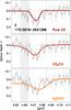 |
Fig. 3 CO ice spectra toward source #2 (17312818−2631268) recorded by NIRSPEC spectrograph. The black plot is the spectra binned by 21 pixels from the original sampling, and the gray plot by 11 pixels. The observed spectra shown in the three panels are identical. The laboratory spectra of CO ice obtained by Palumbo & Strazzulla (1993) are overlaid in red, dark orange, and light orange in each panel. The top panel shows the spectrum of CO ice deposited by itself, the middle panel CO ice deposited with CO2, and the bottom panel CO ice embedded in water ice. The dotted gray lines are the assumed continuum level with zero optical depths. The region marked in light gray indicates where the continuum level is uncertain. |
The nearby template stars are significantly blueshifted from the science targets, sometimes by as much as ~200 km s-1. A substantial part of the spectra on the short-wavelength continuum is therefore lost at the photospheric correction. With a tiny margin of continuum left, it is hard to discern if the short-wavelength shoulder 4.655–4.665 μm is part of the continuum or of the absorption feature. If we assume this interval is part of the continuum, the equivalent width of CO ice on source #2 decreases to 2/3. None of the stars other than #2 shows clear CO ice absorption at 4.7 μm. The upper limits of the optical depth on those sources are 0.09–0.16, or ~ 1017 cm-2 in the column density, with 3σ significance.
The column of CO-ice detected on source #2 is one of the smallest records observed. The column density of CO with respect to water ice is 16 %. If we take the narrow feature option discussed above, the ratio is reduced to 11%. This is smaller than the typical fractional abundance of CO ice ~30% found by Spitzer on background field stars toward nearby star-forming regions (Öberg et al. 2011). The small fractional abundance of CO ice at small column density is qualitatively consistent with the larger AV threshold for CO ice (AV = 6.0 ± 4.1; Chiar et al. 1995) than that for water ice (AV = 3.2 ± 0.1; Whittet et al. 2001).
2.2.4. Comparison with laboratory spectra
The CO ice absorption detected toward source #2 is compared to the three laboratory spectra recorded by Palumbo & Strazzulla (1993) in Fig. 3. The laboratory CO ice absorption is narrowest when deposited by itself (2.5 cm-1 or 0.006 μm in FWHM), and the absorption maxima happens at the shortest wavelength (2139 cm-1 or 4.675 μm; top panel in Fig. 3). The presence of co-adsorbate in general shifts the line center longer (2137–2135 cm-1, 4.679–4.684 μm) and broadens the line width (3.5–24 cm-1 or 0.008–0.05 μm). The effect is more prominent for co-adsorbate with a larger dipole moment (Sandford et al. 1988; Ehrenfreund et al. 1996). Co-adsorbates, or matrix, sometimes add a satellite feature at shorter wavelengths, as in the case of water (Palumbo & Strazzulla 1993). Since it is hard to tell if the shoulder of the observed depression at 4.655–4.665 μm belongs to the absorption or to the continuum, we have two distinct solutions for the line widths. The narrow line solution might well be reproduced by pure CO ice (top panel in Fig. 3), while the broader solution by the mixture of CO and CO2 (middle panel). In both cases the line center of the observed spectra (4.672–4.673 μm) matches the laboratory spectra reasonably well.
The observed CO ice absorption does not seem to agree with the laboratory spectra of CO ice mixed with H2O ice (bottom panel) where the absorption maximum happens at 4.677 μm. We note that the observed CO ice spectrum is normalized assuming that the intervals 4.645–4.655 μm and 4.685–4.712 μm are the continuum, which effectively removes any excess absorption at those wavelengths. The mixture of CO and H2O has prominent satellite feature at 4.647 μm, which is not fully covered in the astronomical spectrum. To see whether the small margin of the observed continuum biases the matching of the profiles, the laboratory spectrum of H2O:CO is reduced in the same way with the astronomical spectrum, assuming the same intervals of the continuum. The line center of the H2O:CO laboratory spectrum changes little, and the conclusion stays the same.
3. Discussion
3.1. Vistual extinction versus water ice optical depth
3.1.1. Comparison of visual extinctions
There are at least three choices of extinctions to compare with the ice optical depths: (1) the extinction measured by the color excess, which is presented in Román-Zúñiga et al. (2010) as an extinction map (AV (CE) and AK (CE) in Table 1); (2) the extinction measured by the template match using the SpeX spectra (AK(SpeX)); and (3) the extinction measured by comparing the infrared photometry of the sources with the theoretical stellar models (AK (SED)).
To obtain the extinction in method (3), the infrared photometry of the objects from 1.2 to 22 μm are collected from 2MASS and WISE catalogs. Theoretical stellar models and the SEDs are computed by the PARSEC code (Bressan et al. 2012) available through a web interface5. The theoretical SEDs are reddened by the same infrared extinction curve of Boogert et al. (2011) used at the template matching with the IRTF Spectral Library. The infrared extinction AK that best reproduces the observed SEDs are listed in Table 1 as AK (SED).
The infrared extinctions on the lines of sight obtained by the three techniques above are compared in Fig. 4. The visual extinction AV by Román-Zúñiga et al. (2010) is converted to AK by multiplying AK/AV = 0.112 (Lombardi et al. 2006). In ideal circumstances, all three extinctions should agree, which is apparently not the case.
Each technique has its advantage and disadvantage. The color excess technique does not measure the intrinsic color of the individual stars, but uses the average color of the stars in the nearby control field. The extinction is further averaged over a 20′′ square field; therefore, the technique is robust against the outliers, but at the cost of not being sensitive to individual lines of sight. Limited spatial resolution, compared to a pencil beam measurement on an individual source, may miss smaller structures with high visual extinctions. Román-Zúñiga et al. (2010) reported that the peak AV in the densest part of the Pipe Nebula increases by a factor of 4 in their extinction map; the spatial resolution is three times higher than used by Lombardi et al. (2006).
On the other hand, the critical drawback of the spectral template and the SED technique is that the extinction is biased to those sources in the Galactic Bulge far behind the Pipe Nebula. Lombardi et al. (2006) noted a clear bifurcation of the stars toward the Pipe Nebula on the near-infrared color-color diagram. The “lower branch” stars in the diagram are brighter than those in the “upper branch”, and are likely a bulge population. The apparent brightness of the lower branch stars peaks at K ≃ 7 mag, and closely matches our target selection. The line of sight to the Galactic Bulge goes through the long distance behind the Pipe Nebula, which is mostly diffuse, and not related to the ice absorption inside the Pipe Nebula. The extinction biases toward the higher AK by SpeX template (2) and SED (3) with respect to the color-excess technique (1) can be seen in Fig. 4. We therefore adopt the visual extinction obtained by the color excess method to compare with the ice optical depths, despite the risk of underestimating AV. The uncertainty of AV in the Shank is 0.33 mag according to Román-Zúñiga et al. (2010). The foreground extinction toward the Pipe Nebula is estimated to be AV = 0.12 mag by Lombardi et al. (2006) based on the color excess of the Hipparcos stars with well-defined distances, and is smaller than the uncertainty quoted above.
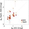 |
Fig. 4 Comparison between AK from the near-infrared color excess (CE) technique by Román-Zúñiga et al. (2010) against the SpeX templates and the SED fitting. The boxes attached to AK measured by SpeX templates delineate the range of extinctions with 3 best matching templates. The dotted line represents the case where the AK’s would be identical to the color excess. |
 |
Fig. 5 Peak optical depth of the water ice (τ3.0) plotted against the visual extinction on the line of sight (AV). The three panels are all identical, but the area shown is smaller going from left to right. The enlarged areas are shown by dotted lines in the left panels. The canonical relation between τ3.0 and AV in Taurus found by Whittet et al. (2001) is shown by dashed lines. The measurements toward the Pipe Nebula are shown by filled yellow circles. Other measurements shown in the panels are from star-forming regions such as Taurus (Whittet et al. 1988; Smith et al. 1993; Murakawa et al. 2000), Lupus (Boogert et al. 2013), and IC 5146 (the Cocoon Nebula, Chiar et al. 2011). Two starless cores, L 183 (Whittet et al. 2013), L 429 (Boogert et al. 2011), and the globules in the Southern Coalsack (Smith et al. 2002) are shown as well. The linear regression fit to the data points from the Pipe Nebula is depicted by the gray line. Filled gray circles are the same as yellow circles, but after reducing AV by 25% from those in Román-Zúñiga et al. (2010). |
The peak optical depth of water ice τ3.0 is plotted against AV in Fig. 5. A linear regression fit to the seven sources where the water ice is positively detected renders m = 0.050 ± 0.026 and the threshold extinction  mag in
  . The coefficients are not well constrained because of the short baseline of AV and the large uncertainty in τ3.0. Instead of going into a quantitative discussion on m and
  , we would like to concentrate on the apparent offset of τ3.0 from the canonical relation known in Taurus (Whittet et al. 2001). The offset can be interpreted in two ways: the visual extinction AV is too large for the given τ3.0 in the Pipe Nebula, or the optical depth of the water ice is too small for the given AV. The first possibility is discussed in the next sections. We note that the visual extinction measured by the photometric color excess adopted above is the most conservative option in this regard.
3.1.2. Conversion of color excess to AV
Whatever technique is used, the only observable we have to constrain the line of sight extinction is the color of the background sources measured either by photometric or spectroscopic means. The observed color is compared with the intrinsic color of the source, obtained either self-consistently from spectroscopy or by an educated guess such as an average color in a control field. The difference between the observed and the intrinsic color amounts to the color excess E(λ1−λ2). The color excess is converted to the extinction by Aλ = cλ·E(λ1−λ2), where cλ is the conversion factor given by an extinction law. Different authors adopt different extinction laws, thereby a different conversion factor cλ (e.g., Rieke & Lebofsky 1985; Cardelli et al. 1989; Indebetouw et al. 2005). Some extinction laws commonly used in the literature are constrained by the observations through diffuse clouds, where the stars are visible at B and V. It may well be the case that the extinction law in diffuse clouds differs from that in dense clouds because of the grain growth and the altered grain compositions (Chiar et al. 2007; Nishiyama et al. 2009). In a dense cloud with visual extinction AV ≳ 10 mag, few stars are visible, which makes it next to impossible to calibrate an infrared extinction law against the optical extinction to constrain AV/AK empirically (Indebetouw et al. 2005).
The extinction map of the Pipe Nebula by Román-Zúñiga et al. (2010), used in the present study, adopts the extinction law by Indebetouw et al. (2005) to convert the color excess to AK, and Rieke & Lebofsky (1985) to convert AK to AV, which results in AV = 6.4 E(J−K) and AV = 16.2 E(H−K). The visual extinctions used to constrain the threshold AV in Taurus (Whittet et al. 2001) were collected from diverse sources. The color-extinction conversions used are AV = 5.3 E(J−K) by Whittet et al. (1988), AV = 5.4 E(J−K) by Smith et al. (1993), AV = 12 E(H−K) by Murakawa et al. (2000), AV = 4.6 E(J−K) by Elias (1978), and Tamura et al. (1987). The conversion factor we adopt is indeed larger than those used in Taurus. If we reduce a visual extinction by Román-Zúñiga et al. (2010) by a factor of 25% to match Murakawa et al. (2000) which has the largest difference, the apparent deviation of τ3.0 in the Pipe Nebula from Taurus would almost disappear, even though all measured τ3.0 still lie below the line expected in Taurus (indicated by gray circles in Fig. 5).
This amount of uncertainty in the extinction law is entirely conceivable. Nishiyama et al. (2009) reconstructed the wavelength dependency of Aλ/AKs toward the Galactic Center, using red clump stars in the Galactic Bulge. The extinction ratio they found at H and Ks is AH/AKs = 1.69, while Román-Zúñiga et al. (2010) adopted AH/AKs = 1.55 from Indebetouw et al. (2005) constrained by the 2MASS and Spitzer GLIMPSE surveys through the Galactic plane toward l = 42° and 284°. The smaller AH/AKs of Román-Zúñiga et al. (2010) indeed increases AKs by ~25% with respect to Nishiyama et al. (2009), as 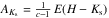 , where c = AH/AKs.
3.1.3. Diffuse components
Another way to account for the excess AV is by the anisotropic distribution of diffuse components. The threshold AV represents the presence of an outer skin where grains remain bare. The bare grains contribute to the visual extinction, but not to the optical depth of ices. We can think of two geometries that increase the relative path length through such a diffuse medium. For instance, the dense cloud could be clumpy, and the line of sight could pass through more than one dense region or dense core. Each dense core is covered by a diffuse skin; therefore, the threshold AV would increase by as much as the number of diffuse components that are along the line of sight (Smith et al. 2002). Alternatively, the line of sight might also pass only a single dense core but with various impact parameters (Murakawa et al. 2000). Supposing a spherical dense core embedded in a diffuse cloud and a line of sight that barely grazes the surface of the dense core, the fraction of the pathlength in the diffuse component would be larger than when the sightline hits the very center of the core. The contribution to AV from the diffuse component would therefore larger. Such configurations are, however, not able to explain the excess AV in the Pipe Nebula. The projected separation of the targets we observed ranges from 0.08 to 0.63 pc (Fig. 1), and is similar to or larger than the typical size of a single dense core (~0.1 pc). If the particular geometries of cloud cores are responsible for the extra visual extinction, significant scatter is expected in the excess AV in Fig. 5. On the contrary, the optical depths of the water ice line up almost in a straight line with small scatter in AV. A single constant offset in all AV prefers a common diffuse screen that covers all lines of sight.
Based on the color excess of Hipparcos and Tycho stars, Lombardi et al. (2006) dismissed the presence of such a diffuse component in front of the Pipe Nebula that contributes more than AV = 1 mag. As is discussed in Sect. 3.1.1, the targets we observed have a bias of being in the Galactic Bulge. A diffuse screen far behind the Pipe Nebula is, however, also not likely. Source #2 shows the largest τ3.0, and has the largest offset in AV from the canonical τ3.0 relation in Taurus. The infrared extinction AK toward #2 obtained by the spectral template and the SED analysis agree well with the color excess, suggesting #2 is immediately behind the Pipe Nebula. If an extra diffuse component is responsible for the enhanced visual extinction, the screen is not far away from the Pipe Nebula, but could be part of it.
3.2. Radiation field
The second interpretation of Fig. 5 is that the optical depth of the water ice in the Pipe Nebula is too small for a given AV, possibly because of the elevated interstellar radiation impinging on the Pipe Nebula. In a quiescent cloud, photoprocesses (dissociation and desorption) are the primary hindrances to ice mantle formation. Hollenbach et al. (2009) gives a succinct formula of the threshold AV for ice formation that is proportional to  , where n is the gas number density and G0 is the far-UV radiation field outside the cloud in units of Habing field (Habing 1968). A stronger radiation field implies faster photodissociation and desorption, while the higher density accelerates the accretion of molecules on the grain surface. Using the formula (17) of Hollenbach et al. (2009), the radiation field must be ~ 18 G0 to double the threshold AV from 1.6 mag (Taurus) to 3.2 mag.
The Pipe Nebula is close to ρ Oph in projection, where a large G0 is inferred by the presence of high-mass stars in the nearby Sco-Cen OB association (Wilking et al. 2008). The water ice in ρ Oph shows a similar trend to the Pipe Nebula with smaller optical depths than in Taurus at the same visual extinctions (Tanaka et al. 1990; Chiar et al. 1995). The small column density of CO ice with respect to water ice in ρ Oph (~20%; Kerr et al. 1993) may corroborate that the Pipe Nebula and ρ Oph are bathed by stronger radiation field than other nearby dark clouds.
A stronger radiation field raises the dust temperature in a cloud (e.g., Hollenbach et al. 1991; Galli et al. 2002). The dust temperatures measured in the Pipe Nebula by far-infrared imaging with Herschel are 15–19 K at AV = 10 mag (Forbrich et al. 2014). This is higher than other similar quiescent clouds such as L 1595 and B 68 (10–13 K; compilation presented in Hocuk et al. 2017). In order to raise the dust temperature to 15–19 K at the depth AV = 10 mag, the external G0 must be in the range of 25–100, according to the prescription given by Hocuk et al. (2017).
Little is known about G0 around the Pipe Nebula by non-dust UV probes. Kamegai et al. (2003) compare their [CI] observation in ρ Oph with the PDR model by Kaufman et al. (1999), and estimated G0 to be ~ 100. On the other hand, Bergin et al. (2006) argues that G0 must be 0.2 or smaller to reproduce C18O line emission at the outer part of B 68. B 68 is located between the Pipe Nebula and ρ Oph, but much closer to the former in the projection on the sky.
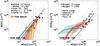 |
Fig. 6 Column densities of CO (left) and CO2 (right) ices plotted against that of water ice. The measurements of CO ice toward the Pipe Nebula are all upper limits (yellow triangles) except for 17312818−2631268 (source # 2) shown in the yellow circle. The gray circle is the column density of CO ice on source #2 as well, but measured assuming that the short-wavelength shoulder 4.655–4.665 μm is part of the continuum (see Sect. 2.2.3). No observation of CO2 ice is available in the Pipe Nebula. Other measurements shown are from Taurus (Whittet et al. 2007), L 183 (Whittet et al. 2013), CK 2 (Knez et al. 2005), IC 5146 (Q21-1; Chiar et al. 2011), assorted quiescent clouds (Noble et al. 2013), Lupus (Boogert et al. 2013), and L 429 (Boogert et al. 2011). All the measurements are against the continua of background field stars through quiescent clouds. Only those lines of sight where both CO and CO2 ices are positively detected are shown. Four simulations of ice formation are compared with the observations (Hocuk et al. (in prep.); Vasyunin & Herbst 2013; Garrod & Pauly 2011; Pauly & Garrod 2016). The number of layers presented in the simulations are converted to the column density by assuming that one monolayer corresponds to 9.6 × 1015 cm-2 (Appendix B). Model column densities calculated with conversion factors that are two times larger and smaller are shown by the shaded areas. |
3.3. Ice mantle in formation
Another possible explanation of the small optical depth of water ice in the Pipe Nebula is that the formation of the ice mantle has just started. The optical depths of the water ice in nearby star-forming regions, Taurus, Lupus, and IC 5146 (the Cocoon Nebula), and in the starless cores L 183, L 429, and the globules in the Southern Coalsack, are plotted in Fig. 5 along with the present observation in the Pipe Nebula. This is not an exhaustive survey, but the recent spectroscopy by the Spitzer Space Telescope are selected with priority. The optical depth of the water ice in the Pipe Nebula is lower than that in Taurus at the same AV (Whittet et al. 1988; Smith et al. 1993; Murakawa et al. 2000), although many sightlines in Taurus are also in quiescent parts of the cloud. The optical depth of water ice in Lupus (Boogert et al. 2013) and IC 5146 (Chiar et al. 2011) aligns well with Taurus. The good correlation between AV and τ3.0 in star-forming regions implies that these environments are old enough for the growth of the ice mantle to have reached steady state. The ice column density increases proportional to AV, implying that this is due to the accumulation of the mass along the line of sight, rather than to the formation of more ice mantles.
L 183 (Whittet et al. 2013) and L 429 (Boogert et al. 2011) are evolved starless cores (prestellar cores, Crapsi et al. 2005) with no active star formation spotted currently. The water ice optical depths in L 183 and L 429 are not too different from those in Taurus. The visual extinction toward L 183 at the far-infrared continuum peak reaches ~150 mag (Pagani et al. 2004). L 429 is seen in absorption against background continuum emission up to the wavelength 70 μm by MIPS on Spitzer (Stutz et al. 2009). The visual extinction at the core center reaches 35–130 mag. The large visual extinction implies that both starless cores are in a physically evolved phase and on the verge of starting star formation.
On the contrary the largest visual extinction in the Southern Coalsack found by the near-infrared color excess technique is AV ~ 12 mag (Lada et al. 2004), which is similar to or less than the maximum extinction in the Shank of the Pipe Nebula (AV ~ 15 mag; Román-Zúñiga et al. 2010). Smith et al. (2002) reported that the optical depth of water ice is significantly lower than Taurus at the same AV, similar to the Pipe Nebula, but in a more extreme manner (right panel of Fig. 5). All alternative explanations discussed in Sect. 3.1 also apply to the Southern Coalsack; however, the correction in AV required to align the observation in the Southern Coalsack to Taurus is ~5 mag, or ~50% reduction of AV, which is not easy to justify even with typical uncertainties in the extinction laws. It is intriguing that among the many sightlines observed, the two clouds that are possibly at the earliest stage of evolution show the lowest τ3.0.
3.4. Comparison with simulations
We discuss in this section how the observed column densities of water, CO, and CO2 ice fit in with the latest simulations. The observations on the field stars behind nearby star-forming regions are added from the literature, and shown together with the simulations in Fig. 6. Since the formation of the three most abundant ices–water, CO, and CO2–are tightly correlated to each other, the column densities of CO2 is also included. The present observations in the Pipe Nebula sample the lowest end of the column densities of water and CO ice.
The comparison with the simulations should be taken with caution. First, the observed column densities of ice may increase in either way, when more mantles build up on the grain surface or when the gas in the cloud aggregates on the line of sight. Even after the molecules in the gas are completely depleted, column densities of ice could still grow, if the cloud continues to accrete material. The larger column densities of ice in Taurus compared to the Pipe Nebula possibly represent thicker ice mantles in Taurus. However, if we compare a few lines of sight of different AV within Taurus, the larger column density than the other may simply reflect more material accumulated on the line of sight rather than the growth of the ice mantles on the grains.
We compare four different simulations with the observations in quiescent clouds. The chemical composition of ice computed by Vasyunin & Herbst (2013), Garrod & Pauly (2011), and Pauly & Garrod (2016) are along evolutionary tracks. In these models, the clouds are embedded in a radiation field, and dynamically collapse one-dimensionally in free fall. The chemical compositions are calculated for AV and the dust temperature given by the dynamical models. Hocuk et al. (in prep.), which is a follow-up of the work Hocuk & Cazaux (2015), is instead a three-dimensional simulation that gives a snapshot of a cloud at a given time. The range of N(H2O) represents different parts of the cloud with different degrees of material aggregation, as opposed to the other simulations that provide temporal variations. The model by Hocuk et al. (in prep.) is best compared to the observations performed in a single cloud or cloud core.
Second, Vasyunin & Herbst (2013), Garrod & Pauly (2011), and Pauly & Garrod (2016) do not provide the composition of ices in column densities, but the number of layers of the ice mantles. We assume a monolayer corresponds to 9.6 × 1015 cm-2 to convert the number of layers to column densities (see Appendix B). Such simple conversion has to be taken with caution because the conversion factor is calculated with constant gas density (nH = 104 cm-3 in the present case) during the dynamical collapse of the cloud, which is obviously not the case. One should bear in mind that the column densities shown in Fig. 6 from these models are simply proportional to the number of layers on a single grain. The water ice column observed on #2 amounts to 50–80 layers, assuming the layer-column conversion factor. In the case of CO2 ice in Vasyunin & Herbst (2013), Garrod & Pauly (2011), and Pauly & Garrod (2016), where there are few overlaps with the observations, N(CO2)/N(H2O) ratios at the end points of the simulations are the critical figures to compare with the observations, as the column densities continue to grow from there, linearly, as the cloud collapses further.
We look at each simulation closely below. Hocuk et al. (in prep.) solve classical rate equations to calculate the abundances of molecules in gas and on grains. Major surface processes such as photo- and chemical desorption, photodissociation, surface reactions through thermal diffusion, and tunneling are fully taken into account, as they are in the other simulations discussed here. The magnetohydrodynamical evolution of a cloud is numerically traced with time-dependent chemistry. The simulation, however, produces slightly less CO2 ice than the observations because the adopted dust temperature is lower than in the other simulations, which slows down the diffusion of CO on the surface to form CO2 by the reaction between CO and OH.
Vasyunin & Herbst (2013) use the macroscopic Monte Carlo technique to follow the formation of molecules on a grain surface in a stochastic manner. Layer-by-layer treatment allows only the molecules in the outermost layers to participate in the chemical reactions, while those deep inside the mantles are kept inert. Vasyunin & Herbst (2013) reproduce CO ice abundance moderately well with a hint of overproduction, in particular in comparison with the small column density of CO ice on #2. In their model, CO2 forms in competition with water. As long as H2O continuously photodissociates in the gas and on the surface, the ample supply of the OH radical is available for the surface reaction CO + OH. As the cloud evolves, AV becomes larger and water does not photodissociate any more; CO2 formation almost completely stops because OH is locked in H2O. The transition is seen in the flattening of the CO2 ice at ~ 1017 cm-2, where CO ice starts building up on the surface. Here the cue of the switchover is AV, which halts the photodissociation of the water.
Garrod & Pauly (2011) solve rate equations to calculate the surface molecular abundances, but with the modified reaction rates by Garrod et al. (2008) to better represent the stochastic cases where the limited number of molecules are on a single grain surface. The surface chemistry is calculated in three phases, gas, surface, and mantle, and the molecules in the mantle are treated as chemically inert. The chemical and dynamical models of Pauly & Garrod (2016) are the same as Garrod & Pauly (2011), but the former emphasizes the importance of the grain size to the surface chemistry because even a few degrees of change in the dust temperature has a large impact on the chemistry, and smaller grains are warmer if embedded in the same radiation field. In the case of Garrod & Pauly (2011) and Pauly & Garrod (2016), the dust temperature is the cue that stalls the active CO2 formation. While OH radicals are pinned on the grain surface and immobile, CO is mobile as long as the dust temperature is higher than 12 K. Every CO molecule on the surface is eventually converted to CO2 by the reaction with OH. As the cloud continues to evolve, and the dust grains cool down, the thermal diffusion of CO stops. CO2 formation slows down, and takes place only when atomic oxygen is trapped in the same site with CO, and reacts with incoming atomic hydrogen to form an OH radical on the spot (Goumans et al. 2008). Perceptible amount of CO starts being left on the surface only at this stage, as is seen in N(CO) rising at the turnaround of N(CO2) in Garrod & Pauly (2011).
The three simulations of ice composition along the evolutionary tracks (Vasyunin & Herbst 2013; Garrod & Pauly 2011; Pauly & Garrod 2016) stop when a significant fraction of the molecules in the gas phase are depleted after building 150–300 layers of ice mantles, and the net deposition rate decreases to zero. The N(CO2)/N(H2O) ratios end up at 20–30%, and are consistent with the observations in the literature. Garrod & Pauly (2011) and Pauly & Garrod (2016) show a smaller CO-ice over water-ice ratio at the early phase of the ice mantle formation, which is in agreement with our observation toward #2. We note that from observations of CO and CO2 ice, in particular the latter, in a cloud that are still relatively diffuse, [N(H2O) ≈ 1017 cm-2] will provide vital clues to critically discriminate among the models discussed above.
Yet another way to form CO and CO2 ice on a grain surface, but not taken into account in the models above, is through an energetic path. Mennella et al. (2004) found in the laboratory that CO and CO2 ice are newly formed on the synthesized hydrocarbon grain covered by water ice after applying a 30 keV He+ ion beam. The experiments are meant to simulate the cosmic ray impact on dust grains in the interstellar medium. Here, the formation of CO2 ice does not require the pre-deposition of CO on the substrate, but the supply of atomic carbon comes from the grain surface covered by water ice but eroded by the ion irradiation. The ion irradiation produces about the same amounts of CO and CO2 ices (Mennella et al. 2004), and is consistent with the observations. The simultaneous production of CO and CO2 is in contrast to the classical diffusion reaction pathway, such as in the simulations discussed in Fig. 6, where only one of the two molecules actively forms at a given moment.
4. Conclusion
We started a spectroscopic survey of ices in the Pipe Nebula to measure the pristine compositions of molecules in ice mantles that have not been altered by feedback from star formations. The summary of the observations is as follows:
-
1.
We obtained 1.9–5.3 μm spectra of background field stars behind the Pipe Nebula with SpeX spectrograph at the IRTF. Water ice absorption was detected at 3.0 μm on seven lines of sight. The peak optical depths of the water ice are about half as large as those on the sources in Taurus with similar visual extinctions.
-
2.
Possible explanations of the difference are (i) the visual extinction through the Pipe Nebula is overestimated; (ii) the radiation field impinging on the Pipe Nebula is larger than that on the Taurus Molecular Cloud; or (iii) the formation of the ice mantle has just started, that is, the Pipe Nebula is in an earlier phase of ice evolution than Taurus is.
-
3.
The seven sources on which water ice was detected are further investigated with the NIRSPEC spectrograph at Keck II. The source with the highest water ice optical depth shows CO ice absorption at 4.7 μm. The ratio of the CO ice column density to the water ice is 16% and smaller than the ~30% often observed in nearby star-forming regions.
-
4.
The column densities of water, CO, and CO2 ice collected from the literature and from the present observations are compared to recent simulations of ice formation on grains. Some simulations predict low CO ice abundance with respect to water ice at the early phase of the ice mantle formation, which is consistent with what we found in the Pipe Nebula in one source. Future observations of ices in diffuse, less evolved clouds are the key to understanding the elemental surface processes and the evolution of ice mantles in molecular clouds.
Acknowledgments
We appreciate the constructive feedback of the anonymous reviewer of this paper. We thank all the staff and crew of the IRTF for their valuable assistance in obtaining the data. The data presented here were obtained at the W.M. Keck Observatory, which is operated as a scientific partnership among the California Institute of Technology, the University of California, and the National Aeronautics and Space Administration. The Observatory was made possible by the generous financial support of the W.M. Keck Foundation. We appreciate the hospitality of the Hawaiian community that made the research presented here possible. The authors sincerely thank Anton Vasyunin who taught us about his models and how to convert a monolayer to a column density. We also thank Wing-Fai Thi, Felipe Alves de Oliveira, Carlos Román-Zúñiga, and Gabriel Pellegatti Franco for their helpful discussion on the uncertainty of the extinction toward the Pipe Nebula and general. This research has made use of the SIMBAD database, operated at CDS, Strasbourg, France. The publication makes use of data products from the Two Micron All Sky Survey, which is a joint project of the University of Massachusetts and the Infrared Processing and Analysis Center/California Institute of Technology, funded by the National Aeronautics and Space Administration and the National Science Foundation. The publication makes use of data products from the Wide-field Infrared Survey Explorer, which is a joint project of the University of California, Los Angeles, and the Jet Propulsion Laboratory/California Institute of Technology, funded by the National Aeronautics and Space Administration. M.G. is supported by the German Research Foundation (DFG) grant GO 1927/6-1. P.C., S.C., and M.S. acknowledge the financial support from the European Research Council (ERC, Advanced Grant PALs 320620).
References
- Aikawa, Y., Ohashi, N., & Herbst, E. 2003, ApJ, 593, 906 [NASA ADS] [CrossRef] [Google Scholar]
- Alves, F. O., & Franco, G. A. P. 2007, A&A, 470, 597 [NASA ADS] [CrossRef] [EDP Sciences] [Google Scholar]
- Bergin, E. A., Maret, S., van der Tak, F. F. S., et al. 2006, ApJ, 645, 369 [NASA ADS] [CrossRef] [MathSciNet] [Google Scholar]
- Boogert, A. C. A., Huard, T. L., Cook, A. M., et al. 2011, ApJ, 729, 92 [NASA ADS] [CrossRef] [Google Scholar]
- Boogert, A. C. A., Chiar, J. E., Knez, C., et al. 2013, ApJ, 777, 73 [NASA ADS] [CrossRef] [Google Scholar]
- Boogert, A. C. A., Gerakines, P. A., & Whittet, D. C. B. 2015, ARA&A, 53, 541 [Google Scholar]
- Bressan, A., Marigo, P., Girardi, L., et al. 2012, MNRAS, 427, 127 [NASA ADS] [CrossRef] [Google Scholar]
- Cardelli, J. A., Clayton, G. C., & Mathis, J. S. 1989, ApJ, 345, 245 [NASA ADS] [CrossRef] [Google Scholar]
- Caselli, P., Walmsley, C. M., Tafalla, M., Dore, L., & Myers, P. C. 1999, ApJ, 523, L165 [NASA ADS] [CrossRef] [Google Scholar]
- Chiar, J. E., Adamson, A. J., Kerr, T. H., & Whittet, D. C. B. 1995, ApJ, 455, 234 [NASA ADS] [CrossRef] [Google Scholar]
- Chiar, J. E., Ennico, K., Pendleton, Y. J., et al. 2007, ApJ, 666, L73 [NASA ADS] [CrossRef] [Google Scholar]
- Chiar, J. E., Pendleton, Y. J., Allamandola, L. J., et al. 2011, ApJ, 731, 9 [NASA ADS] [CrossRef] [Google Scholar]
- Cox, A. N. 2000, Allen’s astrophysical quantities, 4th ed. Springer (New York: AIP Press) [Google Scholar]
- Crapsi, A., Caselli, P., Walmsley, C. M., et al. 2005, ApJ, 619, 379 [Google Scholar]
- Cuppen, H. M., Karssemeijer, L. J., & Lamberts, T. 2013, Chem. Rev., 113, 8840 [CrossRef] [Google Scholar]
- Cushing, M. C., Vacca, W. D., & Rayner, J. T. 2004, PASP, 116, 362 [NASA ADS] [CrossRef] [Google Scholar]
- Duarte-Cabral, A., Chrysostomou, A., Peretto, N., et al. 2012, A&A, 543, A140 [NASA ADS] [CrossRef] [EDP Sciences] [Google Scholar]
- Ehrenfreund, P., Boogert, A. C. A., Gerakines, P. A., et al. 1996, A&A, 315, L341 [NASA ADS] [Google Scholar]
- Elias, J. H. 1978, AJ, 224, 857 [NASA ADS] [CrossRef] [Google Scholar]
- Forbrich, J., Öberg, K., Lada, C. J., et al. 2014, A&A, 568, A27 [NASA ADS] [CrossRef] [EDP Sciences] [Google Scholar]
- Frau, P., Girart, J. M., Beltrán, M. T., et al. 2010, ApJ, 723, 1665 [NASA ADS] [CrossRef] [Google Scholar]
- Galli, D., Walmsley, M., & Gonçalves, J. 2002, A&A, 394, 275 [NASA ADS] [CrossRef] [EDP Sciences] [Google Scholar]
- Garrod, R. T., & Pauly, T. 2011, ApJ, 735, 15 [NASA ADS] [CrossRef] [Google Scholar]
- Garrod, R. T., Widicus Weaver, S. L., & Herbst, E. 2008, ApJ, 682, 283 [NASA ADS] [CrossRef] [Google Scholar]
- Gerakines, P. A., Schutte, W. A., Greenberg, J. M., & van Dishoeck, E. F. 1995, A&A, 296, 810 [NASA ADS] [Google Scholar]
- Goumans, T. P. M., Uppal, M. A., & Brown, W. A. 2008, MNRAS, 384, 1158 [NASA ADS] [CrossRef] [Google Scholar]
- Gundlach, B., & Blum, J. 2015, ApJ, 798, 34 [NASA ADS] [CrossRef] [Google Scholar]
- Habing, H. J. 1968, Bulletin of the Astronomical Institutes of the Netherlands, 19, 421 [Google Scholar]
- Hara, C., Shimajiri, Y., Tsukagoshi, T., et al. 2013, ApJ, 771, 128 [NASA ADS] [CrossRef] [Google Scholar]
- Hocuk, S., & Cazaux, S. 2015, A&A, 576, A49 [NASA ADS] [CrossRef] [EDP Sciences] [Google Scholar]
- Hocuk, S., Cazaux, S., Spaans, M., & Caselli, P. 2016, MNRAS, 456, 2586 [NASA ADS] [CrossRef] [Google Scholar]
- Hocuk, S., Szucs, L., Caselli, P., et al. 2017, A&A 604, A58 [NASA ADS] [CrossRef] [EDP Sciences] [Google Scholar]
- Hollenbach, D. J., Takahashi, T., & Tielens, A. G. G. M. 1991, ApJ, 377, 192 [NASA ADS] [CrossRef] [Google Scholar]
- Hollenbach, D., Kaufman, M. J., Bergin, E. A., & Melnick, G. J. 2009, ApJ, 690, 1497 [CrossRef] [Google Scholar]
- Hudgins, D. M., Sandford, S. A., Allamandola, L. J., & Tielens, A. G. G. M. 1993, ApJS, 86, 713 [NASA ADS] [CrossRef] [Google Scholar]
- Indebetouw, R., Mathis, J. S., Babler, B. L., et al. 2005, ApJ, 619, 931 [NASA ADS] [CrossRef] [Google Scholar]
- Ioppolo, S., Cuppen, H. M., Romanzin, C., van Dishoeck, E. F., & Linnartz, H. 2008, ApJ, 686, 1474 [NASA ADS] [CrossRef] [Google Scholar]
- Kamegai, K., Ikeda, M., Maezawa, H., et al. 2003, ApJ, 589, 378 [NASA ADS] [CrossRef] [Google Scholar]
- Kaufman, M. J., Wolfire, M. G., Hollenbach, D. J., & Luhman, M. L. 1999, ApJ, 527, 795 [NASA ADS] [CrossRef] [Google Scholar]
- Kerr, T. H., Adamson, A. J., & Whittet, D. C. B. 1993, MNRAS, 262, 1047 [NASA ADS] [CrossRef] [Google Scholar]
- Knez, C., Boogert, A. C. A., Pontoppidan, K. M., et al. 2005, ApJ, 635, L145 [NASA ADS] [CrossRef] [Google Scholar]
- Lada, C. J., Huard, T. L., Crews, L. J., & Alves, J. F. 2004, ApJ, 610, 303 [NASA ADS] [CrossRef] [Google Scholar]
- Lada, C. J., Muench, A. A., Rathborne, J., Alves, J. F., & Lombardi, M. 2008, ApJ, 672, 410 [NASA ADS] [CrossRef] [Google Scholar]
- Lombardi, M., Alves, J., & Lada, C. J. 2006, A&A, 454, 781 [NASA ADS] [CrossRef] [EDP Sciences] [Google Scholar]
- McLean, I. S., Becklin, E. E., Bendiksen, O., et al. 1998, Proc. SPIE, 3354, 566 [NASA ADS] [CrossRef] [Google Scholar]
- Mennella, V., Palumbo, M. E., & Baratta, G. A. 2004, ApJ, 615, 1073 [NASA ADS] [CrossRef] [Google Scholar]
- Muench, A. A., Lada, C. J., Rathborne, J. M., Alves, J. F., & Lombardi, M. 2007, ApJ, 671, 1820 [NASA ADS] [CrossRef] [Google Scholar]
- Murakawa, K., Tamura, M., & Nagata, T. 2000, ApJS, 128, 603 [NASA ADS] [CrossRef] [Google Scholar]
- Nishiyama, S., Tamura, M., Hatano, H., et al. 2009, ApJ, 696, 1407 [NASA ADS] [CrossRef] [Google Scholar]
- Noble, J. A., Dulieu, F., Congiu, E., & Fraser, H. J. 2011, ApJ, 735, 121 [NASA ADS] [CrossRef] [Google Scholar]
- Noble, J. A., Fraser, H. J., Aikawa, Y., Pontoppidan, K. M., & Sakon, I. 2013, ApJ, 775, 85 [NASA ADS] [CrossRef] [Google Scholar]
- Oba, Y., Watanabe, N., Kouchi, A., Hama, T., & Pirronello, V. 2010, ApJ, 712, L174 [NASA ADS] [CrossRef] [Google Scholar]
- Öberg, K. I., Boogert, A. C. A., Pontoppidan, K. M., et al. 2011, ApJ, 740, 109 [NASA ADS] [CrossRef] [Google Scholar]
- Onishi, T., Kawamura, A., Abe, R., et al. 1999, PASJ, 51, 871 [Google Scholar]
- Pagani, L., Bacmann, A., Motte, F., et al. 2004, A&A, 417, 605 [NASA ADS] [CrossRef] [EDP Sciences] [Google Scholar]
- Palumbo, M. E., & Strazzulla, G. 1993, A&A, 269, 568 [NASA ADS] [Google Scholar]
- Pauly, T., & Garrod, R. T. 2016, ApJ, 817, 146 [NASA ADS] [CrossRef] [Google Scholar]
- Rayner, J. T., Toomey, D. W., Onaka, P. M., et al. 2003, PASP, 115, 362 [NASA ADS] [CrossRef] [Google Scholar]
- Rayner, J. T., Cushing, M. C., & Vacca, W. D. 2009, ApJS, 185, 289 [NASA ADS] [CrossRef] [Google Scholar]
- Rieke, G. H., & Lebofsky, M. J. 1985, ApJ, 288, 618 [NASA ADS] [CrossRef] [Google Scholar]
- Román-Zúñiga, C. G., Alves, J. F., Lada, C. J., & Lombardi, M. 2010, ApJ, 725, 2232 [NASA ADS] [CrossRef] [Google Scholar]
- Ruffle, D. P., & Herbst, E. 2001, MNRAS, 324, 1054 [NASA ADS] [CrossRef] [Google Scholar]
- Sandford, S. A., Allamandola, L. J., Tielens, A. G. G. M., & Valero, G. J. 1988, ApJ, 329, 498 [NASA ADS] [CrossRef] [PubMed] [Google Scholar]
- Sipilä, O., Caselli, P., & Harju, J. 2013, A&A, 554, A92 [NASA ADS] [CrossRef] [EDP Sciences] [Google Scholar]
- Skrutskie, M. F., Cutri, R. M., Stiening, R., et al. 2006, AJ, 131, 1163 [NASA ADS] [CrossRef] [Google Scholar]
- Smith, R. G., Sellgren, K., & Brooke, T. Y. 1993, MNRAS, 263, 749 [NASA ADS] [CrossRef] [Google Scholar]
- Smith, R. G., Blum, R. D., Quinn, D. E., Sellgren, K., & Whittet, D. C. B. 2002, MNRAS, 330, 837 [NASA ADS] [CrossRef] [Google Scholar]
- Spitzer, L. 1998, Physical Processes in the Interstellar Medium, 335 [Google Scholar]
- Stutz, A. M., Bourke, T. L., Rieke, G. H., et al. 2009, ApJ, 690, L35 [NASA ADS] [CrossRef] [Google Scholar]
- Tafalla, M., Myers, P. C., Caselli, P., Walmsley, C. M., & Comito, C. 2002, ApJ, 569, 815 [NASA ADS] [CrossRef] [Google Scholar]
- Tafalla, M., Santiago-García, J., Myers, P. C., et al. 2006, A&A, 455, 577 [NASA ADS] [CrossRef] [EDP Sciences] [Google Scholar]
- Tamura, M., Nagata, T., Sato, S., & Tanaka, M. 1987, MNRAS, 224, 413 [NASA ADS] [CrossRef] [Google Scholar]
- Tanaka, M., Sato, S., Nagata, T., & Yamamoto, T. 1990, ApJ, 352, 724 [NASA ADS] [CrossRef] [Google Scholar]
- Taquet, V., Ceccarelli, C., & Kahane, C. 2012, A&A, 538, A42 [NASA ADS] [CrossRef] [EDP Sciences] [Google Scholar]
- Tielens, A. G. G. M. 2005, The Physics and Chemistry of the Interstellar Medium (Cambridge: Cambridge University Press) [Google Scholar]
- Vasyunin, A. I., & Herbst, E. 2013, ApJ, 762, 86 [NASA ADS] [CrossRef] [Google Scholar]
- Vasyunin, A. I., Caselli, P., Dulieu, F., & Jiménez-Serra, I. 2017, ApJ, 842, 33 [Google Scholar]
- Whittet, D. C. B., Bode, M. F., Longmore, A. J., et al. 1988, MNRAS, 233, 321 [NASA ADS] [CrossRef] [Google Scholar]
- Whittet, D. C. B., Gerakines, P. A., Hough, J. H., & Shenoy, S. S. 2001, ApJ, 547, 872 [NASA ADS] [CrossRef] [Google Scholar]
- Whittet, D. C. B., Shenoy, S. S., Bergin, E. A., et al. 2007, ApJ, 655, 332 [NASA ADS] [CrossRef] [Google Scholar]
- Whittet, D. C. B., Poteet, C. A., Chiar, J. E., et al. 2013, ApJ, 774, 102 [NASA ADS] [CrossRef] [Google Scholar]
- Wilking, B. A., Gagné, M., & Allen, L. E. 2008, Handbook of Star Forming Regions, I, 351 [NASA ADS] [Google Scholar]
- Wright, E. L., Eisenhardt, P. R. M., Mainzer, A. K., et al. 2010, AJ, 140, 1868 [NASA ADS] [CrossRef] [Google Scholar]
Appendix A: SpeX/IRTF spectra
Infrared spectra of 21 sources obtained by SpeX are presented in Fig. A.1. Those matching a spectral type earlier than M7 are shown here. The spectra are ordered from top to bottom according to the visual extinction measured by Román-Zúñiga et al. (2010) with the highest AV first. The wavelength interval near 3.3 μm is removed from the presentation because the atmosphere is totally opaque due to the telluric methane absorption. The optical depth of water ice is calculated with respect to the matching template spectra f0 as  .
.
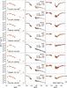 |
Fig. A.1 Left: SpeX spectra overlaid with 2MASS and WISE photometry. The identification of the sources in Table 1 and Fig. 1, and the 2MASS names are given at the bottom left. The SpeX spectra are scaled to Ks (2MASS) and W1 (WISE) band photometry, but by multiplying a single factor without adjusting K and L band spectra. Middle: zoom of the spectra from 2.0 to 3.9 μm. The best match template spectrum from IRTF spectral library is shown in orange in background. The excess absorption centered at 3.0 μm is attributed to the water ice. The best match spectral type, the visual extinction as measured by Román-Zúñiga et al. (2010, “CE” for color excess technique), and by matching the template stars (“SpeX”) are shown at the top right. Right: optical depth spectra at 3 μm. The optical depth spectrum calculated with the best matching template is shown in black, the second best in red, and the third best in orange to highlight the systematic uncertainty that stems from the choice of the templates. |
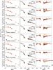 |
Fig. A.1 continued. |
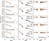 |
Fig. A.1 continued. |
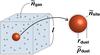 |
Fig. A.2 How the number of monolayers are translated to the column density of molecules. The first step is calculating the size of the cube (l) assigned to a single grain shown as a red ball in the picture. |
Appendix B: Translation of monolayers to column density
The simulations discussed in the paper, except Hocuk et al. (in prep.), do not provide the expected amount of ice column density that we can directly compare with the observations. Instead, they assume a surface of a single grain, and solve time-dependent chemistry with the physical conditions given locally, such as gas density, AV counted from the edge of the cloud, and dust temperature. The output is the number of layers of particular molecules in ice stacked on the grain surface. The simulations are not bound to any macroscopic setup, e.g., the size of the cloud. In order to compare the simulation with the observations, we need to translate the simulated ice molecular compositions on the grain surface to the column density of the ices through the cloud cores.
We start with a single spherical grain with the radius rdust = 0.1μm and calculate the size of the cube assigned to this particle that does not overlap with neighboring particles (Fig. A.2). The size of the box l is estimated, assuming a typical gas-to-mass ratio. The mass of a single grain particle is
![Mathematical equation: $$ {\tilde{M}_{\rm dust}} = \frac{4}{3} \pi r_{\rm dust}^3 ~\tilde{\rho}_{\rm dust} {\rm ~~~[g],} $$](/articles/aa/full_html/2018/02/aa29830-16/aa29830-16-eq120.png) where
where  is the mass density of the dust grain. The total number of gas-phase particles in the box, i.e., the number of mean mass molecules,
  amounts to
 ![Mathematical equation: \appendix \setcounter{section}{2} \begin{eqnarray*} \tilde{n}_{\rm gas} &=& \frac{\tilde{M}_{\rm gas}}{\mu_m m_H} \\[5mm] &=& \frac{\tilde{M}_{\rm dust}}{\mu_m m_H} \cdot \frac{\rho_{\rm gas}}{\rho_{\rm dust}}\\[5mm] &=& 4.5 \times 10^{11}, \end{eqnarray*}](/articles/aa/full_html/2018/02/aa29830-16/aa29830-16-eq123.png) where
where  is the total mass of the gas in the box, μm is the mean molecular weight 1.4, and mH is the mass of a hydrogen atom 1.67 × 10⁻²⁴ g. We used gas-to-dust mass ratio ρgas/ρdust ~ 100, and the mass density of the grain
  g cm-3. The typical transversal dimension of the cores in the Pipe Nebula, as measured by Román-Zúñiga et al. (2010), is ~0.1 pc in Shank and the peak visual extinctions through them are AV ~ 10 mag. The number densities of the gas in the cores are on the order of nH ≈ 104 cm-3. This is consistent with the positive detection of
C18O by Onishi et al. (1999) in these cores as well. The size of the cubic box is then ![Mathematical equation: \appendix \setcounter{section}{2} \begin{eqnarray*} l &=& \sqrt[\leftroot{-1}\uproot{2}\scriptstyle 3] {\frac{\tilde{n}_{\rm gas}}{n_{\rm H}}}\\ &=& 3.5 \times 10^2 {\rm ~~~[cm].} \end{eqnarray*}](/articles/aa/full_html/2018/02/aa29830-16/aa29830-16-eq132.png) On the other hand, the number of sites in one monolayer that molecules can stick to is
On the other hand, the number of sites in one monolayer that molecules can stick to is ![Mathematical equation: \appendix \setcounter{section}{2} \begin{eqnarray*} \tilde{n}_{\rm site} &=& 4 \pi r_{\rm dust} ^2/s^2 \\ &=& 1.4 \times 10^6 {\rm ~~~\left[molecule~mly^{-1}\right]}, \end{eqnarray*}](/articles/aa/full_html/2018/02/aa29830-16/aa29830-16-eq133.png) where s is the scale of the separation between the molecules on the surface, and therefore s2 is the area that one molecule holds. We assume that the grain surface is fully covered by a single layer of ice, and s = 3 Å. Scaling the result to a unit volume cm-3, the number density of the molecules when a grain is fully covered by a single layer of ice is
where s is the scale of the separation between the molecules on the surface, and therefore s2 is the area that one molecule holds. We assume that the grain surface is fully covered by a single layer of ice, and s = 3 Å. Scaling the result to a unit volume cm-3, the number density of the molecules when a grain is fully covered by a single layer of ice is ![Mathematical equation: \appendix \setcounter{section}{2} \begin{eqnarray*} n_{\rm site} &=& \tilde{n}_{\rm site} /l^3 \\ &=& 3.1 \times 10^{-2} {\rm ~~~\left[molecule~mly^{-1}\,cm^{-3}\right]}. \end{eqnarray*}](/articles/aa/full_html/2018/02/aa29830-16/aa29830-16-eq138.png) The translational dimension of the cores in the Pipe Nebula is again L ~ 0.1 pc or 3.1 × 1017 cm. Therefore, the monolayer of molecular ice in our particular case translates to a column density of
The translational dimension of the cores in the Pipe Nebula is again L ~ 0.1 pc or 3.1 × 1017 cm. Therefore, the monolayer of molecular ice in our particular case translates to a column density of ![Mathematical equation: \appendix \setcounter{section}{2} \begin{eqnarray*} N_{\rm mly} &=& n_{\rm site} \, L \\ &=& 9.6 \times 10^{15} {\rm ~~~\left[molecule~mly^{-1}\,cm^{-2}\right]}. \end{eqnarray*}](/articles/aa/full_html/2018/02/aa29830-16/aa29830-16-eq141.png)
All Tables
All Figures
|
Fig. 1 Extinction map of the Shank in the Pipe Nebula based on the near-infrared color excess (Román-Zúñiga et al. 2010). Overlaid are the positions of the targets. The sources where water ice is positively detected are marked by yellow crosses, while those with negative detections are marked by orange crosses. The zoom-in view of the positive detections at the regions A and B are shown in the middle and right panel, respectively. |
| In the text | |
|
Fig. 2 Optical depth spectra of water (3.0 μm; left column) and CO ice (4.672 μm; right column) toward the seven sources where water ice was positively detected in the observations by SpeX spectrograph at the IRTF. The numbering of the sources in Fig. 1 and Table 1 is shown at the bottom left of the water-ice panels with the 2MASS IDs. The CO ice spectra were obtained by NIRSPEC spectrograph at Keck II. The whole SpeX spectra including negative detections are compiled in Fig. A.1. Black, red, and orange plots, are the spectra in which photospheric features are removed by referring to the best, the second best, and the third best matching M-type template stars. The visual extinctions based on the color excess (AV CE; Román-Zúñiga et al. 2010) and on the template matching with the IRTF Spectral Library (AV SpeX; Rayner et al. 2009) are shown at the bottom right of the water ice spectra. |
| In the text | |
|
Fig. 3 CO ice spectra toward source #2 (17312818−2631268) recorded by NIRSPEC spectrograph. The black plot is the spectra binned by 21 pixels from the original sampling, and the gray plot by 11 pixels. The observed spectra shown in the three panels are identical. The laboratory spectra of CO ice obtained by Palumbo & Strazzulla (1993) are overlaid in red, dark orange, and light orange in each panel. The top panel shows the spectrum of CO ice deposited by itself, the middle panel CO ice deposited with CO2, and the bottom panel CO ice embedded in water ice. The dotted gray lines are the assumed continuum level with zero optical depths. The region marked in light gray indicates where the continuum level is uncertain. |
| In the text | |
|
Fig. 4 Comparison between AK from the near-infrared color excess (CE) technique by Román-Zúñiga et al. (2010) against the SpeX templates and the SED fitting. The boxes attached to AK measured by SpeX templates delineate the range of extinctions with 3 best matching templates. The dotted line represents the case where the AK’s would be identical to the color excess. |
| In the text | |
|
Fig. 5 Peak optical depth of the water ice (τ3.0) plotted against the visual extinction on the line of sight (AV). The three panels are all identical, but the area shown is smaller going from left to right. The enlarged areas are shown by dotted lines in the left panels. The canonical relation between τ3.0 and AV in Taurus found by Whittet et al. (2001) is shown by dashed lines. The measurements toward the Pipe Nebula are shown by filled yellow circles. Other measurements shown in the panels are from star-forming regions such as Taurus (Whittet et al. 1988; Smith et al. 1993; Murakawa et al. 2000), Lupus (Boogert et al. 2013), and IC 5146 (the Cocoon Nebula, Chiar et al. 2011). Two starless cores, L 183 (Whittet et al. 2013), L 429 (Boogert et al. 2011), and the globules in the Southern Coalsack (Smith et al. 2002) are shown as well. The linear regression fit to the data points from the Pipe Nebula is depicted by the gray line. Filled gray circles are the same as yellow circles, but after reducing AV by 25% from those in Román-Zúñiga et al. (2010). |
| In the text | |
|
Fig. 6 Column densities of CO (left) and CO2 (right) ices plotted against that of water ice. The measurements of CO ice toward the Pipe Nebula are all upper limits (yellow triangles) except for 17312818−2631268 (source # 2) shown in the yellow circle. The gray circle is the column density of CO ice on source #2 as well, but measured assuming that the short-wavelength shoulder 4.655–4.665 μm is part of the continuum (see Sect. 2.2.3). No observation of CO2 ice is available in the Pipe Nebula. Other measurements shown are from Taurus (Whittet et al. 2007), L 183 (Whittet et al. 2013), CK 2 (Knez et al. 2005), IC 5146 (Q21-1; Chiar et al. 2011), assorted quiescent clouds (Noble et al. 2013), Lupus (Boogert et al. 2013), and L 429 (Boogert et al. 2011). All the measurements are against the continua of background field stars through quiescent clouds. Only those lines of sight where both CO and CO2 ices are positively detected are shown. Four simulations of ice formation are compared with the observations (Hocuk et al. (in prep.); Vasyunin & Herbst 2013; Garrod & Pauly 2011; Pauly & Garrod 2016). The number of layers presented in the simulations are converted to the column density by assuming that one monolayer corresponds to 9.6 × 1015 cm-2 (Appendix B). Model column densities calculated with conversion factors that are two times larger and smaller are shown by the shaded areas. |
| In the text | |
|
Fig. A.1 Left: SpeX spectra overlaid with 2MASS and WISE photometry. The identification of the sources in Table 1 and Fig. 1, and the 2MASS names are given at the bottom left. The SpeX spectra are scaled to Ks (2MASS) and W1 (WISE) band photometry, but by multiplying a single factor without adjusting K and L band spectra. Middle: zoom of the spectra from 2.0 to 3.9 μm. The best match template spectrum from IRTF spectral library is shown in orange in background. The excess absorption centered at 3.0 μm is attributed to the water ice. The best match spectral type, the visual extinction as measured by Román-Zúñiga et al. (2010, “CE” for color excess technique), and by matching the template stars (“SpeX”) are shown at the top right. Right: optical depth spectra at 3 μm. The optical depth spectrum calculated with the best matching template is shown in black, the second best in red, and the third best in orange to highlight the systematic uncertainty that stems from the choice of the templates. |
| In the text | |
|
Fig. A.1 continued. |
| In the text | |
|
Fig. A.1 continued. |
| In the text | |
|
Fig. A.2 How the number of monolayers are translated to the column density of molecules. The first step is calculating the size of the cube (l) assigned to a single grain shown as a red ball in the picture. |
| In the text | |
Current usage metrics show cumulative count of Article Views (full-text article views including HTML views, PDF and ePub downloads, according to the available data) and Abstracts Views on Vision4Press platform.
Data correspond to usage on the plateform after 2015. The current usage metrics is available 48-96 hours after online publication and is updated daily on week days.
Initial download of the metrics may take a while.