Are cosmological gas accretion streams multiphase and turbulent?

Nicolas Cornuault; Matthew D. Lehnert; François Boulanger; Pierre Guillard

doi:10.1051/0004-6361/201629229

Home

All issues

Volume 610 (February 2018)

A&A, 610 (2018) A75

Full HTML

Free Access

Issue		A&A Volume 610, February 2018


Article Number		A75
Number of page(s)		14
Section		Extragalactic astronomy
DOI		https://doi.org/10.1051/0004-6361/201629229
Published online		05 March 2018

A&A 610, A75 (2018)

Are cosmological gas accretion streams multiphase and turbulent?

Nicolas Cornuault¹, Matthew D. Lehnert¹, François Boulanger²^,3 and Pierre Guillard¹

¹ Sorbonne Universités, UPMC Paris VI, CNRS UMR 7095, Institut d’Astrophysique de Paris, 98bis bd Arago, 75014 Paris, France
e-mail: cornuault@iap.fr; lehnert@iap.fr
² Institut d’Astrophysique Spatiale, CNRS UMR 8617, Université Paris-Sud 11, Bâtiment 121, Orsay, France
³ Research associate at the Institut d’Astrophysique de Paris, 98bis bd Arago, 75014 Paris, France

Received: 30 June 2016
Accepted: 20 October 2017

Abstract

Simulations of cosmological filamentary accretion reveal flows (“streams”) of warm gas, T ~ 10⁴ K, which bring gas into galaxies efficiently. We present a phenomenological scenario in which gas in such flows, if it is shocked as it enters the halo as we assume and depending on the post-shock temperature, stream radius, its relative overdensity, and other factors, becomes biphasic and turbulent. We consider a collimated stream of warm gas that flows into a halo from an overdense filament of the cosmic web. The post-shock streaming gas expands because it has a higher pressure than the ambient halo gas and fragments as it cools. The fragmented stream forms a two phase medium: a warm cloudy phase embedded in hot post-shock gas. We argue that the hot phase sustains the accretion shock. During fragmentation, a fraction of the initial kinetic energy of the infalling gas is converted into turbulence among and within the warm clouds. The thermodynamic evolution of the post-shock gas is largely determined by the relative timescales of several processes. These competing timescales characterize the cooling, expansion of the post-shock gas, amount of turbulence in the clouds, and dynamical time of the halo. We expect the gas to become multiphase when the gas cooling and dynamical times are of the same order of magnitude. In this framework, we show that this mainly occurs in the mass range, M_halo ~ 10¹¹ to 10¹³ M_⊙, where the bulk of stars have formed in galaxies. Because of the expansion of the stream and turbulence, gas accreting along cosmic web filaments may eventually lose coherence and mix with the ambient halo gas. Through both the phase separation and “disruption” of the stream, the accretion efficiency onto a galaxy in a halo dynamical time is lowered. Decollimating flows make the direct interaction between galaxy feedback and accretion streams more likely, thereby further reducing the overall accretion efficiency. As we discuss in this work, moderating the gas accretion efficiency through these mechanisms may help to alleviate a number of significant challenges in theoretical galaxy formation.

Key words: instabilities / galaxies: evolution / galaxies: halos / galaxies: formation / methods: analytical

© ESO 2018

1 Introduction

The realization that we live in a dark matter-dominated universe led to the development of the first comprehensive theory of galaxy formation (e.g., White & Rees 1978; Fall & Efstathiou 1980). These analytic models embedded simple gas physics into the hierarchical growth of structure whereby smaller halos merged over time forming successively more massive halos (White & Rees 1978). Despite the successes of this model in understanding the scale of observed galaxy masses, it was soon realized that there were a number of problems. The most significant of these problems is that modeled galaxies form with a higher fraction of baryons than is observed (e.g., Ferrara et al. 2005; Bouché et al. 2006; Anderson & Bregman 2010; Werk et al. 2014). This failure was dubbed the overcooling problem (Benson et al. 2003).

As numerical simulations allowed for galaxy growth to be coupled to the development of large-scale structure, these studies showed that much of the accreting mass may penetrate into the halo as filaments of gas and dark matter (Kereš et al. 2005; Ocvirk et al. 2008). Whether or not these streams pass through a stable accretion shock as they penetrate the halo depends on the mass and redshift of the halo (Birnboim & Dekel 2003; Dekel & Birnboim 2006, hereafter BD03 and DB06 respectively). If the shock is not stable, the accretion flow is “cold” (Dekel & Birnboim 2006).

This cold mode accretion in simulations occurs as streams of warm (10⁴ K) gas entering the halo are smoothed at kpc-scale and weakly coupled to the infalling dark matter filaments (Danovich et al. 2015; Wetzel & Nagai 2015). Cold mode accretion is efficient in reaching down to a few tenths of a virial radius (Dekel & Birnboim 2006; Behroozi et al. 2013). The high efficiency of gas accretion in some simulations leads to model galaxies with unrealistically high baryon fractions emphasizing the overcooling problem. To alleviate the problem of excess baryons in simulated galaxies, efficient outflows and feedback were introduced (e.g., Hopkins et al. 2012, 2016). Feedback both heats the gas in the halo, preventing it from cooling and also ejects gas from both the galaxy and halo, thereby lowering their total gas content.

The circumgalactic media of galaxies are certainly not devoid of gas, perhaps containing up to approximately half of the total baryon content of the halo (e.g., Werk et al. 2014; Peek et al. 2015). This gas is known empirically to be multiphase. The multiphase nature of halo gas is most evident in local high mass halos, those with masses on the scales of cluster or groups. In clusters, for example, even at constant pressure, a very wide range of gas phases are observed, from hot X-ray emitting gas to cold, dense molecular gas (e.g., Jaffe et al. 2005; Edge et al. 2010; Salomé et al. 2011; Tremblay et al. 2012; Hamer et al. 2016; Emonts et al. 2016). In galaxy halos, the detection of multiphase gas is mostly through the absorption lines from warm neutral and ionized gas (≲10⁴ to ~10⁶ K) and dust via the reddening of background galaxies and quasars (Ménard et al. 2010; Peek et al. 2015, but see Pinto et al. 2014 for the detection of hot gas in X-ray emission lines). Outflows from galaxies are also multiphase (e.g., Beirão et al. 2015; Heckman & Thompson 2017) and are likely crucial for creating and maintaining the multiphase gas in halos (e.g., Gaspari et al. 2012; Sharma et al. 2012b; Borthakur et al. 2013; Voit et al. 2015a; Hayes et al. 2016).

There is only circumstantial evidence for smooth, collimated accretion streams penetrating into galaxy halos (e.g., Martin et al. 2015; Bouché et al. 2016; Vernet et al. 2017, and references therein). In analogy with analyses of gas in halos and outflows, a phenomenological approach may provide additional insights into the nature of flows and halos that galaxy simulations are perhaps not yet achieving (e.g., Sharma et al. 2010, 2012b,a; Singh & Sharma 2015; Voit et al. 2015a,b; Thompson et al. 2016). The motivation to analyze gas accretion flows phenomenologically developed from the notion that overcooling remains a problem in simulations, there is scant observational evidence forthe streams of the type currently simulated, and high speed collisions of gas can lead to multiphase turbulent media (Guillard et al. 2009, 2010; Ogle et al. 2010; Peterson et al. 2012; Appleton et al. 2013; Alatalo et al. 2015).

Just as with the explanation for the lack of cooling flows in clusters (e.g., Peterson et al. 2003; Rafferty et al. 2008), our current understanding of accretion flows in galaxy halos may also suffer from an overly simplistic view of gas thermodynamics. In clusters, it is now understood that heating and cooling are in approximate global balance, preventing the gas from cooling catastrophically (e.g., Rafferty et al. 2008; Sharma et al. 2012b,a; McCourt et al. 2012; Zhuravleva et al. 2014; Voit et al. 2015b). In analogy with gas in cool core clusters, and in contrast to what a number of cosmological simulations currently show, the gas in streams may not cool globally.

Instead, if the gas in streams is inhomogeneous and subject to thermal and hydrodynamic instabilities (e.g., Sharma et al. 2010), the differences in cooling times between the gas phases leads to fragmentation of the gas. If streams are unstable, their gas will not remain monophasic or laminar. Thus, our goal in this paper is to investigate the question posed in the title: “Are cosmological gas accretion streams multiphase and turbulent?”. If yes, the gas energetics may regulate the gas accretion efficiency. Dekel et al. (2013) estimated the penetration efficiency over large halo scales at z ~ 2 of ~50% but this estimate only considered macroscopic processes that may influence the accretion efficiency. Because heating and cooling are controlled by the mass, energy, and momentum exchanges between the gas phases, a careful investigation of the gas physics on microscopic scales is required to determine whether or not microphysical gas processes may further reduce the efficiency of gas accretion onto galaxies.

To investigate the question posed in the title, we begin by presenting a qualitative sketch of our scenario, making a quantitative investigation of the impact of expansion in the post-shock gas on an accretion flow, discussing the case in which the post-shock gas has small fluctuations in density and temperature, and developing a criterion for when the gas fragments (Sect. 2). We also discuss the thermodynamic evolution of the streaming gas and how it becomes multiphased in Sects. 2.3 and 2.4. In Sect. 3, we discuss the consequences of the formation of a multiphase flow on the dynamical evolution of the stream after it penetrates the halo. To gauge the astrophysical pertinence of our model and to illustrate specific phenomena within the streaming gas, we analyze the physical characteristics of an idealized gas accretion stream penetrating a halo of 10¹³ M_⊙ at z = 2 throughout Sects. 2 and 3. In Sect. 4, we discuss why simulations may be missing some ingredients necessary for modeling accretion shocks robustly and outline a few simple consequences of our proposed scenario.

2 Our framework for multiphased streams

The idea that gas in halos is multiphase has been suggested for decades (e.g., Binney 1977; Maller & Bullock 2004). More recent studies of halo gas attribute the development of multiphase gas to the growth of local thermal instabilities (e.g., Sharma et al. 2010) or galaxy outflows (e.g., Thompson et al. 2016; Hayes et al. 2016). Gas instabilities are only relevant when the cooling time of the unstable gas is of the same order of magnitude or smaller than the dynamical time of the halo (e.g., Sharma et al. 2012b; McCourt et al. 2012). Ambient gas in halos and outflows from galaxies must often meet the necessary requirements for instability given that they are observed to be multiphase. However, in an accreting stream of gas, it is difficult to understand how the gas might achieve a balance between heating and cooling. We may have to consider other processes to determine if it is possible for streams themselves to become multiphased as they flow into the halo. In the following sections, we examine the physics of gas flowing into halos from cosmic web filaments.

2.1 Qualitative sketch of our specific framework

We briefly qualitatively outline our scenario of gas accretion through streams, sketched in Fig. 1, introducing the concepts developed later in the paper. We consider a collimated stream of warm gas with a temperature of 10⁴ K that penetrates into a dark matter halo filled with hot gas at the halo virial temperature. The density distribution of the hot gas smoothly follows the density distribution of the underlying dark matter halo. The ambient halo gas has a long cooling time and has constant density and temperature during the flow. The speed of the flow is set to the virial velocity of the halo and is highly supersonic relative to the sound speed of the gas within the stream. In the following we introduce the three basic physical ingredients of our modeling of streams.

As the stream penetrates at the virial radius, we assume it is shock heated whenever the hot halo gas provides the necessary pressure support for sustaining the shock (Sect. 2.2). The post-shock gas is overpressurized relative to the ambient halo gas and expands, invalidating the classical one-dimensional analysis of streams (DB06, Mo et al. 2010). The hot post-shock gas mixes with the ambient halo gas, which prevents much of the gas initially in the stream from cooling completely to form a monophasic post-shock stream. We further posit that the post-shock gas develops inhomogeneities due to, for example, non-planarity or obliqueness of the shock-front or through inhomogeneities in velocity and/or density of the stream before it is shocked. The fragmentation of the gas into hot and warm cloudy phases is central to our scenario. If certain physical conditions are met, theexpanding inhomogeneous gas cools and fragments, forming a two phase medium – a hot phase with an embedded warm cloudy phase (Sect. 2.2). Density and velocity inhomogeneities in the post-shock gas may be amplified through gas cooling, leading to the formation of a multiphased flow (see Sect. 2.3). The thermodynamic evolution of the hot and warm gas follow distinct paths in the density-temperature plane (Sect. 2.4).

We expect that part of the kinetic energy of the infalling gas is converted to turbulence within the warm clouds and random cloud-cloud motions (e.g., Hennebelle & Pérault 1999; Kritsuk & Norman 2002; Heigl et al. 2018). If the level of turbulence is high or if the clouds are formed while the gas is expanding, the warm clouds may spread beyond the initial boundary of the collimated inflowing stream (Fig. 1 and Sect. 3). If these conditions are met, the stream decollimates. The thermodynamic evolution of the post-shock gas in the stream is largely determined by the timescales of several relevant processes – gas cooling, expansion of the hot phase, dynamical time of the halo, and the stream disruption due to turbulent motions – which we quantify in the remainder of this and the next section.

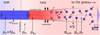Fig. 1

Sketch of our phenomenological picture of flows of gas passing through a virial shock. The initial inflowing gas (in blue) is overdense relative to the halo gas at the boundary by a factor f (=ρ₀ ∕ρ_H or the stream density divided by the density of the ambient halo gas at the virial radius), shocks at the boundary between the intergalactic medium (labeled “IGM”) and the hot halo gas (labeled “halo”). The persistent virial shock and the higher pressure of the post-shock gas compared to the ambient halo gas, allows the flow to expand after being shocked (labeled “expansion”). If certain conditions are met, the post-shock gas becomes unstable, fragmenting to form a biphasic medium. The fragmentation enables a fraction of the initial momentumand energy of the stream to be captured as turbulent clouds of warm gas with a dispersion, σ_turb, and a volume-filling factor, ϕ_v,w. If the level of turbulence is high enough, the clouds move beyond the initial radius of the stream, decollimating the flow. Eventually, the hot post-shock gas mixes with the ambient halo gas which prevents it from cooling further. See text and the Appendix for definitions of the variables.

2.2 Impact of expansion on the phenomenology of accretion flows

Since the pioneering work of White & Rees (1978) decades ago, the accretion of gas onto galaxies or into halos has been analyzed in one radial dimension, assuming homogeneity of the flow (see Mo et al. 2010). The one-dimensional approximation is also used for streams, where it is valid only if one can ignore lateral expansion. To determne whether this approximation is valid, one has to compare theexpansion to cooling time of the gas within the flow. Historically, even the analysis of the stability of the accretion shock neglected the possibility that the post-shock gas may expand into the ambient halo gas (DB06; Mo et al. 2010). In our study, we reconsidered the sustainability of the accretion shock that occurs as the infalling filament collides with the ambient halo gas. To conduct this analysis, we compared the cooling time of the post-shock gas to various other measures of its dynamical evolution. For simplicity, we only compared the cooling time to the expansion time of the post-shock gas into the surrounding ambient halo gas and the dynamical time of the halo. Intuitively, one can understand that if the cooling time is significantly shorter than either the expansion or dynamical times, the stream after the shock quickly cools down and maintain much of its integrity. Such a shock can be unstable and this is essentially the textbook situation that has been considered already (Mo et al. 2010). If the cooling time of the post-shock gas is significantly longer than either the expansion or dynamical times, then the post-shock gas mixes the ambient halo gas further supplying it with hot gas and entropy. This is another textbook example that has been analyzed one-dimensionally (DB06; Mo et al. 2010). However, if the cooling time is of the same order of magnitude of the expansion and halo dynamical times, a wider range of outcomes of the post-shock gas are possible (e.g., Sharma et al. 2010, 2012a). In this paper, we describe this more complex regime phenomenologically.

We now consider the impact of expansion on the properties of the post-shock gas. To estimate the cooling, expansion, and dynamical timescales, we introduce two parameters specific to the flow, its overdensity relative to that of mean density of gas at the virial radius, f, and the radius of the stream, r_stream. All variables used in this and subsequent sections are summarized in Tables A.1 and A.2. As we now show, the gas in the stream immediately after being heated to a high post-shock temperature, T_ps, has a pressure, P_ps, higher than the ambient halo gas, P_H, and thus expands into the surrounding ambient halo gas of density, ρ_H. All of the post-shock quantities are given by the normal Rankine-Hugoniot shock relations. The halo pressure at the virial radius is $P_{H} = (\frac{k_{B}}{μ m_{p}}) ρ_{H} T_{H} = \frac{(γ - 1)}{2} ρ_{H} v_{vir}^{2} = \frac{γ M_{1}^{2}}{3 f} P_{0},$ $\begin{equation*} P_{\mathrm{H}}=\left(\frac{k_{\mathrm{B}}}{\mu m_{\mathrm{p}}}\right)\rho_{\mathrm{H}} T_{\mathrm{H}}= \frac{(\gamma-1)}{2}\rho_{\mathrm{H}} v_{\mathrm{vir}}^2 =\frac{\gamma \mathcal{M}_1^2}{3f}P_0,\end{equation*}$ (1)

where T_H is the temperature of the ambient halo gas, which we assume to be the virial temperature. The pressure ratio just after the shock is $\frac{P_{ps}}{P_{H}} = \frac{2 f}{γ (γ + 1) \cdot g (M_{1})},$ $\begin{equation*} \frac{P_{\mathrm{ps}}}{P_{\mathrm{H}}}=\frac{2f}{\gamma \left(\gamma+1\right) \cdot g\left(\mathcal{M}_1\right)} ,\end{equation*}$ (2)

where $g : M_{1} \mapsto {(2 γ / (γ - 1) - M_{1}^{- 2})}^{- 1}$ $g:M_1\mapsto (2\gamma/(\gamma-1)-M_1^{-2})^{-1}$ . For γ = 5∕3 and within the domain [1, + ∞], this function rapidly decreases from 1:4 to 1:5. Hence the pressure ratio, P_ps ∕P_H is between 9:5 and 9:4 times the initial stream overdensity, f. Since f≳1, the pressureof the post-shock gas is higher than the pressure of the ambient halo gas. Thus, since the pressure ratio is always greater thanone, the flow expands into the halo gas.

To define the expansion time of the flow, we approximate this as the inverse of the relative rate of change of pressure in the post-shock gas as it expands. Quantitatively, this is written as $t_{expand} = P_{ps} / {\dot{P}}_{ps} = - 2 γ r_{stream} / {\dot{r}}_{stream} ~ 2 γ r_{stream} / c_{ps},$ $\begin{equation*} t_{\mathrm{expand}}=P_{\mathrm{ps}}/\dot{P}_{\mathrm{ps}}=-2\gamma r_{\mathrm{stream}}/\dot{r}_{\mathrm{stream}}\sim 2\gamma r_{\mathrm{stream}}/c_{\mathrm{ps}},\end{equation*}$ (3)

where r_stream is the radius of the stream before it expands and c_ps is the sound speed of the gas immediately after it has passed through the shock front. As a first-order approximation, for a homogeneous post-shock medium, one can easily compare the cooling and expansion times. Our definition of the expansion time means it is a differential measure of the expansion and so the most appropriate comparison is with the instantaneous cooling time of the gas immediately after the shock. The isobaric cooling time is defined as $t_{cool} (T) = T {| \frac{d T}{d t} |}_{P}^{- 1} = \frac{5 k_{B} ρ T}{2 μ n_{e} n_{H} Λ (T)} \approx 4.3 \times \frac{5 k_{B} μ m_{p} T}{2 ρ Λ (T)},$ $\begin{equation*} t_{\mathrm{cool}} (T) = T \left| \frac{\textrm{d}T}{\textrm{d}t} \right|^{-1}_P = \frac{5k_{\mathrm{B}} \rho T}{2 \mu n_{\textrm{e}} n_{\textrm{H}} \Lambda (T)} \approx 4.3 \times \frac{5k_{\mathrm{B}}\mu m_{\mathrm{p}} T}{2\rho\Lambda (T)},\end{equation*}$ (4)

where k_B is the Boltzmann constant, $Λ (T)$ $\Lambda\left(T\right)$ is the cooling efficiency as a function of temperature, T (Sutherland & Dopita 1993; Gnat & Sternberg 2007), μ is the mean molecular weight¹, m_p is the mass of the proton, ρ is the mass density of the cooling gas, n_e is the electron density, and n_H the hydrogen particle density². Hereafter, the cooling time of the post-shock is denoted by, t_cool,ps. We also refer to the cooling time after expansion as t_cool,pe.

The other timescale with which to compare the cooling time is the dynamical time of the halo. We estimate the dynamical time for matter falling from the virial radius with a radial velocity of v₂ (the post-shock velocity) directed at the center of the potential as $t_{ff} = α \frac{r_{vir}}{v_{2}} \approx t_{dyn, halo} .$ $\begin{equation*} t_{\mathrm{ff}}=\alpha \frac{r_{\mathrm{vir}}}{v_{2}}\approx t_{\mathrm{dyn, halo}}.\end{equation*}$ (5)

For this estimate, we assume a NFW dark matter potential (Navarro et al. 1997) and α = 1. α is a factor of order unity to account for the integrated gravitational acceleration during the fall. Assuming that the characteristic velocity and radius are the virial values, v_vir and r_vir, the dynamical time is independent of halo mass (Mo et al. 2010).

Figure 2 illustrates how these timescales depend on the post-shock temperature that are directly related to the halo mass (abscissa at the top) and for a range of relative stream overdensities, f, and relative stream radii, r_stream/r_vir, at z = 2. The initial stream penetrating the halo gas and the warm post-shock clouds are assumed to have a temperature of 10⁴ K, which is maintained through external heating processes, such as ionization by the meta-galactic flux or photons from the galaxy at the center of the halo potential. From this analysis, we see that the expansion times are almost constant above M_H ≳few 10¹⁰ M_⊙ since the virial shock is sufficiently strong such that t_expand ∝ t_dyn,halo. As f increases, the cooling times decrease systematically, which means for low temperatures (low mass halos at z = 2), the cooling time is always less than the expansion time. For very high mass halos, even for wide streams with relatively high densities, the cooling time is much longer than the expansion time and can be longer than the halo dynamical time for low to moderately overdense filaments. A wide range of values in f and r_stream/r_vir lead to cooling times that are less than the halo dynamical time and within an order of magnitude of the expansion time. Whenever the expansion time is comparable to the cooling time, the gas flow cools globally neither purely adiabatically or isobarically.

We can understand the competition between these timescales, t_cool,ps, t_cool,pe, t_dyn,halo, and t_expand, more clearly by considering them as a function ofthe stream overdensity, f, and post-shock temperature or halo mass (Fig. 3). For the case where t_cool,ps ≫ t_expand and t_cool,pe > t_dyn,halo, the post-shock gas expands rapidly remaining hot over at least a dynamical time of the halo. In this regime the hot post-shock gas likely mixes with the ambient halo gas, preventing significant cooling. This is akin the “hot mode accretion” discussed by Dekel and collaborators (e.g., DB06). In Fig. 3, we have labeled this regime, “hot accretion”. At the other extreme in Fig. 3, when t_cool,ps ≪ t_expand and t_cool,ps ≪ t_dyn,halo, the gas cools before there is significant expansion and before the stream has penetrated deeply into the halo. Accretion in this regime corresponds to their cold mode accretion and we labeled this as such in Fig. 3. Between these two regimes, t_cool,pe, t_cool,ps, t_dyn,halo, and t_expand are all about the same order of magnitude. In this regime, there is not a simple dichotomy between the types of accretion streams – they can be both hot and warm if the post-shock gas has a range of temperature and/or densities. Over this region, the thermodynamic evolution of the post-shock gas is more complicated. We labeled this regime “multiphase accretion”.

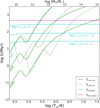Fig. 2

Timescale comparison of the competing relevant processes of cooling, expansion, and halo dynamics, for various post-shock temperatures (i.e., various halo masses), at z = 2. The solid green curves indicate the instantaneous post-shock cooling time, t_cool,ps, and the green dashed curves indicate the post-expansion cooling time, t_cool,pe – the cooling time of the post-shock gas after it has expanded sufficiently to reach pressure equilibrium with the ambient halo gas. The cooling time curves for the post-expansion gas are truncated at the minimum temperature, 10⁴ K, of the cooling efficiency used in our analysis (Gnat & Sternberg 2007). The cooling time curves were computed for three values of the initial overdensity f, as indicated by inclined green labels on the left side of the panel. Expansion times (solid cyan lines) are shown for three different relative filament radii, log r_stream /r_vir = −1, −1.5, and −2. The dynamical time, t_dyn,halo, which is independent of halo mass, is indicated by the horizontal magenta line.

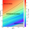Fig. 3

Ratio of the post-expansion cooling and halo dynamical timescales as a function of halo mass, M_H, and stream overdensity, f, at z = 2. The colors represent log (t_cool,pe∕t_dyn,halo) (Eqs. (4) and (5)) with corresponding values indicated in the color bar. Black contours indicate log (t_cool,pe∕t_dyn,halo) = 0 and 1 (solid) and log (t_cool,pe∕t_dyn,halo) = −1 (dashed). The white contours indicate values of log (t_cool,ps∕t_expand) (Eqs. (3) and (4)) equal to 0 and 1 (solid), and −1 (dashed). For this analysis, we assumed log (r_stream/r_vir) = −1.5. We highlight regions in which the cooling times are significantly longer than the halo dynamical times as hot accretion, regions in which the cooling time is significantly shorter than the dynamical times as cold accretion, and regions in which the cooling times are of the same order of magnitude as the dynamical times as multiphase accretion (see text for details). These labels are illustrative and are not intended to precisely delineate a separation of accretion modes. The gray region in the bottom right corner has T_pe < 10⁴ K, which is outside of the range of the cooling efficiency used in our analysis (Gnat & Sternberg 2007), and thus the values of log (t_cool,pe∕t_dyn,halo) are not defined.

2.3 Inhomogeneous infalling streams and post-shock gas: differential cooling

We now discuss the physical mechanisms behind the development of multiphasic accretion streams. Although our previous discussion of the relevant timescales considered homogeneous streams, density and velocity inhomogeneities may arise through the dynamics of the shock itself (Kornreich & Scalo 2000; Sutherland et al. 2003). Simulations show that stream are not accreted homogeneously but have substructure in both density and velocity (Nelson et al. 2016). Inhomogeneities may arise owing to a range of curvature in accretion shock fronts, translating into a range of Mach numbers and post-shock temperatures and densities. Density fluctuations at constant shock velocity also lead to inhomogeneities in the post-shock gas in both temperature and density resulting in a range of cooling times (Guillard et al. 2009). As we now discuss, once such “differential cooling” sets in, it acts like the thermal instability, leading to phase separation in the flow (Sharma et al. 2012b), but over a finite range of time in the absence of heating processes that balance the cooling of the hot phase.

To understand how the inhomogeneous post-shock gas evolves, we investigate how small fluctuations in the density and/or temperatureare amplified. Neglecting the influence of any heating process, the radiative cooling is not balanced and there are nofixed equilibrium points. Following closely the development presented in Sharma et al. (2012b), we begin with a parcel of gas that is overdense relative to an ambient medium. The magnitude of the overdensity is, δ ≡ |δρ∕ρ|~|δ T∕T| for isobaric conditions. The inverse of the effective cooling time of the overdense gas parcel relative to the ambient medium is, hence, $\frac{1}{t_{cool, eff}} = - \frac{1}{t_{cool, parcel}} + \frac{1}{t_{cool, ambient}} \cdot$ $\begin{equation*} \frac{1}{t_{\mathrm{cool, eff}}} = -\frac{1}{t_{\mathrm{cool, parcel}}} + \frac{1}{t_{\mathrm{cool, ambient}}}\cdot\end{equation*}$ (6)

As already shown by Sharma et al. (2012b), for small overdensities, δ ≤ 1, the inverse of the effective cooling time under isobaric conditions is written as $\frac{1}{t_{cool, eff}} ~ - δ \frac{\partial}{\partial \ln T} {(\frac{1}{t_{cool}})}_{P} = \frac{δ}{t_{cool}} [2 - \frac{d \ln Λ (T)}{d \ln T}] \cdot$ $\begin{equation*} \frac{1}{t_{\mathrm{cool, eff}}} \sim -\delta \frac{\partial}{\partial{\,\ln T}} \Bigg(\frac{1}{t_{\mathrm{cool}}} \Bigg)_{\mathrm{P}} = \frac{\delta}{t_{\mathrm{cool}}} \Bigg[2 - \frac{\diff\ln\Lambda(T)}{\diff\ln T} \Bigg]\cdot\end{equation*}$ (7)

Marginally denser gas cools faster than the gas in which it is embedded and the cooling becomes a runaway process for temperatures ≳10⁵ K and around few 10⁴ K at low metallicities (right panel in Fig. 6). We refer to this process as “differential cooling". As soon as heterogeneities form in approximate pressure equilibrium with their surroundings, denser cooler regions of the gas cool rapidly and form clouds, leaving a high volume-filling inter-cloud medium that is hotter and rarer than the clouds. Thus, differential cooling leads to multiphasic post-shock accretion flows. This is akin to what occurs for thermally unstable gas (Field 1965) but the phase separation is transient in the absence of heating processes of the hot gas to balance its cooling.

Of course, a natural consequence of differential cooling is that even for halo masses where the post-shock gas has on average a long cooling time, gas with fluctuations in temperature or density may locally cool sufficiently rapidly to form a multiphased medium.

Analytically, inhomogeneities can be accounted for as is done in phenomenological analyses of the formation of stars through the use of probability distribution functions (PDFs) in gas density and/or temperature (e.g., Hennebelle & Chabrier 2009). We follow the thermodynamical evolution of the temperature and density PDFs using the energy equation, namely, $\dot{e} = - ρ \frac{Λ (T)}{4.3 μ m_{p}} + P \frac{\dot{ρ}}{ρ^{2}},$ $\begin{equation*} \dot{e} = -\rho \frac{\Lambda(T)}{4.3 \mu m_{\textrm{p}}} + P\,\frac{\dot{\rho}}{\rho^2},\end{equation*}$ (8)

where e is the specific internal energy. We illustrate the isobaric evolution of inhomogeneities in a flow using such an approach in Fig. 4. In this illustration, we consider a lognormal PDF in temperature with a dispersion of σ_T = 0.3 (1σ dispersion in $\log \frac{ρ}{ρ_{ps}} = \log \frac{T}{T_{ps}}$ $\log \frac{\rho}{\rho_{\mathrm{ps}}} = \log \frac{T}{T_{\mathrm{ps}}}$ ). We chose a gas pressure and mean temperature appropriate for the post-shock gas of a flow into a massive, 10¹³ M_⊙, halo at z = 2. For this illustration, the gas pressure is P_ps /k_B = 5.8 × 10⁴ K cm⁻³ and the initial post-shock temperature T_ps = 2.7 × 10⁶ K. We find that a substantial fraction of the accreting gas cools to 10⁴ K in a fraction of t_cool,ps, while the peak of the hot gas temperature PDF does not shift with time (Fig. 4).

We show in Fig. 5 both the mass fraction and volume-filling factor of the gas for the warm, 10⁴ K gas as a function of time. We calculated the mass fraction by integrating the amount of gas that cools to 10⁴ K as a function of time, $ϕ_{m, w} = \int_{0}^{10^{5} K} \frac{d m}{d T} d T / \int_{0}^{T_{max}} \frac{d m}{d T} d T,$ $\begin{equation*} \phi_{\mathrm{m,w}} = \int_{0}^{10^5 K} \frac{\textrm{d}m}{\textrm{d}T} \, \textrm{d}T / \int_0^{T_{\mathrm{max}}} \frac{\textrm{d}m}{\textrm{d}T} \, \textrm{d}T,\end{equation*}$ (9)

where dm is the gass mass between T and T + dT. The volume-filling factor was calculated using, $ϕ_{v, w} = \int_{0}^{10^{5} K} \frac{1}{ρ} \frac{d m}{d T} d T / \int_{0}^{T_{max}} \frac{1}{ρ} \frac{d m}{d T} d T .$ $\begin{equation*} \phi_{\mathrm{v,w}} = \int_{0}^{10^5 K} \frac{1}{\rho}\, \frac{\textrm{d}m}{\textrm{d}T} \, \textrm{d}T / \int_0^{T_{\mathrm{max}}} \frac{1}{\rho}\, \frac{\textrm{d}m}{\textrm{d}T} \, \textrm{d}T.\end{equation*}$ (10)

We note that the results shown on Figs. 4 and 5 are plotted as a function of the post-shock cooling time t_cool,ps. The timescale normalized in this way is, to first order, independent of the specific values of ρ_ps and T_ps. These results even apply to the gas cooling after expansion when t_expand < t_cool,ps. Figure 5 shows that the warm gas becomes the dominant mass phase, within about half of the post-shock cooling time, and that the warm gas only fills a small fraction of the volume. For a higher value of the temperature dispersion σ_T, ϕ_m,w increases over a broader range of fractional times distributed around the same time required for half the mass to cooling in our specific illustration.

In Fig. 5, the gas is multiphase for only a few t_cool,ps. The hot gas eventually cools because we have not considered any heating processes. However, the process of fragmentation of the gas could be sustained if there is heating of the hot gas. Even in absence of heating, after expansion the hot gas eventually mixes with the ambient halo gas thus sustaining the hot phase. Possible local sources of heating for the post-shock gas are the radiative precursor of high velocity shocks, thermal conduction, radiation from the surrounding hot medium, cloud-cloud collisions, and dissipation of turbulence. The mechanical energy input from active galactic nuclei (AGN), winds generated by intense star formation, and other processes can plausibly balance the cooling of the hot gas globally (e.g., Best et al. 2007; Rafferty et al. 2008). Overall, there is more than enough energy, but what is unknown is how and with what efficiency this energy is transferred to the streaming gas. Even though simulations do not capture this process, it has been suggested that the energy from the galaxy is transferred efficiently through turbulent energy cascade and dissipation (Zhuravleva et al. 2014; Banerjee & Sharma 2014).

We ask the poignant question whether the flowing post-shock gas can actually become multiphase while cooling in a halo dynamical time. It is a difficult question to answer in the particular case of accretion streams because it depends on how inhomogeneous the gas is. It occurs if the post-shock conditions are sufficiently inhomogeneous. The gas becomes multiphased around when t_cool,pe is the same order of magnitude as t_dyn,halo. This justifies where we placed the “multiphase accretion” label in Fig. 3. This figure shows that this occurs in the important mass range of M_halo ~ 10¹¹ to 10¹³ M_⊙ at z = 2. The values of course depend on the relative overdensity of the streams (f) and, through the characteristics of the halos, on redshift. The bulk of stars have formed in galaxies in halos within this mass range and z ≈ 2 is the epoch in which the peak of the comoving density of star formation occurs (Madau & Dickinson 2014, and references therein). Moreover, because the volume filling-factor of the warm gas is likely to always be small, even in the cases where the mass fraction is large, multiphase streams are likely to be difficult to identify observationally using QSO absorption lines. We discuss this further in Sect. 4.

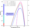Fig. 4

Temperature probability distribution function, dP/dln T, as a function of the gas temperature at various times during isobaric cooling. The initial distribution (magenta line) is lognormal with a dispersion, σ_T = 0.3, initial mean gas temperature, T_ps = 2.7 × 10⁶ K, and initial pressure, P_ps/k_B = 5.8 × 10⁴ K cm⁻³. We show the distributions of gas temperature at 4 different times relative to t_cool,ps as indicated in the legend. In the last column of the legend, we provide the fraction of the gas that has cooled to 10⁴ K, f_M, at each fraction of the post-shock cooling time. For example, in this illustration, after one post-shock cooling time, even though the peak gas temperature of the PDF has changed very little, ≈85% of the gas has cooled to 10⁴ K. We represent these fractions in the colored bar in which each color corresponds to the PDF of the same color (the fractions, f_M are relative to the ordinate on the right side of the panel). Once the gas starts to cool differentially, it does so very rapidly, in less than t_cool,ps (large blue arrow).

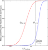Fig. 5

Change in the mass fraction, ϕ_m,w, and the volume filling-factor, ϕ_v,w, of the warm, 10⁴ K gas as a function of the post-shock cooling time (Eqs. (9) and (10)). The timescale is expressed in units of the isobaric cooling time, t_cool,ps, as defined inthe text. The initial values of the pressure and temperature are the same as those used in Fig. 4. We indicate the ratio of the halo dynamical and post-shock cooling times as a vertical black dotted line. This suggests that with our initial conditions, the stream has sufficient time to fragment significantly, but not reach a high volume-filling factor of warm gas. This suggests that even highly fragmented streams with high ϕ_m,w are challenging to identify and study via QSO absorption lines.

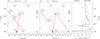Fig. 6

Left and middle: sketch of the thermodynamic path for cases (1) and (2) (see text). Σ₁ (red triangle) indicates the density and temperature of the pre-shock gas. The gas is shocked reaching the point Σ_ps. Subsequently, the gas cools adiabatically due to the expansion of the stream until the halo pressure is reached at Σ_h. Two phases separate. For case (1), phase separation occurs at Σ_h, while for case (2), it occurs at Σ_ps. In both cases, the hot component mixes with the surrounding halo gas, reaching Σ_H. For case (1), the warm component cools radiatively and isobarically to the point Σ_w. For case (2), the same point is reached but the gas takes a different thermodynamic path. Dashed black lines represent adiabats and isobars labeled A and I, respectively. The two blue-dashed curves in the left panel indicate contours of constant cooling time, t_cool ~ 0.2t_dyn,halo (upper curve) and t_cool ~ 0.12t_dyn,halo (lower curve). These curves indicate that the cooling time during the expansion remains approximately constant. (right) Analysis of the isobaric differential cooling “instability” (Eq. (8)) of low-, 10⁻³ solar (solid line) and solar-metallicity (dashed line) gas as a function of temperature. When 2 − d lnΛ∕ dlnT > 0 the gas can become heterogeneous through differential cooling if δ is sufficiently large. The post-shock temperature of our illustration lies within the region where the stream can become unstable.

2.4 Thermodynamic evolution of streams: why are some streams cloudy?

There are two limiting cases to consider specifically when attempting to understand the thermodynamic development of a biphasic stream. The two cases are (1) t_expand ≪ t_cool,ps and (2) t_expand ≫ t_cool,ps. In case (1); the warm phase develops only after the expansion has occurred, while in case (2) the clouds form before the expansion. We sketch the thermodynamic evolution (“paths”) of a stream in Fig. 6. To make these illustrations, we adopted f = 30 and r_stream/r_vir = 0.01 for case (1); and f = 150 and r_stream/r_vir = 0.1 for case (2) for a halo with a mass of 10¹³ M_⊙ at z = 2. For a halo of this mass, the post-shock gas temperature is such that, if the stream has a sufficiently high δ, it becomes unstable and fragments into warm and hot phases (right panel in Fig. 6).

In case (1), clouds fill the entire expanse of the expanded flow. Adiabatic expansion occurs before radiative cooling becomes important, the stream cools and the density of the hot phase declines without a change in entropy. In case (2), the two phases separate before expansion. In both cases, the hot post-shock gas reaches pressure equilibrium and mixes with the ambient halo gas.

These two conditions are of course for the limiting (simplest) cases, in reality, the gas has t_expand within an order of magnitude of t_cool,ps (Fig. 3). For these “intermediate” cases, the thermodynamic evolution is more complex, but, with our assumption that the hot gas cools adiabatically during expansion and the warm gas evolves isobarically, the clouds reach the same final thermodynamical state as illustrated in the two limiting cases. However, the gas in these intermediate cases does not necessarily end up with the same distribution of volume-filling factors and mass fractions.

The cooling length at the post-shock temperature is the size over which structures can cool isobarically (i.e., cooling length, λ_cooling,ps = c_ps t_cool,ps). In case (1), the cooling length is much larger than the stream radius, λ_cooling,ps ≫ r_stream, clouds may form over all scales within the stream. In case (2), it is much smaller, λ_cooling,ps ≪ r_stream, and clouds may form over a range of sizes smaller than the stream radius. The expansion of the hot gas does not inhibit the growth of thermal anddifferential cooling instabilities because the decrease in the pressure is roughly compensated by the decrease of temperaturealong an adiabat in the expression of the cooling time. In other words, for the post-shock temperature, i.e., for the halo mass we adopted, the gas cooling time remains roughly constant as the gas expands (Fig. 6; see also Fig. 2). Eventually, the warm phase equilibrates at approximately the halo pressure and the hot phase mixes with the halo gas. We are obviously considering fragmentation on scales much smaller than the scale height of the gravitational potential well and thus we can safely ignore thermal stabilization by convection (Balbus & Soker 1989; Sharma et al. 2010).

The thermodynamic paths we sketched in Fig. 6 exhibit phenomena that are generic to the evolution of fragmenting streams. We only use the initial conditions of the stream to illustrate the quantitatively the evolution of the gas (i.e., the temperatures and densities and their evolution). Streams fragment for a wide range of initial conditions and have a generally similar, but more complex, thermodynamic evolution.

3 Consequences of the formation of multiphased, cloudy accretion flows

3.1 Turbulence in warm clouds

As the gas fragments, perhaps due to differential cooling and/or thermal instabilities, we assume that some of the initial kinetic energy of the stream is converted into turbulence within the warm component. We parameterize the turbulence after phase separation as the ratio, η, of the turbulent energy density of the clouds and the initial bulk kinetic energy density of the stream. We define this ratio as $η = \frac{{< ρ_{w} >}_{v} σ_{turb}^{2}}{ρ_{1} v_{1}^{2}},$ $\begin{equation*} \eta=\frac{\langle\rho_{\mathrm{w}}\rangle_{\mathrm{v}} \sigma_{\mathrm{turb}}^2}{\rho_{\mathrm{1}} v_{\mathrm{1}}^2},\end{equation*}$ (11)

where ${< ρ_{w} >}_{v}$ $\langle\rho_{\mathrm{w}}\rangle_{\mathrm{v}}$ is the volume-averaged density of the warm clouds ( ${< ρ_{w} >}_{v} = ϕ_{v, w}$ $\langle\rho_{\mathrm{w}}\rangle_{\mathrm{v}}=\phi_{\mathrm{v,w}}$ ρ_w, where ϕ_v,w is volume-filling factor and ρ_w is the density of the warm clouds, respectively), σ_turb is the cloud-cloud velocity dispersion, ρ₁ and v₁ are the pre-shock gas density and velocity. We assume that v₁ is equal to the virial velocity, v_vir. The initial density of the stream is related to the hot halo density, ρ_H, as ρ₁ = fρ_H. The amount of turbulence generated in the post-shock gas is likely determined by as yet poorly understood and undoubtedly complex gas physics. In our model we do not attempt to investigate the complexity involved in this transformation of energy, we simply parameterize the amount of turbulence by η which is free.

As we briefly alluded to in Sect. 2.3, as the turbulent energy dissipates, it reheats the warm clouds, thereby moderating the cooling. The cooling of the clouds is also moderated by mixing with the ambient halo gas as the stream penetrates deeper into the halo potential (Fragile et al. 2004). Dissipation of turbulent kinetic energy in the hot phase may also contribute to heating the post-shock gas and the radiation from the high-speed accretion shock (Allen et al. 2008). The parameter η may be high enough to provide the required heating of the hot gas in the stream through turbulent dissipation and mixing with the halo gas, perhaps instigating thermal instabilities. On the other hand, η must be lowenough such that turbulent dissipation and mixing does not prevent instabilities, both thermal and cooling, from growing in the post-shock gas (Banerjee & Sharma 2014; Zhuravleva et al. 2014). These constraints and considerations may ultimately provide limits on how much or how little turbulence is sustainable in the post-shock gas, but determining these exact values requires further detailed study and is not considered here.

3.2 Mass and momentum budget of the multiphase medium

We assume that as the stream flows into the halo, its mass flow rate is conserved during the post-shock expansion and does not mix immediately with the ambient halo gas. This leads to the relation $S ρ_{2} v_{2} = ρ_{1} v_{1},$ $\begin{equation*} S\rho_2 v_2=\rho_{\mathrm{1}} v_{\mathrm{1}},\end{equation*}$ (12)

where ρ₂ is the density after the hot gas has expanded by a factor, S, and similarly, v₂ is its velocity (Fig. 1). The expansion factor, S, is defined as the ratio of the initial over the final mass fluxes (per unit surface perpendicular to the flow). The post-shock gas ultimately reaches pressure equilibrium with the halo, which implies ρ_w T_w = ρ_hT_h = ρ_HT_H, where ρ_w and ρ_h are the densities of the warm and hot components and T_H is the temperature of the hot components after phase separation in the post-shock gas.

Before there is any momentum exchange with the halo gas, the momentum of the streaming gas is conserved, implying $S (ρ_{2} v_{2}^{2} + η ρ_{1} v_{1}^{2} + P_{H}) = ρ_{1} v_{1}^{2} + P_{1},$ $\begin{equation*} S\left(\rho_2 v_2^2 + \eta\rho_1 v_1^2 + P_{\mathrm{H}}\right)=\rho_1 v_1^2 + P_1,\end{equation*}$ (13)

where P₁ is the initial pressure of the stream. We assume the fragmenting gas radiates away its heat until reaching a floor temperature, T_w = 10⁴ K. The hot component only cools adiabatically and reversibly (no heat transfer and no entropy increase) expanding after it passed through the shock front, namely, $ρ_{h}^{γ} P_{ps} = ρ_{ps}^{γ} P_{H}$ $\rho_{\mathrm{h}}^{\gamma} P_{\mathrm{ps}}=\rho_{\mathrm{ps}}^{\gamma} P_{\mathrm{H}}$ , where γ is the ratio of specific heats. This approximation holds until the expanding gas reaches pressure equilibrium with the ambient halo gas.

The expansion factor, S, is derived from Eqs. (1), (12), and (13), as $S = \frac{1}{2} {(η + \frac{γ - 1}{2 f})}^{- 1} (1 - \sqrt{1 - 4 \frac{ρ_{H}}{ρ_{2}} (η f + \frac{γ - 1}{2})}) \cdot$ $\begin{equation*} S=\frac{1}{2}\left(\eta+\frac{\gamma-1}{2f}\right)^{-1} \left(1-\sqrt{1-4\frac{\rho_{\mathrm{H}}}{\rho_{2}} \left(\eta f+\frac{\gamma-1}{2}\right)}\right)\cdot\end{equation*}$ (14)

The expansion of the stream is important in our formulation. It leads to the mixing of the expanding post-shock gas with the ambient halo gas. This mixing couples the hot post-shock gas to the larger energy reservoir of the ambient halo gas, which acts as a thermostat preventing the gas from cooling, thereby possibly maintaining the pressure necessary to support a sustained shock. As we discussed in Sect. 2, it is the relative ratios of the thermal cooling time and expansion time that influences how the stream evolves.

3.3 Disruption of cloudy streams

The relative cloud-cloud motions may lead to warm clouds spreading beyond the initial radius of the stream. So instead of the streams being highly collimated as we assumed they are initially (before the virial shock), the flows may decollimate. This can be thought of as disruption since the warm clouds expand away from the original trajectory of the stream, thus “disrupting” the flow. We define the timescale for disruption as the cloud crossing time of the stream, namely, $t_{disrupt} = \frac{r_{stream}}{σ_{turb}},$ $\begin{equation*} t_{\mathrm{disrupt}}=\frac{r_{\mathrm{stream}}}{\sigma_{\mathrm{turb}}},\end{equation*}$ (15)

where σ_turb may be computed from η, f, and the volume-filling factor of the warm clouds, ϕ_v,w. From Eqs. (1) and (11), assuming pressure equilibrium between gas phases, yields $\begin{array}{l} σ_{turb}^{2} & = & v_{1}^{2} (η f / ϕ_{v, w}) (T_{w} / T_{H}) \\ = & \frac{2}{(γ - 1)} (\frac{k_{B}}{μ m_{p}}) (η f / ϕ_{v, w}) T_{w} . \end{array}$ $\begin{equation*} \begin{aligned} \sigma_{\mathrm{turb}}^2&= v_{\mathrm{1}}^2 (\eta f/\phi_{\mathrm{v,w}}) (T_{\mathrm{w}}/T_{\mathrm{H}}) \\ &= \frac{2}{(\gamma-1)}\left(\frac{k_{\mathrm{B}}}{\mu m_{\textrm{p}}}\right)(\eta f/\phi_{\mathrm{v,w}}) T_{\mathrm{w}} \end{aligned}.\end{equation*}$ (16)

Characterized this way, $σ_{turb}^{2} / v_{1}^{2} > η$ $\sigma_{\mathrm{turb}}^2/v_{\mathrm{1}}^2>\eta$ . For a wide range of relative amounts of turbulent energy, stream overdensity, and volume-filling factor of the warm gas, the cloud-cloud dispersion be up to v_vir/2. The dynamical evolution of the stream is determined by the ratio of the disruption and halo dynamical time. If t_disrupt ≫ t_dyn,halo, then the warm clouds within the stream remain collimated as they flow, otherwise, the streams decollimates.

This is the only process we consider in determining whether or not the warm clouds travel coherently toward the galaxy proper as observed in numerical simulations (e.g., Brooks et al. 2009; Danovich et al. 2015). To illustrate this concept, we estimate t_disrupt/t_dyn,halo as functions of f and ϕ_v,w for a halo with a mass of 10¹³ M_⊙ at z = 2. (Figs. 7 and 8; Eqs. (5) and (15)). We find that the disruption time is shorter than or approximately equal to the halo dynamical time for this halo mass, redshift, and our assumed r_stream. Thus it appears that for a wide range of relative turbulent energy densities, stream overdensities, and volume-filling factors of the warm gas, the flows do not simply fall directly into the potential as a highly collimated, coherent streams. In reality, the clouds are dynamical entities, we expect clouds to keep forming through cooling as other clouds are destroyed by hydrodynamic instabilities and heated by dissipation (Cooper et al. 2009).

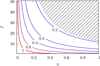Fig. 7

Disruption of the flow as a function of the filament overdensity, f, and level of turbulence, η. The contours represent constant ratios of t_disrupt∕t_dyn,halo as labeled (cf. Eqs. (5) and (15)). We assume a volume-filling factor of 0.1 (see Fig. 5) for the warm clouds and r_stream = r_vir/10. In regions with values less than 1, the streams are “disrupted” (Sect. 3.3). The shaded region indicates regions that are forbidden because for these values of the parameters, the post-shock pressure is less than the halo pressure. We note that because $t_{disrupt} \propto σ_{turb}^{- 1}$ $t_{\mathrm{disrupt}}\propto \sigma_{\mathrm{turb}}^{-1}$ , the contours of constant t_disrupt∕t_dyn,halo are shaped like contours of constant σ_turb in the same plane. For example, the contour, t_disrupt∕t_dyn,halo = 0.2, is close to the contour for σ_turb = 200 km s⁻¹, which is almost half the initial velocity of the flow.

4 Discussion

We now discuss broadly how our findings relate to several aspects of galaxy formation and evolution.

4.1 Are virial shocks persistent?

In our scenario, the existence of a hot phase in hydrostatic equilibrium supports a persistent shock (Binney 1977; Maller & Bullock 2004). Cosmological simulations appear to show a similar phenomenology as that described in DB06. Depending on the mass of the halo and redshift, streams penetrate at about one to many 100s of km s^-1 (van de Voort & Schaye 2012; Goerdt & Ceverino 2015) or much greater than the sound speed of the stream, c_s ~ 10–20 km s^-1. Simulated accretion shocks are “isothermal” at high Mach numbers and not stable (e.g., Nelson et al. 2016, 2015). Perhaps this uniform isothermality is due to the spatial and temporal resolutions adopted in the cosmological simulations. The scales that simulations must probe are roughly delineated in one-dimensional shock calculations. Raymond (1979) showed that atomic shocks with velocities of ~100 km s^-1 reach their post-shock temperatures within a distance of ≈1–10 × 10¹⁵ cm in less than ~30 yr. For higher shock velocities, the spatial and temporal scales are even shorter (Allen et al. 2008). The gas cools after the shock on timescales that are at most only a couple of orders of magnitude longer. In addition, to capture the differential cooling and thermal instabilities in the post-shock gas, resolutions much finer than the Field length are required (Koyama & Inutsuka 2004; Gressel 2009). Simulations should be specifically designed to capture the multiphase nature of streams penetrating halos to test our scenario by resolving the Field length (Koyama & Inutsuka 2004). Since the Field length decreases strongly with decreasing temperature, this is most easily done with ad hoc floor temperature higher than 10⁴ K but lower than the virial temperature as done for simulating thermal instabilities in cool core clusters (McCourt et al. 2012).

The resolution and temporal scales necessary to resolve high Mach number shocks are not achievable in galaxy- or cosmological-scale simulations. To overcome this limitation, numericists have taken advantage of numerical viscosity or use artificial viscosity in the form of a dissipative term either in dynamical equations or dispersion relations, depending on the properties of the gas or the flow (e.g., Kritsuk et al. 2011; Price 2012; Hu et al. 2014; Beck et al. 2016). Viscosity spreads the shock over several resolution elements, thereby enabling simulations to resolve heating and cooling across the shock front. The Reynolds number is inversely proportional to the kinetic viscosity of the fluid. If the flow properties were unchanged but the viscosity increased, the Reynolds number of the flow would be artificially low. Simulations with artificial or numerical viscosity have flows with low Reynolds numbers. Simulated low Re flows, Re ≲1000, tend to be laminar. Those with low spatial and temporal resolutions due to not resolving the Field length and having unrealistically low Reynolds numbers likely fail to produce biphasic turbulent flows (see, e.g., Kritsuk & Norman 2002; Sutherland et al. 2003; Koyama & Inutsuka 2004; Kritsuk et al. 2011; Nelson et al. 2016, for discussion).

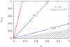Fig. 8

Disruption of the flow as a function of the volume-filling factor of the warm gas and level of turbulence. The contours represent constant ratios of t_disrupt /t_dyn,halo as labeled (cf. Eqs. (5) and (15)). We assume f = 30 and r_stream = r_vir/10. In regions with values less than 1, the streams are disrupted. The shaded region has the same meaning as in Fig. 7.

4.2 Nature of flows into galaxies: observational tests

As a consequence of our assumption that all energetic quantities scale as v_vir, the cloud-cloud dispersion is a simple linear function of η, f, and $ϕ_{v, w}^{- 1}$ $\phi_{\mathrm{v,w}}^{-1}$ . This relation implies that turbulent velocities of the warm clouds in the post-shock gas are independent of both halo mass and redshift. In principle this means that post-shock streams may be turbulent in any halo at any redshift. The reality is probably much more complex, through both macro- and microscopic gas physics, which is not yet understood well, the two parameters, η and ϕ_v,w, likely depend on the accretion velocity and the physical state of the ambient halo gas – both of which undoubtedly depend on redshift and halo mass.

Our scenario has observationally identifiable consequences. If our scenario is realistic, then observations should reveal: clumpy, turbulent streams and strong signs of the dissipation of turbulent mechanical energy in the warm medium (e.g., Guillard et al. 2009; Ogle et al. 2010; Tumlinson et al. 2011). The situation described in our model, namely, that a large fraction of the bulk kinetic energy of the accretion flow is transfered to turbulent motions among cold clouds, is observed in large-scale galaxy colliding flows, such as the situation in the Taffy Galaxies or Stephan’s Quintet, where we see evidence for this energy cascade (Peterson et al. 2012; Cluver et al. 2010). In Stephan’s Quintet, two atomic gas filaments are colliding at ~1000 km s^-1 and yet instead of finding intense X-ray emission from the post-shock gas, most of the kinetic energy is contained in the turbulent energy of the warm molecular gas (Guillard et al. 2009, 2010). Remarkably, roughly 90% of the bulk kinetic energy has not been dissipated in the large-scale shock and is available to drive turbulence. If gas in colliding flows is multiphase and turbulent, then it may be the case as well for accretion streams.

Obviously, a clumpy stream is difficult to identify as such through absorption line spectroscopy, which may explain why streams have not been conspicuously identified so far. This is most obviously seen in Fig. 5, where even though a large fraction of the gas is warm, its volume-filling factor is, for a significant fraction of the dynamical time, minuscule. Along most lines of sight, absorption-line spectroscopy is expected to sample only the hot, high volume-filling factor halo gas or probe a population of warm ambient halo clouds (Maller & Bullock 2004; Tumlinson et al. 2011; Werk et al. 2014). The clouds should be looked for in emission, a process that depends on the square of the density, since the density increases during differential cooling, the emission is enhanced. Their emission can be powered by the meta-galactic flux, UV radiation from the central galaxy of the halo, and loss of their gravitational potential energy as they fall into the halo. These processes have already been modeled in simulations (e.g., Goerdt et al. 2010; Rosdahl & Blaizot 2012; Cen & Zheng 2013). In our scenario, streams can be additionally powered by the localized dissipation of turbulent energy, shock heating through cloud-cloud collisions, and radiation from the shock front. This may have already been observed in Lyα (e.g., Cantalupo et al. 2014; Martin et al. 2015). In particular, it would be promising to interpret spectral-imaging observations such as those provided by MUSE on the ESO/VLT within the context of our scenario (see Borisova et al. 2016; Fumagalli et al. 2016; Vernet et al. 2017).

4.3 Moderating the accretion rate: Biphasic streams and increased coupling between “feedback” and accretion

In our phenomenological model, two mechanisms moderate the accretion efficiency on to galaxies: disruption and fragmentation of the flow and interaction between streams and outflows of mass, energy, and momentum due to processes occurring within galaxies (e.g., AGN, intense star-formation).

First, streams potentially become multiphase and turbulent leading to short disruption times resulting in decollimation. Any decollimation undoubtedly leads to longer accretion times and thus lower overall accretion efficiencies compared to smooth isothermal streams (Danovich et al. 2015; Nelson et al. 2016). The post shock gas becomes multiphase over a wide range of halo masses at z = 2, depending on the level of inhomogeneities, post-shock temperature, stream radius, and stream overdensity. A fraction of the initial stream massflow becomes hot gas and ultimately mixes with the surrounding ambient hot halo gas. Thus even accretion streams potentially feed gas into the hot halo, which may have long cooling times compared to the halo free fall time (White & Rees 1978; Maller & Bullock 2004).

Second, simulations indicate that the mass and energy outflows from galaxies can interact with streams, thereby regulating or even stopping the flow of gas (e.g., Ferrara et al. 2005; Dubois et al. 2013; Nelson et al. 2015; Lu et al. 2015). Simulated streams are relatively narrow (e.g., Ocvirk et al. 2008; Nelson et al. 2013, 2016) and generally penetrate the halo perpendicular to the spin axes of disk galaxies and their directions are relatively stable for long periods (e.g., Pichon et al. 2011; Dubois et al. 2014; Welker et al. 2014; Laigle et al. 2015; Codis et al. 2015; Tillson et al. 2015). Feedback due to mechanical and radiative output of intense galactic star formation and AGNs is observed to be highly collimated in inner regions of disk galaxies (opening angle, Ω ~ π sr, e.g., Heckman et al. 1990; Lehnert & Heckman 1995, 1996; Beirão et al. 2015). In the case of dwarf galaxies, their outflows are generally more weakly collimated (e.g., Marlowe et al. 1995, 1997; Martin 1998, 2005). The geometry of the accretion flows and the significant collimation of outflows from galaxies in simulations result in only weak direct stream-outflow interactions. However, accretion flows in simulations can be moderated or stopped when the halo gas is pumped with mass and energy via feedback to sufficiently high thermal pressures and low halo-stream density contrasts to induce instabilities in the stream and disrupt it; or when the halo gas develops a sufficiently high ram pressure in the inner halo due to angular momentum exchange between the gas, dark matter, and galaxy disk to disrupt accretion flows (van de Voort et al. 2011; Dubois et al. 2013; Nelson et al. 2016).

The processes we described are generic to flows, whether they are inflows or outflows. It is only the context and timescales that change (Thompson et al. 2016). Just as with the accretion flows modeled here, we also expect the galaxy winds to be highly uncollimated as they flow from the galaxy due to the formation (and destruction) of turbulent clouds (Hayes et al. 2016). Thus, the generation of turbulent cloudy media in both accretion flows and starburst-driven outflows allows for efficient interaction between these two types of flows. This dynamical interaction likely sustains turbulence in the halo, which compensates for dissipation. It is perhaps through this interaction that galaxies become “self-regulating” on a halo scale (e.g., Fraternali et al. 2013) and not only on a galaxy scale (e.g., Lehnert et al. 2013, 2015).

While the fate of the turbulent clouds is beyond the scope this paper, the qualitative implication is that the gas accretion efficiency may be moderated through the generation of turbulence in biphasic flows. The fragmented, turbulent nature of the gas in streams and outflows likely makes their dynamical and thermal interaction and coupling efficient. Other mechanisms, such as the growth of Rayleigh-Taylor and Kelvin-Helmholtz instabilities, associated with gas cooling, can also trigger the formation of cold clouds in the surrounding halo (e.g., Kereš & Hernquist 2009). Moderating the overall gas accretion efficiency onto galaxies may help to alleviate two significant challenges in contemporary astrophysics: the distribution of the ratio of the baryonic to total halo mass as a function of halo mass (e.g., Behroozi et al. 2013), where low mass galaxies have especially low baryon fractions; and the requirement for models to drive extremely massive and efficient outflows to reduce the baryon content of galaxies (e.g., Hopkins et al. 2012, 2016).

5 Conclusions

We developed a phenomenological model of filamentary gas accretion “streams” into dark matter halos. We assume both that streams penetrate ambient hot halo gas as homogeneous flows of 10⁴ K gas and that they undergo a shock at the virial radius of the halo. The ingredients of the model, those which sets it apart from other phenomenological models of gas accretion, are that we assume the “virial shock” is sustained, the post-shock gas expands into a ambient hot halo gas, and through several mechanisms or characteristics of the shock front, the post-shock gas is inhomogeneous. To gauge whether this model is astrophysically pertinent, we discuss throughout the text the thermodynamic evolution of a single stream penetrating a dark matter halo of mass 10¹³ M_⊙ at z = 2. From this analysis, we find the following results:

The post-shock gas expands into the halo gas and can fragment due to differential cooling and hydrodynamic instabilities if it satisfies a number of conditions. Instabilities lead to the formation of a biphasic flow. The formation of a hot post-shock phase mixes with the ambient hot halo gas, ultimately limiting how much of the gas can cool. As a result of the phase separation and pressure provided by the hot post-shock gas, we argue that the virial shock may be sustained. However, we have not analyzed the sustainability of the shock in detail in this manuscript.
The development of a biphasic medium converts some of the bulk kinetic energy into random turbulent motions in the gas (e.g., Hennebelle & Pérault 1999; Kritsuk & Norman 2002). The turbulent energy cascades from large to small scales and across gas phases. The flows, while retaining significant bulk momentum as they penetrate into the halo, are turbulent with cloud-cloud dispersion velocities that can be up to 1/2 of the initial velocity of the stream. Owing to this transfer of momentum and energy, after passing through the shock, the fragmented and turbulent stream has a lower bulk velocity.
For a wide range of turbulent energy densities, our model for a fiducial halo shows that the stream loses coherence in less than a halo dynamical time. We emphasize that the turbulent energy density is not in reality a free parameter but is determined by macro- and microscopic multiphase gas physics about which we have only a rudimentary understanding. To understand what processes regulate the amount of turbulence in streams, high resolution simulations of accreting gas needto be made and additional multiwavelength observations useful for constraining the properties of turbulent astrophysical flows are necessary.

The post-virial shock gas is not isothermal, and accretion streams are both hot and cold. Whether or not a stream fragments after the virial shock depends on how inhomogeneous it is, its average overdensity relative to the halo gas, its radius, and whether or not the post-shock gas has a temperature that makes it potentially differentially unstable. We found that at z = 2, fragmentation is most important over the halo mass range, 10¹¹ to 10¹³ M_⊙. This redshift and halo mass range is where the ensemble of galaxies is most rapidly increasing their stellar masses (e.g., Madau & Dickinson 2014, and references therein). Thus “hot-cold dichotomy” (see DB06) is no longer a simple function of whether or not the shock is stable, but now relies on under what circumstances the post-shock gas becomes multiphase and turbulent. However, what we have discussed may apply if there is no virial shock provided that inflowing gas is hot and already inhomogeneous (Kang et al. 2005; Cen & Ostriker 2006). Thus, even in absence of a virial shock, the gas may become multiphasedby compression as it falls deeper into the halo potential. This last notion needs more theoretical investigation.

Moderating the gas accretion efficiencies on to galaxies through this and other mechanisms may help to alleviate some significant challenges in theoretical astrophysics. If gas accretion is actually not highly efficient, then perhaps models will no longer have to rely on highly mass-loaded outflows to regulate the gas content of galaxies. It is likely that the underlying physical mechanisms for regulating the mass inflow rates and evolution of outflows are very similar to those that regulate gas accretion (Thompson et al. 2016). If so, then observing outflows in detail can provide additional constraints on the physics of astrophysical flows generally. Thus, we do not only have to rely on apparently challenging detections of direct accretion onto galaxies.

Acknowledgements

This work is supported by a grant from the Région Île-de-France. N.C. wishes to thank the DIM ACAV for its generous support of his thesis work. We thank Yohan Dubois for insightful discussions and an anonymous referee for their skepticism, poignant questions, and significant challenges, which helped to significantly improve our manuscript.

Appendix A: Parameters in the model

The quantities that are important in setting the initial conditions of the stream-ambient halo gas interaction are the mass, virial velocity, and virial radius of the dark matter halo, which we denote as M_H, v_vir, and r_vir. The dark matter distribution is given by a NFW profile with a concentration parameter, c, of 10 (Navarro et al. 1997). The halo is filled by a hot gas of temperature T_H, which we assume to be equal to the virial temperature of the halo, T_vir. The density of the hot halo, ρ_H, is assumed to follow that of the dark matter density with radius, but is multiplied by the cosmological baryon density relative to the dark matter density, f_B = 0.18. This is ≈ 37f_Bρ_crit, where ρ_crit is the critical density of the Universe. The halo pressure, P_H, is related to T_H and ρ_H. The filling factor of this gas is assumed to be one. We are agnostic about how this hot, high volume-filling factor halo at the virial temperature formed but note that it likely forms by a combination of accretion of gas from the intergalactic medium and heating through the radiative and mechanical energy output of the galaxy embedded in the halo (e.g., Suresh et al. 2015; Lu et al. 2015).

Table A.1

Halo and gas characteristics for M_H = 10¹³ M_⊙ at z = 2.

The gas accretes through a stream of infalling gas with radius, r_stream, we assume that it passes through a shock and that the properties of the post-shock gas is given by the standard set of shock equations. We simply scale the density of the accreting stream by a factor, f, which is its density contrast of the background dark matter density at the virial radius multiplied by the cosmological baryon fraction (i.e., ρ_H). We further assume that there is a temperature floor in the post-shock gas of 10⁴ K. We assumed this temperature mainly because we also assume that the metallicity of the accreting stream is 10⁻³ of the solar value. The gas cannot cool much beyond 10⁴ K because thisgas lacks heavy metals and is likely heated by the meta-galactic flux and ionizing field of the galaxy embedded in the halo. This assumption, although naive, is also extremely conservative in that this implies the post-shock gas has one of the longest possible radiative cooling times (see Sutherland & Dopita 1993; Gnat & Sternberg 2007). We use the cooling curve, Λ(T), from Gnat & Sternberg (2007) to compute the cooling times in the post-shock gas. We assume that the temperature of the gas in the stream before passing through the shock is also 10⁴ K (T₁). At those temperatures and very low metallicity, we assume that no molecules form, such that the adiabatic index of the gases is always that of a monatomic gas, namely γ = 5∕3.

The parameters we use in the model, given our assumed mass and redshift, are given in Table A.1. We enumerate for completeness and clarity all variables used in our analysis in Table A.2.

Table A.2

Model variables and their relationships.

References

Alatalo, K., Appleton, P. N., Lisenfeld, U., et al. 2015, ApJ, 812, 117 [NASA ADS] [CrossRef] [Google Scholar]
Allen, M. G., Groves, B. A., Dopita, M. A., Sutherland, R. S., & Kewley, L. J. 2008, ApJS, 178, 20 [Google Scholar]
Anderson, M. E., & Bregman, J. N. 2010, ApJ, 714, 320 [NASA ADS] [CrossRef] [Google Scholar]
Appleton, P. N., Guillard, P., Boulanger, F., et al. 2013, ApJ, 777, 66 [NASA ADS] [CrossRef] [Google Scholar]
Balbus, S. A., & Soker, N. 1989, ApJ, 341, 611 [NASA ADS] [CrossRef] [Google Scholar]
Banerjee, N., & Sharma, P. 2014, MNRAS, 443, 687 [NASA ADS] [CrossRef] [Google Scholar]
Beck, A. M., Murante, G., Arth, A., et al. 2016, MNRAS, 455, 2110 [Google Scholar]
Behroozi, P. S., Wechsler, R. H., & Conroy, C. 2013, ApJ, 770, 57 [NASA ADS] [CrossRef] [Google Scholar]
Beirão, P., Armus, L., Lehnert, M. D., et al. 2015, MNRAS, 451, 2640 [NASA ADS] [CrossRef] [Google Scholar]
Benson, A. J., Bower, R. G., Frenk, C. S., et al. 2003, ApJ, 599, 38 [NASA ADS] [CrossRef] [Google Scholar]
Best, P. N., von der Linden, A., Kauffmann, G., Heckman, T. M., & Kaiser, C. R. 2007, MNRAS, 379, 894 [NASA ADS] [CrossRef] [Google Scholar]
Binney, J. 1977, ApJ, 215, 483 [NASA ADS] [CrossRef] [Google Scholar]
Birnboim, Y., & Dekel, A. 2003, MNRAS, 345, 349 [NASA ADS] [CrossRef] [Google Scholar]
Borisova, E., Cantalupo, S., Lilly, S. J., et al. 2016, ApJ, 831, 39 [NASA ADS] [CrossRef] [Google Scholar]
Borthakur, S., Heckman, T., Strickland, D., Wild, V., & Schiminovich, D. 2013, ApJ, 768, 18 [NASA ADS] [CrossRef] [Google Scholar]
Bouché, N., Lehnert, M. D., & Péroux, C. 2006, MNRAS, 367, L16 [NASA ADS] [Google Scholar]
Bouché, N., Finley, H., Schroetter, I., et al. 2016, ApJ, 820, 121 [NASA ADS] [CrossRef] [Google Scholar]
Brooks, A. M., Governato, F., Quinn, T., Brook, C. B., & Wadsley, J. 2009, ApJ, 694, 396 [NASA ADS] [CrossRef] [Google Scholar]
Cantalupo, S., Arrigoni-Battaia, F., Prochaska, J. X., Hennawi, J. F., & Madau, P. 2014, Nature, 506, 63 [NASA ADS] [CrossRef] [Google Scholar]
Cen, R., & Ostriker, J. P. 2006, ApJ, 650, 560 [NASA ADS] [CrossRef] [Google Scholar]
Cen, R., & Zheng, Z. 2013, ApJ, 775, 112 [NASA ADS] [CrossRef] [Google Scholar]
Cluver, M. E., Appleton, P. N., Boulanger, F., et al. 2010, ApJ, 710, 248 [NASA ADS] [CrossRef] [Google Scholar]
Codis, S., Pichon, C., & Pogosyan, D. 2015, MNRAS, 452, 3369 [Google Scholar]
Cooper, J. L., Bicknell, G. V., Sutherland, R. S., & Bland-Hawthorn, J. 2009, ApJ, 703, 330 [NASA ADS] [CrossRef] [Google Scholar]
Danovich, M., Dekel, A., Hahn, O., Ceverino, D., & Primack, J. 2015, MNRAS, 449, 2087 [NASA ADS] [CrossRef] [Google Scholar]
Dekel, A., & Birnboim, Y. 2006, MNRAS, 368, 2 [NASA ADS] [CrossRef] [Google Scholar]
Dekel, A., Zolotov, A., Tweed, D., et al. 2013, MNRAS, 435, 999 [NASA ADS] [CrossRef] [Google Scholar]
Dubois, Y., Pichon, C., Devriendt, J., et al. 2013, MNRAS, 428, 2885 [NASA ADS] [CrossRef] [Google Scholar]
Dubois, Y., Pichon, C., Welker, C., et al. 2014, MNRAS, 444, 1453 [NASA ADS] [CrossRef] [Google Scholar]
Edge, A. C., Oonk, J. B. R., Mittal, R., et al. 2010, A&A, 518, L46 [NASA ADS] [CrossRef] [EDP Sciences] [Google Scholar]
Emonts, B. H. C., Lehnert, M. D., Villar-Martín, M., et al. 2016, Science, 354, 1128 [NASA ADS] [CrossRef] [Google Scholar]
Fall, S. M., & Efstathiou, G. 1980, MNRAS, 193, 189 [NASA ADS] [CrossRef] [Google Scholar]
Ferrara, A., Scannapieco, E., & Bergeron, J. 2005, ApJ, 634, L37 [NASA ADS] [CrossRef] [Google Scholar]
Field, G. B. 1965, ApJ, 142, 531 [NASA ADS] [CrossRef] [Google Scholar]
Fragile, P. C., Murray, S. D., Anninos, P., & van Breugel, W. 2004, ApJ, 604, 74 [NASA ADS] [CrossRef] [Google Scholar]
Fraternali, F., Marasco, A., Marinacci, F., & Binney, J. 2013, ApJ, 764, L21 [NASA ADS] [CrossRef] [Google Scholar]
Fumagalli, M., Cantalupo, S., Dekel, A., et al. 2016, MNRAS, 462, 1978 [NASA ADS] [CrossRef] [Google Scholar]
Gaspari, M., Ruszkowski, M., & Sharma, P. 2012, ApJ, 746, 94 [Google Scholar]
Gnat, O., & Sternberg, A. 2007, ApJS, 168, 213 [NASA ADS] [CrossRef] [Google Scholar]
Goerdt, T., & Ceverino, D. 2015, MNRAS, 450, 3359 [NASA ADS] [CrossRef] [Google Scholar]
Goerdt, T., Moore, B., Read, J. I., & Stadel, J. 2010, ApJ, 725, 1707 [NASA ADS] [CrossRef] [Google Scholar]
Gressel, O. 2009, A&A, 498, 661 [NASA ADS] [CrossRef] [EDP Sciences] [Google Scholar]
Guillard, P., Boulanger, F., Pineau Des Forêts, G., & Appleton, P. N. 2009, A&A, 502, 515 [NASA ADS] [CrossRef] [EDP Sciences] [Google Scholar]
Guillard, P., Boulanger, F., Cluver, M. E., et al. 2010, A&A, 518, A59 [NASA ADS] [CrossRef] [EDP Sciences] [Google Scholar]
Hamer, S. L., Edge, A. C., Swinbank, A. M., et al. 2016, MNRAS, 460, 1758 [NASA ADS] [CrossRef] [Google Scholar]
Hayes, M., Melinder, J., Östlin, G., et al. 2016, ApJ, 828, 49 [NASA ADS] [Google Scholar]
Heckman, T. M., & Thompson, T. A. 2017, ArXiv e-prints [arXiv:1701.09062] [Google Scholar]
Heckman, T. M., Armus, L., & Miley, G. K. 1990, ApJS, 74, 833 [NASA ADS] [CrossRef] [Google Scholar]
Heigl, S., Burkert, A., & Gritschneder, M. 2018, MNRAS, 474, 4881 [NASA ADS] [CrossRef] [Google Scholar]
Hennebelle, P., & Chabrier, G. 2009, ApJ, 702, 1428 [NASA ADS] [CrossRef] [Google Scholar]
Hennebelle, P., & Pérault, M. 1999, A&A, 351, 309 [NASA ADS] [Google Scholar]
Hopkins, P. F., Quataert, E., & Murray, N. 2012, MNRAS, 421, 3522 [Google Scholar]
Hopkins, P. F., Torrey, P., Faucher-Giguère, C.-A., Quataert, E., & Murray, N. 2016, MNRAS, 458, 816 [NASA ADS] [CrossRef] [Google Scholar]
Hu, C.-Y., Naab, T., Walch, S., Moster, B. P., & Oser, L. 2014, MNRAS, 443, 1173 [NASA ADS] [CrossRef] [Google Scholar]
Jaffe, W., Bremer, M. N., & Baker, K. 2005, MNRAS, 360, 748 [NASA ADS] [CrossRef] [Google Scholar]
Kang, H., Ryu, D., Cen, R., & Song, D. 2005, ApJ, 620, 21 [NASA ADS] [CrossRef] [Google Scholar]
Kereš, D., & Hernquist, L. 2009, ApJ, 700, L1 [NASA ADS] [CrossRef] [Google Scholar]
Kereš, D., Katz, N., Weinberg, D. H., & Davé, R. 2005, MNRAS, 363, 2 [NASA ADS] [CrossRef] [Google Scholar]
Kornreich, P., & Scalo, J. 2000, ApJ, 531, 366 [NASA ADS] [CrossRef] [Google Scholar]
Koyama, H., & Inutsuka, S.-i. 2004, ApJ, 602, L25 [NASA ADS] [CrossRef] [Google Scholar]
Kritsuk, A. G., & Norman, M. L. 2002, ApJ, 569, L127 [NASA ADS] [CrossRef] [Google Scholar]
Kritsuk, A. G., Nordlund, Å., Collins, D., et al. 2011, ApJ, 737, 13 [NASA ADS] [CrossRef] [Google Scholar]
Laigle, C., Pichon, C., Codis, S., et al. 2015, MNRAS, 446, 2744 [NASA ADS] [CrossRef] [Google Scholar]
Lehnert, M. D., & Heckman, T. M. 1995, ApJS, 97, 89 [NASA ADS] [CrossRef] [Google Scholar]
Lehnert, M. D., & Heckman, T. M. 1996, ApJ, 462, 651 [NASA ADS] [CrossRef] [Google Scholar]
Lehnert, M. D., Le Tiran, L., Nesvadba, N. P. H., et al. 2013, A&A, 555, A72 [NASA ADS] [CrossRef] [EDP Sciences] [Google Scholar]
Lehnert, M. D., van Driel, W., Le Tiran, L., Di Matteo, P., & Haywood, M. 2015, A&A, 577, A112 [NASA ADS] [CrossRef] [EDP Sciences] [Google Scholar]
Lu, Y., Mo, H. J., & Wechsler, R. H. 2015, MNRAS, 446, 1907 [NASA ADS] [CrossRef] [Google Scholar]
Madau, P., & Dickinson, M. 2014, ARA&A, 52, 415 [NASA ADS] [CrossRef] [Google Scholar]
Maller, A. H.,& Bullock, J. S. 2004, MNRAS, 355, 694 [NASA ADS] [CrossRef] [Google Scholar]
Marlowe, A. T., Heckman, T. M., Wyse, R. F. G., & Schommer, R. 1995, ApJ, 438, 563 [NASA ADS] [CrossRef] [Google Scholar]
Marlowe, A. T., Meurer, G. R., Heckman, T. M., & Schommer, R. 1997, ApJS, 112, 285 [NASA ADS] [CrossRef] [Google Scholar]
Martin, C. L. 1998, ApJ, 506, 222 [NASA ADS] [CrossRef] [Google Scholar]
Martin, C. L. 2005, ApJ, 621, 227 [Google Scholar]
Martin, D. C., Matuszewski, M., Morrissey, P., et al. 2015, Nature, 524, 192 [NASA ADS] [CrossRef] [Google Scholar]
McCourt, M., Sharma, P., Quataert, E., & Parrish, I. J. 2012, MNRAS, 419, 3319 [NASA ADS] [CrossRef] [Google Scholar]
Ménard, B., Scranton, R., Fukugita, M., & Richards, G. 2010, MNRAS, 405, 1025 [NASA ADS] [Google Scholar]
Mo, H., van den Bosch, F. C., & White, S. 2010, Galaxy Formation and Evolution (Cambridge, UK: Cambridge University Press) [Google Scholar]
Navarro, J. F., Frenk, C. S., & White, S. D. M. 1997, ApJ, 490, 493 [NASA ADS] [CrossRef] [Google Scholar]
Nelson, D., Vogelsberger, M., Genel, S., et al. 2013, MNRAS, 429, 3353 [NASA ADS] [CrossRef] [Google Scholar]
Nelson, D., Genel, S., Vogelsberger, M., et al. 2015, MNRAS, 448, 59 [NASA ADS] [CrossRef] [Google Scholar]
Nelson, D., Genel, S., Pillepich, A., et al. 2016, MNRAS, 460, 2881 [NASA ADS] [CrossRef] [Google Scholar]
Ocvirk, P., Pichon, C., & Teyssier, R. 2008, MNRAS, 390, 1326 [NASA ADS] [Google Scholar]
Ogle, P., Boulanger, F., Guillard, P., et al. 2010, ApJ, 724, 1193 [NASA ADS] [CrossRef] [Google Scholar]
Peek, J. E. G., Ménard, B., & Corrales, L. 2015, ApJ, 813, 7 [NASA ADS] [CrossRef] [Google Scholar]
Peterson, J. R., Kahn, S. M., Paerels, F. B. S., et al. 2003, ApJ, 590, 207 [NASA ADS] [CrossRef] [Google Scholar]
Peterson, B. W., Appleton, P. N., Helou, G., et al. 2012, ApJ, 751, 11 [NASA ADS] [CrossRef] [Google Scholar]
Pichon, C., Pogosyan, D., Kimm, T., et al. 2011, MNRAS, 418, 2493 [NASA ADS] [CrossRef] [Google Scholar]
Pinto, C., Fabian, A. C., Werner, N., et al. 2014, A&A, 572, L8 [NASA ADS] [CrossRef] [EDP Sciences] [Google Scholar]
Price, D. J. 2012, MNRAS, 420, L33 [NASA ADS] [CrossRef] [Google Scholar]
Rafferty, D. A., McNamara, B. R., & Nulsen, P. E. J. 2008, ApJ, 687, 899 [NASA ADS] [CrossRef] [Google Scholar]
Raymond, J. C. 1979, ApJS, 39, 1 [NASA ADS] [CrossRef] [Google Scholar]
Rosdahl, J., & Blaizot, J. 2012, MNRAS, 423, 344 [NASA ADS] [CrossRef] [Google Scholar]
Salomé, P., Combes, F., Revaz, Y., et al. 2011, A&A, 531, A85 [NASA ADS] [CrossRef] [EDP Sciences] [Google Scholar]
Sharma, P., Parrish, I. J., & Quataert, E. 2010, ApJ, 720, 652 [NASA ADS] [CrossRef] [Google Scholar]
Sharma, P., McCourt, M., Parrish, I. J., & Quataert, E. 2012a, MNRAS, 427, 1219 [NASA ADS] [CrossRef] [Google Scholar]
Sharma, P., McCourt, M., Quataert, E., & Parrish, I. J. 2012b, MNRAS, 420, 3174 [NASA ADS] [CrossRef] [Google Scholar]
Singh, A., & Sharma, P. 2015, MNRAS, 446, 1895 [NASA ADS] [CrossRef] [Google Scholar]
Suresh, J., Bird, S., Vogelsberger, M., et al. 2015, MNRAS, 448, 895 [NASA ADS] [CrossRef] [Google Scholar]
Sutherland, R. S., & Dopita, M. A. 1993, ApJS, 88, 253 [NASA ADS] [CrossRef] [Google Scholar]
Sutherland, R. S., Bicknell, G. V., & Dopita, M. A. 2003, ApJ, 591, 238 [NASA ADS] [CrossRef] [Google Scholar]
Thompson, T. A., Quataert, E., Zhang, D., & Weinberg, D. H. 2016, MNRAS, 455, 1830 [NASA ADS] [CrossRef] [Google Scholar]
Tillson, H., Devriendt, J., Slyz, A., Miller, L., & Pichon, C. 2015, MNRAS, 449, 4363 [NASA ADS] [CrossRef] [Google Scholar]
Tremblay, G. R., O’Dea, C. P., Baum, S. A., et al. 2012, MNRAS, 424, 1026 [NASA ADS] [CrossRef] [Google Scholar]
Tumlinson, J., Thom, C., Werk, J. K., et al. 2011, Science, 334, 948 [NASA ADS] [CrossRef] [Google Scholar]
van de Voort, F., & Schaye, J. 2012, MNRAS, 423, 2991 [NASA ADS] [CrossRef] [Google Scholar]
van de Voort, F., Schaye, J., Booth, C. M., & Dalla Vecchia, C. 2011, MNRAS, 415, 2782 [Google Scholar]
Vernet, J., Lehnert, M. D., De Breuck, C., et al. 2017, A&A, 602, L6 [NASA ADS] [CrossRef] [EDP Sciences] [Google Scholar]
Voit, G. M., Bryan, G. L., O’Shea, B. W., & Donahue, M. 2015a, ApJ, 808, L30 [NASA ADS] [CrossRef] [Google Scholar]
Voit, G. M., Donahue, M., Bryan, G. L., & McDonald, M. 2015b, Nature, 519, 203 [NASA ADS] [CrossRef] [EDP Sciences] [Google Scholar]
Welker, C., Devriendt, J., Dubois, Y., Pichon, C., & Peirani, S. 2014, MNRAS, 445, L46 [NASA ADS] [CrossRef] [Google Scholar]
Werk, J. K., Prochaska, J. X., Tumlinson, J., et al. 2014, ApJ, 792, 8 [NASA ADS] [CrossRef] [Google Scholar]
Wetzel, A. R.,& Nagai, D. 2015, ApJ, 808, 40 [NASA ADS] [CrossRef] [Google Scholar]
White, S. D. M., & Rees, M. J. 1978, MNRAS, 183, 341 [NASA ADS] [CrossRef] [Google Scholar]
Zhuravleva, I., Churazov, E., Schekochihin, A. A., et al. 2014, Nature, 515, 85 [Google Scholar]

¹

μ = 0.6 m_p for a fully ionized gas.

²

The factor 4.3 in Eq. (4) comes from n_e = 1.2n_H and n_H ≈ ρ∕(1.4 m_p).

All Tables

Table A.1

Halo and gas characteristics for M_H = 10¹³ M_⊙ at z = 2.

In the text

Table A.2

Model variables and their relationships.

In the text

All Figures

Fig. 1

Sketch of our phenomenological picture of flows of gas passing through a virial shock. The initial inflowing gas (in blue) is overdense relative to the halo gas at the boundary by a factor f (=ρ₀ ∕ρ_H or the stream density divided by the density of the ambient halo gas at the virial radius), shocks at the boundary between the intergalactic medium (labeled “IGM”) and the hot halo gas (labeled “halo”). The persistent virial shock and the higher pressure of the post-shock gas compared to the ambient halo gas, allows the flow to expand after being shocked (labeled “expansion”). If certain conditions are met, the post-shock gas becomes unstable, fragmenting to form a biphasic medium. The fragmentation enables a fraction of the initial momentumand energy of the stream to be captured as turbulent clouds of warm gas with a dispersion, σ_turb, and a volume-filling factor, ϕ_v,w. If the level of turbulence is high enough, the clouds move beyond the initial radius of the stream, decollimating the flow. Eventually, the hot post-shock gas mixes with the ambient halo gas which prevents it from cooling further. See text and the Appendix for definitions of the variables.

In the text

Fig. 2

Timescale comparison of the competing relevant processes of cooling, expansion, and halo dynamics, for various post-shock temperatures (i.e., various halo masses), at z = 2. The solid green curves indicate the instantaneous post-shock cooling time, t_cool,ps, and the green dashed curves indicate the post-expansion cooling time, t_cool,pe – the cooling time of the post-shock gas after it has expanded sufficiently to reach pressure equilibrium with the ambient halo gas. The cooling time curves for the post-expansion gas are truncated at the minimum temperature, 10⁴ K, of the cooling efficiency used in our analysis (Gnat & Sternberg 2007). The cooling time curves were computed for three values of the initial overdensity f, as indicated by inclined green labels on the left side of the panel. Expansion times (solid cyan lines) are shown for three different relative filament radii, log r_stream /r_vir = −1, −1.5, and −2. The dynamical time, t_dyn,halo, which is independent of halo mass, is indicated by the horizontal magenta line.

In the text

Fig. 3

Ratio of the post-expansion cooling and halo dynamical timescales as a function of halo mass, M_H, and stream overdensity, f, at z = 2. The colors represent log (t_cool,pe∕t_dyn,halo) (Eqs. (4) and (5)) with corresponding values indicated in the color bar. Black contours indicate log (t_cool,pe∕t_dyn,halo) = 0 and 1 (solid) and log (t_cool,pe∕t_dyn,halo) = −1 (dashed). The white contours indicate values of log (t_cool,ps∕t_expand) (Eqs. (3) and (4)) equal to 0 and 1 (solid), and −1 (dashed). For this analysis, we assumed log (r_stream/r_vir) = −1.5. We highlight regions in which the cooling times are significantly longer than the halo dynamical times as hot accretion, regions in which the cooling time is significantly shorter than the dynamical times as cold accretion, and regions in which the cooling times are of the same order of magnitude as the dynamical times as multiphase accretion (see text for details). These labels are illustrative and are not intended to precisely delineate a separation of accretion modes. The gray region in the bottom right corner has T_pe < 10⁴ K, which is outside of the range of the cooling efficiency used in our analysis (Gnat & Sternberg 2007), and thus the values of log (t_cool,pe∕t_dyn,halo) are not defined.

In the text

Fig. 4

Temperature probability distribution function, dP/dln T, as a function of the gas temperature at various times during isobaric cooling. The initial distribution (magenta line) is lognormal with a dispersion, σ_T = 0.3, initial mean gas temperature, T_ps = 2.7 × 10⁶ K, and initial pressure, P_ps/k_B = 5.8 × 10⁴ K cm⁻³. We show the distributions of gas temperature at 4 different times relative to t_cool,ps as indicated in the legend. In the last column of the legend, we provide the fraction of the gas that has cooled to 10⁴ K, f_M, at each fraction of the post-shock cooling time. For example, in this illustration, after one post-shock cooling time, even though the peak gas temperature of the PDF has changed very little, ≈85% of the gas has cooled to 10⁴ K. We represent these fractions in the colored bar in which each color corresponds to the PDF of the same color (the fractions, f_M are relative to the ordinate on the right side of the panel). Once the gas starts to cool differentially, it does so very rapidly, in less than t_cool,ps (large blue arrow).

In the text

Fig. 5

Change in the mass fraction, ϕ_m,w, and the volume filling-factor, ϕ_v,w, of the warm, 10⁴ K gas as a function of the post-shock cooling time (Eqs. (9) and (10)). The timescale is expressed in units of the isobaric cooling time, t_cool,ps, as defined inthe text. The initial values of the pressure and temperature are the same as those used in Fig. 4. We indicate the ratio of the halo dynamical and post-shock cooling times as a vertical black dotted line. This suggests that with our initial conditions, the stream has sufficient time to fragment significantly, but not reach a high volume-filling factor of warm gas. This suggests that even highly fragmented streams with high ϕ_m,w are challenging to identify and study via QSO absorption lines.

In the text

Fig. 6

Left and middle: sketch of the thermodynamic path for cases (1) and (2) (see text). Σ₁ (red triangle) indicates the density and temperature of the pre-shock gas. The gas is shocked reaching the point Σ_ps. Subsequently, the gas cools adiabatically due to the expansion of the stream until the halo pressure is reached at Σ_h. Two phases separate. For case (1), phase separation occurs at Σ_h, while for case (2), it occurs at Σ_ps. In both cases, the hot component mixes with the surrounding halo gas, reaching Σ_H. For case (1), the warm component cools radiatively and isobarically to the point Σ_w. For case (2), the same point is reached but the gas takes a different thermodynamic path. Dashed black lines represent adiabats and isobars labeled A and I, respectively. The two blue-dashed curves in the left panel indicate contours of constant cooling time, t_cool ~ 0.2t_dyn,halo (upper curve) and t_cool ~ 0.12t_dyn,halo (lower curve). These curves indicate that the cooling time during the expansion remains approximately constant. (right) Analysis of the isobaric differential cooling “instability” (Eq. (8)) of low-, 10⁻³ solar (solid line) and solar-metallicity (dashed line) gas as a function of temperature. When 2 − d lnΛ∕ dlnT > 0 the gas can become heterogeneous through differential cooling if δ is sufficiently large. The post-shock temperature of our illustration lies within the region where the stream can become unstable.

In the text

Fig. 7

Disruption of the flow as a function of the filament overdensity, f, and level of turbulence, η. The contours represent constant ratios of t_disrupt∕t_dyn,halo as labeled (cf. Eqs. (5) and (15)). We assume a volume-filling factor of 0.1 (see Fig. 5) for the warm clouds and r_stream = r_vir/10. In regions with values less than 1, the streams are “disrupted” (Sect. 3.3). The shaded region indicates regions that are forbidden because for these values of the parameters, the post-shock pressure is less than the halo pressure. We note that because $t_{disrupt} \propto σ_{turb}^{- 1}$ $t_{\mathrm{disrupt}}\propto \sigma_{\mathrm{turb}}^{-1}$ , the contours of constant t_disrupt∕t_dyn,halo are shaped like contours of constant σ_turb in the same plane. For example, the contour, t_disrupt∕t_dyn,halo = 0.2, is close to the contour for σ_turb = 200 km s⁻¹, which is almost half the initial velocity of the flow.

In the text

	Fig. 8 Disruption of the flow as a function of the volume-filling factor of the warm gas and level of turbulence. The contours represent constant ratios of t_disrupt /t_dyn,halo as labeled (cf. Eqs. (5) and (15)). We assume f = 30 and r_stream = r_vir/10. In regions with values less than 1, the streams are disrupted. The shaded region has the same meaning as in Fig. 7.
In the text

Current usage metrics show cumulative count of Article Views (full-text article views including HTML views, PDF and ePub downloads, according to the available data) and Abstracts Views on Vision4Press platform.

Data correspond to usage on the plateform after 2015. The current usage metrics is available 48-96 hours after online publication and is updated daily on week days.

Initial download of the metrics may take a while.

[1] Alatalo, K., Appleton, P. N., Lisenfeld, U., et al. 2015, ApJ, 812, 117 [NASA ADS] [CrossRef] [Google Scholar]

[2] Allen, M. G., Groves, B. A., Dopita, M. A., Sutherland, R. S., & Kewley, L. J. 2008, ApJS, 178, 20 [Google Scholar]

[3] Anderson, M. E., & Bregman, J. N. 2010, ApJ, 714, 320 [NASA ADS] [CrossRef] [Google Scholar]

[4] Appleton, P. N., Guillard, P., Boulanger, F., et al. 2013, ApJ, 777, 66 [NASA ADS] [CrossRef] [Google Scholar]

[5] Balbus, S. A., & Soker, N. 1989, ApJ, 341, 611 [NASA ADS] [CrossRef] [Google Scholar]

[6] Banerjee, N., & Sharma, P. 2014, MNRAS, 443, 687 [NASA ADS] [CrossRef] [Google Scholar]

[7] Beck, A. M., Murante, G., Arth, A., et al. 2016, MNRAS, 455, 2110 [Google Scholar]

[8] Behroozi, P. S., Wechsler, R. H., & Conroy, C. 2013, ApJ, 770, 57 [NASA ADS] [CrossRef] [Google Scholar]

[9] Beirão, P., Armus, L., Lehnert, M. D., et al. 2015, MNRAS, 451, 2640 [NASA ADS] [CrossRef] [Google Scholar]

[10] Benson, A. J., Bower, R. G., Frenk, C. S., et al. 2003, ApJ, 599, 38 [NASA ADS] [CrossRef] [Google Scholar]

[11] Best, P. N., von der Linden, A., Kauffmann, G., Heckman, T. M., & Kaiser, C. R. 2007, MNRAS, 379, 894 [NASA ADS] [CrossRef] [Google Scholar]

[12] Binney, J. 1977, ApJ, 215, 483 [NASA ADS] [CrossRef] [Google Scholar]

[13] Birnboim, Y., & Dekel, A. 2003, MNRAS, 345, 349 [NASA ADS] [CrossRef] [Google Scholar]

[14] Borisova, E., Cantalupo, S., Lilly, S. J., et al. 2016, ApJ, 831, 39 [NASA ADS] [CrossRef] [Google Scholar]

[15] Borthakur, S., Heckman, T., Strickland, D., Wild, V., & Schiminovich, D. 2013, ApJ, 768, 18 [NASA ADS] [CrossRef] [Google Scholar]

[16] Bouché, N., Lehnert, M. D., & Péroux, C. 2006, MNRAS, 367, L16 [NASA ADS] [Google Scholar]

[17] Bouché, N., Finley, H., Schroetter, I., et al. 2016, ApJ, 820, 121 [NASA ADS] [CrossRef] [Google Scholar]

[18] Brooks, A. M., Governato, F., Quinn, T., Brook, C. B., & Wadsley, J. 2009, ApJ, 694, 396 [NASA ADS] [CrossRef] [Google Scholar]

[19] Cantalupo, S., Arrigoni-Battaia, F., Prochaska, J. X., Hennawi, J. F., & Madau, P. 2014, Nature, 506, 63 [NASA ADS] [CrossRef] [Google Scholar]

[20] Cen, R., & Ostriker, J. P. 2006, ApJ, 650, 560 [NASA ADS] [CrossRef] [Google Scholar]

[21] Cen, R., & Zheng, Z. 2013, ApJ, 775, 112 [NASA ADS] [CrossRef] [Google Scholar]

[22] Cluver, M. E., Appleton, P. N., Boulanger, F., et al. 2010, ApJ, 710, 248 [NASA ADS] [CrossRef] [Google Scholar]

[23] Codis, S., Pichon, C., & Pogosyan, D. 2015, MNRAS, 452, 3369 [Google Scholar]

[24] Cooper, J. L., Bicknell, G. V., Sutherland, R. S., & Bland-Hawthorn, J. 2009, ApJ, 703, 330 [NASA ADS] [CrossRef] [Google Scholar]

[25] Danovich, M., Dekel, A., Hahn, O., Ceverino, D., & Primack, J. 2015, MNRAS, 449, 2087 [NASA ADS] [CrossRef] [Google Scholar]

[26] Dekel, A., & Birnboim, Y. 2006, MNRAS, 368, 2 [NASA ADS] [CrossRef] [Google Scholar]

[27] Dekel, A., Zolotov, A., Tweed, D., et al. 2013, MNRAS, 435, 999 [NASA ADS] [CrossRef] [Google Scholar]

[28] Dubois, Y., Pichon, C., Devriendt, J., et al. 2013, MNRAS, 428, 2885 [NASA ADS] [CrossRef] [Google Scholar]

[29] Dubois, Y., Pichon, C., Welker, C., et al. 2014, MNRAS, 444, 1453 [NASA ADS] [CrossRef] [Google Scholar]

[30] Edge, A. C., Oonk, J. B. R., Mittal, R., et al. 2010, A&A, 518, L46 [NASA ADS] [CrossRef] [EDP Sciences] [Google Scholar]

[31] Emonts, B. H. C., Lehnert, M. D., Villar-Martín, M., et al. 2016, Science, 354, 1128 [NASA ADS] [CrossRef] [Google Scholar]

[32] Fall, S. M., & Efstathiou, G. 1980, MNRAS, 193, 189 [NASA ADS] [CrossRef] [Google Scholar]

[33] Ferrara, A., Scannapieco, E., & Bergeron, J. 2005, ApJ, 634, L37 [NASA ADS] [CrossRef] [Google Scholar]

[34] Field, G. B. 1965, ApJ, 142, 531 [NASA ADS] [CrossRef] [Google Scholar]

[35] Fragile, P. C., Murray, S. D., Anninos, P., & van Breugel, W. 2004, ApJ, 604, 74 [NASA ADS] [CrossRef] [Google Scholar]

[36] Fraternali, F., Marasco, A., Marinacci, F., & Binney, J. 2013, ApJ, 764, L21 [NASA ADS] [CrossRef] [Google Scholar]

[37] Fumagalli, M., Cantalupo, S., Dekel, A., et al. 2016, MNRAS, 462, 1978 [NASA ADS] [CrossRef] [Google Scholar]

[38] Gaspari, M., Ruszkowski, M., & Sharma, P. 2012, ApJ, 746, 94 [Google Scholar]

[39] Gnat, O., & Sternberg, A. 2007, ApJS, 168, 213 [NASA ADS] [CrossRef] [Google Scholar]

[40] Goerdt, T., & Ceverino, D. 2015, MNRAS, 450, 3359 [NASA ADS] [CrossRef] [Google Scholar]

[41] Goerdt, T., Moore, B., Read, J. I., & Stadel, J. 2010, ApJ, 725, 1707 [NASA ADS] [CrossRef] [Google Scholar]

[42] Gressel, O. 2009, A&A, 498, 661 [NASA ADS] [CrossRef] [EDP Sciences] [Google Scholar]

[43] Guillard, P., Boulanger, F., Pineau Des Forêts, G., & Appleton, P. N. 2009, A&A, 502, 515 [NASA ADS] [CrossRef] [EDP Sciences] [Google Scholar]

[44] Guillard, P., Boulanger, F., Cluver, M. E., et al. 2010, A&A, 518, A59 [NASA ADS] [CrossRef] [EDP Sciences] [Google Scholar]

[45] Hamer, S. L., Edge, A. C., Swinbank, A. M., et al. 2016, MNRAS, 460, 1758 [NASA ADS] [CrossRef] [Google Scholar]

[46] Hayes, M., Melinder, J., Östlin, G., et al. 2016, ApJ, 828, 49 [NASA ADS] [Google Scholar]

[47] Heckman, T. M., & Thompson, T. A. 2017, ArXiv e-prints [arXiv:1701.09062] [Google Scholar]

[48] Heckman, T. M., Armus, L., & Miley, G. K. 1990, ApJS, 74, 833 [NASA ADS] [CrossRef] [Google Scholar]

[49] Heigl, S., Burkert, A., & Gritschneder, M. 2018, MNRAS, 474, 4881 [NASA ADS] [CrossRef] [Google Scholar]

[50] Hennebelle, P., & Chabrier, G. 2009, ApJ, 702, 1428 [NASA ADS] [CrossRef] [Google Scholar]

[51] Hennebelle, P., & Pérault, M. 1999, A&A, 351, 309 [NASA ADS] [Google Scholar]

[52] Hopkins, P. F., Quataert, E., & Murray, N. 2012, MNRAS, 421, 3522 [Google Scholar]

[53] Hopkins, P. F., Torrey, P., Faucher-Giguère, C.-A., Quataert, E., & Murray, N. 2016, MNRAS, 458, 816 [NASA ADS] [CrossRef] [Google Scholar]

[54] Hu, C.-Y., Naab, T., Walch, S., Moster, B. P., & Oser, L. 2014, MNRAS, 443, 1173 [NASA ADS] [CrossRef] [Google Scholar]

[55] Jaffe, W., Bremer, M. N., & Baker, K. 2005, MNRAS, 360, 748 [NASA ADS] [CrossRef] [Google Scholar]

[56] Kang, H., Ryu, D., Cen, R., & Song, D. 2005, ApJ, 620, 21 [NASA ADS] [CrossRef] [Google Scholar]

[57] Kereš, D., & Hernquist, L. 2009, ApJ, 700, L1 [NASA ADS] [CrossRef] [Google Scholar]

[58] Kereš, D., Katz, N., Weinberg, D. H., & Davé, R. 2005, MNRAS, 363, 2 [NASA ADS] [CrossRef] [Google Scholar]

[59] Kornreich, P., & Scalo, J. 2000, ApJ, 531, 366 [NASA ADS] [CrossRef] [Google Scholar]

[60] Koyama, H., & Inutsuka, S.-i. 2004, ApJ, 602, L25 [NASA ADS] [CrossRef] [Google Scholar]

[61] Kritsuk, A. G., & Norman, M. L. 2002, ApJ, 569, L127 [NASA ADS] [CrossRef] [Google Scholar]

[62] Kritsuk, A. G., Nordlund, Å., Collins, D., et al. 2011, ApJ, 737, 13 [NASA ADS] [CrossRef] [Google Scholar]

[63] Laigle, C., Pichon, C., Codis, S., et al. 2015, MNRAS, 446, 2744 [NASA ADS] [CrossRef] [Google Scholar]

[64] Lehnert, M. D., & Heckman, T. M. 1995, ApJS, 97, 89 [NASA ADS] [CrossRef] [Google Scholar]

[65] Lehnert, M. D., & Heckman, T. M. 1996, ApJ, 462, 651 [NASA ADS] [CrossRef] [Google Scholar]

[66] Lehnert, M. D., Le Tiran, L., Nesvadba, N. P. H., et al. 2013, A&A, 555, A72 [NASA ADS] [CrossRef] [EDP Sciences] [Google Scholar]

[67] Lehnert, M. D., van Driel, W., Le Tiran, L., Di Matteo, P., & Haywood, M. 2015, A&A, 577, A112 [NASA ADS] [CrossRef] [EDP Sciences] [Google Scholar]

[68] Lu, Y., Mo, H. J., & Wechsler, R. H. 2015, MNRAS, 446, 1907 [NASA ADS] [CrossRef] [Google Scholar]

[69] Madau, P., & Dickinson, M. 2014, ARA&A, 52, 415 [NASA ADS] [CrossRef] [Google Scholar]

[70] Maller, A. H.,& Bullock, J. S. 2004, MNRAS, 355, 694 [NASA ADS] [CrossRef] [Google Scholar]

[71] Marlowe, A. T., Heckman, T. M., Wyse, R. F. G., & Schommer, R. 1995, ApJ, 438, 563 [NASA ADS] [CrossRef] [Google Scholar]

[72] Marlowe, A. T., Meurer, G. R., Heckman, T. M., & Schommer, R. 1997, ApJS, 112, 285 [NASA ADS] [CrossRef] [Google Scholar]

[73] Martin, C. L. 1998, ApJ, 506, 222 [NASA ADS] [CrossRef] [Google Scholar]

[74] Martin, C. L. 2005, ApJ, 621, 227 [Google Scholar]

[75] Martin, D. C., Matuszewski, M., Morrissey, P., et al. 2015, Nature, 524, 192 [NASA ADS] [CrossRef] [Google Scholar]

[76] McCourt, M., Sharma, P., Quataert, E., & Parrish, I. J. 2012, MNRAS, 419, 3319 [NASA ADS] [CrossRef] [Google Scholar]

[77] Ménard, B., Scranton, R., Fukugita, M., & Richards, G. 2010, MNRAS, 405, 1025 [NASA ADS] [Google Scholar]

[78] Mo, H., van den Bosch, F. C., & White, S. 2010, Galaxy Formation and Evolution (Cambridge, UK: Cambridge University Press) [Google Scholar]

[79] Navarro, J. F., Frenk, C. S., & White, S. D. M. 1997, ApJ, 490, 493 [NASA ADS] [CrossRef] [Google Scholar]

[80] Nelson, D., Vogelsberger, M., Genel, S., et al. 2013, MNRAS, 429, 3353 [NASA ADS] [CrossRef] [Google Scholar]

[81] Nelson, D., Genel, S., Vogelsberger, M., et al. 2015, MNRAS, 448, 59 [NASA ADS] [CrossRef] [Google Scholar]

[82] Nelson, D., Genel, S., Pillepich, A., et al. 2016, MNRAS, 460, 2881 [NASA ADS] [CrossRef] [Google Scholar]

[83] Ocvirk, P., Pichon, C., & Teyssier, R. 2008, MNRAS, 390, 1326 [NASA ADS] [Google Scholar]

[84] Ogle, P., Boulanger, F., Guillard, P., et al. 2010, ApJ, 724, 1193 [NASA ADS] [CrossRef] [Google Scholar]

[85] Peek, J. E. G., Ménard, B., & Corrales, L. 2015, ApJ, 813, 7 [NASA ADS] [CrossRef] [Google Scholar]

[86] Peterson, J. R., Kahn, S. M., Paerels, F. B. S., et al. 2003, ApJ, 590, 207 [NASA ADS] [CrossRef] [Google Scholar]

[87] Peterson, B. W., Appleton, P. N., Helou, G., et al. 2012, ApJ, 751, 11 [NASA ADS] [CrossRef] [Google Scholar]

[88] Pichon, C., Pogosyan, D., Kimm, T., et al. 2011, MNRAS, 418, 2493 [NASA ADS] [CrossRef] [Google Scholar]

[89] Pinto, C., Fabian, A. C., Werner, N., et al. 2014, A&A, 572, L8 [NASA ADS] [CrossRef] [EDP Sciences] [Google Scholar]

[90] Price, D. J. 2012, MNRAS, 420, L33 [NASA ADS] [CrossRef] [Google Scholar]

[91] Rafferty, D. A., McNamara, B. R., & Nulsen, P. E. J. 2008, ApJ, 687, 899 [NASA ADS] [CrossRef] [Google Scholar]

[92] Raymond, J. C. 1979, ApJS, 39, 1 [NASA ADS] [CrossRef] [Google Scholar]

[93] Rosdahl, J., & Blaizot, J. 2012, MNRAS, 423, 344 [NASA ADS] [CrossRef] [Google Scholar]

[94] Salomé, P., Combes, F., Revaz, Y., et al. 2011, A&A, 531, A85 [NASA ADS] [CrossRef] [EDP Sciences] [Google Scholar]

[95] Sharma, P., Parrish, I. J., & Quataert, E. 2010, ApJ, 720, 652 [NASA ADS] [CrossRef] [Google Scholar]

[96] Sharma, P., McCourt, M., Parrish, I. J., & Quataert, E. 2012a, MNRAS, 427, 1219 [NASA ADS] [CrossRef] [Google Scholar]

[97] Sharma, P., McCourt, M., Quataert, E., & Parrish, I. J. 2012b, MNRAS, 420, 3174 [NASA ADS] [CrossRef] [Google Scholar]

[98] Singh, A., & Sharma, P. 2015, MNRAS, 446, 1895 [NASA ADS] [CrossRef] [Google Scholar]

[99] Suresh, J., Bird, S., Vogelsberger, M., et al. 2015, MNRAS, 448, 895 [NASA ADS] [CrossRef] [Google Scholar]

[100] Sutherland, R. S., & Dopita, M. A. 1993, ApJS, 88, 253 [NASA ADS] [CrossRef] [Google Scholar]

[101] Sutherland, R. S., Bicknell, G. V., & Dopita, M. A. 2003, ApJ, 591, 238 [NASA ADS] [CrossRef] [Google Scholar]

[102] Thompson, T. A., Quataert, E., Zhang, D., & Weinberg, D. H. 2016, MNRAS, 455, 1830 [NASA ADS] [CrossRef] [Google Scholar]

[103] Tillson, H., Devriendt, J., Slyz, A., Miller, L., & Pichon, C. 2015, MNRAS, 449, 4363 [NASA ADS] [CrossRef] [Google Scholar]

[104] Tremblay, G. R., O’Dea, C. P., Baum, S. A., et al. 2012, MNRAS, 424, 1026 [NASA ADS] [CrossRef] [Google Scholar]

[105] Tumlinson, J., Thom, C., Werk, J. K., et al. 2011, Science, 334, 948 [NASA ADS] [CrossRef] [Google Scholar]

[106] van de Voort, F., & Schaye, J. 2012, MNRAS, 423, 2991 [NASA ADS] [CrossRef] [Google Scholar]

[107] van de Voort, F., Schaye, J., Booth, C. M., & Dalla Vecchia, C. 2011, MNRAS, 415, 2782 [Google Scholar]

[108] Vernet, J., Lehnert, M. D., De Breuck, C., et al. 2017, A&A, 602, L6 [NASA ADS] [CrossRef] [EDP Sciences] [Google Scholar]

[109] Voit, G. M., Bryan, G. L., O’Shea, B. W., & Donahue, M. 2015a, ApJ, 808, L30 [NASA ADS] [CrossRef] [Google Scholar]

[110] Voit, G. M., Donahue, M., Bryan, G. L., & McDonald, M. 2015b, Nature, 519, 203 [NASA ADS] [CrossRef] [EDP Sciences] [Google Scholar]

[111] Welker, C., Devriendt, J., Dubois, Y., Pichon, C., & Peirani, S. 2014, MNRAS, 445, L46 [NASA ADS] [CrossRef] [Google Scholar]

[112] Werk, J. K., Prochaska, J. X., Tumlinson, J., et al. 2014, ApJ, 792, 8 [NASA ADS] [CrossRef] [Google Scholar]

[113] Wetzel, A. R.,& Nagai, D. 2015, ApJ, 808, 40 [NASA ADS] [CrossRef] [Google Scholar]

[114] White, S. D. M., & Rees, M. J. 1978, MNRAS, 183, 341 [NASA ADS] [CrossRef] [Google Scholar]

[115] Zhuravleva, I., Churazov, E., Schekochihin, A. A., et al. 2014, Nature, 515, 85 [Google Scholar]