| Issue |
A&A
Volume 609, January 2018
|
|
|---|---|---|
| Article Number | A120 | |
| Number of page(s) | 25 | |
| Section | Galactic structure, stellar clusters and populations | |
| DOI | https://doi.org/10.1051/0004-6361/201731516 | |
| Published online | 05 February 2018 | |
Search for gamma-ray emission from Galactic novae with the Fermi -LAT
1 Deutsches Elektronen Synchrotron DESY, 15738 Zeuthen, Germany
e-mail: This email address is being protected from spambots. You need JavaScript enabled to view it.
2 CNRS, IRAP, 31028 Toulouse Cedex 4, France
3 GAHEC, Université de Toulouse, UPS-OMP, IRAP, 31400 Toulouse, France
4 W. W. Hansen Experimental Physics Laboratory, Kavli Institute for Particle Astrophysics and Cosmology, Department of Physics and SLAC National Accelerator Laboratory, Stanford University, Stanford, CA 94305, USA
5 Space Science Division, Naval Research Laboratory, Washington, DC 20375-5352, USA
6 NASA Goddard Space Flight Center, Greenbelt, MD 20771, USA
7 NASA Postdoctoral Program Fellow, USA
Received: 5 July 2017
Accepted: 10 October 2017
Abstract
Context. A number of novae have been found to emit high-energy gamma rays (>100 MeV). However, the origin of this emission is not yet understood. We report on the search for gamma-ray emission from 75 optically detected Galactic novae in the first 7.4 years of operation of the Fermi Large Area Telescope using the Pass 8 data set.
Aims. We compile an optical nova catalog including light curves from various resources and estimate the optical peak time and optical peak magnitude in order to search for gamma-ray emission to determine whether all novae are gamma-ray emitters.
Methods. We repeated the analysis of the six novae previously identified as gamma-ray sources and developed a unified analysis strategy that we then applied to all novae in our catalog. We searched for emission in a 15 day time window in two-day steps ranging from 20 days before to 20 days after the optical peak time. We performed a population study with Monte Carlo simulations to set constraints on the properties of the gamma-ray emission of novae.
Results. Two new novae candidates have been found at ~ 2σ global significance. Although these two novae candidates were not detected at a significant level individually, taking them together with the other non-detected novae, we found a sub-threshold nova population with a cumulative 3σ significance. We report the measured gamma-ray flux for detected sources and flux upper limits for novae without significant detection. Our results can be reproduced by several gamma-ray emissivity models (e.g., a power-law distribution with a slope of 2), while a constant emissivity model (i.e., assuming novae are standard candles) can be rejected.
Key words: astroparticle physics / methods: data analysis / novae, cataclysmic variables / gamma rays: stars
© ESO, 2018
1. Introduction
The Large Area Telescope (LAT; Atwood et al. 2009) on board the Fermi spacecraft has detected gamma-ray emission from six Galactic novae (Ackermann et al. 2014; Cheung et al. 2016b) in the time period from the start of the mission in August 2008 until the end of 2015. Novae are runaway thermonuclear explosions on the surface of a white dwarf in a binary system that accretes matter from its stellar companion. While the first detection was from a symbiotic-like nova (Abdo et al. 2010), the following five novae were classified as classical novae. Symbiotic novae have an evolved companion (e.g., red giant) with a dense wind as opposed to a main-sequence companion for classical novae. Leptonic and hadronic models have both been offered to explain the gamma-ray emission processes. An open question is whether all novae are gamma-ray emitters.
While previous works analyzing gamma-ray emission from novae have been performed with the Pass 6 (Abdo et al. 2010) and Pass 7 (Ackermann et al. 2014; Cheung et al. 2016b) data sets, this work uses the recent Pass 8 data set, which significantly improves the sensitivity, allowing us to detect the gamma-ray emission of novae that have not been seen with previous analyses. For the first time, we report gamma-ray fluxes and flux upper limits for a large sample of novae analyzed in a unified way.
In the following, we first present the optical novae catalog in Sect. 2, followed by a description of the unified search for gamma rays (Sect. 3) motivated by the LAT-measured spectral features and durations of the previously detected novae. Results of the unified search for gamma rays are discussed in Sect. 4. In Sect. 5 we use the results to perform a population study with Monte Carlo simulations to set constraints on the properties of the gamma-ray emission of novae. We conclude in Sect. 6.
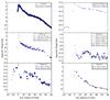 |
Fig. 1 Example optical light curves for 6 out of the 75 inspected novae. Observations reported by different telescopes and observers are shown in different colors. |
2. Optical nova catalog
We compiled a list of 75 optical novae from Astronomer’s Telegrams (ATels)1, the Central Bureau for Astronomical Telegrams (CBETs)2, the International Astronomical Union Circulars (IAUC)3, and a catalog of novae published by the Optical Gravitational Lensing Experiment (OGLE) team (Mróz et al. 2014, 2015) in the time range from August 2008 to the end of 2015. Additional light-curve information has been collected from the American Association of Variable Star Observers (AAVSO)4 and the Small and Medium Aperture Telescope System (SMARTS)5 (Walter et al. 2012).
We used the light curves to estimate the optical peak time and optical peak apparent magnitude for each novae (see Table A.1). There are many cases with a single optical peak around the discovery and a smooth subsequent decline. Many cases also have multiple peaks, with some cases where later peaks are modestly brighter, thus the latter dates are quoted (e.g., V1369 Cen 2013; V5668 Sgr 2015). Example light curves are shown in Fig. 1. A full list of novae including the optical peak information is shown in Table A.1. Other nova lists by Bill Gray6 and Koji Mukai7 have been checked for consistency with our list for the time window of August 2008 to the end of 2015. All novae in these lists are included in our list. Our list has a few additional sources, for instance, from the OGLE survey.
Not all light curves are sufficiently well sampled to allow an accurate determination of the peak time and optical peak apparent magnitude. These are excluded in some of our later studies. In addition to the peak time, we also estimated t2, the time during which the visual light curve fades by 2 mag from the maximum (Payne-Gaposchkin 1964). Again, not all light curves allowed the estimate of t2. For the known gamma-ray novae, we do not find a correlation between t2 and the duration of the gamma-ray emission (see Fig. 2).
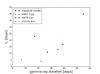 |
Fig. 2 Duration of > 100 MeV gamma-ray emission as a function of t2 for the gamma-ray detected novae (candidates). |
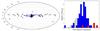 |
Fig. 3 Novae selected in a time range from August 2008 to the end of 2015. Left: spatial distribution in Galactic coordinates of the novae listed in Table A.1. Previously detected gamma-ray novae are shown in red. Right: optical peak apparent magnitude distribution of the novae, magnitudes of the five out of the six previously detected gamma-ray novae are overlaid in red. The peak magnitude of V959 Mon is not included because it has not been measured since the nova was too close to the Sun to be observed during its outburst. Most magnitudes are in V band. Peak magnitudes of novae that were only observed in I band are displayed by striped bars. |
As expected, the spatial distribution of novae peaks in the Galactic bulge region and along the Galactic plane (see Fig. 3, left). A slight asymmetry shows up in the spatial distribution of novae in the bulge. More novae are discovered at negative than at positive latitudes, which is likely due to the non-uniform exposure of the OGLE experiment (see Fig. 9 of Mróz et al. 2015). There are three outliers with a Galactic latitude of | b | > 15°: KT Eri 2009, U Sco 2010, and V965 Per 2011 at latitudes of − 32.0°, 21.9°, and 17.9°, respectively.
The optical peak apparent magnitude distribution is shown in the right panel of Fig. 3.
Note that more gamma-ray novae have been detected in 2016, but they are not included in this work (see, e.g., Li et al. 2016; Cheung et al. 2016a).
3. Gamma-ray data analysis
The Fermi-LAT is a pair-conversion telescope sensitive to gamma rays with energies from 20 MeV to greater than 300 GeV (Atwood et al. 2009). It has a large field of view and scans the entire sky every three hours. The LAT has been operated continuously since August 2008. Thus it is very well suited for searches for transient gamma-ray signals on the timescale of days to weeks.
In this analysis we used 7.4 years of Fermi-LAT data recorded from the start of operations in 2008 August 4 to 2015 December 31 (Fermi Mission Elapsed Time 239557418–473212804 s), restricted to the Pass 8 Source class8. We select the standard good time intervals (e.g., excluding time intervals when the field of view of the LAT intersected the Earth). The Pass 8 data benefit from improved reconstruction and event selection algorithms with respect to the previous data release Pass 7, leading to a significantly improved angular resolution and sensitivity (Atwood et al. 2013). To further increase the sensitivity, Pass 8 allows the division of the data set into four point-spread function (PSF) classes that can be used in a joint likelihood analysis (see Ackermann et al. 2015, for more details). The PSF classes are called PSF0, PSF1, PSF2, and PSF3, where PSF3 has the best and PSF0 the poorest angular resolution.
3.1. Method
We performed a binned analysis (i.e., binned in space and energy) using the standard Fermi-LAT ScienceTools package version v10r01p01 available from the Fermi Science Support Center9 (FSSC) and the P8R2_SOURCE_V6 instrument response functions. We analyzed data in the energy range of 100 MeV to 100 GeV binned into 24 logarithmic energy intervals equally spaced in log. We restricted the class PSF0 to the energy range of 1 GeV to 100 GeV to avoid using a very large region of interest (ROI) that contains events with very poor angular resolution. We note that these events do not contribute significantly to the detection significance. To minimize the contamination from the gamma rays produced in the Earth’s upper atmosphere, we applied a zenith angle cut of θ< 100° for PSF0 (note that the restricted energy range for PSF0 allowed us to use a relaxed zenith cut), θ< 85° for PSF1, θ< 85° for PSF2, and θ< 90° for PSF3, following in the recommendations of the Fermi-LAT collaboration. The effect of energy dispersion is included in the fits performed with the Fermi-LAT ScienceTools.
Analysis of known gamma-ray novae with Pass 8.
For each source and each time window, we selected a 10° × 10° ROI centered on the source position binned in  size pixels. The binning was applied in celestial coordinates, and an Aitoff projection was used. We constructed a model whose free parameters were fit to the data in the ROI. This model includes a point source at the nova position; its gamma-ray spectrum is represented as a power-law function with exponential cutoff, which was found to describe the spectra of the gamma-ray novae well (Ackermann et al. 2014),
 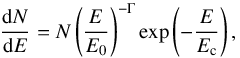 (1)with normalization N, energy cutoff Ec, and photon index Γ. The energy scale was fixed to E0 = 1 GeV. In addition, we modeled the background point-sources in the ROI and the isotropic and Galactic diffuse gamma-ray emission. We used preliminary versions of the Pass 8 Galactic interstellar emission model and the isotropic spectral template, which slightly differ from the versions published by the Fermi-LAT collaboration. The spatial model of the Galactic interstellar emission model we used is similar to the published one, while the spectral shape of both the Galactic interstellar emission model and the isotropic spectral template shows a small relative deviation of ~ 5%. We verified that the results are unchanged if the official versions for the Pass 8 Galactic interstellar emission model gll_iem_v06.fits10 (Acero et al. 2016b) and the isotropic spectral template iso_P8R2_SOURCE_V6_PSF0_v06.txt, for PSF0 and the equivalent models for the other PSF classes, are used. We included in the model 3FGL sources (Acero et al. 2015) within a larger region of 15° × 15° to account for the contribution of sources outside the ROI that leak into our selection because of the broad PSF. First we refit the spectral parameters of all background sources. Then we fixed all sources except for the normalization of sources within 3° from the nova position.
3.2. Analysis of known gamma-ray novae: unified spectrum
We repeated the analysis of the six known gamma-ray novae with the Pass 8 data set to develop a unified analysis strategy that could then be applied to the complete catalog of optical novae described in Sect. 2. We used a similar gamma-ray search time window as was used in the Pass 7 analysis (Ackermann et al. 2014; Cheung et al. 2016b).
We modeled the nova energy spectrum with a power-law function with an exponential cutoff (see Eq. (1)), where we allowed all spectral parameters (except for E0) to be free in the fit. The resulting best-fit spectral parameters and test statistic value for the six novae are summarized in Table 1. The test statistic, TS, is defined as follows (Mattox et al. 1996):  (2)where ℒ0 is the likelihood evaluated at the best-fit parameters under a background-only null hypothesis, that is, a model that does not include a point source at the nova position, and ℒ the likelihood evaluated at the best-fit model parameters when including a candidate point-source at the nova position. When including a candidate source adds one degree of freedom to the model one can interpret
  as the number of σ of a normal distribution.
The gamma-ray spectral parameters were the same for all novae within the statistical errors, except for the symbiotic nova V407Cyg, which has a harder spectrum (i.e., a lower photon index). In symbiotic novae, the dense wind of the red giant companion might influence the process of particle acceleration, explaining the different spectral behavior from the classical novae. All the Pass 8 derived spectral parameters are consistent with the previous Pass 7 results.
At low energies, systematic uncertainties introduced by modeling the Galactic diffuse emission become important. To estimate these uncertainties, we repeated our analysis using the alternative diffuse models introduced in Acero et al. (2016a). We found that the choice of diffuse emission model has a very mild effect on the best-fit spectral parameters shown in Table 1, which is negligible within the relatively large statistical errors. The resulting spectra are shown in Fig. 4.
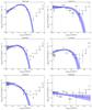 |
Fig. 4 Spectra from the six previously detected gamma-ray novae. The spectral energy distribution (SED) points including statistical uncertainties derived with the standard Galactic diffuse model are shown as black crosses, and a power law with exponential cutoff fit to that data is shown in blue. We show data points for bins with TS> 4, otherwise, we show 95% upper limits. The systematic uncertainties introduced by modeling the Galactic diffuse emission are estimated by repeating the analysis with alternative diffuse models. The envelope of the results using the alternative models are shown as gray bands for each energy bin. For V5668 Sgr, the fit did not constrain the cutoff energy, and we therefore present the results of a simple power-law fit. |
Since the spectral parameters are similar, we can assume that the spectral shape is the same for all novae. In the following, we combine all novae (including and excluding V407 Cyg) in a joint likelihood analysis tying the photon index and the cutoff energy across all novae, that is, while the normalization for each nova is a free parameter, only one common index and one common cutoff are fit. The results of the combined fit with a tied index and cutoff are also shown in Table 1. For the classical novae, the combined fit resulted in Γ = 1.90 ± 0.08 and Ec = 4.3 ± 1.2 GeV. To reduce the degrees of freedom in the unified analysis that was applied to all novae from the catalog, we fixed the index and cutoff energy to 1.9 and 4 GeV, respectively.
We applied a sliding time window analysis to the known novae using four different time windows of length 5, 10, 15, and 20 days to evaluate the optimal time window length, which was then applied in the unified approach to all novae of the catalog. The analysis was performed in a time window of a given length. The time window was then moved by 2 days, and the analysis was repeated. This produced a light curve with overlapping time bins. For each of the six novae, we repeated a sliding time window analysis for the four different time windows. The results are shown in Fig. 5. The 15 day or 20 day time windows generally yield the largest TS. We decided to perform the unified analysis with a 15 day time window.
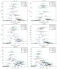 |
Fig. 5 TS for sliding time windows of different length for the six known gamma-ray novae. The x-axis shows the time relative to the optical peak time tpeak. In the case of V959 Mon, the gamma-ray peak was used. |
3.3. Search for gamma-ray emission from all novae in the catalog: sliding time window analysis
Given the optimized time window of 15 days and the spectral parameters provided by the joint likelihood analysis of the known gamma-ray novae, we then applied a sliding time window analysis to all novae of our catalog to search for gamma-ray emission in a unified approach.
We modeled the novae gamma-ray spectrum with a power-law function with an exponential cutoff with the normalization free to vary and fixed index and energy cutoff to the parameters obtained above (Γ = 1.9 and Ec = 4 GeV).
For each nova, we searched for gamma-ray emission in a sliding time window of 15 day length, motivated by the study of different time window lengths of the known gamma-ray novae presented above. The time window was moved in 2 day steps, starting from 60 days before the peak time to ending 75 days after the peak time. We considered the time windows starting 20 days before and 20 days after the peak time the signal region. Time windows more than 60 days before and more than 75 days after the peak time were considered our off-time region, where no signal is expected, and were used to study background fluctuations (see Fig. 6). To avoid contamination of the off-time region with signal (e.g., when the peak time could not be determined accurately from the optical light curve), we did not include the time windows 60 to 20 days before the peak and 20 to 75 days after the peak time.
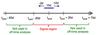 |
Fig. 6 Sketch of the sliding time window analysis. The start time of the time window is shifted in 2 day steps from 20 days before the peak time to 20 days after the peak time, i.e., the time window center moves from − 12.5 to 27.5 days relative to the peak time. |
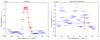 |
Fig. 7 Measured flux (TS> 4, shown in red) above 100 MeV and flux upper limits (shown in blue) for the various sliding time windows for the two novae V339 Del (left) and OGLE-2012-NOVA-01 (right). V339 Del is one of the previously known gamma-ray novae, while no gamma-ray emission was found for OGLE-2012-NOVA-01. |
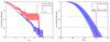 |
Fig. 8 Left: cumulative density of the TSmax distribution for the on-time (red) and off-time regions (blue) including only sources with TSmax< 25. Dotted (dashed) lines show the Gaussian equivalent one-sided 3σ (2σ) probability of finding a larger TS than the TS indicated by the intersection of the dashed line with the blue distribution. The dash-dotted line shows the 2σ probability after correction for trials. Right: sum of TS values for 69 novae. The value of the on-time data is shown as a red line, while the off-time data are shown in blue. The shaded blue band reflects the uncertainty introduced by the limited statistics of the off-time sample. |
In Fig. 7 we show the sliding time window results for two cases: V339 Del, which is one of the known gamma-ray novae, and OGLE-2012-NOVA-01, for which no gamma-ray emission was found. We display flux measurements with a TS larger than 4 as data points in Fig. 7, while less significant detections are shown as flux upper limits at 95% confidence level (CL), indicated by blue arrows as adopted by Ackermann et al. (2014) and Cheung et al. (2016b).
4. Results
4.1. Nova ensemble
All six previously known gamma-ray novae are found in the analysis of the individual sources, and because of the increased sensitivity with the Pass 8 data set, they are predominantly discovered with higher significance. However, no significant gamma-ray emission was found for any additional nova except for two new candidates at 2σ level (see Sect. 4.2).
To evaluate the significance of an excess, we repeated the sliding time-window analysis in the off-time region. Similar to the on-time analysis, we defined a random peak time in the off-time region and performed a sliding time window analysis in 2 day steps starting 20 days before the assigned peak time and ending 20 days after. In each case, we report the time window with the largest TS (defined according to Eq. (2)) out of all tested time windows, TSmax. We compare the TSmax distribution from the on-time and off-time region in Fig. 8 (left).
We used the off-time distribution to determine the 2σ and 3σ levels: the probability to obtain a TSmax> 14.5 (9.0) from background fluctuations is 0.13% (2.3%) (corresponding to 3(2)σ in a normal distribution). Testing several novae introduces a trials factor, which we accounted for by dividing the needed probability by the number of novae in our catalog (we used 69, excluding the 6 known gamma-ray novae). The corrected probability corresponding to the 2σ level is 0.03%. A TSmax> 18.0 is needed to reach the trial-corrected 2σ level.
In an attempt to find a sub-threshold population of novae, we performed a stacking analysis of all sub-threshold novae. Since the novae were fit independently, the stacking becomes a simple sum of TS values, TSsum. We removed the 6 known gamma-ray novae and summed the TS of the remaining 69 novae. We repeated this analysis 100 000 times on the off-time data by randomly picking 69 TS values from the blue distribution shown in Fig. 8 (left) and adding them. The distribution of the background TSsum values is shown in Fig. 8 (right) compared to an on-time value of TSsum = 249.5. To estimate the uncertainties introduced by the limited statistics of the off-time sample, we split the off-time sample in half. For each half, we repeated the procedure of randomly picking 69 novae 100 000 times. The results of the two halves represent the envelope of the shaded blue band shown in Fig. 8 (right). Including these uncertainties, we find a 3σ effect, indicating the existence of a sub-threshold gamma-ray nova population. When we exclude the three symbiotic novae (V745 Sco, V1534 Sco, and V1535 Sco, see also Sect. 4.5), the significance decreases to 2.5σ.
The known gamma-ray detected novae indicate an onset of the gamma-ray emission coincident or delayed by a few days with respect to the optical peak. A delay could be caused by absorption of the gamma rays via photon-atom interactions in an initially dense ejecta. Gamma rays appear once the density drops and the ejecta becomes transparent. Figure 9 shows a histogram of the time difference between the central time of the time window with maximum TS and the optical peak time. The time difference can vary from − 12.5 to 27.5 days relative to the peak. For the background, the distribution is expected to be flat. We note that novae with TS larger than 14.5 tend to reach the maximum TS closer to the optical peak time.
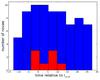 |
Fig. 9 Histogram of the time difference between the central time of the time window with maximum TS and the optical peak time (including all novae in our sample). The time difference can vary from − 12.5 to 27.5 days relative to the peak. Novae with a maximum TS smaller than 14.5 are shown in blue, sources with larger TS are plotted in red. |
4.2. Gamma-ray nova candidates
In addition to the six known gamma-ray emitting novae, we found two candidates with TSmax> 14.5 (i.e., 3σ before trials): V679 Car 2008 has a TSmax of 17.6, and V1535 Sco 2015 a TSmax of 17.2 (see Fig. 10). These values barely reach the trial-corrected 2σ level. Because these two candidates show the highest TS in the individual source analysis, they also dominate the sum of TS. The TS map for both candidates in the 15 day time window with maximum TS is shown in Fig. 11.
Spectroscopic observations identified V679 Car as a classical nova. Its spectrum is dominated by broad emission lines of the Balmer series and of Fe II emission features (Waagen et al. 2008). V1535 Sco is a symbiotic system (Srivastava et al. 2015, see also Sect. 4.5), similar to V407 Cyg. Hard, absorbed X-rays and synchrotron radio emission were detected at the early phase of the outburst indicating that the nova is produced by a white dwarf embedded within the wind of a red-giant companion (Walter 2015; Nelson et al. 2015). Linford et al. (2017) show that the measured X-ray emission indicates the presence of strong shocks during the first two weeks of the nova’s evolution, which is expected for a nova ejecta expanding into a thick wind from a giant companion. A rebrightening in X-rays after ~ 50 days indicates the existence of a second shock possibly produced in collisions between multiple outflows within the ejecta. No gamma-ray emission was found coincident with the second shock.
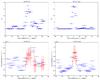 |
Fig. 10 Sliding time window results for V679 Car (left) and V1535 Sco (right). The upper row shows the TS value for each tested time window, while the lower row shows the measured flux above 100 MeV (TS> 4, red) or 95% flux upper limits (blue). |
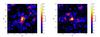 |
Fig. 11 TS map in the time window with maximum TS for V679 Car (left) and V1535 Sco (right). The white crosses indicate the point sources used in the model, i.e. the 3FGL background sources and the nova in the center. The black lines indicate the 3σ and 5σ contours. |
To obtain the duration of the nova candidates, we repeated the analysis for various start and stop times in 1 day time steps. We defined the duration from the time window that yielded the largest TS. Figure 12 shows the TS distribution as a function of start and stop time. For V679 Car, we obtain a duration of 35 days, and for V1535 Sco, it is 7 days.
The gamma-ray and optical light curve of the two candidate sources are shown in Fig. 13. The SED suffers from low statistics and is shown in Fig. 14. Table 2 lists the spectral fit parameters for the two candidates. The fit was applied in the energy range from 100 MeV to 100 GeV using the time window found in Fig. 12. Owing to small statistics, the errors on the fit parameters are large. Within the errors, the spectral parameters are similar to the spectra of the six known gamma-ray novae.
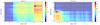 |
Fig. 12 TS as a function of start and stop time in days relative to the peak time for V679 Car (left) and V1535 Sco (right). The maximum TS is marked with a black circle. |
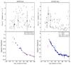 |
Fig. 13 Optical (bottom) and gamma-ray (top) light curves of V679 Car (left) and V1535 Sco (right). The gamma-ray data are binned in one-day bins. For days with TS< 4, we show 95% upper limits. |
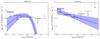 |
Fig. 14 SED for V679 Car (left) and V1535 Sco (right) using the duration obtained from Fig. 12. Both SEDs suffer from small statistics. The SED points derived with the standard Galactic diffuse model are shown as black crosses, and a power law with an exponential cutoff fit to these data is shown in blue. For V1535 Sco, the energy cutoff is not well constrained by the fit, and we therefore present the results of a simple power-law fit. The systematic uncertainties introduced by modeling the Galactic diffuse emission are estimated by repeating the analysis with alternative diffuse models. The envelopes of the results using the alternative models are shown as gray bands for each energy bin. |
We estimated the distance of V679 Car and V1535 Sco using two steps. First, we used the maximum magnitude versus rate of decline (MMRD) relationship, which provides an estimate of the maximum absolute magnitude as a function of t2 (Della Valle & Livio 1995; Downes & Duerbeck 2000). We note that other authors (e.g., Kasliwal et al. 2011) found the MMRD to be an oversimplification. Second, we used the extinction derived from the reddening E(B−V) measurements (SMARTS). With maximum magnitudes of 7.6 and 8.2 mag, t2 = 14 and 6 days, and extinctions of 3.72 and 2.81 mag, we estimated distances of (2.9 ± 0.7) and (7.3 ± 1.7) kpc for V679 Car and V1535 Sco, respectively. We note that our distance estimate of V1535 Sco is compatible with the Galactic center distance of ~ 8.5 kpc, which was also suggested by Linford et al. (2017).
We calculated the total number of gamma-ray photons and the total energy emitted by the two novae candidates. We note that the number of photons strongly depends on the spectral shape, which is not well constrained at low energies. The total energy is more robust to uncertainties in the spectral shape at low energies. Cheung et al. (2016b) suggested a relation between the total emission duration and the total energy of classical novae. While the classical nova V679 Car is in agreement with this relation, the symbiotic nova V1535 Sco emitted less energy than expected from the relation (see Fig. 15).
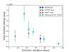 |
Fig. 15 Total emitted energy above 100 MeV as a function of the duration of the gamma-ray emission. Classical novae are marked with a circle and symbiotic novae with a triangle. The classical novae V679 Car is in agreement with the suggested relation between the total emission duration and the total energy of classical novae, while the symbiotic nova V1535 Sco emitted less energy than expected from the relation. |
New gamma-ray nova candidates.
4.3. Correlation of gamma-ray flux and optical light-curve properties
We studied the correlation of gamma-ray and optical flux with our nova sample. Eighteen sources with a large uncertainty on the optical apparent peak magnitude were excluded from this study. Figure 16 (left) shows the gamma-ray flux as a function of the optical apparent peak magnitude. No correlation is found. We note that the magnitudes are not corrected for extinction and can thus only be interpreted as upper limits on the real magnitude and lower limits on the real flux (Metzger et al. 2015). Two bright novae, T Pyx and KT Eri, with optical apparent peak magnitudes of 6.1 and 5.4, respectively, were not detected in gamma-rays.
Figure 16 (right) shows t2 as a function of the optical apparent peak magnitude. No correlation is found. The 18 sources with a large uncertainty on the optical apparent peak magnitude were excluded, and an additional 5 sources were excluded because the poorly sampled light curve did not allow us to estimate t2.
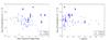 |
Fig. 16 Correlation of the gamma-ray flux with the optical peak apparent magnitude (left) and t2 (right): sources with TS> 14.5 (corresponding to 3σ) are shown as blue circles, while known gamma-ray novae are indicated as stars. Note that V959 Mon is not included because the peak was not covered by optical observations. Less significant sources are shown as upper limits indicated by arrows. The peak magnitude is measured in V band for most cases (shown in blue), but for a few cases, only I-band data were available (shown in green). |
4.4. Flux-distance relationship
Some of the novae in our catalog have a distance estimate reported in the literature. We list them in Table 3. The most reliable distance estimates stem from parallax measurements of the angular expansion of the nova shell several years after its outburst. However, such a measurement is only available for two novae in our sample, V959 Mon (Linford et al. 2015) and V339 Del (Schaefer et al. 2014). We note that Linford et al. (2015) combined the radio-interferometric expansion rate with the optical spectroscopic velocity measurement, which might lead to uncertainties when the radio and optical wavelength data are produced in different emission regions. Another method relies on the Galactic reddening-distance relation for the line of sight of the nova and its independent reddening measure (Özdönmez et al. 2016).
The gamma-ray flux as a function of distance is displayed in Fig. 17. Most gamma-ray novae are nearby with distance estimates ≤ 4.5 kpc, with the exception of the gamma-ray nova candidate V1535 Sco at a distance of 7.3 ± 1.7 kpc. We note that the distance for V1535 Sco was estimated with the MMRD method, whose justification was questioned by Kasliwal et al. (2011). We note that Finzell et al. (2015) found a larger distance of > 6.5 kpc for V1324 Sco than the 4.3 ± 0.9 kpc from Özdönmez et al. (2016) used here. If we had adopted this larger distance estimate, V1324 Sco would be added to the exception of gamma-ray bright but distant novae.
Not all nearby novae have been detected in gamma rays. V2672 Oph, V496 Sct, and V2674 Oph are closer than 4 kpc, but show no gamma-ray flux at the level of 2 × 10⁻⁷ cm-2 s-1. The luminous red nova, V1309 Sco (see Sect. 4.6), at a distance of 2.5 ± 0.4 kpc was not detected in gamma rays either, indicating that the gamma-ray flux is lower than 10-7 cm-2 s-1.
Using the subset of novae with a distance estimate, we investigated the gamma-ray luminosity, Lγ as a function of the optical peak apparent magnitude and t2 (see Fig. 18).
Distance estimates of a subset of novae from our catalog.
4.5. Recurrent and symbiotic novae
Symbiotic novae have an evolved companion (e.g., red giant) with a dense wind as opposed to a main-sequence companion for classical novae. Recurrent novae (see Schaefer 2010b; Mukai 2015, for a review) have undergone several outbursts over the past century (with typical time intervals between outbursts of 10 to 100 years). All novae might be recurrent given enough time. The time between outbursts is thought to be shorter for more massive white dwarfs, which makes recurrent novae candidate progenitors of Type Ia supernova (Patat 2013).
The first Fermi-LAT gamma-ray detection of a nova was made in the symbiotic-like nova V407 Cyg in 2010. Because the dense wind of the evolved companion star is interacting with the ejecta of the exploding white dwarf, the LAT emission duration can be more directly related to the specific parameters of the binary systems (e.g., separation). Although such systems are relatively rare, with ~10 known symbiotic novae known, LAT gamma-ray observations of other symbiotic systems with outbursts during the Fermi mission could thus be examined separately from the classical novae. Our sample contains three additional confirmed symbiotic novae: V745 Sco, V1534 Sco (Joshi et al. 2014), and V1535 Sco (Walter 2015). For three novae in our sample, several historical outbursts have been observed. These recurrent systems are V745 Sco (also a symbiotic system), T Pyx, and U Sco, which likely have main-sequence companions (Shore et al. 1994). Gamma-ray light curves of the recurrent and symbiotic novae are displayed in Fig. 20 for V745 Sco and for the other sources in Appendix B.
In the symbiotic recurrent novae V745 Sco, which had an outburst on 2014 Feb. 6.694 (CBET 3803; Waagen et al. 2014), preliminary 2 and 3 σ significances on Feb. 6 and 7 were reported (Cheung et al. 2014). This apparent short gamma-ray emission duration compared to V407 Cyg could be due to the fast onset of deceleration in the ejecta (Banerjee et al. 2014). With the new Pass 8 analysis, we confirm the low significances with TS = 6.5 and 5.6 on these days (see Fig. 20). We note that for V745 Sco, the Galactic center biased pointing strategy that (re)commenced on Feb 5.0 after a ToO pointing toward M82/SN2014J gave an optimized exposure at the nova position after the optical nova detection. The position of V1534 Sco 2014 also benefited from this exposure profile, although ~10 days after the novae (end of March 31, 2014), a ToO pointing of 3C 279 for 350 ks decreased the exposure at the nova position (Ciprini & Becerra Gonzalez 2014).
The recurrent nova T Pyx 2011 reached its optical peak on May 12, 2011, at 6.1 mag (see Chomiuk et al. 2014) and is thus one of the brightest sources that are non-detected in gamma rays. It shows a broad optical peak, which occurred unusually late, about one month after the optical discovery (April 14). Owing to the long duration of T Pyx, we decided to extend the sliding time window analysis to 60 instead of 20 days, but we did not find any excess of gamma rays at later times either (see Fig. 19). The recurrent nova U Sco peaks at 7.5 mag on January 28, 2010, but shows a narrow peak with t2 of only 2 days. Another relevant parameter in discussing the LAT-detectability of these systems are their distances. Despite their bright optical peaks, their estimated distance is quite large with 12.0 ± 2.0 kpc and 4.8 ± 0.5 kpc for U Sco and T Pyx, respectively (Schaefer 2010a; Sokoloski et al. 2013). If their gamma-ray luminosities are scaled to any of the LAT-detected novae, we thus expect U Sco to be 7−36 and T Pyx to be 1−6 times fainter in the LAT band.
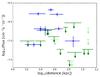 |
Fig. 17 Nova flux (blue) or flux upper limit (green) as a function of distance for a subsample of our catalog with estimated distances. Light green values indicate lower limits of the distance. |
4.6. Luminous red novae
Of the novae that have been optically discovered since the start of the Fermi mission, V1309 Sco 2008, which was not detected in gamma rays, deserves individual attention. It differs from the novae we discussed and can be classified as a luminous red novae, a subclass of eruptive stellar transients that are less luminous than traditional supernovae, but more luminous than classical novae. These transients might fill the luminosity gap between novae (absolute magnitude ranging between − 4 and − 10 mag) and supernovae (absolute magnitude range between − 15 and − 22 mag) (Kasliwal 2013). Another well-studied example is V838 Mon 2002 (Munari et al. 2002).
Several hypotheses have been proposed to explain the nature of outbursts in different luminous red novae. The most common model is a stellar merger (see, e.g., Nandez et al. 2014)11. Stellar mergers are common with rates of ~ 0.1/year for events more luminous than V1309 Sco (Kochanek et al. 2014).
Molnar et al. (2015) found that the contact binary star system KIC 9832227 at a distance of 565 pc shows an orbital period spiraling exponentially down to zero – similar to V1309 Sco before its outburst (Tylenda et al. 2011). They predicted that KIC 9832227 will merge and produce a red nova eruption in 2022.2 with an uncertainty of 0.7 years (Molnar et al. 2017). If Fermi is still operating at this time, it would be a unique opportunity to study a stellar merger 4.4 times closer than V1309 Sco.
5. Study of the gamma-ray emissivity distribution
In the following, we perform a population study with Monte Carlo simulations to set constraints on the properties of the gamma-ray emission of novae. Morris et al. (2017) initiated a similar population study with a simple flat gamma-ray emissivity model and were able to reproduce the rate of gamma-ray novae observed during eight years of Fermi-LAT mission (six novae in eight years were included in their analysis). The method we have developed slightly differs, and we compare several emissivity models (listed below), taking into account the new data listed in Appendix A. This subsection presents the method and the results that have to be considered as preliminary because the number of detected gamma-ray novae is low.
The aim is to reproduce the optical peak apparent magnitude, mmax, and gamma-ray flux, Fγ distribution of novae detected in optical and in gamma rays (see Fig. 16), assuming a gamma-ray emissivity (mean number of photons emitted per second in 15 days) distribution and taking into account the measured peak apparent magnitude distribution of all novae detected in optical from our list (see Fig. 3). We built parametrized models and fit their parameters to the observed distributions using a maximum likelihood method. Several emissivity models were tested, and their maximum likelihood values were compared to each other.
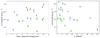 |
Fig. 18 Gamma-ray luminosity as a function of the optical peak apparent magnitude (left) and t2 (right). |
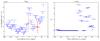 |
Fig. 19 Sliding time window results for T Pyx extended to 60 days. The left panel shows the TS value for each tested time window, while the right panel shows the measured flux above 100 MeV (TS> 4, red) or 95% flux upper limits (blue). |
The observed distributions Oall(mmax) and Oγ(mmax,Fγ) are built with the list of novae presented in Appendix A. However, novae discovered in the I band and V959 Mon (which has not been observed at peak magnitude) are not included in the Oall(mmax) distribution. V959 Mon is included in the Oγ(mmax,Fγ) distribution with an observed peak apparent magnitude of 5 as adopted in Ackermann et al. (2014, see references herein), as well as the two nova candidates in order to improve the already low statistics. In the following we assume that the gamma-ray emissivity model of symbiotic and classical novae is the same. The luminous red nova V1309 Sco has been excluded from the analysis (we note that including it does not change the results significantly).
The modeled distributions Mall(mmax) and Mγ(mmax,Fγ) were generated with Monte Carlo methods. The spatial distribution of novae in our Galaxy was based on the model proposed by Kent et al. (1991; see also Senziani et al. 2008; and Jean et al. 2000, for the method). Their absolute optical magnitude at maximum were distributed as a Gaussian distribution with a mean value of − 7.5 and a standard deviation of 0.8 (as in Shafter 2017), and their apparent maximum magnitudes were calculated with the extinction law of Shafter (2017). With this spatial distribution and a nova rate of ~ 50 yr-1 (Shafter 2017), the nova rate obtained in the bulge is ~ 16 yr-1 , which is in agreement with the rate of (13.8 ± 2.6) yr-1 measured by Mróz et al. (2015) with OGLE observations. The decision whether a simulated nova with an apparent peak magnitude mmax is detected was taken according to a parametrized probability function (see below).
The set of these simulated novae was used to calculate the Mall(mmax) distribution. By fitting the model to the observed distribution Oall(mmax), we obtained the likelihood λall. We computed the function Λall = −2ln(λall), which depends on the Galactic nova rate and on the parameters of the probability function. For each simulated nova, the mean gamma-ray flux in a 15 day time window, Fγ, was calculated with the emissivity model and its distance. The decision whether a nova is detected in gamma-ray was obtained with a bootstrap method using the upper-limit fluxes listed in Appendix A. It has to be noted that the probability to detect the gamma-ray flux from a nova does not depend on its Galactic coordinate as in Morris et al. (2017), since we did not observe a significant correlation of upper-limit fluxes with Galactic longitudes with our list of novae. The modeled distribution Mγ(mmax,Fγ) was built with the set of simulated novae that are detected in optical and in gamma rays. This allowed us to obtain the likelihood function Λγ taking into account the observed distribution Oγ(mmax,Fγ). Λγ depends on the Galactic nova rate, the parameters of the probability function, and the parameter of the emissivity model. The combination of the two likelihood functions yields the total likelihood function: Λtot = Λall + Λγ. The first term takes into account the uncertainties in the Galactic rate of novae and the probability to detect them. The second term evaluates the quality of the fit of the emissivity model to the data.
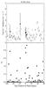 |
Fig. 20 Upper (lower) panel: flux (TS) vs. time relative to tpeak for V745 Sco in one-day bins. No data are available from this position in the sky a few days before the peak because of a pointed observation of the LAT to observe M82. |
As the Galactic nova rate and their probability of detection in optical are highly uncertain (e.g., see Shafter 2017), the parameters of a detection probability law were fit to the optical peak apparent magnitude distribution, Oall(mmax) for each gamma-ray emissivity model. For simplicity, we assumed that the probability to detect a nova follows a decaying exponential law of the peak magnitude such that the probability to detect bright novae is maximum and the probability decreases when the brightness decreases. The parametrized detection probability law is the analytical function p0 × e− (mmax−p1) /p2 , where p0 is a completeness factor to take into account that even bright novae can be missed in optical (see Shafter 2017), p1 a magnitude shift, and p2 a magnitude cutoff. When mmax<p1, the function value is p0. There is a degeneracy between the Galactic nova rate and the completeness factor since the same optical peak apparent magnitude distribution can be obtained with a high or low nova rate and a low or high completeness factor. Therefore, in the combined likelihood analyses, the parameter that was fit to the data was νnovae × p0, the product of the completeness factor (p0) with the Galactic nova rate (νnovae).
Results of the maximum likelihood analyses.
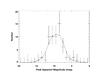 |
Fig. 21 Measured distribution of the optical peak apparent magnitudes and best-fitting PLslope2 model. The Poissonian (1-σ) error bars are calculated with the method described by Gehrels (1986). |
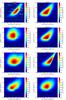 |
Fig. 22 Best-fitting gamma-ray flux: optical peak apparent magnitude distributions of several gamma-ray emissivity models (see text). The observed gamma-ray novae are overplotted for comparison. |
As the origin of the gamma-ray emission is not yet known, we considered several emissivity distributions modeled by simple functions. Except for the Constant model (see below), the emissivity distributions were chosen such as to reproduce the wide range of measured emissivities and to search for a possible link with the maximum absolute magnitude of novae. The emissivity models tested in this analysis are (pγ for each model is in units of 1038 ph/s):
-
Constant: the mean emissivity in 15 days is thesame for all novae. The parameterpγ,Constant is the mean emissivity.
-
Uniform: the mean emissivity is randomly distributed according to a uniform distribution from zero to the maximum value, pγ,Uniform.
-
10 Gauss: the logarithm of the mean emissivity is distributed as a Gaussian with a mean value log 10(pγ,10Gauss) and a standard deviation of 1 (see the end of this section for a discussion of the standard deviation value).
-
Gaussian: the mean emissivity is distributed as an absolute value of a Gaussian distribution centered on zero ph/s. The parameter pγ,Gauss is the standard deviation of the Gaussian.
-
PLslope2: the mean emissivity is distributed as a power-law distribution with a slope of 2 (see the discussion on the slope value at the end of this section). The parameter pγ,PL2 is the minimum emissivity of the power law.
-
CorrelMv: the mean emissivity is (correlated with) proportional to the maximum luminosity in optical. The emissivity is equal to pγ,CorrelMv × 10(| Mmax | −7.5)/2.5. The parameter pγ,CorrelMv is the mean emissivity when the maximum absolute magnitude is − 7.5.
-
AnticorMv: the mean emissivity is (anticorrelated with) inversely proportional to the maximum luminosity in optical (e.g., see Fig. 18). The emissivity is equal to pγ,AnticorMv × 10− (| Mmax | −7.5)/2.5, with Mmax the absolute maximum magnitude. The parameter pγ,AnticorMv is the mean emissivity when the maximum absolute magnitude of the nova is − 7.5. We discuss alternative AnticorMv models at the end of this section.
Table 4 presents the results of the likelihood analyses with the best-fit emissivity parameters, the mean rate of novae detected in optical and in gamma rays, and the mean rate of novae detected in gamma rays alone. The latter mean rate is highly uncertain, however, taking into account the large uncertainty on the Galactic nova rate. Figure 21 shows the measured distribution of peak apparent magnitudes and the corresponding best-fit distribution of the PLslope2 model obtained by minimizing χ2 (Λall value of 53.5 for a number of degrees of freedom of 48). The best-fitting emissivity distribution models are PLslope2, AnticorMv, and 10 Gauss. The difference in Λtot values of these three models are not large enough (significances ≲2σ) to favor one of them over the others. The difference in Λtot of the four other models compared to PLslope2 model are ≳16 (i.e., significance > 4σ). They cannot explain the observed distribution and can be rejected. We note that the constant model (which is equivalent to a standard candle model) can be rejected by comparing the gamma-ray emissivities of novae derived from the measured mean fluxes and distances (see Table 3; the difference in emissivity increases to a factor of ~30). The rate of novae detected in optical and in gamma rays listed in Table 4 agrees with the observed rate of ~1 yr-1. The rate of novae detected in gamma rays alone, obtained with the three best-fit models, ranges from 1.4 yr-1 to 5.0 yr-1, taking into account uncertainties. These novae are not discovered in optical either because they are not observable (completeness effect; e.g., as the case of V959 Mon, which was too close to the Sun to be discovered when it was at its peak apparent magnitude) or their peak apparent magnitude is too faint to be discovered, as is the case of novae in the bulge region. With the three best-fitting models, the detection rate of the gamma-ray emission from novae not discovered in optical within | l | < 9 deg ranges from 0.5 to 0.8 yr-1 (without taking into account the statistical uncertainty of the fit). The best-fitting peak apparent magnitude and gamma-ray flux distributions of the analyzed models are presented in Fig. 22 with the observed gamma-ray novae. The distributions of the poorer models show a rather strong correlation between the gamma-ray flux and the peak apparent magnitude, which is not the case for the three best-fitting models. The extent of the latter distributions is broader than the poorer modeled distributions and favor high gamma-ray flux from faint peak apparent magnitude novae. Novae with a peak apparent magnitude as faint as 10−12 mag can be detected in gamma rays12, in agreement with Morris et al. (2017), who estimated that novae with an R-band magnitude ≤ 12 and distance ~ 8 kpc are good candidates for a detection with the Fermi-LAT.
We investigated alternative versions of the best-fitting models. Maximum likelihood analyses were performed for several slopes of the emissivity power-law model. The best-fitting slope obtained is 2.01 , which is compatible to the slope of 2 used in the initial analysis (PLslope2 model). Similarly, the analysis made with the gamma-ray emissivity model inversely proportional to the power law of the maximum luminosity in optical (i.e., AnticorMvslope model), with the slope as a free parameter, yields a best-fitting slope value of 1.26
 , which is compatible to the slope of 1 used in the initial analysis (AnticorMv model).
The 10Gauss model uses a fixed standard deviation of 1. When the standard deviation is a free parameter, the maximum likelihood analysis results in a slightly better adjustment with a best-fit standard deviation of 0.63 and a Λtot of 147.7 (see the distribution for the model 10Gauss0.63 in Fig. 22).
We also tested an emissivity model similar to the model used by Morris et al. (2017), which assumed a gamma-ray emissivity uniformly distributed between the minimum and maximum values of the detected gamma-ray nova emissivities. This model is similar to the Uniform model, but with a non zero value for the lowest emissivity. The likelihood analysis yields a too high rate of novae detected in optical and in gamma rays of 2.6 yr-1 and a Λtot of 180.9, which corresponds to a difference of ~6σ compared to the PLslope2 Λtot value.
The results are not significantly changed (i.e., ΔΛtot ≲ 3) when other extinction models (e.g., the extinction model of Hakkila et al. 1997; as used in Senziani et al. 2008) are applied in the analyses or when a mean maximum absolute magnitude of − 7.2 is used instead of − 7.5 (see the discussion in Shafter 2017); the best-fitting completeness-corrected novae rate (νnovae × p0) changes slightly, but the other detection probability law parameters (p1 and p2) remain unchanged.
The optical peak apparent magnitude of V959 Mon was not measured as this nova was too close to the Sun during its outburst. We verified that the peak apparent magnitude uncertainty did not greatly affect the results of the analyses by fitting some emissivity models with an optical peak apparent magnitude of 3 instead of 5. The results did not change with the PLslope2 model. This is because the optical peak apparent magnitude shift results in a position of the nova in the mmax–Fγ diagram where the distribution value is similar (see Fig. 21). With the AnticorMv model, the Λtot increases from 150.1 to 151.7, but the best-fit parameters do not change significantly.
6. Summary and conclusion
We have systematically searched for gamma-ray emission from 75 novae. We confirmed the 6 previously known gamma-ray novae and found 2 additional candidates, which are found at 3σ significance (not including trial factors) but barely reach a 2σ significance after trial correction. V679 Car is a classical nova, while V1535 Sco is a symbiotic system. Their spectral characteristics and their duration are similar to the previously gamma-ray detected novae. If we consider the two candidates as detected, the observed rate of LAT-detected novae is about ~ 1 per year (8 novae in 7.4 years).
The paper presents the results of the analysis of novae discovered with their optical flux. It is not excluded that some novae, not discovered in optical (e.g., due to extinction), emit enough gamma-ray flux to be detected with Fermi-LAT. If they are bright enough, they should be found by the Fermi all-sky variability analysis (FAVA; Abdollahi et al. 2017), which searches for gamma-ray flares on the timescale of one week. Five flares of the second FAVA catalog have been associated with the gamma-ray bright novae studied in this paper. It is possible that some of the unidentified FAVA flares are produced by novae that were missed by optical surveys.
We provide the measured gamma-ray flux or flux upper limits for the non-detections. We find an indication at 3σ significance for a sub-threshold population of dim novae. No correlation of optical peak magnitude and gamma-ray flux was found. Non-detections in gamma rays can be caused by a too large distance, by absorption of the high-energy emission, or are due to an absence of particle acceleration in the nova. The provided gamma-ray flux upper limits will be useful for future modeling of physical processes taking place in novae.
We compared our measurements to simulated gamma-ray emissivity models and found that a power-law distribution with a slope of 2, an emissivity distribution inversely proportional to the maximum luminosity in optical, and a log-normal distribution of the emissivity match the data best. A constant emissivity (i.e., assuming novae are standard candles) can be rejected. In general, the best-fitting distributions are not extended enough compared to the observed distributions. The locations of detected gamma-ray novae are spread throughout the mmax–Fγ diagram. This suggests that the true emissivity distribution would/should be more complicated than the tested distributions. Moreover, we assumed that the emissivities of all gamma-ray novae originate from the same distribution, while it is not excluded that they differ with the chemical composition of the white dwarf (CO vs. ONe) and the type of nova (e.g., classical vs. symbiotic, see discussion in Sect. 4.5).
If this is the case, this analysis has to be made independently for each type of nova. Therefore, we cannot yet conclude on the gamma-ray emissivity distribution of novae.
Physical models of the gamma-ray emission combined with novae properties would allow us to build more reliable emissivity distributions that will be better constrained in the future with a larger sample of observed gamma-ray novae (i.e., larger statistics) and a finer/improved analysis (e.g., modeled distributions including the Galactic coordinates l,b of simulated novae and a more elaborate optical detection probability law).
The gamma-ray properties of the small number of LAT-detected novae (one symbiotic and five classical; see Table 1) plus the two new candidates presented here (one symbiotic and one classical; Table 2) and distances are not measured well enough to claim a firm difference in their emissivities. Observationally, their gamma-ray emission properties (spectra, light curves) are similar, which could suggest a common gamma-ray emission origin. However, as noted in Ackermann et al. (2014), small differences exist that could imply different emission mechanisms: (i) the power-law index of the V407 Cyg spectrum is lower than that of classical novae, but it is compatible with the index of V959 Mon taking into account the statistical uncertainties; and (ii) the gamma-ray onset of both symbiotic novae is coincident with the optical peak magnitude (see discussion in Sect. 4.5), while a delay is found in three of the classical novae, with one exception, where the gamma-ray onset of the classical nova V1324 Sco occurred before the optical peak. On the modeling side, the gamma-ray emission of the symbiotic nova V407 Cyg could be explained with an interaction between the ejecta and the dense wind of the secondary (Abdo et al. 2010; Martin & Dubus 2013), while internal shocks are favored to explain the emission of classical novae (Ackermann et al. 2014; Metzger et al. 2014). However, Martin et al. (2017) were recently able to reproduce the gamma-ray spectrum and light curve of V407 Cyg reasonably well with an internal shock model. Taking into account their recent results and the similarities in gamma-ray emission properties, it is possible that the gamma rays in symbiotic novae could be due to a combination of external and internal shocked emission. Further observations of gamma-ray novae would provide better statistics to separate the two populations of novae, as well as better measured characteristics to detect clear differences of their emissions.
Up to now, no VHE (> 0.1 TeV) gamma-ray emission was detected from novae (Ahnen et al. 2015; Aliu et al. 2012). Future optical surveys such as the All-Sky Automated Survey for Supernovae (ASAS-SN; Shappee et al. 2014) and the Zwicky Transient Facility (ZTF; Bellm 2014) will deliver more optical nova detections, which would allow an extended search for gamma-ray emission from these sources.
http://projectpluto.com/galnovae/galnovae.txt (accessed on March 1, 2017).
https://asd.gsfc.nasa.gov/Koji.Mukai/novae/novae.html (accessed on March 1, 2017).
We note that this implies that luminous red novae are not thermonuclear explosions, i.e., technically not novae. However, removing V1309 Sco from our analysis does not significantly change our results.
For instance, ~ 15% of novae detected in optical and in gamma rays have a peak apparent magnitude in the 10−12 range with the PLslope2 model.
Acknowledgments
We thank Justin Linford for spotting an inconsistency in the references of the quoted nova distance measurements.
The Fermi LAT Collaboration acknowledges generous ongoing support from a number of agencies and institutes that have supported both the development and the operation of the LAT as well as scientific data analysis. These include the National Aeronautics and Space Administration and the Department of Energy in the United States, the Commissariat à l’Énergie Atomique and the Centre National de la Recherche Scientifique/Institut National de Physique Nucléaire et de Physique des Particules in France, the Agenzia Spaziale Italiana and the Istituto Nazionale di Fisica Nucleare in Italy, the Ministry of Education, Culture, Sports, Science and Technology (MEXT), High Energy Accelerator Research Organization (KEK) and Japan Aerospace Exploration Agency (JAXA) in Japan, and the K. A. Wallenberg Foundation, the Swedish Research Council and the Swedish National Space Board in Sweden.
Additional support for science analysis during the operations phase is gratefully acknowledged from the Istituto Nazionale di Astrofisica in Italy and the Centre National d’Études Spatiales in France. This work performed in part under DOE Contract DE-AC02-76SF00515.
We acknowledge with thanks the variable star observations from the AAVSO International Database contributed by observers worldwide and used in this research.
A.F. was supported by the Initiative and Networking Fund of the Helmholtz Association.
Work by C.C.C. at NRL is supported in part by NASA DPR S-15633-Y and Fermi Guest Investigator program 14-FERMI14-0005.
References
- Abdo, A. A., Ackermann, M., Ajello, M., et al. 2010, Science, 329, 817 [NASA ADS] [CrossRef] [PubMed] [Google Scholar]
- Abdollahi, S., Ackermann, M., Ajello, M., et al. 2017, ApJ, 846, 34 [NASA ADS] [CrossRef] [Google Scholar]
- Acero, F., Ackermann, M., Ajello, M., et al. 2015, ApJS, 218, 23 [Google Scholar]
- Acero, F., Ackermann, M., Ajello, M., et al. 2016a, ApJS, 224, 8 [NASA ADS] [CrossRef] [Google Scholar]
- Acero, F., Ackermann, M., Ajello, M., et al. 2016b, ApJS, 223, 26 [NASA ADS] [CrossRef] [Google Scholar]
- Ackermann, M., Ajello, M., Albert, A., et al. 2014, Science, 345, 554 [NASA ADS] [CrossRef] [Google Scholar]
- Ackermann, M., Albert, A., Anderson, B., et al. 2015, PRL, 115, 231301 [Google Scholar]
- Ahnen, M. L., Ansoldi, S., Antonelli, L. A., et al. 2015, A&A, 582, A67 [NASA ADS] [CrossRef] [EDP Sciences] [Google Scholar]
- Aliu, E., Archambault, S., Arlen, T., et al. 2012, ApJ, 754, 77 [NASA ADS] [CrossRef] [Google Scholar]
- Atwood, W. B., Abdo, A. A., Ackermann, M., et al. 2009, ApJ, 697, 1071 [NASA ADS] [CrossRef] [Google Scholar]
- Atwood, W. B., Albert, A., Baldini, L., et al. 2013, ArXiv e-prints [arXiv:1303.3514] [Google Scholar]
- Ayani, K. 2010, CBET, 2186, 1 [NASA ADS] [Google Scholar]
- Ayani, K., & Tago, A. 2012, CBET, 3177, 1 [NASA ADS] [Google Scholar]
- Ayani, K., Murakami, N., Hata, K., et al. 2009, CBET, 1911, 1 [NASA ADS] [Google Scholar]
- Aydi, E., Mróz, P., Whitelock, P. A., et al. 2016, MNRAS, 461, 1529 [NASA ADS] [CrossRef] [Google Scholar]
- Banerjee, D. P. K., Joshi, V., Venkataraman, V., et al. 2014, ApJ, 785, L11 [NASA ADS] [CrossRef] [Google Scholar]
- Banerjee, D. P. K., Srivastava, M. K., Ashok, N. M., & Venkataraman, V. 2016, MNRAS, 455, L109 [NASA ADS] [CrossRef] [Google Scholar]
- Bellm, E. 2014, in The Third Hot-wiring the Transient Universe Workshop, eds. P. R. Wozniak, M. J. Graham, A. A. Mahabal, & R. Seaman, 27 [Google Scholar]
- Brown, N. J., & Samus, N. N. 2011a, CBET, 2796, 1 [NASA ADS] [Google Scholar]
- Brown, N. J., Samus, N. N., Guido, E., et al. 2011b, IAUC, 9228, 1 [NASA ADS] [Google Scholar]
- Cheung, C. C., Jean, P., & Shore, S. N. 2014, The Astronomer’s Telegram, 5879 [Google Scholar]
- Cheung, C. C., Jean, P., Shore, S. N., & Fermi Large Area Telescope Collaboration 2016a, The Astronomer’s Telegram, 9594 [Google Scholar]
- Cheung, C. C., Jean, P., Shore, S. N., et al. 2016b, ApJ, 826, 142 [NASA ADS] [CrossRef] [Google Scholar]
- Chomiuk, L., Nelson, T., Mukai, K., et al. 2014, ApJ, 788, 130 [NASA ADS] [CrossRef] [Google Scholar]
- Ciprini, S., & Becerra Gonzalez, J. 2014, ATel, 6036,1 [NASA ADS] [Google Scholar]
- Della Valle, M., & Livio, M. 1995, ApJ, 452, 704 [NASA ADS] [CrossRef] [Google Scholar]
- Downes, R. A., & Duerbeck, H. W. 2000, AJ, 120, 2007 [NASA ADS] [CrossRef] [Google Scholar]
- Elenin, L. 2009, CBET, 1900, 1 [NASA ADS] [Google Scholar]
- Finzell, T., Chomiuk, L., Munari, U., & Walter, F. M. 2015, ApJ, 809, 160 [NASA ADS] [CrossRef] [Google Scholar]
- Fujikawa, S., Yamaoka, H., & Nakano, S. 2012, CBET, 3202 [Google Scholar]
- Gehrels, N. 1986, ApJ, 303, 336 [NASA ADS] [CrossRef] [Google Scholar]
- Greiner, J., Kruehler, T., Schady, P., Rau, A., & Olivares, F. 2010, ATel, 2746, 1 [NASA ADS] [Google Scholar]
- Guido, E., Sostero, G., Maehara, H., & Fujii, M. 2009, CBET, 2053, 1 [NASA ADS] [Google Scholar]
- Hakkila, J., Myers, J. M., Stidham, B. J., & Hartmann, D. H. 1997, AJ, 114, 2043 [NASA ADS] [CrossRef] [Google Scholar]
- Hounsell, R., Bode, M. F., Hick, P. P., et al. 2010, ApJ, 724, 480 [NASA ADS] [CrossRef] [EDP Sciences] [Google Scholar]
- Itagaki, K., & Nakano, S. 2015, CBET, 4145, 1 [Google Scholar]
- Jean, P., Hernanz, M., Gómez-Gomar, J., & José, J. 2000, MNRAS, 319, 350 [NASA ADS] [CrossRef] [Google Scholar]
- Joshi, V., Ashok, N. M., & Banerjee, D. P. K. 2010, CBET, 2210, 1 [NASA ADS] [Google Scholar]
- Joshi, V., Banerjee, D. P. K., Venkataraman, V., & Ashok, N. M. 2014, ATel, 6032 [Google Scholar]
- Kabashima, F., Corelli, P., Guido, E., & Sostero, G. 2009, IAUC, 9089, 1 [NASA ADS] [Google Scholar]
- Kajikawa, T., Arai, A., Waagen, E. O., et al. 2013, CBET, 3556, 1 [NASA ADS] [Google Scholar]
- Kasliwal, M. M. 2013, in Binary Paths to Type Ia Supernovae Explosions, eds. R. Di Stefano, M. Orio, & M. Moe, IAU Symp., 281, 9 [Google Scholar]
- Kasliwal, M. M., Cenko, S. B., Kulkarni, S. R., et al. 2011, ApJ, 735, 94 [NASA ADS] [CrossRef] [Google Scholar]
- Kent, S. M., Dame, T. M., & Fazio, G. 1991, ApJ, 378, 131 [NASA ADS] [CrossRef] [Google Scholar]
- Kinugasa, K., Nishiyama, K., Kabashima, F., et al. 2009a, IAUC, 9041, 1 [NASA ADS] [Google Scholar]
- Kinugasa, K., Honda, S., Hashimoto, O., Taguchi, H., & Takahashi, H. 2009b, CBET, 1995, 1 [NASA ADS] [Google Scholar]
- Kinugasa, K., Takahashi, H., Honda, S., Taguchi, H., & Hashimoto, O. 2009c, CBET, 2076, 1 [NASA ADS] [Google Scholar]
- Kochanek, C. S., Adams, S. M., & Belczynski, K. 2014, MNRAS, 443, 1319 [NASA ADS] [CrossRef] [PubMed] [Google Scholar]
- Korotkiy, S., Sokolovsky, K., Brown, N. J., et al. 2012, CBET, 3089, 1 [NASA ADS] [Google Scholar]
- Kozlowski, S., Poleski, R., Udalski, A., et al. 2012, ATel, 4323, 1 [NASA ADS] [Google Scholar]
- Li, K.-L., Chomiuk, L., Strader, J., et al. 2016, The Astronomer’s Telegram, 9771 [Google Scholar]
- Liller, W., Tabur, V., Williams, P., et al. 2008a, IAUC, 8990, 2 [NASA ADS] [Google Scholar]
- Liller, W. 2008b, CBET, 1591, 1 [NASA ADS] [Google Scholar]
- Liller, W. 2008c, IAUC, 9004, 1 [NASA ADS] [Google Scholar]
- Liller, W. 2008d, IAUC, 9005, 3 [NASA ADS] [Google Scholar]
- Liller, W. 2010, CBET, 2264, 1 [NASA ADS] [Google Scholar]
- Linford, J. D., Ribeiro, V. A. R. M., Chomiuk, L., et al. 2015, ApJ, 805, 136 [NASA ADS] [CrossRef] [Google Scholar]
- Linford, J. D., Chomiuk, L., Nelson, T., et al. 2017, ApJ, 842, 73 [NASA ADS] [CrossRef] [Google Scholar]
- Lipunov, V., & Tyurina, N., et al. 2011, IAUC, 9247, 1 [NASA ADS] [Google Scholar]
- Maehara, H. 2010a, CBET, 2139, 1 [NASA ADS] [Google Scholar]
- Maehara, H. 2010b, CBET, 2142, 1 [NASA ADS] [Google Scholar]
- Maehara, H., Hirosawa, K., & Kabashima, F. 2010c, CBET, 2199, 1 [NASA ADS] [Google Scholar]
- Maehara, H. 2010d, CBET, 2205, 1 [NASA ADS] [Google Scholar]
- Martin, P., & Dubus, G. 2013, A&A, 551, A37 [NASA ADS] [CrossRef] [EDP Sciences] [Google Scholar]
- Martin, P., Dubus, G., Jean, P., Tatischeff, V., & Dosne, C. 2017, A&A, submitted [Google Scholar]
- Mattox, J. R., Bertsch, D. L., Chiang, J., et al. 1996, ApJ, 461, 396 [NASA ADS] [CrossRef] [Google Scholar]
- Metzger, B. D., Hascoët, R., Vurm, I., et al. 2014, MNRAS, 442, 713 [NASA ADS] [CrossRef] [Google Scholar]
- Metzger, B. D., Finzell, T., Vurm, I., et al. 2015, MNRAS, 450, 2739 [NASA ADS] [CrossRef] [Google Scholar]
- Molnar, L. A., Van Noord, D. M., Steenwyk, S. D., Spedden, C. J., & Kinemuchi, K. 2015, AAS, 225, 415.05 [Google Scholar]
- Molnar, L. A., Van Noord, D. M., Kinemuchi, K., et al. 2017, ApJ, 840, 1 [NASA ADS] [CrossRef] [Google Scholar]
- Morris, P. J., Cotter, G., Brown, A. M., & Chadwick, P. M. 2017, MNRAS, 465, 1218 [NASA ADS] [CrossRef] [Google Scholar]
- Mróz, P., Poleski, R., Udalski, A., et al. 2014, MNRAS, 443, 784 [NASA ADS] [CrossRef] [Google Scholar]
- Mróz, P., Udalski, A., Poleski, R., et al. 2015, ApJS, 219, 26 [NASA ADS] [CrossRef] [Google Scholar]
- Mukai, K. 2015, Acta Polytechnica CTU Proc., 2, 246 [NASA ADS] [CrossRef] [Google Scholar]
- Munari, U., & Dallaporta, S. 2010, CBET, 2185, 1 [NASA ADS] [Google Scholar]
- Munari, U., Henden, A., Kiyota, S., et al. 2002, A&A, 389, L51 [NASA ADS] [CrossRef] [EDP Sciences] [Google Scholar]
- Munari, U., Saguner, T., Ochner, P., et al. 2009a, CBET, 1912, 1 [NASA ADS] [Google Scholar]
- Munari, U., Saguner, T., Siviero, A., et al. 2009b, CBET, 1999, 1 [NASA ADS] [Google Scholar]
- Munari, U., Siviero, A., Valisa, P., et al. 2009c, CBET, 2034, 1 [NASA ADS] [Google Scholar]
- Munari, U., Henden, A., Valisa, P., Dallaporta, S., & Righetti, G. L. 2010a, PASP, 122, 898 [NASA ADS] [CrossRef] [Google Scholar]
- Munari, U., Ochner, P., Maitan, A., et al. 2012, CBET, 3184, 1 [NASA ADS] [Google Scholar]
- Munari, U., Ochner, P., Dallaporta, S., et al. 2014, MNRAS, 440, 3402 [Google Scholar]
- Munari, U., Henden, A., Banerjee, D. P. K., et al. 2015, MNRAS, 447, 1661 [NASA ADS] [CrossRef] [Google Scholar]
- Munari, U., Hambsch, F.-J., & Frigo, A. 2017, MNRAS, 469, 4341 [NASA ADS] [CrossRef] [Google Scholar]
- Nakano, S., & Fujii, M. 2012, CBET, 3182, 1 [NASA ADS] [Google Scholar]
- Nakano, S., & Nishimura, H. 2009, CBET, 2008, 1 [NASA ADS] [Google Scholar]
- Nakano, S., & Sakurai, Y. 2010, CBET, 2265, 1 [NASA ADS] [Google Scholar]
- Nakano, S., & Samus, N. N. 2013, IAUC, 9258, 1 [NASA ADS] [Google Scholar]
- Nakano, S., Nishiyama, K., Kabashima, F., & Sakurai, Y. 2008a, CBET, 1496, 1 [NASA ADS] [Google Scholar]
- Nakano, S., Nishiyama, K., Kabashima, F., et al. 2008b, IAUC, 8972, 1 [NASA ADS] [Google Scholar]
- Nakano, S., Yamaoka, H., & Kadota, K. 2009a, CBET, 1910, 1 [NASA ADS] [Google Scholar]
- Nakano, S., Yamaoka, H., Itagaki, K., et al. 2009b, IAUC, 9064, 1 [NASA ADS] [Google Scholar]
- Nakano, S., Nishimura, H., Guido, E., Sostero, G., & Kazarovets, E. V. 2009, IAUC, 9093, 1 [NASA ADS] [Google Scholar]
- Nakano, H., Nishimura, H., Itagaki, K., & Kadota, K. 2010a, CBET, 2128, 1 [NASA ADS] [Google Scholar]
- Nakano, S., Nishimura, H., Itagaki, K., & Kadota, K. 2010b, CBET, 2176, 1 [NASA ADS] [Google Scholar]
- Nakano, S., Nishimura, H., Kiyota, S., et al. 2010c, IAUC, 9119, 1 [NASA ADS] [Google Scholar]
- Nakano, S., Nishimura, H., Kiyota, S., & Yusa, T. 2011a, CBET, 2644, 1 [NASA ADS] [Google Scholar]
- Nakano, S., Nishimura, H., Kiyota, S., & Yusa, T. 2011b, IAUC, 9196, 1 [NASA ADS] [Google Scholar]
- Nakano, S., Itagaki, K., Kaneda, H., et al. 2012a, CBET, 3140, 1 [NASA ADS] [Google Scholar]
- Nakano, S., van Houten, C. J., van Houten-Groeneveld, I., et al. 2012b, CBET, 3072, 1 [NASA ADS] [Google Scholar]
- Nakano, S., Noguchi, T., Masi, G., et al. 2013a, CBET, 3628, 1 [NASA ADS] [Google Scholar]
- Nakano, S., Masi, G., Schmeer, P., Nocentini, F., & Oksanen, A. 2013b, CBET, 3691, 1 [NASA ADS] [Google Scholar]
- Nakano, S., Munari, U., & Samus, N. N. 2013c, IAUC, 9263, 1 [NASA ADS] [Google Scholar]
- Nakano, S., Yusa, T., Ueno, I., et al. 2013d, CBET, 3724, 1 [NASA ADS] [Google Scholar]
- Nakano, S., Kojima, T., Schmeer, P., et al. 2013f, IAUC, 9264, 1 [NASA ADS] [Google Scholar]
- Nakano, S., Itagaki, K., Cortini, G., et al. 2014, CBET, 3802, 1 [NASA ADS] [Google Scholar]
- Nakano, P., Sakurai, Y., & Schmeer, P. 2015a, CBET, 4086, 1 [NASA ADS] [Google Scholar]
- Nakano, S., Kojima, T., & Maehara, H. 2015b, CBET, 4078 [Google Scholar]
- Nandez, J. L. A., Ivanova, N., & Lombardi, Jr., J. C. 2014, ApJ, 786, 39 [NASA ADS] [CrossRef] [Google Scholar]
- Nelson, T., Linford, J., Chomiuk, L., et al. 2015, ATel, 7085, 1 [NASA ADS] [Google Scholar]
- Nishimura, H., Muramatsu, C., Oiwa, M., et al. 2015, CBET, 4163, 1 [NASA ADS] [Google Scholar]
- Nishiyama, K., & Kabashima, F. 2010, CBET, 2183, 1 [NASA ADS] [Google Scholar]
- Nishiyama, K., & Kabashima, F. 2010a, CBET, 2262, 1 [NASA ADS] [Google Scholar]
- Nishiyama, K., & Kabashima, F. 2010b, IAUC, 9167, 1 [NASA ADS] [Google Scholar]
- Nishiyama, K., & Kabashima, F. 2014, CBET, 3825, 1 [NASA ADS] [Google Scholar]
- Nishiyama, K., & Nakano, S. 2012, CBET, 3166, 1 [NASA ADS] [Google Scholar]
- Nishiyama, K., Kabashima, F., & Marsden, B. G. 2009a, CBET, 1899, 1 [NASA ADS] [Google Scholar]
- Nishiyama, K., Kabashima, F., Pojmanski, G., et al. 2009b, IAUC, 9061, 1 [NASA ADS] [Google Scholar]
- Nishiyama, K., Kabashima, F., & Corelli, P. 2009c, CBET, 1994, 1 [NASA ADS] [Google Scholar]
- Nishiyama, K., Kabashima, F., Corelli, P., et al. 2009d, IAUC, 9100, 1 [NASA ADS] [Google Scholar]
- Nishiyama, K., Kabashima, F., Kiyota, S., et al. 2010a, IAUC, 9120, 1 [NASA ADS] [Google Scholar]
- Nishiyama, K., Kabashima, F., Kojima, T., et al. 2010b, IAUC, 9130, 1 [NASA ADS] [Google Scholar]
- Nishiyama, K., Kabashima, F., Sakurai, Y., et al. 2010c, IAUC, 9142, 1 [NASA ADS] [Google Scholar]
- Nishiyama, K., Kabashima, F., & Yusa, T. 2010e, CBET, 2261, 1 [NASA ADS] [Google Scholar]
- Nishiyama, K., Kabashima, F., Liller, W., Yusa, T., & Maehara, H. 2010f, IAUC, 9140, 1 [NASA ADS] [Google Scholar]
- Nishiyama, K., Kabashima, F., Arai, A., et al. 2011a, CBET, 2679, 1 [NASA ADS] [Google Scholar]
- Nishiyama, K., Kabashima, F., Maehara, H., & Kiyota, S. 2011b, IAUC, 9203, 1 [NASA ADS] [Google Scholar]
- Nishiyama, K., Kabashima, F., Takao, A., et al. 2012, CBET, 3273, 1 [NASA ADS] [Google Scholar]
- Nishiyama, K., Kabashima, F., Maehara, H., et al. 2013a, CBET, 3397, 1 [Google Scholar]
- Nishiyama, K., Kabashima, F., Kiyota, S., et al. 2013b, CBET, 3542, 1 [Google Scholar]
- Nishiyama, K., Kabashima, F., Masi, G., et al. 2014a, CBET, 3841, 1 [NASA ADS] [Google Scholar]
- Nishiyama, K., Kabashima, F., Masi, G., et al. 2014b, CBET, 3842, 1 [NASA ADS] [Google Scholar]
- Nishiyama, K., & Kabashima, F. 2015, CBET, 4079, 1 [NASA ADS] [Google Scholar]
- Nishiyama, K., Kabashima, F., Kojima, T., et al. 2015, CBET, 4150, 1 [NASA ADS] [Google Scholar]
- Özdönmez, A., Güver, T., Cabrera-Lavers, A., & Ak, T. 2016, MNRAS, 461, 1177 [NASA ADS] [CrossRef] [Google Scholar]
- Patat, F. 2013, in Binary Paths to Type Ia Supernovae Explosions, eds. R. Di Stefano, M. Orio, & M. Moe, IAU Symp., 281, 291 [Google Scholar]
- Payne-Gaposchkin, C. 1964, The Galactic Novae [Google Scholar]
- Pojmanski, G., Stanek, K. Z., Szczygiel, D. M., et al. 2008, CBET, 1496, 1 [NASA ADS] [Google Scholar]
- Pojmanski, G., Szczygiel, D., Pilecki, B., et al. 2009a, CBET, 1800, 1 [NASA ADS] [Google Scholar]
- Pojmanski, G., Szczygiel, D., Pilecki, B., et al. 2009b, IAUC, 9043, 1 [NASA ADS] [Google Scholar]
- Ragan, E. 2009, ATel, 2327 [Google Scholar]
- Rudy, R. J., Prater, T. R., Russell, R. W., Puetter, R. C., & Perry, R. B. 2009, CBET, 2055, 1 [NASA ADS] [Google Scholar]
- Rudy, R. J., Laag, E. A., Crawford, K. B., et al. 2012, CBET, 3287, 1 [NASA ADS] [Google Scholar]
- Samus, N. N. 2009, IAUC, 9048, 2 [NASA ADS] [Google Scholar]
- Samus, N. N. 2013, CBET, 3708 [Google Scholar]
- Sato, H., Ayani, K., & Tago, A. 2010, CBET, 2204, 1 [NASA ADS] [Google Scholar]
- Schaefer, B. E. 2010a, ApJS, 187, 275 [NASA ADS] [CrossRef] [Google Scholar]
- Schaefer, B. E. 2010b, ApJS, 187, 275 [NASA ADS] [CrossRef] [Google Scholar]
- Schaefer, B. E., Harris, B. G., Dvorak, S., Templeton, M., & Linnolt, M. 2010, IAUC, 9111, 1 [NASA ADS] [Google Scholar]
- Schaefer, G. H., Brummelaar, T. T., Gies, D. R., et al. 2014, Nature, 515, 234 [NASA ADS] [CrossRef] [PubMed] [Google Scholar]
- Scholz, R.-D., Granzer, Th., Schwarz, R., et al. 2012, ATel, 4268, 1 [NASA ADS] [Google Scholar]
- Schwarz, G. J., Ness, J.-U., Osborne, J. P., et al. 2011, ApJS, 197, 31 [NASA ADS] [CrossRef] [Google Scholar]
- Seach, J. 2010, CBET, 2140, 1 [NASA ADS] [Google Scholar]
- Seach, J. 2012, CBET, 3073, 1 [NASA ADS] [Google Scholar]
- Seach, J. 2015, CBET, 4080, 1 [NASA ADS] [Google Scholar]
- Seach, S., Kiyota, S., Vollmann, W., et al. 2010, IAUC, 9112, 1 [NASA ADS] [Google Scholar]
- Seach, J., Oksanen, A., Harlingten, C., et al. 2011a, CBET, 2735, 1 [NASA ADS] [Google Scholar]
- Seach, J., Arai, A., Kajikawa, T., Nagashima, M., & Samus, N. 2011b, IAUC, 9216, 1 [NASA ADS] [Google Scholar]
- Seach, J., Yamaoka, H., & Nakamura, Y. 2011c, CBET, 2813, 1 [NASA ADS] [Google Scholar]
- Seach, J., Oksanen, A., Harlingten, C., et al. 2012a, CBET, 3040, 1 [NASA ADS] [Google Scholar]
- Seach, J., Bais, S., Waagen, E., et al. 2012b, IAUC, 9251, 1 [NASA ADS] [Google Scholar]
- Seach, J., Kaufman, R., Kiyota, S., et al. 2012c, CBET, 3124, 1 [NASA ADS] [Google Scholar]
- Seach, J., Guido, E., Howes, N., et al. 2013a, CBET, 3732, 1 [NASA ADS] [Google Scholar]
- Seach, J., Howes, N., Nicolini, M., et al. 2013b, IAUC, 9265, 1 [Google Scholar]
- Senziani, F., Skinner, G. K., Jean, P., & Hernanz, M. 2008, A&A, 485, 223 [NASA ADS] [CrossRef] [EDP Sciences] [Google Scholar]
- Shafter, A. W. 2017, ApJ, 834, 196 [NASA ADS] [CrossRef] [Google Scholar]
- Shappee, B., Prieto, J., Stanek, K. Z., et al. 2014, in AAS Meeting Abstracts, 223, 236.03 [Google Scholar]
- Shappee, B. J., Stanek, K. Z., Brown, J. S., et al. 2015, ATel, 8126, 1 [NASA ADS] [Google Scholar]
- Shore, N. S. 2014, ATel, 6413 [Google Scholar]
- Shore, S. N., Livio, M., van den Heuvel, E. P. J., Nussbaumer, H., & Orr, A. 1994, Interacting binaries (Berlin: Springer) [Google Scholar]
- Sokoloski, J. L., Crotts, A. P. S., Lawrence, S., & Uthas, H. 2013, ApJ, 770, L33 [NASA ADS] [CrossRef] [Google Scholar]
- Srivastava, M. K., Ashok, N. M., Banerjee, D. P. K., & Sand, D. 2015, MNRAS, 454, 1297 [NASA ADS] [CrossRef] [Google Scholar]
- Sun, G., & Gao, X. 2009, IAUC, 9049, 1 [NASA ADS] [Google Scholar]
- Tylenda, R., Hajduk, M., Kamiński, T., et al. 2011, A&A, 528, A114 [Google Scholar]
- Waagen, E. O., & Pearce, A. 2014, CBET, 3803, 1 [NASA ADS] [Google Scholar]
- Waagen, E. O., Henden, A., Maury, A., et al. 2008, IAUC, 8999, 1 [NASA ADS] [Google Scholar]
- Waagen, E. O., Linnolt, M., Bolzoni, S., et al. 2011a, CBET, 2700, 1 [NASA ADS] [Google Scholar]
- Waagen, E. O., Linnolt, M., & Pearce, A. 2011b, IAUC, 9205, 1 [NASA ADS] [Google Scholar]
- Wagner, R. M., Dong, S., Bensby, T., et al. 2012, CBET, 3136, 1 [NASA ADS] [Google Scholar]
- Walter, F. 2015, ATel, 7060 [Google Scholar]
- Walter, F. M., Battisti, A., Towers, S. E., Bond, H. E., & Stringfellow, G. S. 2012, PASP, 124, 1057 [NASA ADS] [CrossRef] [Google Scholar]
- Weston, J. H. S., Sokoloski, J. L., Chomiuk, L., et al. 2016a, MNRAS, 460, 2687 [NASA ADS] [CrossRef] [Google Scholar]
- Weston, J. H. S., Sokoloski, J. L., Metzger, B. D., et al. 2016b, MNRAS, 457, 887 [NASA ADS] [CrossRef] [Google Scholar]
- Wyrzykowski, L. 2012, ATel, 4296 [Google Scholar]
- Yamaoka, H., & Itagaki, K. 2009, CBET, 2050, 1 [NASA ADS] [Google Scholar]
- Yamaoka, H., Itagaki, K., Nakano, S., et al. 2008, IAUC, 8989, 1 [NASA ADS] [Google Scholar]
- Yamaoka, H., Itagaki, K., Guido, E., et al. 2009, IAUC, 9098, 1 [NASA ADS] [Google Scholar]
- Yamaoka, H., Imamura, K., & Tanabe, K. 2010, CBET, 2179, 1 [NASA ADS] [Google Scholar]
- Yamaoka, H., & Itagaki, K. 2012, CBET, 3156, 1 [NASA ADS] [Google Scholar]
Appendix A: List of novae
The following table contains all 75 novae from the catalog, including their optical peak time and optical peak apparent magnitude. It further presents the results of the sliding time window search for gamma-ray emission: the maximum TS of all tested time windows is shown together with the gamma-ray flux (or 95% flux upper limit) in that 15 day time window. ΔT indicates the difference of the central time of the time window and the peak time. The given peak magnitudes are predominantly visual or in V band, unless otherwise indicated.
List of novae in our catalog including the nova name, the coordinates, the optical peak time and apparent magnitude, t2 and the measured TS and flux in the sliding time window analysis.
Appendix B: Light curves of recurrent and symbiotic novae
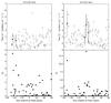 |
Fig. B.1 Upper (lower) panel: flux (TS) vs. time relative to tpeak for the symbiotic novae V1534 Sco (left) and V1535 Sco (right) in one-day bins. |
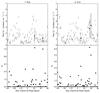 |
Fig. B.2 Upper (lower) panel: flux (TS) vs. time relative to tpeak for the recurrent novae T Pyx (left) and U Sco (right) in one-day bins. |
All Tables
List of novae in our catalog including the nova name, the coordinates, the optical peak time and apparent magnitude, t2 and the measured TS and flux in the sliding time window analysis.
All Figures
|
Fig. 1 Example optical light curves for 6 out of the 75 inspected novae. Observations reported by different telescopes and observers are shown in different colors. |
| In the text | |
|
Fig. 2 Duration of > 100 MeV gamma-ray emission as a function of t2 for the gamma-ray detected novae (candidates). |
| In the text | |
|
Fig. 3 Novae selected in a time range from August 2008 to the end of 2015. Left: spatial distribution in Galactic coordinates of the novae listed in Table A.1. Previously detected gamma-ray novae are shown in red. Right: optical peak apparent magnitude distribution of the novae, magnitudes of the five out of the six previously detected gamma-ray novae are overlaid in red. The peak magnitude of V959 Mon is not included because it has not been measured since the nova was too close to the Sun to be observed during its outburst. Most magnitudes are in V band. Peak magnitudes of novae that were only observed in I band are displayed by striped bars. |
| In the text | |
|
Fig. 4 Spectra from the six previously detected gamma-ray novae. The spectral energy distribution (SED) points including statistical uncertainties derived with the standard Galactic diffuse model are shown as black crosses, and a power law with exponential cutoff fit to that data is shown in blue. We show data points for bins with TS> 4, otherwise, we show 95% upper limits. The systematic uncertainties introduced by modeling the Galactic diffuse emission are estimated by repeating the analysis with alternative diffuse models. The envelope of the results using the alternative models are shown as gray bands for each energy bin. For V5668 Sgr, the fit did not constrain the cutoff energy, and we therefore present the results of a simple power-law fit. |
| In the text | |
|
Fig. 5 TS for sliding time windows of different length for the six known gamma-ray novae. The x-axis shows the time relative to the optical peak time tpeak. In the case of V959 Mon, the gamma-ray peak was used. |
| In the text | |
|
Fig. 6 Sketch of the sliding time window analysis. The start time of the time window is shifted in 2 day steps from 20 days before the peak time to 20 days after the peak time, i.e., the time window center moves from − 12.5 to 27.5 days relative to the peak time. |
| In the text | |
|
Fig. 7 Measured flux (TS> 4, shown in red) above 100 MeV and flux upper limits (shown in blue) for the various sliding time windows for the two novae V339 Del (left) and OGLE-2012-NOVA-01 (right). V339 Del is one of the previously known gamma-ray novae, while no gamma-ray emission was found for OGLE-2012-NOVA-01. |
| In the text | |
|
Fig. 8 Left: cumulative density of the TSmax distribution for the on-time (red) and off-time regions (blue) including only sources with TSmax< 25. Dotted (dashed) lines show the Gaussian equivalent one-sided 3σ (2σ) probability of finding a larger TS than the TS indicated by the intersection of the dashed line with the blue distribution. The dash-dotted line shows the 2σ probability after correction for trials. Right: sum of TS values for 69 novae. The value of the on-time data is shown as a red line, while the off-time data are shown in blue. The shaded blue band reflects the uncertainty introduced by the limited statistics of the off-time sample. |
| In the text | |
|
Fig. 9 Histogram of the time difference between the central time of the time window with maximum TS and the optical peak time (including all novae in our sample). The time difference can vary from − 12.5 to 27.5 days relative to the peak. Novae with a maximum TS smaller than 14.5 are shown in blue, sources with larger TS are plotted in red. |
| In the text | |
|
Fig. 10 Sliding time window results for V679 Car (left) and V1535 Sco (right). The upper row shows the TS value for each tested time window, while the lower row shows the measured flux above 100 MeV (TS> 4, red) or 95% flux upper limits (blue). |
| In the text | |
|
Fig. 11 TS map in the time window with maximum TS for V679 Car (left) and V1535 Sco (right). The white crosses indicate the point sources used in the model, i.e. the 3FGL background sources and the nova in the center. The black lines indicate the 3σ and 5σ contours. |
| In the text | |
|
Fig. 12 TS as a function of start and stop time in days relative to the peak time for V679 Car (left) and V1535 Sco (right). The maximum TS is marked with a black circle. |
| In the text | |
|
Fig. 13 Optical (bottom) and gamma-ray (top) light curves of V679 Car (left) and V1535 Sco (right). The gamma-ray data are binned in one-day bins. For days with TS< 4, we show 95% upper limits. |
| In the text | |
|
Fig. 14 SED for V679 Car (left) and V1535 Sco (right) using the duration obtained from Fig. 12. Both SEDs suffer from small statistics. The SED points derived with the standard Galactic diffuse model are shown as black crosses, and a power law with an exponential cutoff fit to these data is shown in blue. For V1535 Sco, the energy cutoff is not well constrained by the fit, and we therefore present the results of a simple power-law fit. The systematic uncertainties introduced by modeling the Galactic diffuse emission are estimated by repeating the analysis with alternative diffuse models. The envelopes of the results using the alternative models are shown as gray bands for each energy bin. |
| In the text | |
|
Fig. 15 Total emitted energy above 100 MeV as a function of the duration of the gamma-ray emission. Classical novae are marked with a circle and symbiotic novae with a triangle. The classical novae V679 Car is in agreement with the suggested relation between the total emission duration and the total energy of classical novae, while the symbiotic nova V1535 Sco emitted less energy than expected from the relation. |
| In the text | |
|
Fig. 16 Correlation of the gamma-ray flux with the optical peak apparent magnitude (left) and t2 (right): sources with TS> 14.5 (corresponding to 3σ) are shown as blue circles, while known gamma-ray novae are indicated as stars. Note that V959 Mon is not included because the peak was not covered by optical observations. Less significant sources are shown as upper limits indicated by arrows. The peak magnitude is measured in V band for most cases (shown in blue), but for a few cases, only I-band data were available (shown in green). |
| In the text | |
|
Fig. 17 Nova flux (blue) or flux upper limit (green) as a function of distance for a subsample of our catalog with estimated distances. Light green values indicate lower limits of the distance. |
| In the text | |
|
Fig. 18 Gamma-ray luminosity as a function of the optical peak apparent magnitude (left) and t2 (right). |
| In the text | |
|
Fig. 19 Sliding time window results for T Pyx extended to 60 days. The left panel shows the TS value for each tested time window, while the right panel shows the measured flux above 100 MeV (TS> 4, red) or 95% flux upper limits (blue). |
| In the text | |
|
Fig. 20 Upper (lower) panel: flux (TS) vs. time relative to tpeak for V745 Sco in one-day bins. No data are available from this position in the sky a few days before the peak because of a pointed observation of the LAT to observe M82. |
| In the text | |
|
Fig. 21 Measured distribution of the optical peak apparent magnitudes and best-fitting PLslope2 model. The Poissonian (1-σ) error bars are calculated with the method described by Gehrels (1986). |
| In the text | |
|
Fig. 22 Best-fitting gamma-ray flux: optical peak apparent magnitude distributions of several gamma-ray emissivity models (see text). The observed gamma-ray novae are overplotted for comparison. |
| In the text | |
|
Fig. B.1 Upper (lower) panel: flux (TS) vs. time relative to tpeak for the symbiotic novae V1534 Sco (left) and V1535 Sco (right) in one-day bins. |
| In the text | |
|
Fig. B.2 Upper (lower) panel: flux (TS) vs. time relative to tpeak for the recurrent novae T Pyx (left) and U Sco (right) in one-day bins. |
| In the text | |
Current usage metrics show cumulative count of Article Views (full-text article views including HTML views, PDF and ePub downloads, according to the available data) and Abstracts Views on Vision4Press platform.
Data correspond to usage on the plateform after 2015. The current usage metrics is available 48-96 hours after online publication and is updated daily on week days.
Initial download of the metrics may take a while.