| Issue |
A&A
Volume 609, January 2018
|
|
|---|---|---|
| Article Number | A80 | |
| Number of page(s) | 16 | |
| Section | Extragalactic astronomy | |
| DOI | https://doi.org/10.1051/0004-6361/201731048 | |
| Published online | 12 January 2018 | |
Jet-torus connection in radio galaxies
Relativistic hydrodynamics and synthetic emission
1 Institut für Theoretische Physik, Goethe Universität, Max-von-Laue-Str. 1, 60438 Frankfurt, Germany
e-mail: This email address is being protected from spambots. You need JavaScript enabled to view it.
2 Max-Planck-Institut für Radioastronomie, Auf dem Hügel 69, 53121 Bonn, Germany
3 Departament d’Astronomia i Astrofísica, Universitat de València, Dr. Moliner 50, 46100 Burjassot, València, Spain
4 Observatori Astronòmic, Parc Científic, Universitat de València, C/ Catedràtic José Beltrán 2, 46980 Paterna, València, Spain
5 Frankfurt Institute for Advanced Studies, Ruth-Moufang-Strasse 1, 60438 Frankfurt, Germany
Received: 26 April 2017
Accepted: 28 August 2017
Abstract
Context. High resolution very long baseline interferometry observations of active galactic nuclei have revealed asymmetric structures in the jets of radio galaxies. These asymmetric structures may be due to internal asymmetries in the jets or they may be induced by the different conditions in the surrounding ambient medium, including the obscuring torus, or a combination of the two.
Aims. In this paper we investigate the influence of the ambient medium, including the obscuring torus, on the observed properties of jets from radio galaxies.
Methods. We performed special-relativistic hydrodynamic (SRHD) simulations of over-pressured and pressure-matched jets using the special-relativistic hydrodynamics code Ratpenat, which is based on a second-order accurate finite-volume method and an approximate Riemann solver. Using a newly developed radiative transfer code to compute the electromagnetic radiation, we modelled several jets embedded in various ambient medium and torus configurations and subsequently computed the non-thermal emission produced by the jet and thermal absorption from the torus. To better compare the emission simulations with observations we produced synthetic radio maps, taking into account the properties of the observatory.
Results. The detailed analysis of our simulations shows that the observed properties such as core shift could be used to distinguish between over-pressured and pressure matched jets. In addition to the properties of the jets, insights into the extent and density of the obscuring torus can be obtained from analyses of the single-dish spectrum and spectral index maps.
Key words: galaxies: active / galaxies: jets / radiation mechanisms: non-thermal / radio continuum: galaxies
© ESO, 2018
1. Introduction
Active galactic nuclei (AGNs) are generally assumed to consist of a central, compact massive object (i.e. a supermassive black hole), an accretion disk surrounded by a molecular torus, and a jet launched perpendicular to the black-hole disk system. Within this standard model, AGNs may be classified according to their orientation with respect to the line of sight. If the AGN is seen at a viewing angle of ϑ = 90° (i.e. edge-on), the innermost regions are obscured by the torus and more internal features become observable as the viewing angle decreases (Antonucci 1993; Urry & Padovani 1995).
In addition to the classification of AGNs by their viewing angle, Fanaroff & Riley (1974) introduced a division based on the morphology of the jets: Fanaroff-Riley I (FR I) jets are characterised by a bright core and FR II jets are dominated by their bright lobes.
The large-scale structure of AGNs observed at high viewing angles can be resolved through radio interferometric observations (see e.g. Kharb et al. 2008) and high resolution very long baseline interferometry (VLBI) observations enable us to probe the morphological evolution of AGNs on parsec scales (see e.g. Lister et al. 2009). These jets remain collimated over long distances, up to kilo-parsec scales, at which they can be modelled using special-relativistic (magneto-)hydrodynamical [R(M)HD] simulations and the computed emission and polarisation properties provide insights into the underlying fluid properties and magnetic field configurations (see e.g. Perucho & Martí 2007; Laing & Bridle 2002; Hardcastle & Krause 2013).
In the infrared band, the electromagnetic emission from these AGNs is assumed to be generated by the re-emission by the obscuring torus of the radiation initially produced in the accretion disk. Based on observations, two kinds of torus models were constructed, namely smooth torus models and clumpy torus models (for a review of torus models, see e.g. Hoenig 2013).
So far both models have been applied successfully to explain observational results either at kilo-parsec scales (via jet simulations) or at sub-parsec scales (via torus simulations). However, to explain the VLBI observations of AGNs viewed almost edge-on  , jet and torus models need to be combined. In this paper we combine both approaches, addressing the question of the impact that the combination of the torus and the ambient medium have on the observed properties of the jet at parsec scales.
Additionally, we aim to make the connection between numerical simulations of relativistic outflows and their emission with observations in a deeper way than has been carried out so far. Jet acceleration, recollimation, and other phenomena have previously been analysed with the help of one-dimensional (1D), 2D, and 3D numerical simulations, including various characteristics such as magnetic fields and special relativity (see e.g. Mizuno et al. 2015). Some emission codes have even been applied (Gómez et al. 1997; Mimica et al. 2009) to explain the emission. Here we go one step further and consider additional components in the AGN picture, such as the obscuring torus, and including time delays, emission and absorption in a code, which will enable us to compare with real observations of two-sided sources in future works.
The organisation of the paper is as follows. In Sect. 2 we introduce our numerical set-up for the jet and torus. The results of the simulations and emission calculations are presented in Sects. 3.1 and 3.2. The discussion of our results is provided in Sect. 4. Throughout the paper we assume an ideal-fluid equation of state  , where p is the pressure, ρ the rest-mass density, ϵ the specific internal energy, and
  the adiabatic index (Rezzolla & Zanotti 2013).
2. Special-relativistic hydrodynamic simulations
We performed several 2D axisymmetric simulations of supersonic special-relativistic hydrodynamical jets via the finite-volume code Ratpenat (for more details see Perucho et al. 2010, and references therein).
2.1. Jet model
The numerical set-up is similar to that used in Fromm et al. (2016) and for completeness we provide below a short summary.
The numerical grid consisted of 320 cells in the radial direction and 400 cells in the axial direction. Using a numerical resolution of 4 cells per jet radius1 (Rj), the grid covered 80 Rj × 100 Rj. We assumed the z axis to be in the direction of propagation of the jet and x-axis to represent the radial cylindrical coordinate.
We used outflow conditions at z = zmax and R = Rmax and, owing to the axisymmetry, we applied reflection conditions at R = 0. At z = 0 we used inflow conditions for r ≤ 1 Rj, i.e. we injected a velocity vb parallel to the z-axis and outflow conditions for R>Rj. We initialised a pre-existing jet along the simulation box surrounded by a dense ambient medium with decreasing pressure gradient. The jet is characterised by the following parameters at injection (z = 0): the velocity of the jet vb, the classical Mach number of the jet M, the rest-mass density of the jet ρb, and the adiabatic index  . The bulk Lorentz factor Γ was computed from the jet velocity and pressure, pb at the jet nozzle from the Mach number using an ideal-fluid equation of state. The ratio dk = pb/pa between the pressure in the jet, pb, and the pressure in the ambient medium, pa, led to either a pressure matched (PM) jet (i.e. with dk = 1) or to an over-pressured (OP) jet (i.e. with dk> 1).
Depending on this ratio, internal structures in the jet, the so-called recollimation shocks were formed in the case of an OP jet or, in the case of a PM jet, the jet appeared featureless (Mizuno et al. 2015). The properties of the ambient medium (e.g. the gradient in the ambient pressure and ambient rest-mass density) played a crucial role in the shape of the jet and the properties of the created recollimation shocks in the case of OP jets. We modelled the decrease in the ambient medium pressure with a pressure profile presented in Gómez et al. (1997) as ![Mathematical equation: \begin{equation} p_{\rm a}(z)=\frac{p_{\rm b}}{d_{\rm k}}\left[1+ \left(\frac{z}{z_{\rm c}}\right)^n\right]^{-\frac{m}{n}}, \label{pamb} \end{equation}](/articles/aa/full_html/2018/01/aa31048-17/aa31048-17-eq29.png) (1)where zc can be considered as the core radius and the exponents n and m control the steepening of the ambient pressure. The initial conditions, given in code units, where speed of light c = 1, jet radius is Rj, and ambient medium rest-mass density, ρa = 1 g cm-3, are listed in Table 1.
(1)where zc can be considered as the core radius and the exponents n and m control the steepening of the ambient pressure. The initial conditions, given in code units, where speed of light c = 1, jet radius is Rj, and ambient medium rest-mass density, ρa = 1 g cm-3, are listed in Table 1.
 |
Fig. 1 Distribution of ambient pressure and ambient rest-mass density in code units for the gradients in the ambient medium. |
Initial parameters for the jet.
The distributions of the ambient pressure and ambient rest-mass density for the parameters for the jet models considered here are shown in Fig. 1. The external pressure gradient is kept constant during the simulation by adding an external force, which preserves the pressure gradient without affecting the dynamics of the jet (see also Gómez et al. 1997). Throughout the paper we used a single value of n = 1.5, while setting m = 2, 3, 4 and excluding gravity and cooling processes during the SRHD simulations.
2.2. Torus model
Once a stationary state for the jet was reached, typically after five grid longitudinal crossing times, we inserted a steady-state torus. The included torus acts only as an absorber for the synchrotron radiation generated in the jet and has no influence on the dynamics of the jet. Therefore the torus should be regarded as a phenomenological model; Stalevski et al. (2016) provide a detailed discussion of the torus modelling.
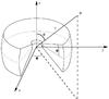 |
Fig. 2 Geometry of the assumed torus model (adapted from Stalevski et al. 2012). |
More specifically, our torus model is adapted from Stalevski et al. (2012, 2016) and the geometry of the torus can be seen in Fig. 2. The geometry of the model resembles a flared disk and is characterised by three parameters: the inner radius of the torus, Rin, outer radius of the torus, Rout, and the half-opening angle Θ. For the inner radius of the torus we used 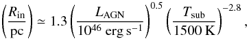 (2)where LAGN is the bolometric luminosity and Tsub is the sublimation temperature of the dust grains. We assumed a power law distribution for the rest-mass density in the torus, given by
 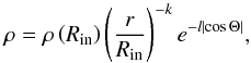 (3)where the cosΘ-dependence in the Eq. (3) leads to a concentration of rest-mass density towards the equatorial plane. Since we did not perform a radiative modelling of the torus, its temperature distribution is simply assumed to follow a certain prescription. In particular, following Schartmann et al. (2005), the temperature decrease moving outward in the radial direction; furthermore, because of the direct illumination of the inner torus walls, the temperature should decrease when going from high to low latitudes. Such behaviour may be modelled with the following temperature profile
 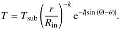 (4)Figure 3 illustrates the distribution of the temperature and rest-mass density in the torus with LAGN = 1043 erg s-1, Tsub = 1500 K, which leads to an inner radius of Rin = 4 Rj. The outer radius is set to Rout = 30 Rj and the angular thickness of the torus is θ = 50°. For the scaling of the rest-mass density we set
  , while the exponents for the distribution of the temperature and rest-mass density are k = 1 and l = 2.
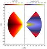 |
Fig. 3 Left panel: distribution of temperature in the meridional plane. Right panel: corresponding rest-mass density distribution. The Θ-dependence in the distribution of the temperature and the rest-mass density is clearly visible. |
 |
Fig. 4 Example of the 3D geometry of the jet-torus model. |
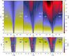 |
Fig. 5 Stationary results for the jet simulations. The panels show the 2D distribution of the rest-mass density for different ambient medium configurations as indicated by the exponent m. In each panel the left side (−30 <r/Rj< 0) corresponds to the OP jet and the right side (0 <y/Rj< 30) to the PM jet. The top row spans the entire simulation grid whereas the bottom row shows a magnified view of the nozzle region (−7 <z/Rj< 7). The white lines in the bottom row show stream lines visualising the direction of the flow and the bold dashed lines correspond to the inward travelling and reflected shock wave. |
The combined system consisting of jet, counter-jet, and torus is shown in Fig. 4. The observed image is the projection of the jet-torus system onto the x−y plane. In Fig. 4 a distant observer would see the jet-torus system at a viewing angle of ϑ = 0°.
3. Results
3.1. Special-relativistic hydrodynamics
In Fig. 5 we show the 2D distribution of the rest-mass density of the stationary jets from our (SRHD) simulations. Each panel corresponds to a different ambient medium configuration as characterised by the exponent m (see Eq. (1)). The left half of each panel (−30 <r/Rj< 0) shows the distribution for the OP jet and the right half of each panel (0 <r/Rj< 30) for the PM jet. The top row presents the entire simulation grid and the bottom row gives a magnified view of the nozzle region of the jets (0 <z/Rj< 7).
In the case of OP jets, the initial pressure mismatch at the nozzle led to the generation of two shock waves: one travelling radially outward and the other propagating inward in the direction of the jet axis. Between these two shocks the jet radially expanded until a pressure equilibrium with the ambient medium was reached. This equilibrium is first obtained at the jet-ambient medium boundary and leads to an inward travelling wave, which is indicated by the bold dashed lines in the bottom row of Fig. 5. The radial expansion of the jet is stopped as soon as the expansion regions are crossed by the inward travelling sound waves. Since these waves propagate with the local sound speed, the outer regions in the jet already stop expanding while the inner regions continue to expand (further decreasing the pressure and rest-mass density). The innermost region in the jet stops expanding as soon as the sound wave reaches the jet axis. At this position, a recollimation shock is formed, which can be regarded as a new jet nozzle (local maximum in pressure and rest-mass density) and so the flow expands again (see e.g. Daly & Marscher 1988; Falle 1991; Mizuno et al. 2015). The recollimation shocks are clearly visible at z ~ 6 Rj in the top half of the panels in the left column of Fig. 5. At the position of the recollimation shock, a new radially outward travelling wave is formed and the jet expands again.
If the pressure gradient in the ambient medium at the position of the first recollimation shock (z ~ 6 Rj) is steep enough, the sound waves reflected from the boundary between the jet and ambient medium (generated after reaching radial pressure equilibrium) cannot reach the jet axis and therefore no additional recollimation shock is formed and the jet continues to expand (for detailed discussion see Porth & Komissarov 2015). With our settings for the ambient medium, this behaviour was obtained for the models with m> 2. In these cases, even for the OP jets no additional recollimation shocks were formed beyond zc ~ 6 Rj and a conical jet shape was obtained further downstream.
In contrast to the OP jets, in PM jets there is a radial-pressure equilibrium at the nozzle. Therefore, only minor variations are created within the jet and the pressure and rest-mass density are continuously decreasing. If the pressure in the jet decreases faster than the pressure in the ambient medium, there is a position along the jet at which the pressure in the ambient is higher than in the jet. At this position a re-confinement shock is created that is travelling towards the jet axis (Komissarov & Falle 1997). This behaviour can be seen in case of PM jets embedded in an ambient medium with pressure gradient m = 4 at z ~ 60 Rj in Figs. 5 and 6. The opening angle of these jets depends on the gradient in the ambient medium: the steeper the gradient the larger the opening angle of the jet. This behaviour is visible in the first column of Fig. 5.
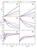 |
Fig. 7 Variation of the jet parameters along the jet axis. The left column corresponds to OP jets and the right column to PM jets. From top to bottom: the jet radius, axial pressure, and axial velocity in the z-direction are shown (see text for details). |
A detailed picture of the influence of the pressure ratio at the jet nozzle, dk, and the configuration of the ambient medium on the shape of the jet and its fluid parameters can be obtained by analysing their evolution along the jet axis. The variation of the normalised jet radius, r/Rj, of the axial pressure, paxial, and of the axial velocity, vaxial, for the different jet and ambient medium models is shown in Fig. 7. The largest variations in the jet parameters occur at small scales (i.e. for z ≲ 20 Rj) and for different jet models, i.e. pressure matched or over-pressured. Within a jet model the modification of the gradient in the ambient medium leads to variations, but does not lead to a different evolution of the parameters along the jet axis.
In the case of PM jets, stronger gradients in the ambient medium lead to larger jet radii, r, faster velocities, vaxial, and smaller axial pressures, paxial. This behaviour can be understood in the following way: the radial position where a pressure equilibrium between the jet and the ambient medium is reached (given the same initial pressure at the jet nozzle) shifts downstream with the gradient in the ambient medium. Since the jet is in pressure equilibrium with the ambient medium, the axial pressure in the jet is equal to the pressure in the ambient medium, so that the steeper the gradient in the ambient medium the stronger the decrease in the jet pressure. According to the conservation equations of hydrodynamics, a hot supersonic flow accelerates if its cross section increases (Rezzolla & Zanotti 2013); thus a PM jet that is embedded in an ambient medium with larger gradients (hence larger jet radii) develops higher velocities than the same jet that is surrounded by an ambient medium with smaller gradients (see bottom panel of Fig. 7).
In contrast to the smooth evolution of the jet parameters (r, paxial, and vz,axial) for the PM jet, large variations are present in the parameters for OP jets (see Fig. 7). As already mentioned the initial pressure mismatch at the jet nozzle led to an opening of the jet and as soon as a radial pressure equilibrium was reached a radially inward travelling wave was formed. The larger the gradient in the ambient medium, the larger the jet radii where the pressure equilibrium was obtained became. Because of the finite sound speed, the crossing time of this wave increased with jet radius. The inner parts of the jet stopped expanding as soon as the sound wave crossed the jet axis. Therefore, the pressure decreased for larger jet radii, i.e. a steeper gradient in the ambient medium (compare solid red and blue lines in the middle panel of Fig. 7).
After the sound wave crossed the jet axis, the pressure increases to values comparable with the pressure in the ambient medium (see middle panel of Fig. 7 at z ~ 8 Rj). The difference in position of the pressure jump and its magnitude reflects the difference in the sound crossing time and the gradient in the ambient medium. Since the OP jets exhibit larger jet radii than PM jets, the fluid was accelerated to higher velocities, vz,axial at z ~ 5 Rj. The formation of the recollimation shock at z ~ 6 Rj leads to a sharp decrease in the axial velocity vz,axial, and the expansion of the fluid after crossing the recollimation shock leads to an increase in the axial velocity. After z> 10 Rj, the rapid decrease in the ambient-medium pressure induces an expansion of the jet, which is accompanied by a decrease in the jet pressure, paxial, and a slight increase in the axial jet velocity. In the case of the smallest gradients in the ambient medium (m = 2) additional recollimation shocks are formed at z ~ 20 and at z ~ 40 (see the solid red curve in Fig. 7).
3.2. Emission
For the calculation of the emission we followed the methods described in Gómez et al. (1997) and Mimica et al. (2009). For completeness we provide here the basic equations and underlying assumptions for the calculation of non-thermal emission. We assumed a power law distribution of relativistic electrons and included adiabatic, but neglected synchrotron cooling during the calculation of the non-thermal emission. Since the magnetic fields used in the computation of the emission were well below the equipartition ratio (ϵb< 0.2), we expected no or only a minor influence of radiative cooling on the non-thermal emission in the radio regime  ,
,  (5)where n0 is a normalisation coefficient, γ is the electron Lorentz factor, γmin and γmax are the lower and upper electron Lorentz factors and s is the spectral slope. In order to construct the distribution of non-thermal particles from the thermal population we assumed that the number density of relativistic particles is a fraction ζe of the thermal particles
  (6)where mp is the proton mass. The second assumption relates the energy in the relativistic particles to the energy in the thermal particles via the parameter ϵe as follows:
  (7)where me is the electron mass. After performing the integration in Eqs. (6) and (7) a relation for lower electron Lorentz factor, γe, min, may be derived as
 ![Mathematical equation: \begin{equation} \gamma_{\rm e,\,min}=\left\{ \begin{array}{ll} \displaystyle \frac{p}{\rho} \frac{m_{\rm p}}{m_{\rm e} c^2}\frac{(s-2)}{(s-1)(\hat{\gamma}-1)}\frac{\epsilon_{\rm e}}{\zeta_{\rm e}} & \textrm{if }s>2 , \\ \displaystyle \left[\frac{p}{\rho} \frac{m_{\rm p}}{m_{\rm e} c^2}\frac{(2-s)}{(s-1)(\hat{\gamma}-1)}\frac{\epsilon_{\rm e}}{\zeta_{\rm e}} \gamma_{\rm e,\,max}^{s-2}\right]^{1/(s-1)} & \textrm{if }1<s<2 , \\ \displaystyle \frac{p}{\rho}\frac{\epsilon_{\rm e}}{\zeta_{\rm e}} \frac{m_{\rm p}}{m_{\rm e} c^2(\hat{\gamma}-1)} \left[ \ln\left(\frac{\gamma_{\rm e,\,max}}{\gamma_{\rm e,\,min}}\right) \right]^{-1} & \textrm{if } s=2 . \label{gmineq1} \end{array}\right. \end{equation}](/articles/aa/full_html/2018/01/aa31048-17/aa31048-17-eq103.png) (8)For the upper electron Lorentz factor we used a constant ratio of the lower electron Lorentz factor, namely
(8)For the upper electron Lorentz factor we used a constant ratio of the lower electron Lorentz factor, namely  (9)The normalisation coefficient of the non-thermal particle distribution can be obtained by performing the integral in Eq. (6) within the boundaries given by γe, min and γe, max, yielding
 ![Mathematical equation: \begin{equation} n_0=\frac{\epsilon_{\rm e} p (s-2)}{\left(\hat{\gamma}-1 \right)\gamma_{\rm e,\,min}^2 m_{\rm e} c^2}\left[ 1-\left(\frac{\gamma_{\rm e,\, max}}{\gamma_{\rm e,\,min}}\right)^{2-s}\right]^{-1} \cdot \end{equation}](/articles/aa/full_html/2018/01/aa31048-17/aa31048-17-eq106.png) (10)Since the information on the magnetic field cannot be obtained from our purely hydrodynamical numerical simulations, we introduced it through its fraction ϵB of the equipartition magnetic field, namely, we set
(10)Since the information on the magnetic field cannot be obtained from our purely hydrodynamical numerical simulations, we introduced it through its fraction ϵB of the equipartition magnetic field, namely, we set  (11)Following Mimica et al. (2009), the emission and absorption coefficients for the non-thermal emission, respectively ϵν,nt and αν,nt, may be written as2
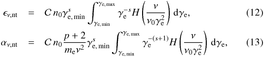 where the characteristic frequency, ν0 = 3eBsinθ/ (4πmec) with θ the angle between the direction to the observer and the direction of the magnetic field,
  , and e is the electron charge.
The value of H(ξ) depends on the orientation of the magnetic field. If the magnetic field is ordered, H(ξ) = F(ξ), i.e.  (14)where K5/3 is the modified Bessel function of the second kind of order 5/3; in the case of a random magnetic field H(ξ) = R(ξ), so that
  (15)with α the angle between the comoving magnetic field and the line of sight. For the functions F(ξ) and R(ξ) we used the approximations given by Crusius & Schlickeiser (1986) and Joshi & Böttcher (2011), namely
 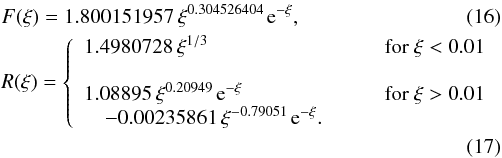 In order to compute the observed emission, we transformed the coefficients of emission ϵν,nt and absorption αν,nt, into the observer’s frame and corrected for cosmological effects
  where the Doppler factor is defined as D: = Γ-1(1−vbcosϑ)-1 and z denotes the redshift.
In addition to the non-thermal component, the emission also includes the contribution from a dusty torus, such that the thermal absorption coefficient αν,th is given by  (20)where Z = μi/μe, with μe = 2/(1 + X); and μi = 4/(1 + 3X), where X corresponds to the abundance of hydrogen (set here to be X = 0.71); and
  is the velocity-averaged gaunt factor (see e.g. Rybicki & Lightman 1986). For the gaunt factor we used the values tabulated by van Hoof et al. (2014) and applied a bi-linear interpolation in log u – log γ2 space, where u = (hν)/(kbT) and γ2 = (Z2Ry)/(kbT), and Ry is the Rydberg energy.
The total intensity, Iν, was a mixture of the non-thermal emission/absorption and thermal absorption (if the ray propagated through the dusty torus) and was computed via the transport equation as  (21)where ds is the path length along a ray. For the calculation of the emission we computed the starting point of each ray at the position where the optical depth τ = τlimit and followed the ray to the observer. We used a passive tracer advected during the SRHD simulations to distinguish between ambient medium (tracer = 0), jet (tracer ≈ 1) and torus (tracer = 2). The optical depth is defined as
  (22)The observed flux density can be computed from the intensity according to
  (23)where DL is the luminosity distance and Δx and Δy represent the resolution of the detector’s frame. The luminosity distance is computed via the equation provided by Pen (1999), where we took Ωm = 0.27 and a Hubble constant of H0 = 71 km s-1 Mpc-1. The final jet-torus geometry at a viewing angle of ϑ = 0° used for the calculation of the emission is shown in Fig. 4; furthermore, hereafter we assumed (DL = 21.1 Mpc), which corresponds to a redshift of z = 0.005.
3.3. Parameter space study
In this section we analyse the influence of the emission and torus parameters on the observed spectrum. In Table 2 we provide an overview of the parameters used and of the values for our reference model. Generically, such parameters can be divided into three classes: i) scaling parameters; ii) emission parameters; and iii) torus parameters; we discuss these separately below.
Parameters for the emission simulations and values for the reference model.
In order to cover a wide frequency range, i.e. 109 Hz <ν< 1012 Hz, we used a logarithmic grid with 100 frequency bins. The ray tracing was performed with a Delaunay triangulation on the axisymmetric RHD simulations with (r,z) coordinates to a 3D Cartesian grid (x,y,z) with a typical resolution of 3003 cells (see Fig. 4 for a 3D representation of the jet-torus system).
3.3.1. Single-dish spectra
To demonstrate the influence of the torus on the spectrum, we computed the emission for the reference model with and without a torus. The result of these calculations is presented in Fig. 8, where the black lines indicate simulations including a torus, while red lines are used for simulations without a torus. Furthermore, solid lines refer to the total flux density, while dashed and dotted lines correspond to the emission from the jet and counter-jet, respectively.
Not surprisingly, in the low-frequency regime, i.e. for ν < 1011 Hz, simulations with a torus show a smaller flux than simulations without a torus, simply as a result of the increased absorption along the line of sight. At higher frequencies, the flux densities of both simulations are very similar since the torus becomes optically thin at these frequencies. The comparison between the emission from the jet (dashed lines) and counter-jet (dotted lines) shows that the counter-jet is more affected by the absorption of the torus than the jet. Similar to the case of the total flux density, the emission from jet and counter-jet including a torus converges to their counter parts without torus (at ν ~ 1011 Hz for the jet and at ν ~ 3 × 10¹¹ Hz for the counter-jet).
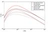 |
Fig. 8 Single-dish spectra for a simulation including a torus (black) and without a torus (red). |
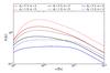 |
Fig. 9 Single-dish spectra for the different jet and ambient medium models. |
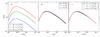 |
Fig. 10 Influence of the scaling parameters Rj, ϑ, and Lkin on the shape of the observed single-dish spectrum. |
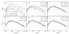 |
Fig. 11 Influence of the emission parameters ρa,ϵe,ϵb,ζe,ϵγ, and s on the shape of the observed single-dish spectrum. |
Figure 9 shows the single-dish spectrum for the different jet-torus and ambient medium models (see Table 1). Within the same ambient medium, the PM jets (dk = 1; dashed lines in Fig. 9) exhibit higher flux densities than the OP jets (dk = 2.5, solid lines in Fig. 9). Furthermore, OP jets show a flatter spectrum than PM jets within 109 Hz ≤ ν ≤ 1011 Hz. The general trend could be described as follows: the steeper the gradient in the ambient medium, the flatter the spectrum. The change in the spectral slope at ν ~ 1011 Hz is indicative of the turnover frequency of the torus, i.e. the frequency at which the torus becomes optically thin (see also Fig. 8).
Figure 10 is meant to summarise the impact of the different scaling parameters, Rj,ϑ, and,Lkin, on the single-dish spectrum. More specifically, we computed the emission when only one of the scaling parameters is varied while the others are kept fixed to the values listed in Table 2. The variation in the observed flux can then be summarised as follows:
-
Jet radius, Rj: the jet radius acts as the scaling length of thesimulations and has the largest impact on the observedsingle-dish spectrum (see panel a in Fig. 10). Theincrease in flux with Rj follows a simple scaling
 , as expected from Eq. (23).
 -
Viewing angle, ϑ: owing to Doppler boosting, the observed spectrum is shifted towards higher flux densities and higher turnover frequencies with decreasing viewing angle. Since we use large viewing angles for our simulations the variations in the spectrum are minor.
-
Bolometric luminosity, Lkin: changes in the bolometric luminosity lead to a variation in the inner radius of the torus (cf. Eq. (2)). Lowering the kinetic luminosity decreases the inner radius of the torus. Since we keep the outer radius of the torus fixed, the total size of the torus increases with decreasing kinetic luminosity and lower values for rest-mass density and temperature are obtained. Since the opacity of the torus scales as τtorus ∝ T− 1/2ρ2 (when assuming T and ρ to decay as r− k), lower densities lead to lower opacities and a large emission from the jet. As a result, the observed flux density increases with decreasing kinetic luminosity.
In Fig. 11 we report the effect of the emission parameters ϵe,ϵb,ζe,ϵγ, and s on the observed single-dish spectrum while keeping the other parameters fixed. The emission simulations were performed using our reference model (see Table 2).
-
Ambient medium rest-mass density, ρa: a variation in the ambientmedium rest-mass densityρa leads to large changes in the shape and total flux density of the spectrum (see panel a in Fig. 11). The single-dish spectrum steepens and is shifted to higher turnover flux densities with increasing ambient medium rest-mass density.
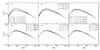
Fig. 12 Influence of the torus parameter on the observed single-dish spectrum. Top row from left to right: the torus outer radius, torus thickness, and torus rest-mass density are shown. Bottom row from left to right: the torus temperature, distribution of the torus rest-mass density, and distribution of the torus temperature are shown.
-
Thermal to non-thermal energy ratio,ϵe: if more energy is stored in the non-thermal particles via an increase in ϵe, the turnover frequency increases, while the turnover flux density rises only slightly. The spectral index within ν ~ 1011 Hz decreases in absolute values, thus leading to a flatter spectrum (see panel b in Fig. 11).
-
Equipartition ratio, ϵb: an increase of the equipartition ratio ϵb leads to higher observed flux densities on the single-dish spectrum and to a shift of the turnover position towards lower frequencies and higher flux densities (see panel c of Fig. 11). Additionally, the spectrum steepens for ν< 1011 Hz.
-
Ratio between thermal to non-thermal number densities, ζe: increasing the number of non-thermal particles leads to higher observed flux densities and shifted the turnover frequency towards lower frequencies. Additionally, the spectral slope increases (see panel d of Fig. 11).
-
Ratio between upper and lower e−-Lorentz factors, ϵγ: the variation of ϵγ had only a minor effect on the single-dish spectrum (see panel e in Fig. 11). An increase in γmax leads to a flattening of the spectrum at high frequencies (ν > 1011 Hz) and shifted the high-frequency cut-off in the spectrum towards higher frequencies, which are clearly visible for γe = 102 (see blue line in panel e).
-
Spectral slope, s: changing the spectral slope of the non-thermal particle distribution induced only minor variations in the observed flux densities. However, the slope of the spectrum for ν ≤ 1011 Hz flattens, while for ν > 1011 Hz the spectral slope steepens with increasing s (see panel f in Fig. 11).
Since the properties of the obscuring torus strongly affect the observed emission, we also performed a parameter-space study varying the properties of the torus reported in Table 2. In our model the torus is characterised by its geometry (Rout and Θ) and by the distribution of the rest-mass density and temperature (see Eqs. (3), (4)). The first row in Fig. 12 summarises the changes in the single-dish spectrum that result from the torus geometry, while the second row shows the modification in the spectral shape depending on the distribution of the rest-mass density and temperature. Overall, the variations in the spectrum can be summarised as
-
Torus geometry: the variation of the torus geometry and its effecton the single-dish spectrum is presented in the top row ofFig. 12. From left to right we show the effects of thetorus outer radius, Rout, the torus thickness, Θ, and the torus rest-mass density, ρt. Increasing the outer radius of the torus leads to a drop in the observed emission between 109 Hz ≤ ν ≤ 1011 Hz. The influence of the torus thickness is presented in panel b of Fig. 12, which shows that the observed flux density decreases as the thickness of the torus is increased.
-
Density distribution: the observed flux density decreases with increasing torus rest-mass density. At the same time, the turnover frequency is shifted towards higher frequencies (see panel d in Fig. 12).
-
Temperature distribution: variations in the temperature of the torus only have minor impacts on the observed flux density, so that the hotter the torus the higher the observed flux density (see panel g in Fig. 12).
-
Radial and angular distribution of the torus rest-mass density and torus temperature: the gradient in the radial direction mainly modifies the total observed flux density with a steeper gradient in the radial direction leading to an increase in the flux density (see panel e in Fig. 12). On the other hand, a larger effect on the shape of the spectrum comes from changing the gradient in the polar direction (see panel f). More specifically, if the temperature distribution is more concentrated at the edges and the rest-mass density falls off more rapidly towards the edges of the torus (i.e. if higher values for l are used), the spectrum steepens and the observed flux density is higher than for smoother rest-mass density and temperature distributions (i.e. for lower values for l).
All things considered, the parameter study on the single-dish spectrum can be summarised as follows: the scaling parameter Rj and the ambient medium rest-mass density ρa have the largest impact on the observed single-dish flux density (see panel a in Figs. 10 and 11). Changes in the emission parameters, ϵe,ϵb,ζe,ϵγ, and s mainly modify the shape of the spectrum and lead only to minor variations in the flux density (see Fig. 11). The torus parameters show the smallest effect and mainly alter the slope in the optically thin regime of the spectrum (see Fig. 12).
VLBA properties used for the convolution of the radio maps.
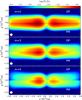 |
Fig. 13 Convolved radio maps at 15 GHz. In each panel the range from −3 × 1018 cm <x< 0 cm indicates the jet (pointing towards the observer) and the range from 0 mas <x< 3 × 1018 cm corresponds to the counter-jet. The panels correspond to different gradients used in the ambient medium indicated by n and m. In each panel the the top half corresponds to an OP jet and the bottom half to a PM jet. The convolving beam is plotted in bottom left corner of each panel. |
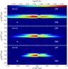 |
Fig. 14 Same as Fig. 13 at a frequency of 86 GHz. In each panel the range from −1.5 × 1018 cm <x< 0 cm indicates the jet (pointing towards the observer) and the range from 0 mas <x< 1.5 × 1018 cm corresponds to the counter-jet. The panels correspond to different gradients used in the ambient medium indicated by n and m. In each panel the top half corresponds to an OP jet and the bottom half to a PM jet. The convolving beam is plotted in the bottom left corner of each panel. |
3.3.2. Synthetic radio maps
To facilitate comparison with VLBI observations, we computed radio maps at different frequencies and convolved these frequencies with a 2D Gaussian beam. The size of the beam depends on the properties of the array and on the observing frequency. In Table 3 we present the typical beam sizes (uniform weighting, full-track (u,v) coverage for a source at −8° declination) for the Very Long Baseline Array (VLBA) and its sensitivity, i.e. the lowest detectable thermal noise (see the EVN calculator3, for details). If not stated otherwise, a flux-density cut-off of 5 × Slimit was used for the synthetic radio maps.
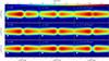 |
Fig. 15 Influence of the viewing angle (left column), the thermal to non-thermal energy ratio (middle column) and the torus rest-mass density (right column) on the 15 GHz radio maps. In each panel the range from −3 × 1018 cm <x< 0 cm indicates the jet (pointing towards the observer) and the range from 0 mas <x< 3 × 1018 cm corresponds to the counter-jet. The convolving beam is plotted in the bottom left corner of each panel. |
In Fig. 13 we show the convolved radio maps at 15 GHz for different ambient medium and jet models (similar to Fig. 5). The panels show, from top to bottom, various models for the ambient medium and in each panel the top half, i.e. (0–1) × 1018 cm corresponds to the OP jet, and bottom half, i.e. (− 1−0) × 1018 cm, to the PM jet. The width of the jet increases with the gradient in the ambient medium, from top to bottom, from 0.5 × 1018 cm to 0.8 × 1018 cm, while the observed flux density decreases. Within a common atmosphere, the OP jets (top half of each panel) show a less elongated core region as compared to the PM jets (bottom half of each panel) and the axial flux density decreases faster in OP jets than in PM jets. These effects become more visible as the rest-mass density gradient in the ambient medium is increased.
Analogous to the parameter study performed on the single-dish spectra (see Sect. 3.3.1), we investigated the impact of the emission parameters presented in Table 2 on the synthetic radio maps. Figure 15 summarises the effects of the viewing angle, ϑ, the thermal to non-thermal energy ratio ϵe, and the rest-mass density of the torus, ρt, on the 15 GHz radio maps. For a better comparison, the reference model is included in the second row of Fig. 15.
At smaller viewing angles (i.e. for ϑ = 60°), the jets appear more asymmetric because of the increased Doppler boosting and larger opacity along the line of sight, especially for the counter-jet (see the top panel in the first row of Fig. 15). However, with increasing viewing angle the asymmetries between jet and counter-jet tend to disappear, while the total flux density in the radio map decreases. Upon varying the non-thermal to thermal energy ratio ϵe, the flux density increases and affects both jets in the same way (see second row in Fig. 15). On the other hand, a change in ϵe does not alter the jet structure or the emission gap between the jet and counter-jet.
In the third row of Fig. 15 we show the changes in the 15 GHz radio maps due to a variation in the torus rest-mass density, ρt. Since we keep the torus size constant, a change in the torus rest-mass density does not have an impact on the observed emission at |x| > 1 × 1018 cm. However, the observed gap between jet and counter-jet does change depending on the torus rest-mass density. In particular, the gap is nearly invisible at low densities (top panel in the third row) while it is clearly noticeable at higher densities (see last panel in the third row of Fig. 15). Besides the changes in the gap between the jet and counter-jet, a variation in the torus rest-mass densities leads to changes in the observed flux densities within |x| < 1 × 1018 cm. This can be easily explained as due to the increased opacity, which reduces the flux reaching the observer (see the decreasing flux density at x = 0.5 × 1018 cm).
In the analysis of VLBI observations it is common to compute spectral index maps, where the spectral index, α, between to adjacent frequencies ν1 and ν2 is given by  (24)To avoid resolution-induced artefacts in the spectral index maps, a common beam size was used for the convolution. Furthermore, as usual in observational VLBI to avoid over-resolution from the high-frequency image, the beam size was set on the low-frequency map.
In Fig. 16 we present the spectral index computed between 22 GHz and 43 GHz for different torus densities indicated in the top left corner. The spectral index (SPIX) is found to be negative (i.e. α ~ −0.6) for regions | x | > 0.5 × 1018 cm to reflect optically thin regions, and positive (i.e. α ~ 2.5) for | x | < 0.5 × 1018 cm to reflect optically thick jet regions.
These inner regions absorb a large amount of the emission because of the high rest-mass density in the surrounding torus. Indeed, as the torus rest-mass density is increased, more emission is found to be absorbed and the optically thick region expands towards the edges of the torus (compare the top to the bottom panels in Fig. 16). Besides the expansion of the optically thick region, the spectral index also generally increases for larger torus rest-mass densities. Thus, the extent of the optically thick region and the value of the spectral index can be used to deduce the size and rest-mass density of the obscuring torus.
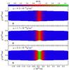 |
Fig. 16 Spectral index maps computed between 22 GHz and 43 GHz for various torus densities. In each panel the range from −3 × 1018 cm < x < 0 cm indicates the jet (pointing towards the observer) and the range from 0 mas < x < 3 × 1018 cm corresponds to the counter-jet. The convolving beam is plotted in the bottom left corner of each panel. |
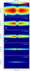 |
Fig. 17 Synthetic multi-frequency radio maps from 8 GHz to 86 GHz. In each panel the range from −3 × 1018 cm < x < 0 cm indicates the jet (pointing towards the observer) and the range from 0 mas < x < 3 × 1018 cm corresponds to the counter-jet. The convolving beam is plotted in the bottom left corner of each panel. |
Multi-frequency VLBI observations enabled us to investigate the opacity and therefore the frequency-dependent position of the so-called “radio core”, i.e. of the first detectable flux-density maximum. The variation of this position with frequency provides details of the rest-mass density and the magnetic field in the source. This effect is called core shift (see Lobanov 1998, for details). In VLBI observations the initial position of the jet is lost during the imaging process, and various techniques are used to reconstruct the core shift between adjacent frequencies (see Fromm et al. 2013, for a summary). However, this is not needed when working with synthetic radio maps, since the initial position is known. Here, we defined the core as the position of the first flux-density maximum along an axial slice through the convolved radio map.
In Fig. 17 we present multi-frequency VLBI radio maps from 8 GHz to 86 GHz based on our reference model (see Table 2 for the parameters used). The total flux density of the radio maps and the transversal size of the jets decreased with frequency, where the latter could be explained by the convolution with the observing beam (see Table 3). Given the parameters used for our reference model, the turnover frequency is at ~ 8 GHz, so that the flux density decreases as Sν ∝ ν− (s−1)/2 for ν> 8 GHz. Since the flux density is lower at higher frequencies and the sensitivity of the array also decreases with frequency (see third column of Table 3), the jets appear shorter in size at higher frequencies. Furthermore, besides a drop in the observed emission with frequency, the gap between the jet and counter-jet is reduced with frequency and the position of the flux-density maximum in the jet and the counter-jet is shifted upstream.
In Fig. 18 we present the core shift obtained from the synthetic multi-frequency radio maps shown in Fig. 17. The red stars correspond to the position of the radio core in the counter-jet and the blue stars to the position of the radio core in the jet. The inset panel in Fig. 18 shows a magnified view of the nozzle region of the jets and the symbols indicate the position of the core. As mentioned previously, the core positions in the jet and counter-jet shift upstream with frequency; at the same time, however, the amount of the shift differs between the jet and counter-jet. This behaviour could be explained in terms of the various amounts of absorption along the line of sight for rays crossing the obscuring torus. The opacity is clearly larger for rays emerging from the counter-jet since they have to cross the entire torus; this is in contrast to rays from the jet, which need to cross only a fraction of the torus. At ν ~ 80 GHz, the torus becomes optically thin and both cores are shifted towards the footpoint of the jets (here at x = 0).
Figure 18 also shows the core shifts obtained from an OP jet (diamond markers). The computed core shifts show the same behaviour as the PM jet for ν< 20 GHz. For higher frequencies, both the jet and counter-jet show a plateau occurring between ν ~ 20 GHz and ν ~ 70 GHz. In this frequency range, the recollimation shocks in the jets mimic the radio core (i.e. they produce a local flux-density maximum) and since their position is frequency independent, the core shift does not decrease with frequency. On the other hand, if the observing frequency is increased, the upstream emission of the recollimation shocks becomes optically thin and a new flux-density maximum is produced further upstream. Similar to the PM jet, the torus becomes optically thin around ν ~ 80 GHz and the core positions converge towards the footpoint of the jet.
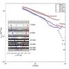 |
Fig. 18 Variation of the core shift with frequency as obtained from our reference model. The inset panel shows a contour plot of the synthetic radio maps over-plotted with corresponding core position for different observing frequencies. In the inset panel the range from −1.5 × 1018 cm < x < 0 cm indicates the jet (pointing towards the observer) and the range from 0 mas < x < 1.5 × 1018 cm corresponds to the counter-jet. |
4. Summary and outlook
We investigated the connection between jets in an ambient medium of decreasing pressure surrounded by a stationary torus. We then simulated jets using the state-of-the art SRHD code Ratpenat (Perucho et al. 2010) and included a stationary torus. The properties of the torus were motivated by both observations and theoretical modelling. In the post-processing we used a newly developed emission code and computed the thermal and non-thermal emission. To investigate the effect of the scaling parameters on the observed emission (single-dish spectra and multi-frequency radio maps) we performed a detailed parameter study and produced observable signatures, which can be used to distinguish between different jet, ambient medium, and torus configurations based on single-dish and VLBI observations. We applied a core-shift analysis to the synthetic radio maps produced and demonstrated how one can distinguish between OP jets and PM jets depending on the slope of the core shift. Our simulations and the extensive analysis of the parameter space study have shown that the observed emission is the result of a delicate interplay between hydrodynamical effects and emission and absorption processes.
A particularly robust result of this analysis is that the observed spectra of PM jets exhibit higher flux densities than the spectra of OP jets. This is because the initial pressure mismatch at the jet nozzle causes the OP jets to expand faster and convert internal energy into kinetic energy more efficiently than PM jets. At large viewing angles, the emission is strongly de-boosted for faster jets and, as a result, less emission is received by the observer. Also, while the spectra alone make it difficult to distinguish these two types of jets, high-frequency radio maps show a clear difference in both the morphology of the jet and evolution of the flux density along the jet. More specifically, apart from the core region, OP jets exhibit local maxima in the flux density at the position of the recollimation shocks (see Fig. 14). On the other hand, in PM jets the flux density decreases continuously along the jet axis outside the core region Gómez et al. (1997), Mimica et al. (2009), Fromm et al. (2016).
Another important result of our analysis is that the inclusion of a stationary torus in the synthetic emission consistently leads to a strong absorption in the single-dish spectrum. This behaviour is mostly due to the enhanced rest-mass density between the jet and observer, which in turn increases the opacity along the line of sight. Additionally, depending on properties of the torus, the spectrum flattens within a certain frequency range. Overall, the geometry of the torus has the greatest influence on the observed spectrum. In particular, increasing the geometrical size of the torus leads to a longer path for the rays generated in the jets, which then pass through a high rest-mass density field, thereby increasing the opacity along the line of sight. Indeed, if the torus is large enough and its rest-mass density sufficiently high, it can block a considerable fraction of the jet, which then becomes invisible to an observer. This effect is reflected in the flattening of the spectrum, in the appearance of an emission gap between the jet and counter-jet in the synthetic radio maps, and in optically thick spectral-index maps. Since the thermal absorption coefficient scales as ν-3, the aforementioned effects are frequency dependent, i.e. the spectra including a torus should converge to that without a torus for ν> 1011 Hz, with the emission gap between the jet and counter-jet vanishing with increasing frequency. Observationally, therefore, the spectral break could be used to constrain the rest-mass density within the torus. Given a dense frequency sampling, such as that used in the FGamma programme (Fuhrmann et al. 2016), the rest-mass density of the torus, together with additional emission parameters, can in principle be fitted.
This behaviour and in particular the frequency dependence of the synthetic radio maps can be used to distinguish between OP and PM jets. In particular, since the gap is frequency dependent, the observed onset of the jet and counter-jet varies with frequency. At low frequencies the torus should block the observer’s view and the onset of the jets are separated by an emission gap; at such frequencies, OP and PM jets are indistinguishable. However, at higher observing frequencies the gap between the jets decreases, exposing the differences in the two types of jets. Since one of the key features of OP jets are recollimation shocks, which lead to local maxima in the pressure and rest-mass density along the jet, their presence becomes visible as a local enhancement of the emission. At a certain frequency, the onset of the jet coincides with the position of a recollimation shock, which itself is frequency independent and does not change until the upstream region becomes optically thinner and brighter than the recollimation shock. This effect leads to the formation of plateaus in the core-shift plot. Because the behaviour described above is absent in the case of PM jets, for which no strong recollimation shocks are formed and no plateaus in the core shift occur, observations should be able to provide information to discriminate between these two basic classes of jets. More specifically, using multi-frequency VLBI observations, the size of the torus can be estimated by the dimensions of the optically thick region in the spectral index maps. The frequency-dependent size of the emission gap can be used to obtain estimates of the rest-mass density of the torus and analysis of the core shift would enable one to differentiate between OP and PM jets.
The simulations performed in this work were able reproduce some of the observed properties of jets from radio galaxies. However, a more detailed treatment of the torus, in particular relaxing the assumption of homogeneity, i.e. using a clumpy torus could lead to more complex single-dish spectra and radio maps. Including an independent treatment of the magnetic field, i.e. switching from SRHD to SRMHD simulations would enable us to test the influence of higher magnetisation on the non-thermal emission. Owing to the 2D axisymmetric SRHD set-up, the jets are very stable against hydrodynamical instabilities. Therefore, future studies should include 3D SRMHD in order to test the stability of the jets against hydrodynamical and magneto-hydrodynamical instabilities.
In a follow-up paper we will address some of the above-mentioned simplifications and apply the techniques presented here to actual observational data and include the propagation of shock waves using the so-called “slow-light” approach, which will enable us to investigate the temporal variations in the single-dish spectra and multi-frequency radio maps.
See Appendix for a resolution study.
We used unprimed variables for the co-moving frame and primed variables for the observer frame.
Acknowledgments
Support comes from the ERC Synergy Grant “BlackHoleCam – Imaging the Event Horizon of Black Holes” (Grant 610058). M.P. acknowledges support by the Spanish “Ministerio de Economía y Competitividad” grants AYA2013-48226-C3-2-P and AYA2015-66899-P. Z.Y. acknowledges support from an Alexander von Humboldt Fellowship. E.R. acknowledges support from the grants AYA-2012-38491-C02-01, AYA2015-63939-C2-2-P, and PROMETEOII/2014/057. C.M.F. wants to thank Walter Alef and Helge Rottmann for support during the computation on the MPIfR cluster and Mariafelicia De Laurentis and Hector Olivares for fruitful discussion and helpful comments to the manuscript.
References
- Antonucci, R. 1993, ARA&A, 31, 473 [Google Scholar]
- Crusius, A., & Schlickeiser, R. 1986, A&A, 164, L16 [NASA ADS] [Google Scholar]
- Daly, R. A., & Marscher, A. P. 1988, ApJ, 334, 539 [NASA ADS] [CrossRef] [Google Scholar]
- Falle, S. A. E. G. 1991, MNRAS, 250, 581 [NASA ADS] [CrossRef] [Google Scholar]
- Fanaroff, B. L., & Riley, J. M. 1974, MNRAS, 167, 31 [NASA ADS] [CrossRef] [Google Scholar]
- Fromm, C. M., Ros, E., Perucho, M., et al. 2013, A&A, 557, A105 [NASA ADS] [CrossRef] [EDP Sciences] [Google Scholar]
- Fromm, C. M., Perucho, M., Mimica, P., & Ros, E. 2016, A&A, 588, A101 [NASA ADS] [CrossRef] [EDP Sciences] [Google Scholar]
- Fuhrmann, L., Angelakis, E., Zensus, J. A., et al. 2016, A&A, 596, A45 [NASA ADS] [CrossRef] [EDP Sciences] [Google Scholar]
- Gómez, J. L., Marti, J. M., Marscher, A. P., Ibanez, J. M., & Alberdi, A. 1997, ApJ, 482, L33 [NASA ADS] [CrossRef] [Google Scholar]
- Hardcastle, M. J., & Krause, M. G. H. 2013, MNRAS, 430, 174 [NASA ADS] [CrossRef] [Google Scholar]
- Hoenig, S. F. 2013, ArXiv e-prints [arXiv:1301.1349] [Google Scholar]
- Joshi, M., & Böttcher, M. 2011, ApJ, 727, 21 [NASA ADS] [CrossRef] [Google Scholar]
- Kharb, P., O’Dea, C. P., Baum, S. A., et al. 2008, ApJS, 174, 74 [NASA ADS] [CrossRef] [Google Scholar]
- Komissarov, S. S., & Falle, S. A. E. G. 1997, MNRAS, 288, 833 [NASA ADS] [CrossRef] [Google Scholar]
- Laing, R. A., & Bridle, A. H. 2002, MNRAS, 336, 328 [NASA ADS] [CrossRef] [Google Scholar]
- Lister, M. L., Aller, H. D., Aller, M. F., et al. 2009, AJ, 137, 3718 [NASA ADS] [CrossRef] [Google Scholar]
- Lobanov, A. P. 1998, A&A, 330, 79 [NASA ADS] [Google Scholar]
- Mimica, P., Aloy, M. A., Agudo, I., et al. 2009, ApJ, 696, 1142 [NASA ADS] [CrossRef] [Google Scholar]
- Mizuno, Y., Gómez, J. L., Nishikawa, K.-I., et al. 2015, ApJ, 809, 38 [NASA ADS] [CrossRef] [Google Scholar]
- Pen, U.-L. 1999, ApJS, 120, 49 [NASA ADS] [CrossRef] [Google Scholar]
- Perucho, M., & Martí, J. M. 2007, MNRAS, 382, 526 [NASA ADS] [CrossRef] [Google Scholar]
- Perucho, M., Martí, J. M., Cela, J. M., et al. 2010, A&A, 519, A41 [NASA ADS] [CrossRef] [EDP Sciences] [Google Scholar]
- Porth, O., & Komissarov, S. S. 2015, MNRAS, 452, 1089 [NASA ADS] [CrossRef] [Google Scholar]
- Rezzolla, L., & Zanotti, O. 2013, Relativistic Hydrodynamics (Oxford University Press) [Google Scholar]
- Rybicki, G. B., & Lightman, A. P. 1986, Rad. Process. Astrophys., 400 [Google Scholar]
- Schartmann, M., Meisenheimer, K., Camenzind, M., Wolf, S., & Henning, T. 2005, A&A, 437, 861 [NASA ADS] [CrossRef] [EDP Sciences] [Google Scholar]
- Stalevski, M., Fritz, J., Baes, M., Nakos, T., & Popović, L. Č. 2012, MNRAS, 420, 2756 [NASA ADS] [CrossRef] [Google Scholar]
- Stalevski, M., Ricci, C., Ueda, Y., et al. 2016, MNRAS, 458, 2288 [NASA ADS] [CrossRef] [Google Scholar]
- Sutherland, R. S., & Bicknell, G. V. 2007, ApJS, 173, 37 [NASA ADS] [CrossRef] [Google Scholar]
- Urry, C. M., & Padovani, P. 1995, PASP, 107, 803 [NASA ADS] [CrossRef] [Google Scholar]
- van Hoof, P. A. M., Williams, R. J. R., Volk, K., et al. 2014, MNRAS, 444, 420 [NASA ADS] [CrossRef] [Google Scholar]
Appendix A:
We performed a convergence test for our emission calculations and the results are presented in Fig. A.1. For the test we used the reference model (see Table 2) and increased the number of cells used in the computation in 1003 steps. In Fig. A.1 we show the single-dish spectrum between 1 GHz and 1 THz for different resolutions and the inset panel shows the variation of the total flux density with respect to the number of simulation grid cells. The calculated flux density converges to a common value and no significant differences was obtained above 4003 cells. At the lowest resolution (1003) the high-frequency flux density is significantly different compared to the high resolution runs. This difference occurred since the high-frequency emission was created close to the jet nozzle and therefore emanates from a region of small transversal jet size. If the resolution was not sufficiently high to resolve these regions, the triangulation and interpolation of these cells onto the 3D grid failed (overestimating the contribution from the ambient medium) and led to unphysically low flux densities.
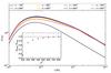 |
Fig. A.1 Convergence test for the emission calculations. Single-dish spectrum for seven different resolutions. |
Similar to the test on emission calculations we conducted a convergence study of the SRHD simulations. For this study we employed the procedure described in Sect. 2, increasing the numerical resolution by a factor 2, resulting in 4, 8, and 16 cells per jet radii. We simulated both, a PM and OP jet using the initial conditions presented in Table 2. A steady state was obtained and after roughly after 5 to 6 longitudinal grid crossing times, we computed the emission with a fixed detector frame resolution of 3003 cells. In Fig. A.2 we present the result of the convergence study on the SRHD simulations. The solid lines correspond to the PM jet (dk = 1) and the dashed lines to the OP jet (dk = 2.5). The result of this study shows that our initial resolution of 4 cells per jet radii can reproduce 95% of the total flux density obtained from the simulation with the highest resolution in the case of PM jets and 90% in the case of OP jets. Since we are mainly interested in emission from the large-scale structure, 4 cells per jet radii represents a sufficient resolution for our study. However, a higher resolution would be needed to sufficiently resolve the structure induced by travelling shocks and study the time variability of non-thermal emission from the jets.
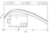 |
Fig. A.2 Convergence test for the SRHD calculations. Single-dish spectrum for three different resolutions for both PM jet (solid lines) and OP jet (dashed lines). |
All Tables
All Figures
|
Fig. 1 Distribution of ambient pressure and ambient rest-mass density in code units for the gradients in the ambient medium. |
| In the text | |
|
Fig. 2 Geometry of the assumed torus model (adapted from Stalevski et al. 2012). |
| In the text | |
|
Fig. 3 Left panel: distribution of temperature in the meridional plane. Right panel: corresponding rest-mass density distribution. The Θ-dependence in the distribution of the temperature and the rest-mass density is clearly visible. |
| In the text | |
|
Fig. 4 Example of the 3D geometry of the jet-torus model. |
| In the text | |
|
Fig. 5 Stationary results for the jet simulations. The panels show the 2D distribution of the rest-mass density for different ambient medium configurations as indicated by the exponent m. In each panel the left side (−30 <r/Rj< 0) corresponds to the OP jet and the right side (0 <y/Rj< 30) to the PM jet. The top row spans the entire simulation grid whereas the bottom row shows a magnified view of the nozzle region (−7 <z/Rj< 7). The white lines in the bottom row show stream lines visualising the direction of the flow and the bold dashed lines correspond to the inward travelling and reflected shock wave. |
| In the text | |
 |
Fig. 6 Same as Fig. 5 for the pressure. |
| In the text | |
|
Fig. 7 Variation of the jet parameters along the jet axis. The left column corresponds to OP jets and the right column to PM jets. From top to bottom: the jet radius, axial pressure, and axial velocity in the z-direction are shown (see text for details). |
| In the text | |
|
Fig. 8 Single-dish spectra for a simulation including a torus (black) and without a torus (red). |
| In the text | |
|
Fig. 9 Single-dish spectra for the different jet and ambient medium models. |
| In the text | |
|
Fig. 10 Influence of the scaling parameters Rj, ϑ, and Lkin on the shape of the observed single-dish spectrum. |
| In the text | |
|
Fig. 11 Influence of the emission parameters ρa,ϵe,ϵb,ζe,ϵγ, and s on the shape of the observed single-dish spectrum. |
| In the text | |
|
Fig. 12 Influence of the torus parameter on the observed single-dish spectrum. Top row from left to right: the torus outer radius, torus thickness, and torus rest-mass density are shown. Bottom row from left to right: the torus temperature, distribution of the torus rest-mass density, and distribution of the torus temperature are shown. |
| In the text | |
|
Fig. 13 Convolved radio maps at 15 GHz. In each panel the range from −3 × 1018 cm <x< 0 cm indicates the jet (pointing towards the observer) and the range from 0 mas <x< 3 × 1018 cm corresponds to the counter-jet. The panels correspond to different gradients used in the ambient medium indicated by n and m. In each panel the the top half corresponds to an OP jet and the bottom half to a PM jet. The convolving beam is plotted in bottom left corner of each panel. |
| In the text | |
|
Fig. 14 Same as Fig. 13 at a frequency of 86 GHz. In each panel the range from −1.5 × 1018 cm <x< 0 cm indicates the jet (pointing towards the observer) and the range from 0 mas <x< 1.5 × 1018 cm corresponds to the counter-jet. The panels correspond to different gradients used in the ambient medium indicated by n and m. In each panel the top half corresponds to an OP jet and the bottom half to a PM jet. The convolving beam is plotted in the bottom left corner of each panel. |
| In the text | |
|
Fig. 15 Influence of the viewing angle (left column), the thermal to non-thermal energy ratio (middle column) and the torus rest-mass density (right column) on the 15 GHz radio maps. In each panel the range from −3 × 1018 cm <x< 0 cm indicates the jet (pointing towards the observer) and the range from 0 mas <x< 3 × 1018 cm corresponds to the counter-jet. The convolving beam is plotted in the bottom left corner of each panel. |
| In the text | |
|
Fig. 16 Spectral index maps computed between 22 GHz and 43 GHz for various torus densities. In each panel the range from −3 × 1018 cm < x < 0 cm indicates the jet (pointing towards the observer) and the range from 0 mas < x < 3 × 1018 cm corresponds to the counter-jet. The convolving beam is plotted in the bottom left corner of each panel. |
| In the text | |
|
Fig. 17 Synthetic multi-frequency radio maps from 8 GHz to 86 GHz. In each panel the range from −3 × 1018 cm < x < 0 cm indicates the jet (pointing towards the observer) and the range from 0 mas < x < 3 × 1018 cm corresponds to the counter-jet. The convolving beam is plotted in the bottom left corner of each panel. |
| In the text | |
|
Fig. 18 Variation of the core shift with frequency as obtained from our reference model. The inset panel shows a contour plot of the synthetic radio maps over-plotted with corresponding core position for different observing frequencies. In the inset panel the range from −1.5 × 1018 cm < x < 0 cm indicates the jet (pointing towards the observer) and the range from 0 mas < x < 1.5 × 1018 cm corresponds to the counter-jet. |
| In the text | |
|
Fig. A.1 Convergence test for the emission calculations. Single-dish spectrum for seven different resolutions. |
| In the text | |
|
Fig. A.2 Convergence test for the SRHD calculations. Single-dish spectrum for three different resolutions for both PM jet (solid lines) and OP jet (dashed lines). |
| In the text | |
Current usage metrics show cumulative count of Article Views (full-text article views including HTML views, PDF and ePub downloads, according to the available data) and Abstracts Views on Vision4Press platform.
Data correspond to usage on the plateform after 2015. The current usage metrics is available 48-96 hours after online publication and is updated daily on week days.
Initial download of the metrics may take a while.