| Issue |
A&A
Volume 693, January 2025
|
|
|---|---|---|
| Article Number | A154 | |
| Number of page(s) | 10 | |
| Section | Astrophysical processes | |
| DOI | https://doi.org/10.1051/0004-6361/202451573 | |
| Published online | 15 January 2025 | |
Numerical investigation of instabilities in over-pressured magnetized relativistic jets
1
Tsung-Dao Lee Institute, Shanghai Jiao-Tong University, 1 Lisuo Road, Shanghai 201210, People’s Republic of China
2
School of Physics & Astronomy, Shanghai Jiao-Tong University, 800 Dongchuan Road, Shanghai 200240, People’s Republic of China
3
Institut für Theoretische Physik, Goethe Universität, Max-von-Laue-Str. 1, D-60438 Frankfurt, Germany
4
Institut für Theoretische Physik und Astrophysik, Universität Würzburg, Emil-Fischer-Str. 31, D-97074 Würzburg, Germany
5
Max-Planck-Institut für Radioastronomie, Auf dem Hügel 69, D-53121 Bonn, Germany
⋆ Corresponding author; mizuno@sjtu.edu.cn
Received:
19
July
2024
Accepted:
26
November
2024
Context. Relativistic jets from active galactic nuclei are observed to be collimated on the parsec scale. When the pressure between the jet and the ambient medium is mismatched, recollimation shocks and rarefaction shocks are formed. Previous numerical simulations have shown that instabilities can destroy the recollimation structure of jets.
Aims. In this study, we aim to study the instabilities of nonequilibrium over-pressured relativistic jets with helical magnetic fields. Especially, we investigate how the magnetic pitch affects the development of instabilities.
Methods. We performed 3D relativistic magnetohydrodynamic simulations for different magnetic pitches, as well as a 2D simulation and a relativistic hydrodynamic simulation which served as comparison groups.
Results. In our simulations, Rayleigh-Taylor instability (RTI) is triggered at the interface between the jet and ambient medium in the recollimation structure of the jet. We find that when the magnetic pitch decreases, the growth of RTI becomes weak but, interestingly, another instability – the current-driven (CD) kink instability – is excited. The excitement of CD kink instability after passing the recollimation shocks can match the explanation of the quasi-periodic oscillations observed in BL Lac qualitatively.
Key words: accretion / accretion disks / magnetohydrodynamics (MHD) / plasmas / galaxies: jets
© The Authors 2025
 Open Access article, published by EDP Sciences, under the terms of the Creative Commons Attribution License (https://creativecommons.org/licenses/by/4.0), which permits unrestricted use, distribution, and reproduction in any medium, provided the original work is properly cited.
This article is published in open access under the Subscribe to Open model. Subscribe to A&A to support open access publication.
1. Introduction
Relativistic jets, one of the most remarkable features of supermassive black holes (SMBHs), have drawn the widespread attention of scientists since it was first recorded in 1918 (Curtis 1918). Relativistic jets have enormous power and move at relativistic speeds (i.e., high Lorentz factors), causing the observations of superluminal motion. Although a hundred years passed since the first discovery, the mechanism of jet launching is still under debate. There are two major mechanisms for jet launching: one is the direct energy extraction of a rotating black hole by the Blandford-Znajek mechanism (Blandford & Znajek 1977) and the other is the acceleration by the magneto-centrifugal force from the accretion disk that is known as the Blandford-Payne mechanism (Blandford & Payne 1982).
Through the observations from the radio to the X-ray regime, we know relativistic jets in active galactic nuclei (AGNs) are highly collimated on a scale from subparsecs to megaparsecs (Pushkarev et al. 2009). When a jet propagates through an ambient medium, a pressure mismatch between the jet and the ambient medium arises as a result of changing the pressure of the ambient medium. The pressure mismatch drives a radial oscillating motion of the jet that leads to multiple recollimation regions inside the jet (e.g., Gómez et al. 1997; Komissarov & Falle 1997; Agudo et al. 2001; Porth & Komissarov 2015; Mizuno et al. 2015; Fromm et al. 2016). Such recollimation shocks would be connected to the quasi-stationary features seen in jets of AGNs (e.g., Jorstad et al. 2005; Lister et al. 2013; Cohen et al. 2014; Gómez et al. 2016). The case of M87 is very interesting because the stationary feature HST-1 knot is thought to be related to a recollimation shock and we see the emergence of new superluminal components from HST-1 (Giroletti et al. 2012). In addition, very high-energy emission is associated with the variability of the HST-1 region (Cheung et al. 2007).
During the propagation of the jets to large scales, several instabilities can grow which could lead to a loss of collimation and even destroy the jet. The observed morphological differences of relativistic jets could also be linked to a physical reason for the Fanaroff-Riley dichotomy (Fanaroff & Riley 1974). For example, a Poynting-flux-dominated jet with a large-scale helical magnetic field is unstable under the current-driven instability (CDI), in particular, to the kink mode (e.g., Moll et al. 2008; Mizuno et al. 2009, 2014). In such a situation, the shape of the jet changes to a helically twisted structure. Another possible instability is Kelvin-Helmholtz instability (KHI). In the presence of velocity shear, it leads to small amplitude wave-like disturbances on the interface. Centrifugal instability (CFI) can be excited within the rotational jet (Gourgouliatos & Komissarov 2018) that forms mushroom shapes on the interface at a regular angle interval in 2D sections perpendicular to the jet propagation direction. However, a weak toroidal magnetic field stabilizes against this instability (Komissarov et al. 2019; Matsumoto et al. 2021). The Rayleigh-Taylor instability (RTI) is also possible to grow at the boundary of the jet and external medium which is characterized by a finger-like structure (Keppens & Meliani 2012). Generally, it is difficult to derive the stability condition for each instability in the jet analytically because the jets are subject to a complicated nonlinear interplay between jet rotation, magnetic fields, relativistic effects, the structure between the jet and external medium, etc.
Adopted by a large number of previous works, relativistic magnetohydrodynamic (RMHD) simulations are proven to be an effective method for studying the propagation and stability of the jet. Mizuno et al. (2015) have simulated over-pressured jets with and without magnetic fields in 2D. All of the jets showed the development of recollimation shock structures and no instability was triggered. Matsumoto & Masada (2013) have performed 2D relativistic hydrodynamic (RHD) simulations of a co-moving over-pressured jet on the plane perpendicular to the jet. They found when the effective inertia γ2ρh of the jet is greater than that of the outer external medium, the boundary between the jet and external medium is unstable against RTI, where γ is the Lorentz factor, ρ is density, and h is the specific enthalpy. The effects of the jet rotation and toroidal magnetic field for the RTI in two-component jets have been investigated by Millas et al. (2017) and they show that the magnetic field provides stability against RTI. Abolmasov & Bromberg (2023) point out that three vectors in the RTI cannot be coplanar: the jet propagation direction, the effective gravity direction, and the unstable mode’s wave vector direction. Thus, 3D, non-axisymmetric simulations are essential for the study of RTI. Gourgouliatos & Komissarov (2018) simulated 3D RHD jets and show that the instabilities in recollimation shocks are rather related to the centrifugal instability (CFI) than to the RTI. The studies were extended to 3D MHD simulations by Matsumoto et al. (2021). Recently, Costa et al. (2024) tried to use 3D HD simulations to explain morphologies of the FR0 type of jets (Ghisellini 2011) observed by Very Long Baseline Interferometry (VLBI). In this paper, we extend our previous 2D RMHD simulations of over-pressured jets with the helical magnetic field by Mizuno et al. (2015) to 3D non-axisymmetric simulations. As we discussed, 3D, non-axisymmetric simulations are essential for the study of instabilities in the jet. We investigate how the helical magnetic field affects the stability of overpressured jets.
The structure of this paper is as follows. In Section 2, we present our method and the setup of the 3D RMHD simulations. In Sections 3.1 and 3.2, we first show the 2D RMHD and 3D RHD simulations of an over-pressured jet. In Section 3.3, we compare the results of the 3D RMHD simulations with helical magnetic field and discuss the effect of magnetic pitches. We analyze the recollimation shock structure and the possibility of the excitement of kink instability in Section 4, and also summarize and discuss our findings there.
2. Numerical setup
We performed 3D RMHD simulations of over-pressured jets using the public RMHD code PLUTO (Mignone et al. 2007) adopting cartesian coordinates. We solved the following form of the RMHD equations:
where b0 = γv ⋅ B, b = B/γ + γ(v ⋅ B)v, ωt = ρh + B2/γ + (v ⋅ B)2, and pt = pgas + [B2/γ2 + (v ⋅ B)2]/2. We set c = 1 and the units of velocity, density, pressure, and magnetic field strength are c, ρ0, ρ0c2, and  , respectively. The specific enthalpy is defined as h = 1 + Γpgas/(Γ − 1)ρ and magnetization is σ = |b|2/ρ. We used the ideal equation of state with the adiabatic index Γ = 4/3.
Table 1 shows the basic numerical setup and numerical methods that we used in our simulations. As following previous work by Mizuno et al. (2015), we consider the cylindrical over-pressured jet to be filled in the simulation domain. The jet radius is Rj = 1. It has an axial velocity with a Lorenz factor γj = 3 which corresponds to vj = 0.9428c. The jet is lighter (ρj = 0.01) and over-pressured (pj = 1.5pa) than the ambient medium initially. The ambient medium is stationary (va = 0) with a constant density (ρa = 1) and constant gas pressure (pa = 0.018). A preexisting cylindrical jet has a helical magnetic field. The poloidal and toroidal components of the magnetic field are given by
Setup of our 3D RMHD simulations.
where we used B0 = 0.2 in fiducial models. We note that a and k are parameters related to determining the magnetic pitch profile:
In our fiducial model (MHD1), we used a = 0.5 and  which leads to a magnetic pitch of P = 0.22 and an average magnetization ⟨σ⟩ = 1.33. To explore the effect of magnetic pitch, we also simulated the cases with different magnetic pitches such as k = 1 (MHD2) and
  (MHD3), which correspond to a higher pitch (P = 0.5) and a lower pitch (P = 0.16) than our fiducial model, respectively. We should note that in our definition of the magnetic pitch, the higher (lower) pitch case has a more poloidal (toroidal) component the magnetic field dominates. The case MHD2w uses a weaker magnetic field (B0 = 0.1) than the model MHD1 to discuss the effect of the magnetic field. Table 2 lists the setups of various cases. The effective inertia is nearly invariant among different cases (see Sect. 4 for details). Figure 1 shows the initial radial distribution of the toroidal magnetic field and magnetization in different cases. We set the jet radius as Rj = 1. All quantities are sharply changed at the jet boundary. As you see from the figure, in most simulation models, the jets are highly magnetized (σ > 1).
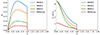 |
Fig. 1. Initial distributions of toroidal fields (the left panel) and magnetizations (the right panel) for various cases. |
Basic properties of the different cases, where ⟨σ⟩ is the averaged magnetization.
The computational domain is (x, y, z) = (±5 Rj, ±5 Rj, 60 Rj) with a uniform grid of (Nx, Ny, Nz) = (500, 500, 600). This corresponds to 50 cells per jet radii in the transversal direction and 10 cells per jet radii in the vertical direction. We imposed outflow boundary conditions on all surfaces except for z = zmin. At z = 0, we used fixed boundary conditions that continuously injected the over-pressured jet into the computational domain. All simulations were performed up to ts = 400, where the simulation time unit is ts = Rj/c.
3. Results
3.1. 2D helically magnetized jet
First, we present the 2D RMHD simulations of over-pressured jets with a helical magnetic field. For the 2D simulation (MHD1-2D), we used a cylindrical coordinate (R, z), and the axisymmetric boundary was employed at R = 0. The simulation domain is [R, z]=[5 Rj, 60 Rj] with a grid number of (NR, Nz) = (250, 600).
Figure 2 shows 2D distributions of the rest-mass density, effective inertia (I = γ2ρh + Bz2 + Bϕ2), and magnetic pitch for the 2D RMHD case at ts = 400. As pointed out by Matsumoto & Masada (2013), effective inertia is a key quantity to understand the stability of recollimation shock. Here, we present the effective inertia in the radial direction. The effective inertia is useful to investigate the recollimation shock structure analytically. A detailed discussion is provided in Appendix A.
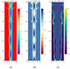 |
Fig. 2. Distribution of the logarithmic density (left), effective inertia, I = γ2ρh + Bz2 + Bϕ2 (middle), and magnetic pitch (right) for the 2D RMHD model MHD1-2D at ts = 400. |
From the beginning of the simulation, due to the jet being over-pressured than the external medium initially, shocks and rarefaction waves are created at the boundary of the jet and the external medium. These propagate inside and outside the jet to make a recollimation shock structure as seen in Mizuno et al. (2015). The jet appears to be a stable recollimation shock structure as shown in Fig. 2. The separation of recollimation shocks is mostly constant due to the constant external medium. The plot of the effective inertia (the middle panel) shows a low inertia interface between the jet and the ambient environment. This is because the gas at the interface is less dense than the environment and it has a lower Lorentz factor than the inner jet. Meanwhile, the right panel of Fig. 2 illustrates that the magnetic pitch also forms a boundary at the interface and the outer part shows a hierarchical structure. Some peculiar structures are visible outside the jet at z > 40, which are components ejected by the jet during the establishment of recollimation structures. Thus, these are kinds of numerical artifacts. Similar to Mizuno et al. (2015), in 2D simulations, we did not see any excitement of the instabilities in jets. From the analytical approach, we could mostly reproduce the radial motion of the recollimation shock structure (see Appendix A).
3.2. 3D hydrodynamic jet
We performed 3D RHD simulations of an over-pressure jet that is marked as the case HD. The results are shown in Fig. 3. From the density distribution, we clearly see the development of instability at the jet boundary. After creating the first recollimation shock structure at z = 10 Rj, the jet begins to transform into turbulence by growing the instability before forming a complete recollimation structure. Figure 4 shows the distribution on the xy plane of density and the Lorentz factor at two different axial positions that indicate the development of RTI at different distances from the inlet. At z = 15 Rj (top panels), we see finger-like structures at the boundary between the jet and ambient medium, which are typical characteristics of RTI. In the further distance from the jet inlet (z = 30 Rj), RTI is well developed and tends to have a nonlinear evolution, which leads to the turbulent structure with the mixing layer of the jet and ambient medium. From the Lorentz factor plots, we see the jet is accelerated during this development.
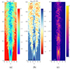 |
Fig. 3. 2D axial distribution of logarithmic density (a), effective inertia, I = γ2ρh (b), and the Lorentz factor (c) for the 3D RHD case HD at ts = 400. |
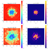 |
Fig. 4. Distribution on the xy plane of density (left) and the Lorentz factor (right) at z = 15 Rj (top) and z = 30 Rj (bottom) for the HD case at ts = 400. |
In our 3D RHD simulation, the initial effective inertia of jet Ij = γ2ρh = 1.062 is slightly smaller than the ambient environment (Ia = 1.072). Our 3D RHD simulation satisfies the stability condition by Matsumoto & Masada (2013). However, later Matsumoto et al. (2017) provided an updated analytical stability criterion for RTI in the following form:
![$$ \begin{aligned} \left[\gamma ^2\rho \left(1+\frac{\Gamma ^2}{\Gamma -1}\frac{p_{\rm gas}}{\rho }\right)\right]_{j} < \left[\gamma ^2\rho \left(1+\frac{\Gamma ^2}{\Gamma -1}\frac{p_{\rm gas}}{\rho }\right)\right]_{a}, \end{aligned} $$](/articles/aa/full_html/2025/01/aa51573-24/aa51573-24-eq13.gif)
which is slightly different from the definition of effective inertia, I = γ2ρh. Based on this updated analytical stability criteria, our simulation condition does not satisfy this stability condition, which indicates RTI can grow in our 3D RHD simulation. The prediction of the criterion is consistent with the simulation.
3.3. 3D helically magnetized jet
In the previous subsection, we have shown that a recollimation shock structure is stable in 2D axisymmetric RMHD simulations of over-pressured jets with a helical magnetic field. However, in 3D RHD simulations, we see the development of RTI. We subsequently performed 3D RMHD simulations of over-pressured jets with a helical magnetic field.
The fiducial model takes the same numerical setup as the 2D RMHD simulation shown in Section 3.1. In Fig. 5, we show the distributions of density, effective inertia, and magnetization σ of the MHD1 at ts = 365, where the form of magnetization σ = Bϕ2/γ2ρ, which was used in Millas et al. (2017). We should note that, unfortunately, the simulation was stopped at t = 365 due to numerical reasons. However, the development of RTI is saturated around ts = 250 (see Fig. 7). Thus we think the distribution at ts = 365 is still comparable with other cases shown at ts = 400.
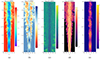 |
Fig. 5. 2D axial distribution of logarithmic density (a), effective inertia (b), magnetic pitch (c), magnetization (d), and the Lorentz factor (e) for the 3D RMHD case MHD1 at ts = 365. |
In the comparison with the 2D RMHD case, we clearly see the development of the RTI that is triggered in the 3D simulation. In the region far from the jet inlet, RTI is fully developed, and the turbulent structure is excited. Moreover, from the plot of effective inertia, we can observe that the low inertia interface still exists in the turbulent region and it also develops finger-like structures, separating inner and outer turbulence. Unlike the 2D case, the magnetic pitch in the 3D case shows a complex structure. As Matsumoto et al. (2017) indicated, the difference in effective inertia between the jet and the ambient medium does not give a criterion for the growth of the RTI. However, it is still useful to trace the recollimation shock structure (see Appendix A).
The panel c of Fig. 5 implies the RTI is triggered even when the region with high magnetization σ > 10. It seems a contradiction to the statement that higher magnetization (σ > 0.01) stabilizes the jet suggested by Millas et al. (2017). However, in their simulations, they used a pressure continuity condition at the boundary while we considered over-pressure jets. This may indicate that it would be difficult to derive a quantitative stability criterion due to the complex properties of the jet.
Similar to Fig. 4, Fig. 6 shows the distribution on the xy plane of density and the Lorentz factor at two different axial positions that indicate the development of RTI at different distances from the jet inlet. Obviously, the existence of the toroidal magnetic field slows down the development of RTI.
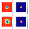 |
Fig. 6. Distribution on the xy plane of density and the Lorentz factor at z = 15 Rj (top) and z = 30 Rj (bottom) for the MHD1 case at ts = 365. |
To quantitatively analyze the strength of RTI among different cases, we plotted the time evolution of average radial velocity |vr|/c at z = 60 Rj for the HD, MHD-2D, and MHD1 cases, respectively, in Fig. 7. The recollimation shock starts to develop on the top of the simulation box at ts = 64 and a jet reaches a fully developed state at ts = 100. After that, stable recollimation shock structures are formed in the 2D RMHD case (MHD-2D) that indicates the ⟨|vr|/c⟩∼0. However, for the 3D RHD case (HD), the RTI starts to grow after the recollimation shock develops. Thus, the averaged radial velocity grows continuously in a later simulation time due to the development of a turbulent structure. For the 3D RMHD case (MHD1), the magnetic field, in particular the toroidal field, eliminates the development of RTI. It is indicated that the strength of average radial velocity becomes smaller than that in the HD case. We note that an axial variation by the development of instability depends a little on the spatial resolutions. However, the results do not change it.
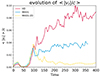 |
Fig. 7. Time evolution of averaged radial velocity |vr|/c at z = 60 Rj with the cases of 3D RHD (HD, red), 2D RMHD (MHD1-2D, dashed yellow), and 3D RMHD (MHD1, blue). |
3.4. Effects of magnetic strength and pitches
We continued our investigation by comparing the simulation results with different magnetic pitch cases, lower magnetic pitch (MHD2) with P = 0.16, and higher magnetic pitch (MHD3) with P = 0.5. Figure 8 shows the density distributions at ts = 400.
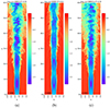 |
Fig. 8. 2D axial distribution of the logarithmic density for the cases of different magnetic pitches and magnetic strength at ts = 400. (a) Higher magnetic pitch case (MHD2) with k = 1 and P = 0.50, (b) lower magnetic pitch case (MHD3) with |

When the magnetic pitch becomes higher (MHD2; left panel of Fig. 8), the RTI grows faster. Thus, the jet is more disrupted in the further region from the jet inlet than in the case of MHD1. On the other hand, with the magnetic pitches decreasing (case MHD3; middle panel of Fig. 8), the RTI is mostly prohibited as is also indicated by Millas et al. (2017) and Matsumoto et al. (2021).
Figure 9 shows the time evolution of the averaged radial velocity at z = 60 Rj for three different magnetic pitch cases. From this figure, we clearly see that the lower pitch case (green line) has a larger averaged radial velocity than our fiducial model (blue line). When the magnetic pitch becomes higher (purple line), the averaged radial velocity significantly reduces. Thus, the magnetic pitch is crucial for the growth of RTI.
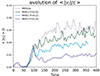 |
Fig. 9. Same as Fig. 7 but for cases with different magnetic pitches. The green line represents the higher magnetic pith case MHD2 (k = 1 and P = 0.5) and the purple line indicates the lower magnetic pitch case MHD3 case ( |

As seen in Fig. 7, the existence of a magnetic field reduces the development of RTI. When the magnetic field becomes weaker, the growth of RTI becomes stronger as is seen in the right panel of Fig. 8. From the time evolution of the averaged radial velocity (dotted line of Fig. 9), the weaker RMHD case MHD2w is properly between the MHD1 case and the HD case (see in Fig. 7). This indicates that the magnetic field strength is an important factor for the development of RTI.
When the RTI no longer fully disrupts the jet structure in higher magnetic pitch cases such as the MHD3 case (the middle panel in Fig. 8), we can see the helically twisted structure in the jets. This implies evidence of growing current-driven kink instability (e.g., Mizuno et al. 2014; Singh et al. 2016). We are going to discuss this in the following Section 3.6.
3.5. Possibility of other instabilities
In our 3D MHD simulation of an over-pressured jet, we have seen the growth of instability at the boundary between the jet and external medium that disrupts the jet structure. From the finger-like structure seen at the boundary and condition, we concluded it is due to the growth of RTI. However, other instabilities such as KHI, Richtmyer–Meshkov instability (RMI), and CFI can also contribute to the disruption of the jet except for RTI. In this subsection, we evaluate the possibility of each instability.
For our simulations, KHI is mostly ruled out because initially, we did not have such a velocity shear boundary. We note that RTI is some kind of KHI.
RMI may be excited when the reflective shock from the jet axis reaches the contact continuity at the boundary. For the MHD1 case, as is shown in the distribution of effective inertia at the xy plane of Fig. 10, reflective shock is observed around z = 12. However, there is no clear evidence of the growth of RMI as was seen in Matsumoto & Masada (2013) when the shock reached the contact discontinuity.
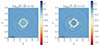 |
Fig. 10. Distributions on the xy plane of effective inertia at z = 12 Rj (the left panel) and z = 13 Rj (the right panel) for the MHD1 case at ts = 365. |
From the previous studies by Komissarov et al. (2019) and Matsumoto et al. (2021), CFI can possibly grow in relativistic magnetized jets. However, it is also known that a weak magnetic field can inhibit it. Based on the definition of magnetization σm = bϕ2/ρh, Matsumoto et al. (2021) mention that when the jet magnetization becomes larger than 0.01, the CFI is stabilized. Under this definition, we calculated the maximum magnetizations for our MHD cases. These are 0.047 (MHD1), 0.0094 (MHD2), 0.094 (MHD3), and 0.0023 (MHD2w), respectively. Most of our cases have a higher magnetization than the criteria suggested by Matsumoto et al. (2021). Thus, we do not need to consider that the developed turbulent structure of a jet is caused by the growth of CFI.
Matsumoto et al. (2021) propose a more elaborate criterion, that is,
where θ0 is the jet opening angle. To calculate the jet opening angle, we estimated the jet radii through the approach described in Appendix A, then we calculated the initial half-opening angle of the jet. In the MHD1, MHD2, MHD3, MHD2w cases, the open angle is 0.093, 0.074, 0.082, and 0.031, and the required magnetization for stabilizing the CFI is σ > 0.0049, 0.0031, 0.0038, and 0.0064, respectively. Except for the MHD2w case, the jet should be stable to CFI. From these arguments, we conclude that the developed turbulence at the interface between the jet and external medium is caused by the development of RTI.
3.6. Kink instability in the simulations
As seen in the effect of the magnetic field in over-pressured relativistic jets, the existence of a magnetic field helps stabilize the jets against RTI. In some cases, RTI has almost ceased to grow. However, in strongly magnetized relativistic jets with helical magnetic fields, CD kink instability potentially grows. Figure 11 shows a 3D volume rendering of the density with magnetic field lines for the case MHD1 at ts = 360. At z > 30 Rj, a helically twisted jet structure is observed. A similar structure is also seen in the MHD3 case (the middle panel in Fig. 8). Helical magnetic fields also follow helically twisted density structures. A similar behavior is seen in previous 3D RMHD simulations of CD kink instability in relativistic jets (e.g., Mizuno et al. 2009, 2012, 2014; Singh et al. 2016), although some of the magnetic field lines show zigzag trajectories due to the turbulence. After the passing of recollimation shock, the toroidal magnetic field becomes stronger, and the relativistic jet remains highly magnetized. It is a good condition for the growth of CD kink instability. The development of CD kink instability after the recollimation shock is seen in 3D RMHD simulations of jet propagation in the stratified external medium (Tchekhovskoy & Bromberg 2016; Barniol Duran et al. 2017).
 |
Fig. 11. 3D density isosurface at t = 360. The white (blue) surface marks the isosurface where density equals 0.01(0.005). The yellow lines are traces of the magnetic field lines. The color scales with the logarithm of the density. |
To investigate the propagation speed of the helically twisted structure, we plotted the azimuthal-averaged density profiles at R = 1 Rj in different times with ts = 397, 398, 399, and 400 in Fig. 12. From this figure, we captured four peaks between z = 47 Rj and z = 50 Rj. Thus, the propagation speed of a helically twisted structure is about 0.8c, which is mostly consistent with the propagation speed of the jet itself. Similar results are seen in Mizuno et al. (2014) and Singh et al. (2016).
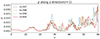 |
Fig. 12. Azimuthal average density profiles at R = 1 Rj for ts = 397 (dash-dotted blue), 398 (dashed orange), 399 (dotted green), and 400 (solid red). |
4. Summary and discussion
For this paper, we performed 3D RMHD simulations of over-pressured magnetized jets and explored the effect of the magnetic pitch and strength. We began our simulation with the 2D axisymmetric configuration and obtained a stable recollimation shock structure, retrieving the conclusion of Mizuno et al. (2015). From the simulations, we observed a low effective inertia interface between the jet and the ambient medium. By removing axisymmetric symmetry, the 3D RHD simulations of the over-pressured jets exhibited the development of RTI at the interface between the jet and ambient medium, confirming the prediction of Matsumoto et al. (2017). For 3D RMHD simulations of over-pressured jets, we observed that the recollimation shock structure transforms into a mixture of the RTI at the interface between the jet and ambient medium and the CD kink instability in the jet. As stated by Millas et al. (2017), increasing the toroidal magnetic field contribution (decreasing the magnetic pitch) stabilizes the jet against RTI. However, our simulations did not obey the suggested stability criterion that the magnetization σ > 0.01 keeps the jet stable. This implies that magnetic field configuration affects the jet stability criterion.
We derived the radial motion equation of the recollimation structure with the assumption that the radial magnetic field equals zero and the radial velocity is infinitesimal (Appendix A). The pressure gradient, magnetic pressure, and centrifugal force affect radial acceleration. We confirmed that the radial motions of jets are consistent with the prediction of this equation both in 2D and 3D cases. Although we have not obtained the analytical expression of stability criteria in this work, these three kinds of force will all play their roles in the analysis of instability. It will be included in our future study.
This study is an extension of our previous work (Mizuno et al. 2015). Thus, we assumed an external medium with a simple contact density. However, in reality, the external medium would likely be characterized by declining profiles. Several papers have discussed the effect of declining density profiles on to the jet dynamics and structures (e.g., Gómez et al. 1997, 2016; Porth & Komissarov 2015; Tchekhovskoy & Bromberg 2016; Barniol Duran et al. 2017; Fromm et al. 2019). In general, the jet has radially expanded and the distance between two recollimation shocks becomes larger with distance. We will discuss it in a separate paper.
In this work, we assumed a jet is relatively hot. However, in nature, a jet might be cold. A cold jet has a smaller effective inertia. It becomes lighter. Therefore, the deformation of the jet would be more obvious. However, if a jet is over-pressured, similarly the recollimation shock is developed and RTI disrupts the interface between a jet and an external medium. The existence of a magnetic field would stabilize the RTI as seen in this work. Thus, we expect the global picture may not change much.
In our 3D RMHD simulations with a helical magnetic field, the excitement of CD kink instability is seen after passing the recollimation shocks. Recently, Jorstad et al. (2022) suggested CD kink instability develops after passing recollimation shock to explain the quasi-periodic oscillations (QPOs) observed during the outburst in 2020 of blazar BL Lac. BL Lac has recognized the existence of multiple stationary knots (Cohen et al. 2014; Gómez et al. 2016) that would be multiple recollimation shocks. Cohen et al. (2015) suggest the existence of a helical magnetic field in relativistic jets of BL Lac. Jorstad et al. (2022) also argue that the growth of the kink with time could match the QSO properties in BL Lac. Our simulations are qualitatively consistent with their observations. We think our simulation results provide a consistent picture with the observations in BL Lac. However, in this work, our numerical setup is idealized for the investigations of instability. For future studies, we will set up the initial conditions of a simulation matched with the condition in BL Lac to obtain observables such as jet images, polarization, and light curves that are directly comparable to the observations.
Acknowledgments
This research is supported by the National Key R&D Program of China (2023YFE0101200), the National Natural Science Foundation of China (Grant No. 12273022), and the Shanghai Municipality orientation program of Basic Research for International Scientists (Grant No. 22JC1410600). CMF is supported by the DFG research grant “Jet physics on horizon scales and beyond” (Grant No. 443220636) within the DFG research unit “Relativistic Jets in Active Galaxies” (FOR 5195). The simulations were performed on the Astro cluster at Tsung-Dao Lee Institute and the Siyuan-1 cluster at the High-Performance Computing Center at Shanghai Jiao Tong University. This work has used NASA’s Astrophysics Data System (ADS).
References
- Abolmasov, P., & Bromberg, O. 2023, MNRAS, 520, 3009 [NASA ADS] [CrossRef] [Google Scholar]
- Agudo, I., Gómez, J.-L., Martí, J.-M., et al. 2001, ApJ, 549, L183 [Google Scholar]
- Barniol Duran, R., Tchekhovskoy, A., & Giannios, D. 2017, MNRAS, 469, 4957 [NASA ADS] [CrossRef] [Google Scholar]
- Blandford, R. D., & Payne, D. G. 1982, MNRAS, 199, 883 [CrossRef] [Google Scholar]
- Blandford, R. D., & Znajek, R. L. 1977, MNRAS, 179, 433 [NASA ADS] [CrossRef] [Google Scholar]
- Cheung, C. C., Harris, D. E., & Stawarz, Ł. 2007, ApJ, 663, L65 [NASA ADS] [CrossRef] [Google Scholar]
- Cohen, M. H., Meier, D. L., Arshakian, T. G., et al. 2014, ApJ, 787, 151 [Google Scholar]
- Cohen, M. H., Meier, D. L., Arshakian, T. G., et al. 2015, ApJ, 803, 3 [Google Scholar]
- Costa, A., Bodo, G., Tavecchio, F., et al. 2024, A&A, 682, L19 [NASA ADS] [CrossRef] [EDP Sciences] [Google Scholar]
- Curtis, H. D. 1918, Publ. Lick Obs., 13, 55 [NASA ADS] [Google Scholar]
- Fanaroff, B. L., & Riley, J. M. 1974, MNRAS, 167, 31P [Google Scholar]
- Fromm, C. M., Perucho, M., Mimica, P., & Ros, E. 2016, A&A, 588, A101 [NASA ADS] [CrossRef] [EDP Sciences] [Google Scholar]
- Fromm, C. M., Younsi, Z., Baczko, A., et al. 2019, A&A, 629, A4 [NASA ADS] [CrossRef] [EDP Sciences] [Google Scholar]
- Ghisellini, G. 2011, AIP Conf. Ser., 1381, 180 [NASA ADS] [Google Scholar]
- Giroletti, M., Hada, K., Giovannini, G., et al. 2012, A&A, 538, L10 [NASA ADS] [CrossRef] [EDP Sciences] [Google Scholar]
- Gómez, J. L., Martí, J. M., Marscher, A. P., & Ibáñez, J. M. 1997, Vistas Astron., 41, 79 [CrossRef] [Google Scholar]
- Gómez, J. L., Lobanov, A. P., Bruni, G., et al. 2016, ApJ, 817, 96 [Google Scholar]
- Gourgouliatos, K. N., & Komissarov, S. S. 2018, Nat. Astron., 2, 167 [Google Scholar]
- Jorstad, S. G., Marscher, A. P., Lister, M. L., et al. 2005, AJ, 130, 1418 [Google Scholar]
- Jorstad, S. G., Marscher, A. P., Raiteri, C. M., et al. 2022, Nature, 609, 265 [NASA ADS] [CrossRef] [Google Scholar]
- Keppens, R., & Meliani, Z. 2012, Jet Structure, Collimation and Stability: Recent Results from Analytical Models and Simulations (John Wiley& Sons, Ltd), 341 [Google Scholar]
- Komissarov, S. S., & Falle, S. A. E. G. 1997, MNRAS, 288, 833 [Google Scholar]
- Komissarov, S. S., Gourgouliatos, K. N., & Matsumoto, J. 2019, MNRAS, 488, 4061 [NASA ADS] [CrossRef] [Google Scholar]
- Lister, M. L., Aller, M. F., Aller, H. D., et al. 2013, AJ, 146, 120 [Google Scholar]
- Matsumoto, J., & Masada, Y. 2013, ApJ, 772, L1 [NASA ADS] [CrossRef] [Google Scholar]
- Matsumoto, J., Aloy, M. A., & Perucho, M. 2017, MNRAS, 472, 1421 [NASA ADS] [CrossRef] [Google Scholar]
- Matsumoto, J., Komissarov, S. S., & Gourgouliatos, K. N. 2021, MNRAS, 503, 4918 [NASA ADS] [CrossRef] [Google Scholar]
- Meliani, Z., & Keppens, R. 2009, ApJ, 705, 1594 [Google Scholar]
- Mignone, A., Bodo, G., Massaglia, S., et al. 2007, ApJS, 170, 228 [Google Scholar]
- Millas, D., Keppens, R., & Meliani, Z. 2017, MNRAS, 470, 592 [NASA ADS] [CrossRef] [Google Scholar]
- Mizuno, Y., Lyubarsky, Y., Nishikawa, K.-I., & Hardee, P. E. 2009, ApJ, 700, 684 [NASA ADS] [CrossRef] [Google Scholar]
- Mizuno, Y., Lyubarsky, Y., Nishikawa, K.-I., & Hardee, P. E. 2012, ApJ, 757, 16 [Google Scholar]
- Mizuno, Y., Hardee, P. E., & Nishikawa, K.-I. 2014, ApJ, 784, 167 [Google Scholar]
- Mizuno, Y., Gómez, J. L., Nishikawa, K.-I., et al. 2015, ApJ, 809, 38 [Google Scholar]
- Moll, R., Spruit, H. C., & Obergaulinger, M. 2008, A&A, 492, 621 [NASA ADS] [CrossRef] [EDP Sciences] [Google Scholar]
- Porth, O., & Komissarov, S. S. 2015, MNRAS, 452, 1089 [Google Scholar]
- Pushkarev, A. B., Kovalev, Y. Y., Lister, M. L., & Savolainen, T. 2009, A&A, 507, L33 [NASA ADS] [CrossRef] [EDP Sciences] [Google Scholar]
- Singh, C. B., Mizuno, Y., & de Gouveia Dal Pino, E. M. 2016, ApJ, 824, 48 [NASA ADS] [CrossRef] [Google Scholar]
- Tchekhovskoy, A., & Bromberg, O. 2016, MNRAS, 461, L46 [NASA ADS] [CrossRef] [Google Scholar]
Appendix A: Acceleration in recollimation structure
Although instabilities destroy the structures of 3D jets, recollimation shocks can be still observed near the jet inlet (z = 0). Matsumoto et al. (2017) considers the radial acceleration of the recollimation shocks as the effective gravity causing the RTI. Here we give an analysis for a more general condition.
At first, we assume there is a stable axisymmetric jet with vR ≪ vz and there is no radial component of the magnetic field BR = 0. The first term of Equation (2) can be expanded and simplified as:
where I is effective inertia. It shows both toroidal and poloidal magnetic fields serve as a part of mass somehow. The second term of Eq. (2) can be expressed as:
![$$ \begin{aligned} \begin{aligned}&[\nabla \cdot (\omega _t\gamma ^2\mathbf v \mathbf v -\mathbf b \mathbf b +\mathbf I p_t)]\cdot \hat{r} \\&=[(\nabla \cdot (\gamma ^2\omega _t \mathbf v -b^0\mathbf b )) \mathbf v +(\gamma ^2\omega _t \mathbf v \cdot \nabla )\mathbf v \\&\quad +(\nabla b^0\cdot \mathbf b )\mathbf v -(\mathbf b \cdot \nabla )\mathbf b ]\cdot \hat{r} +\frac{\partial p_t}{\partial R}. \end{aligned} \end{aligned} $$](/articles/aa/full_html/2025/01/aa51573-24/aa51573-24-eq18.gif)
Thus, the radial component of the momentum equation can be written as:
![$$ \begin{aligned} \begin{aligned}&\frac{\partial }{\partial t}(I v_R)+[(\nabla \cdot (\gamma ^2\omega _t \mathbf v -b^0\mathbf b ))\mathbf v +(\gamma ^2\omega _t \mathbf v \cdot \nabla )\mathbf v \\&+(\nabla b^0\cdot \mathbf b )\mathbf v -(\mathbf b \cdot \nabla )\mathbf b ]\cdot \hat{r}+\frac{\partial p_t}{\partial R}=0 \end{aligned} \end{aligned} $$](/articles/aa/full_html/2025/01/aa51573-24/aa51573-24-eq19.gif)
Notice that the first term in Equation (3) can be simplified as γ2ρh + Bϕ2 + Bz2 − pt. Then we multiply Equation (3) with vR:
![$$ \begin{aligned} \begin{aligned} v_R\frac{\partial }{\partial t}(I-p_t)+[\nabla \cdot (\omega _t\gamma ^2\mathbf v -b^0\mathbf b )]v_R&=0\\ \frac{\partial }{\partial t}(I v_R)-I\frac{\partial v_R}{\partial t}-v_R\frac{\partial p_t}{\partial t}+[\nabla \cdot (\omega _t\gamma ^2\mathbf v -b^0\mathbf b )]v_R&=0\\ \end{aligned} \end{aligned} $$](/articles/aa/full_html/2025/01/aa51573-24/aa51573-24-eq20.gif)
Here we can ignore the third and fourth terms since vR ∼ 0. Finally, we subtract equation (A.3) from equation (A.4):
![$$ \begin{aligned} I\frac{\partial v_R}{\partial t}+\frac{\partial p_t}{\partial R}+[(\gamma ^2\omega _t \mathbf v \cdot \nabla )\mathbf v +(\nabla b^0\cdot \mathbf b )\mathbf v -(\mathbf b \cdot \nabla )\mathbf b ]\cdot \hat{r}=0 \end{aligned} $$](/articles/aa/full_html/2025/01/aa51573-24/aa51573-24-eq21.gif)
By expanding all terms, it is written as:
![$$ \begin{aligned}{[(\gamma ^2\omega _t \mathbf v \cdot \nabla )\mathbf v ]}\cdot \hat{r}&=-\frac{\gamma ^2\omega _t v_\phi ^2}{R} \nonumber \\ [(\nabla b^0\cdot \mathbf b )\mathbf v ]\cdot {\hat{r}}&=0\\ [-(\mathbf b \cdot \nabla )\mathbf b ]\cdot {\hat{r}}&=\frac{b_\phi ^2}{R} \nonumber \end{aligned} $$](/articles/aa/full_html/2025/01/aa51573-24/aa51573-24-eq22.gif)
Here we use the condition vR ∼ 0 again. Now we obtain the equation describing the radial motion of the recollimated jet:
To compare this formula with the simulations, we calculate the acceleration in two approaches: the kinematic method which calculates the changes of the jet radius directly, and the dynamic method which calculates the effective gravity. To determine the radius of the jet boundary Rjb, we follow Meliani & Keppens (2009), counting the number of grids that have high Lorentz factors. Then we calculate the effective gravity through
Because of the existence of turbulence at the jet boundary, we do not apply the gravity value exactly at the interface. To avoid turbulence, we use a little smaller radius from the jet boundary. This will not affect the conclusion because gravity inside the jet varies slowly with the radius. The turbulence also causes a large dispersion of the acceleration derived from the kinematic method. Thus, we take the average acceleration of every 9 neighboring grids as the final result.
Figure A.1 shows the comparison of accelerations from two approaches. The top panel of Fig. A.1 presents a comparison in the 2D RMHD case. We use a polynomial fit to the radius as a function of time. Without the disturbance of the RTI, the acceleration matches the theoretical calculations perfectly except around the narrow peak. Because the polynomial does not fit the radius well around the peak. The bottom panel of Figure A.1 shows the comparison for the 3D RMHD case MHD1. The effective gravity at Rjb − 0.04 is nearly the same as the effective gravity at Rjb − 0.06, implying the motion of the jet is not perturbed by RTI at this radius. Thus, we found it is quite comparable with analytical calculations although it has a relatively large dispersion.
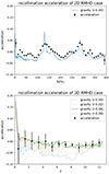 |
Fig. A.1. Axial distribution of the acceleration by effective gravity at the jet boundary for 2D RMHD case MHD1-2D (top) and 3D RMHD case MHD1 (bottom). Different color lines indicate the effective gravity at different radii of simulations, R = Rjb (blue dotted), Rjb − 0.02 (orange dotted), Rjb − 0.04 (green solid), and Rjb − 0.06, where Rjb is the radius of the jet boundary. Star marks are the azimuthal averaged radial acceleration calculated directly from the radius variations. The error bar is the standard deviation of the averages. |
Appendix B: Effect of the boundary condition
Since the jet in our simulation is over-pressured than the external medium, not in equilibrium, we apply a sharp boundary between jet and external medium to make it expand freely when simulation starts. However, as discussed by Abolmasov & Bromberg (2023), for example, such sharp boundary would produce numerical noise and thus introduce spurious effects. In order to test it, we perform simulations with a smooth boundary through the approach developed by Abolmasov & Bromberg (2023). Here, we choose ΔR = 0.04Rj so that we can achieve a smooth boundary transition in 0.2Rj.
Figure B.1 shows 2D axial distribution of logarithmic density for HD and MHD1 cases with two different boundary conditions, sharp boundary (a,c) and smooth boundary (b,d). In hydrodynamic case (left two panels), these two different boundary scenarios are mostly similar except that the size of the recollimation structure. In the smooth boundary case, it is a little smaller than that with a sharp boundary. However, RTI is triggered in both cases. For the MHD1 case (right two panels), the conclusion is the same. Smooth boundary relieves the disruption of jet but RTI and CD kink instability still evolve.
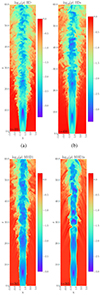 |
Fig. B.1. 2D axial distributions of logarithmic density for sharp boundary (a, c) and smooth boundary (b, d) for HD case (top two panels) at ts = 400 and MHD1 case (bottom two panels) at ts = 365. |
In summary, boundary conditions do not affect the main results qualitatively.
Appendix C: A higher jet Lorentz factor
The bulk Lorentz factor in this work is fixed to a moderate value of 3. Here we explore the impact of a larger Lorentz factor of jets with γj = 10 in the MHD1 case, as commonly adopted for blazars. Due to increase of jet Lorentz factor, the effective inertia of the jet becomes 11 times higher than that in the original MHD1 case. We expect recollimation to be slower and on a smaller scale.
As is shown in Figure C.1 shows 2D axial distribution of logarithmic density of higher jet Lorentz factor case. As we expected, large effective inertia slows down the growth of instability, and therefore the jet propagate for a longer distance stability that is consistent with the simulation of Tchekhovskoy & Bromberg (2016).
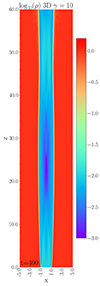 |
Fig. C.1. Axial distribution of logarithmic density for MHD1 with higher jet Lorentz factor, γ = 10 at ts = 400. |
For a rough estimation, we treat the recollimation approximation as an oscillation. We obtain the length of a recollimation structure  . The length in the MHD1 case is around 14 and in the higher jet Lorentz factor case is 49. We confirm that 49/14 ≃ 10/3 is ratio of the initial jet Lorentz factor.
All Tables
Basic properties of the different cases, where ⟨σ⟩ is the averaged magnetization.
All Figures
|
Fig. 1. Initial distributions of toroidal fields (the left panel) and magnetizations (the right panel) for various cases. |
| In the text | |
|
Fig. 2. Distribution of the logarithmic density (left), effective inertia, I = γ2ρh + Bz2 + Bϕ2 (middle), and magnetic pitch (right) for the 2D RMHD model MHD1-2D at ts = 400. |
| In the text | |
|
Fig. 3. 2D axial distribution of logarithmic density (a), effective inertia, I = γ2ρh (b), and the Lorentz factor (c) for the 3D RHD case HD at ts = 400. |
| In the text | |
|
Fig. 4. Distribution on the xy plane of density (left) and the Lorentz factor (right) at z = 15 Rj (top) and z = 30 Rj (bottom) for the HD case at ts = 400. |
| In the text | |
|
Fig. 5. 2D axial distribution of logarithmic density (a), effective inertia (b), magnetic pitch (c), magnetization (d), and the Lorentz factor (e) for the 3D RMHD case MHD1 at ts = 365. |
| In the text | |
|
Fig. 6. Distribution on the xy plane of density and the Lorentz factor at z = 15 Rj (top) and z = 30 Rj (bottom) for the MHD1 case at ts = 365. |
| In the text | |
|
Fig. 7. Time evolution of averaged radial velocity |vr|/c at z = 60 Rj with the cases of 3D RHD (HD, red), 2D RMHD (MHD1-2D, dashed yellow), and 3D RMHD (MHD1, blue). |
| In the text | |
|
Fig. 8. 2D axial distribution of the logarithmic density for the cases of different magnetic pitches and magnetic strength at ts = 400. (a) Higher magnetic pitch case (MHD2) with k = 1 and P = 0.50, (b) lower magnetic pitch case (MHD3) with |
| In the text | |
|
Fig. 9. Same as Fig. 7 but for cases with different magnetic pitches. The green line represents the higher magnetic pith case MHD2 (k = 1 and P = 0.5) and the purple line indicates the lower magnetic pitch case MHD3 case ( |
| In the text | |
|
Fig. 10. Distributions on the xy plane of effective inertia at z = 12 Rj (the left panel) and z = 13 Rj (the right panel) for the MHD1 case at ts = 365. |
| In the text | |
|
Fig. 11. 3D density isosurface at t = 360. The white (blue) surface marks the isosurface where density equals 0.01(0.005). The yellow lines are traces of the magnetic field lines. The color scales with the logarithm of the density. |
| In the text | |
|
Fig. 12. Azimuthal average density profiles at R = 1 Rj for ts = 397 (dash-dotted blue), 398 (dashed orange), 399 (dotted green), and 400 (solid red). |
| In the text | |
|
Fig. A.1. Axial distribution of the acceleration by effective gravity at the jet boundary for 2D RMHD case MHD1-2D (top) and 3D RMHD case MHD1 (bottom). Different color lines indicate the effective gravity at different radii of simulations, R = Rjb (blue dotted), Rjb − 0.02 (orange dotted), Rjb − 0.04 (green solid), and Rjb − 0.06, where Rjb is the radius of the jet boundary. Star marks are the azimuthal averaged radial acceleration calculated directly from the radius variations. The error bar is the standard deviation of the averages. |
| In the text | |
|
Fig. B.1. 2D axial distributions of logarithmic density for sharp boundary (a, c) and smooth boundary (b, d) for HD case (top two panels) at ts = 400 and MHD1 case (bottom two panels) at ts = 365. |
| In the text | |
|
Fig. C.1. Axial distribution of logarithmic density for MHD1 with higher jet Lorentz factor, γ = 10 at ts = 400. |
| In the text | |
Current usage metrics show cumulative count of Article Views (full-text article views including HTML views, PDF and ePub downloads, according to the available data) and Abstracts Views on Vision4Press platform.
Data correspond to usage on the plateform after 2015. The current usage metrics is available 48-96 hours after online publication and is updated daily on week days.
Initial download of the metrics may take a while.