| Issue |
A&A
Volume 609, January 2018
|
|
|---|---|---|
| Article Number | A73 | |
| Number of page(s) | 12 | |
| Section | The Sun | |
| DOI | https://doi.org/10.1051/0004-6361/201629828 | |
| Published online | 10 January 2018 | |
Structure of sunspot light bridges in the chromosphere and transition region
1 Instituto de Astrofísica de Canarias (IAC), Vía Lactéa, 38200 La Laguna (Tenerife), Spain
e-mail: This email address is being protected from spambots. You need JavaScript enabled to view it.
2 Departamento de Astrofísica, Universidad de La Laguna, 38205 La Laguna (Tenerife), Spain
Received: 2 October 2016
Accepted: 6 September 2017
Abstract
Context. Light bridges (LBs) are elongated structures with enhanced intensity embedded in sunspot umbra and pores.
Aims. We studied the properties of a sample of 60 LBs observed with the Interface Region Imaging Spectrograph (IRIS).
Methods. Using IRIS near- and far-ultraviolet spectra, we measured the line intensity, width, and Doppler shift; followed traces of LBs in the chromosphere and transition region (TR); and compared LB parameters with umbra and quiet Sun.
Results. There is a systematic emission enhancement in LBs compared to nearby umbra from the photosphere up to the TR. Light bridges are systematically displaced toward the solar limb at higher layers: the amount of the displacement at one solar radius compares well with the typical height of the chromosphere and TR. The intensity of the LB sample compared to the umbra sample peaks at the middle/upper chromosphere where they are almost permanently bright. Spectral lines emerging from the LBs are broader than the nearby umbra. The systematic redshift of the Si iv line in the LB sample is reduced compared to the quiet Sun sample. We found a significant correlation between the line width of ions arising at temperatures from 3 × 10⁴ to 1.5 × 10⁵ K as there is also a strong spatial correlation among the line and continuum intensities. In addition, the intensity−line width relation holds for all spectral lines in this study. The correlations indicate that the cool and hot plasma in LBs are coupled.
Conclusions. Light bridges comprise multi-temperature and multi-disciplinary structures extending up to the TR. Diverse heating sources supply the energy and momentum to different layers, resulting in distinct dynamics in the photosphere, chromosphere, and TR.
Key words: Sun: chromosphere / Sun: transition region / sunspots
© ESO, 2018
1. Introduction
Sunspots are manifestations of high concentrations of magnetic flux in the solar photosphere. They live up to several months, orders of magnitude longer than a convection timescale (≈10–20 min). Sunspots are structured in a dark umbra surrounded by a penumbra. The magnetic field lines are close to vertical in an umbra and close to horizontal in a penumbra. Larger umbra are typically darker and show higher magnetic field strength (Bray & Loughhead 1964; McIntosh 1981). Two magnetic configurations are discussed for sunspots: a monolithic flux tube and a cluster of flux tubes (Parker 1979; Spruit 1981). The formation of sunspots have not often been observed due to the short timescale of the formation process compared to the lifetime of sunspots (Schlichenmaier et al. 2010; Shimizu et al. 2012). Sunspot properties are summarized in several review papers (Solanki 2003; Moradi et al. 2010; Rempel & Schlichenmaier 2011; Borrero & Ichimoto 2011).
Sunspot umbra have an average intensity of ≈ 60% in the near-infrared and ≈ 1% in the near-ultraviolet (UV) continuum, in units of the average quiet Sun intensity. Sunspot umbra usually consist of a dark umbral core, light bridge(s), and umbral dots. Light bridges (LBs) are elongated regions with enhanced intensities compared to nearby umbra. They either split an umbra or are embedded in the umbra. Muller (1979) categorized LBs based on their photospheric continuum intensities: photospheric, penumbral, or umbral. From previous observations, it is known that LBs generally have a weaker magnetic field strength and a more horizontal field orientation than nearby umbra (Lites et al. 1991; Wiehr & Degenhardt 1993; Leka 1997; Jurčák et al. 2006; Felipe et al. 2016).
Light bridges show transient brightenings in higher atmospheric layers during the formation and decay of sunspots (Zwaan 1992, Shimizu et al. 2009; Rezaei et al. 2012). They have either a segmented or a filamentary morphology (Lites et al. 2004). They are observed to form through the continuation of penumbra filaments into the umbra (Katsukawa et al. 2007). Light bridges can also form as trapped granules by the coalescence of pores during the formation and growth of sunspots. These LBs can reappear during the decay of a sunspot (Vázquez 1973; García de La Rosa 1987). Signs of the overturning convection are observed in LBs, leading observers to conclude that the convection is the main energy transport mechanism in LBs (Rimmele 1997, 2008; Rouppe van der Voort et al. 2010; Lagg et al. 2014). Thermodynamic properties of the LBs in pores are reported by Hirzberger et al. (2002), Giordano et al. (2008), and Sobotka et al. (2013). In his numerical simulation, Rempel (2011) found a LB associated with deep structures reaching down to the bottom of the simulation domain (>10 Mm). In some high-resolution observations, a dark lane was observed in LBs (Sobotka et al. 1993; Berger & Berdyugina 2003), which was reproduced in a simulation of an emerging active region by Cheung et al. (2010).
Anomalous, unidirectional, or bidirectional (shear) flows are observed in LBs (Berger & Berdyugina 2003; Schleicher et al. 2003;Rimmele 2008; Louis et al. 2009; Rouppe van der Voort et al. 2010; Schlichenmaier et al. 2012; Bello González et al. 2012). The chromospheric activity of LBs are observed in the line-core images of the Ca ii H and Hα lines (Shimizu et al. 2009; Robustini et al. 2016). In Ca ii filtergrams, LBs show small-scale jets of several arcseconds moving away from the LB (Louis et al. 2014; Beck et al. 2015). Hα surges have also been observed associated with LBs (Canfield et al. 1996; Asai et al. 2001; Tziotziou et al. 2005).
Partially ionized plasma in the chromosphere and transition region (TR) is usually investigated through the UV spectrum of diverse ionized atoms forming at a temperature range of 4 ≤ log T [K] ≤ 6. The NASA Interface Region Imaging Spectrograph (IRIS) is a small telescope launched on June 27, 2013, that observes the Sun in the UV part of the spectrum (IRIS; De Pontieu et al. 2014b). IRIS records spectral lines forming at a range of temperature and heights that spans the photosphere up to the middle of the TR. In the near-UV, IRIS observes a spectral range around the two strong Mg ii lines at 280 nm and their nearby continuum, while the far-UV spectra includes several strong emission lines originating in the solar TR (133–141 nm). Compared to the Solar Ultraviolet Measurements of Emitted Radiation (SUMER, Wilhelm et al. 1995), IRIS records a restricted spectral range with a higher spatial and spectral resolution and with four UV slitjaw channels.
The temperature rise above the photosphere is accompanied by an increase in the nonthermal (turbulence) velocity. Profiles of the chromospheric and TR lines have been analyzed to measure the temperature and nonthermal velocities as well as the electron density (Tandberg-Hanssen 1960; Kjeldseth Moe & Nicolas 1977; Lemaire 2007). The TR lines usually show some degree of asymmetry as well as a large line width far in excess of their thermal broadening. The deviation of the wing intensities of TR lines from a single Gaussian cannot be explained in terms of the damping since the electron densities are not high enough. Multi-component models are required to fit the average quiet Sun line profiles, indicating an inhomogeneous structure of the solar TR (Peter 2000, 2010). Mariska (1992) reviews the solar TR while Aschwanden (2004) summarizes the relevant techniques and physical processes in the TR and corona.
IRIS observations.
In this paper, we study the mere existence and physical properties of light bridges in the solar chromosphere and transition region and try to establish a connection between the intensity enhancements in different layers. Currently a cusp-shape magnetic configuration is supported by photospheric observations of LBs (Leka 1997; Jurčák et al. 2006; Lagg et al. 2014; Felipe et al. 2016). In the cusp model, the umbral field lines wrap around the nonmagnetic or weak field light bridge and merge in the upper photosphere (Jurčák et al. 2006, their Fig. 7). These magnetic field lines cannot be differentiated from umbral fields in the higher layers. Therefore, we do not expect to find trace of LBs in the chromosphere and TR (similar to umbral dots). In other words, the existence of significant LB signals in the upper atmosphere indicates a systematic effect, and challenges the cusp model. Compiling a large sample of LBs, we collected evidence of the presence of a LB signal in the upper atmosphere. To this end we observed 40 sunspots with IRIS including 60 LBs. Using IRIS data which is free from seeing and differential refraction effects, we studied LB images in the photosphere, chromosphere, and TR. The paper has the following structure. We review the observed datasets and briefly discuss the analysis methods in Sect. 2. The sample of 42 k LB pixels gathered from the observed LBs allows us to evaluate the line and continuum intensities, the line width and the Doppler shifts. The distribution of these parameters, the correlations among them, and a comparison of the LB sample with the umbra and quiet Sun samples are addressed in Sect. 3. Discussion and conclusions are presented in Sects. 4 and 5, respectively. A follow-up paper will address IRIS slitjaws and magnetic properties of the light bridges.
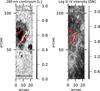 |
Fig. 1 IRIS maps of observation #10 in Table 1. The left panel displays the photospheric continuum map normalized to the average quiet Sun intensity. Theright panel shows the logarithm of the intensity of the Si iv 140.3 nm line measured with a Gaussian fit (see Sect. 2.2 for more details). The 280 nm and silicon masks of the two LBs are marked on the corresponding panels. Both maps were clipped for a better visibility. The widths of the LBs are comparable in the photosphere and the TR. We note the relative shift of the LBs in the two maps. The solar limb is toward the left. |
2. Observations and data analysis
Table1 lists properties of IRIS sunspot scans. Our sample of 40 sunspots observed between 2013 and 2016 comprises 60 LBs. The integration time varies from 5 to 32 s, leading to a substantial difference in the signal-to-noise ratios among different datasets. All intensities discussed through the paper (except the one in Fig. 1) are normalized by the integration time to make a comparison possible. Each map was analyzed in the full slit length; we have the two hair lines in the analyzed parameters and use them to align the data in different spectral channels (Fig. 1). In the following, we only discuss spectral lines that are present in all the scans in our sample.
All observed spectra except for the 280 nm band were subject to a median filtering and a convolution with a small Gaussian kernel to reduce the effect of noise, which is particularly important when dealing with a low-amplitude signal like that in the O i 135.56 nm line. Cosmic rays (CRs) are corrected on two-dimensional rasters after masking spectral lines. Whenever a line was hit by a CR, the amplitude was compared to similar lines to discriminate between a strong signal and a CR. The method was conservative, so the low-amplitude CRs pass through this filter, and we did not modify spectral lines when it was not necessary.
We created three masks for each LB using an intensity threshold: the continuum at the 280 nm, the Mg ii k line core, and the Si iv core intensities. The sum of the magnesium and silicon masks constructed an overall mask for each LB. The intensity threshold for the 280 nm mask was set to 0.1 Ic, where Ic stands for the average quiet Sun intensity. For the silicon mask, the threshold was set to 3 DN (Fig. 1). For the O i and C ii lines, the overall mask was used. We gathered analyzed data from all LBs inside the masks, resulting in 42 436 entries for each line parameter. Sample IRIS maps with two LBs are shown in Fig. 1. As seen in this example, the width of the LBs in the photosphere and the TR are similar (LBs do not expand exponentially with height). In the following, we discuss statistics of the line intensity, the line width, and the Doppler shift in this sample that includes all individual pixels in our LBs. To facilitate a comparison of the LB sample with quiet Sun and umbra, we created two extra samples. These two statistical ensembles consist of a large fraction of quiet Sun/umbra regions in our IRIS observations. The umbra sample does not include penumbral grains or LBs but consists of bright and dark umbra (umbral flashes). There are more entries in the quiet Sun and umbra samples than in the LB sample (2 502 255 and 194 783, respectively). The pixel size of IRIS spectral rasters in the far-UV (near-UV) is 0.33 (0.4)′′, while the slit width is 0.33′′ (De Pontieu et al. 2014b).
2.1. Near-ultraviolet spectrum
The near-Ultraviolet (NUV) spectrograph records a spectral range around the Mg ii h and k lines and two quasicontinuum windows in the 280 nm range. The spectral dispersion in the NUV channel was either 2.544 or 5.088 pm corresponding to a velocity dispersion of 2.7 or 5.5 km s-1 per pixel, respectively. The velocity modulations due to the orbital motion of the satellite was corrected for using a strong photospheric line in the 280 nm channel (Fe i 283.2435 nm). To this end, we calculated the average line-core position along each slit. The average spectral position as a function of time was then fitted with a polynomial to make sure that the residual systematic variation is below the expected uncertainty of the velocity calibration. When a systematic trend was clear along the slit (particularly for observations with the full slit length of 175′′ far from the disk center), a linear fit was used to correct for this spectral gradient. For a velocity calibration in the photosphere, we assumed the average quiet Sun velocity to be zero, leading to a systematic error of less than 1 km s-1, which is small compared to the velocity dispersion.
Atomic parameters of selected spectral lines.
2.2. Far ultraviolet spectrum
The far-Ultraviolet (FUV) spectrograph often records four wavelength bands: the C ii lines at 133.6 nm; the O i and C i lines at 135.6 nm; the Si iv line at 139.3 nm; and the O iv line at 140.1 nm and the Si iv line at 140.3 nm. The chromospheric O i line at 135.56 nm forms at a temperature range of 7–16 × 103 K, comparable to the formation temperature of the Mg ii k line. The O i 135.56 nm and the C i 135.584 nm lines are fitted together. The O i line is used to construct a velocity modulation curve to correct for the orbital motion of the satellite in the FUV channel (the procedure is identical to the NUV case). The C ii line pair, the Si iv lines, and the O iv lines form in the TR.Although the C ii ionization fraction peaks at 2.5 × 10⁴ K (Rathore & Carlsson 2015), the Si iv 140.277 nm line forms at log T [K] ≈ 4.8 (Peter 2001) and the O iv lines form at log T [K] ≈ 5.4 (Arnaud & Rothenflug 1985,their Table V). Table 2 lists the formation temperature, rest wavelength, and excitation potential of selected spectral lines in the IRIS spectra. While the C ii line pair are often optically thick, the Si iv and O iv lines only show the double reversal pattern in flaring regions, for example. From the two Si iv lines, we only discuss the Si iv 140.277 nm line in this paper as the Si iv 139.376 nm line is blended with a Ni ii line and is not always recorded. A spectral synthesis of these lines (using CHIANTI, Landi et al. 2013) shows that the C ii, the Si iv, and the O iv lines form at a limited temperature range. The spectral dispersion in the FUV channel was either 1.296 or 2.592 pm corresponding to a velocity dispersion of 2.8 or 5.6 km s-1 per pixel, respectively.
Data analysis:
we developed a new data reduction package for the IRIS spectra that analyzes the major spectral lines (Rezaei 2017). The program1 was tested on a variety of datasets and is available in the SolarSoft (Freeland & Handy 1998). For the NUV data, it performs a spectral analysis and a Gaussian fit to the core of the Mg ii h and k lines and a few nearby lines. For the FUV spectral channels, a multi-line Gaussian fit is performed. Details of the fitting procedure is explained in the following. In the fit procedure the observational errors, which are a joint action of the photon and thermal noise, are taken into account. We used the hairlines to align the NUV and FUV data (Fig. 1).
2.3. Near-ultraviolet data
We define the standard parameters of double-reversal profiles of the Mg ii h and k lines in a similar way to the Ca ii H and K lines (Cram & Damé 1983; Lites et al. 1993; Rezaei et al. 2007; Beck et al. 2008). The core of the Mg ii h and k lines forms higher than the Ca ii H and K lines, due to a larger opacity (Leenaarts et al. 2013a). While the k1 minima form at about the temperature minimum, the k2 and k3 form above 1 Mm (Leenaarts et al. 2013b). At first we fit a single-Gaussian function to the Mg ii h and k lines between k1 (h1) minima after removing the wing slope. After that, we proceed with a double- and a triple-Gaussian fit. A guided multi-Gaussian fitting method was previously presented by several authors (Peter 2000; Tian et al. 2011). In this approach, the result of each step is used to construct an initial guess for the next step that incorporates a more complex model. We use the Mpfit package for the Gaussian fits discussed in this paper (Markwardt 2009).
2.4. The FUV data
We used a multi-line multi-Gaussian fitting approach to simultaneously fit all spectral lines between 139 and 141 nm listed in Table 2. The fitting procedure is similar to the Mg ii case where we gradually increased the number of the free parameters to have a better fit and evaluate the results using the reduced chi-square (Bevington & Robinson 1992). The same technique was used to fit the O i 135.56 nm and C ii 133.45 nm lines. The O i 135.56 nm line forms at a height of about 1.0–1.5 Mm and is always optically thin (Lin & Carlsson 2015). The C i 135.58 nm line in the red wing of the O i line is usually weaker, but can be stronger in flares (Cheng et al. 1980). For the Si iv 140.3 nm line, we also performed a double-Gaussian fit. The two Gaussians do not have similar properties: one has a larger amplitude, a narrower line, and a smaller shift (core component), while the other usually has a smaller amplitude, a broader line, and a larger shift (tail component). The core and tail components retrieved during this process are discussed in Sect. 4.2.
The UV continuum at 135 nm forms beyond the temperature minimum (Judge 2006). To estimate the UV continuum, we computed the median of a subset of continuum windows excluding the 1% outliers, which was then used as an initial guess in the Gaussian fits. This resulted in a fairly clean continuum map but sometimes there are a few warm or hot pixels. There is an offset between the upper and lower halves of the chip. This offset is due to simultaneous readout of two cameras and is present in some datasets. In addition in some datasets, the dark subtraction in the calibration procedure creates a negative UV continuum in the level 2 data. We correct the negative continuum values in the maps by lifting the lower limit of the continuum distribution to have a positive minimum. A new IRIS technical document will address these issues.
Unlike photospheric spectral lines which have a well-known convective blueshift pattern and have an average velocity in quiet Sun areas close to zero (Doerr 2015), the average quiet Sun TR line profiles show significant Doppler shifts (Peter & Judge 1999). For the Si iv line, we compared the line positions with the mean position of the S i 140.151 nm line (assuming this line to be at rest), while for the C ii line the nearby Ni ii 133.520 nm was used as a reference, again assuming that the mean profile of this line has zero Doppler shift. The accuracy of these assumptions is about 1–2 km s-1.
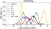 |
Fig. 2 Histograms of the line and continuum intensities in the LB sample. Intensities are normalized to the integration time. The core intensity of the Mg ii k line is denoted k3. The LB sample includes 42 436 entries from 60 LBs. We used 100 bins in all histograms. |
3. Results
The analysis of 60 LBs resulted in a sample of several NUV and FUV line parameters. The LB sample consists of 42 436 entries for each parameter. In the following, we mainly discuss the peak intensity, the line width, and the velocity of the Mg ii k, O i, C ii, and Si iv lines. Light bridges are clearly seen in the core of the Mg ii k and Si iv lines. While the IRIS scanning slit clearly leaves the pattern of umbral flashes in the maps of the magnesium line core, the Mg ii k3 intensities do not show umbral flashes in the LBs.
Figure 2 shows distributions of the continuum and line intensities in the LB sample. It is seen that LBs have highest intensity in the Mg ii k line, an order of magnitude higher than the corresponding 280 nm continuum. The median LB intensity in the 280 nm continuum and the Mg ii k line (k3) are 23.1 and 306.4 DN s-1, respectively. Excluding 5% outliers in the histograms, a probability interval covering 90% of all entries for the 280 nm and the Mg ii k line corresponds to [6.4, 72.6] and [97.0, 752.5] DN s-1, respectively. The O i 135.560 nm line has a median intensity of 0.7 DN s-1 with a 90% probability interval of [0.2, 3.9] DN s-1, which is comparable to the O iv 140.115 nm forbidden line with an average amplitude of 0.2 DN s-1 and a 90% probability interval of [0.0, 1.2] DN s-1. The ratio of the line-core intensity of the C i 135.58 and O i 135.56 nm lines is distinctly different in the LB sample than in the quiet Sun sample. Excluding all pixels that do not have a clear signal in both lines, the median ratio in the LB sample is about 0.5, while it is 0.3 in the quiet Sun sample. The intensities of the C ii and Si iv lines are 5.8 and 1.3 DN s-1, respectively, about an order of magnitude higher than the O i and the O iv lines. The 90% probability interval of the C ii line corresponds to [0.8, 42.1] DN s-1, of the same order of magnitude as the Si iv range ([0.2, 23.0] DN s-1). For a double-Gaussian fit to the Si iv line, the core and tail components have a median intensity of 1.3 and 0.2 DN s-1, respectively. The UV continuum can be measured in the 133, 135, or 140 nm wavelength range, and the resulting maps are fairly comparable. The UV continuum discussed below is retrieved from the 135 nm wavelength range. It has the smallest intensity consistent with the fact that all the studied FUV lines are in emission: the UV continuum has a median intensity of 0.2 DN s-1 with a 90% probability interval of [0.0, 0.3] DN s-1.
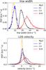 |
Fig. 3 Histograms of the line widths (top) and velocity (bottom) in the LB sample. The line width is equal to 2σ where σ is the Gaussian width. For a description of the velocity calibration, see Sect. 2.2. Positive velocity corresponds to downflow. |
 |
Fig. 4 Two-dimensional density plots of the intensity parameters in the FUV and NUV spectra. Color bars denote the density of points. The h1 intensity and the line-core intensity of the subordinate Mg ii 297.80 nm line are the result of a profile analysis while the rest are retrieved from the Gaussian fits. A positive correlation is seen in all panels. |
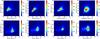 |
Fig. 5 Two-dimensional density plots of the line widths (W = 2σ) in different lines. There is a correlation between the width of the FUV lines (C ii, Si iv, O iv), while there is no significant correlation between the chromospheric and the FUV lines. |
The top panel of Fig. 3 shows the line width distribution in the LB sample. The line width is measured at 1 /e of the peak intensity and is equal to 2σ, where σ is the Gaussian width. The line width of the O i and Mg ii k lines (mean of the k2 emission widths) are comparable (8.4 and 10.6 km s-1), as was expected since these lines mainly form in a similar temperature range. The O i line width of 90% of all entries in the LB sample falls between [4.0, 14.5] km s-1, which spans a broader range than the Mg ii k2 range ([5.6, 11.8] km s-1). The C ii line has a median width of 18.0 km s-1 and the 90% probability interval was [13.0, 32.2] km s-1. The single-Gaussian fit to the Si iv line has a median width of 22.0 km s-1 and the 90% probability interval covers a broader range than the C ii line ([13.4, 44.9] km s-1). Applying a double-Gaussian fit, the core and tail components have a median width of 20.0 and 29.8 km s-1 and the corresponding 90% probability intervals are [12.9, 40.1] and [12.8, 85.8] km s-1, respectively. A single-Gaussian fit to the O iv 140.115 nm line (Table 2) yields a median width of 25.3 km s-1 and the 90% probability interval corresponds to [15.8, 45.1] km s-1. The extreme largest line widths resemble flaring regions. The FUV observed lines are significantly wider than the sound speed at the corresponding formation temperature (4.3 km s-1 for the C ii and Si iv lines, Peter 2001). Distribution of the velocity in the LB sample is shown in the bottom panel of Fig. 3. Light bridges are redshifted, almost in all spectral lines. The blueshifts in the O i and Mg ii lines are comparable to the redshifts. The median velocity in these two lines are 1.3 and 0.4 km s-1, and the 90% probability intervals correspond to [−4.1, 5.7 ] and [−3.1, 2.7 ] km s-1, respectively. The C ii line is systematically redshifted (2.0 km s-1) with a 90% probability interval of [−3.2, 8.7 ] km s-1. The Si iv line has the largest redshift and 90% probability interval (4.3, [−9.1, 22.9 ] km s-1).
Figure 4 shows two-dimensional density plots of the line intensities in the NUV and FUV spectra. From the 280 nm photospheric continuum to the O iv line core, there is a significant spatial correlation between all pairs of the line and continuum intensities. Noteworthy is the fact that even the UV continuum and the subordinate Mg ii 279.80 nm line-core intensity which have weak signals clearly show the correlation to the other lines. In most panels, the parameters on either axis were retrieved from the analysis of a different spectral band.
Density plots of the line width (at 1 /e of the peak amplitude) for all lines in our study are shown in Fig. 5. The width of the C ii line has a significant correlation only with the Si iv and O iv lines. The width of the k2 peaks corresponds to the average width of the two Gaussians used to fit the line and does not represent the distance of the two emission peaks. The Mg ii k2 width does not scale with the width of the FUV lines. The same is true for the width of the O i line (Fig. 5, bottom panels): the width of these two lines changes in a restricted range. The tail toward the very small line width in the O i panels is perhaps due to noise. The density plot of the Mg ii k line versus the O iv line (not shown here) is very similar to that for the Si iv line (top right panel). In summary, we found evidence of a correlation between the width of the TR lines while there is no significant correlation between the width of the TR and chromospheric lines.
 |
Fig. 7 Two-dimensional density plots of the logarithm of the line intensity versus the line width. |
Density plots of the Doppler shifts are shown in Fig. 6. All lines are dominated by redshifts, which is also clear in the velocity histograms (Fig. 3, bottom panel). The velocity of the Si iv and C ii lines span a much broader range than the chromospheric lines. There is a significant correlation between the velocity in the Mg ii k center of gravity and the C ii lines as well as between the C ii and Si iv lines. The relation between the magnesium k3 and the silicon line-core velocities shows some trend with a large scatter. The velocity of the O i line does not clearly show a trend with other lines. There is also a positive correlation between the intensity and the line width in all the lines (Fig. 7). Although the line intensities span several orders of magnitude, the line widths changes within a factor of two. The scatter increases toward the hotter lines.
A comparison of the histograms of the LB sample with the umbra and quiet Sun samples is displayed in Fig. 8. The wing intensity of the Mg ii k line in quiet Sun is brighter than the LBs and umbra (panels A). The same is true for the continuum intensity at the 280 nm (not shown here). As seen in panels B−D, LBs are one order of magnitude brighter than umbra in the Mg ii k line. In panels D–G, the LBs are brighter than the quiet Sun in the Mg ii k, O i, C ii, and Si iv lines. The intensity enhancement compared to umbra in the TR lines is smaller than the Mg ii k line (panels E–H). A comparison of the line width is shown in panels I–L. Light bridge profiles are either significantly wider than umbra (Mg ii k and C ii lines, panels I and J) or have an extended tail toward very broad lines (panels K and L). Although LBs are dominated by redshifts, the velocity distribution are blueshifted in the LBs and umbra samples compared to the quiet Sun sample (panels O and P). The chromospheric velocities of our LBs shown in panels M and N are close to umbra.
Light bridges are systematically displaced in different spectral lines such that high forming lines are closer to the solar limb. To estimate this projection effect, we used the 280 nm continuum, the Mg ii k, and the Si iv masks to find the center of mass of the LBs in different channels. The displacement along the radial direction was then compared to the distance to the disk center (Fig. 9). The displacement and the x coordinate have opposite signs so a LB is closer to the disk center in the photosphere than in the TR. The amount of the displacement at one solar radius in the Mg ii k/Si iv maps is about 2.0/3.5 Mm which corresponds to the formation height of the chromosphere/TR. The deviations compared to the linear fit can be due to a mismatch of the exact shape of the LBs, its extension, or a real height difference between different LBs in the sample.
4. Discussion
4.1. Vertical extent
We measured a systematic displacement between the center of mass position of the LBs in the TR and chromosphere compared to the photosphere. The LBs in the photospheric continuum are closer to the disk center than in the Si iv and Mg ii maps which hints at the three-dimensional structure of LBs in the solar atmosphere. The scatter in Fig. 9 close to the disk center is significant as the absolute amount of the shift is smaller close to the disk center than close to the limb. Therefore, the measured shifts close to the disk center are more prone to the noise (the shifts are partially affected by the mismatch of the exact shape of the LBs in different layers). This displacement is partially responsible for the scatter in the density plots (Fig. 4): there is a larger scatter between two parameters that form at very different temperatures than those that form at a comparable temperature. This systematic displacement also indicates that LBs to some extent are coherent structures in an extended height range. The fact that each IRIS scan was recorded over approximately one hour does not necessarily imply that the measured emission enhancements associated with LBs should have a stationary nature. A quasi-stationary bright LB can be sustained through the transient events provided that the brightenings happen with a high enough frequency as suggested by Toriumi et al. (2015), which is consistent with observations of LBs with IRIS filtergrams reported by Bharti (2015) and Yang et al. (2015). These authors found frequent small-scale jets associated with LBs. Although there is no temporal evolution in the LB sample, our results remain qualitatively consistent with an intermittent supply of the energy and momentum to LBs.
The presence of a systematic LB signal in the chromosphere and TR is not consistent with a cups-shaped magnetic configuration (Leka 1997; Jurčák et al. 2006; Lagg et al. 2014; Felipe et al. 2016). According to this model, the field lines associated with LBs merge in the upper photosphere. Therefore, in the chromosphere and TR, the LB field lines are not distinguishable from the umbra. This is inconsistent with a systematic observation of LBs in the upper atmosphere.
 |
Fig. 8 Distribution of the intensity, line width, and velocity in the LB sample (green) compared to the umbra (black) and quiet Sun (red) samples. The quiet Sun area surrounding sunspots includes some plage regions seen as a secondary population in the photosphere (panel A). Histograms of the intensity parameters are shown in panels A–H, while panels I–L, and M–P show histograms of the line widths and velocities, respectively. The line width of Mg ii k2 shown on panel (I) marks the average width of the two Gaussians used to fit the line. All intensity parameters (panels A–H) were normalized to the corresponding integration times. Positive velocity denotes redshift. |
 |
Fig. 9 Scatter plot of the displacement between center of mass of the LBs in the 280 nm continuum channel and the Mg ii and Si iv lines. The x-axis represents the radial distance to the disk center in the heliographic coordinate. The red line shows a linear fit passing through the origin. The estimated altitude of each line as the displacement value at one solar radius is shown in each panel. |
4.2. Intensity
Light bridges show an excess intensity that can be more than one order of magnitude higher than the nearby umbra. The intensity of the UV continuum (at 135 nm) is about 0.2 DN s-1 and is significantly more prone to noise than line-core intensities. While not true in all cases, there are many LBs in which the UV continuum maps show a pattern of the photospheric LB. The UV continuum at 135 mm mimics the local heatings at ≳ 0.5 Mm. We also note that the subordinate Mg ii 279.80 nm line in the red wing of the Mg ii k line shows emission in several LBs, distinct from the observed absorption line in the photosphere and plage (Carlsson et al. 2015). These findings provide evidence for an energy deposit in the low chromosphere.
The blue wing of the Mg ii k line (Fig. 8, panel A) has a similar intensity distribution to that of the 280 nm continuum (Fig. 2). The magnesium k2 and k3 bands have an intensity that is higher than the co-spatial and co-temporal continuum by more than one order of magnitude (Fig. 8, panels C and D), which indicates that the radiative processes cannot provide enough energy and there must be some sort of chromospheric heating that sustains the Mg ii k line-core emission. The asymmetry between the violet and red emission peaks in the LBs is comparable to quiet Sun (k2v is slightly stronger than k2r). The emission strength, the ratio between the k2v and k3, is between umbra and quiet Sun. Unlike nearby umbral profiles which have a single lobe, LB profiles show the typical double-reversal pattern, while sometimes the two lobes merge and form a very asymmetric line profile. The Mg ii k line profiles are distinctly different from that in an umbra or a plage: the lines are broader than umbra, but not as broad as plage (particularly not as broad in the k1 level). The line width remains comparable to quiet Sun, although it is usually smaller. This has two implications: First, the LB temperature stratification in a one-dimensional model atmosphere should significantly deviate from an umbral (or a plage) atmospheres. Second, the umbral scattered light does not play an important role in LB profiles as there is a clear distinction between the LB and umbra profiles (umbra profiles are narrower, have a single emission peak, and have an intensity up to three orders of magnitude smaller than LB profiles). The strong correlation between the intensity in different continuum and lines is comparable to quiet Sun areas (Doschek et al. 2004). Our results remain consistent with Chae et al. (1998), who suggested that the lower to mid TR comprises coherent structures.
As discussed by Peter (2000, 2010), many spectral lines in the TR including the Si iv 140.3 nm line show a tail component in the network regions while a single-Gaussian fit is enough to fit the observed profile in inter-network. The double-Gaussian fit of our LBs (Sect. 2.4) resulted in an average tail component that is about 14% of the total intensity (tail plus core). Peter (2001) studied the core and tail components in quiet Sun network and reported a similar fraction (14.8%). The average line width measured in our LBs are, however, significantly smaller than that reported by Peter (2001) for networks (22/20/30 vs. 28/25/44 km s-1 for the single-Gaussian, and the core and tail components of the double Gaussian). The higher spatial resolution of IRIS data compared to SUMER implies that the difference can be partially due to the instrumental effects (a line profile emerging from a larger resolution element has a larger width due to the velocity dispersion compared to that originating from a smaller area). Further studies of networks using IRIS data facilitates a more accurate comparison.
Yang et al. (2015) found LB traces in the IRIS 133 nm slitjaw images co-temporal and co-spatial with high-resolution TiO filtergrams from ground-based observations. IRIS filtergrams at 133 and 140 nm have a mixed contribution from the core and continuum of the FUV lines. Unlike photospheric and chromospheric filtergrams in the visible/near-infrared in which spectral line-core intensities are within a factor 2–10 of the nearby continuum, a line-core intensity in the UV lines can be a factor of 104 higher than the nearby continuum. Therefore, even if the continuum wavelength range covers a band that is hundred times larger than the width of the strong FUV line in the filter passband (0.4 nm for the Mg ii filter and 4 nm for the 133/140 nm filters, De Pontieu et al. 2014b), the contribution of the line to the integrated filtergram signal can exceed that from the UV continuum by a large factor. As a result, in active regions, the line mostly outweights the continuum signal in the IRIS filtergrams, while in quiet Sun the filtergrams represent the UV continuum. In contrast, the line intensities from IRIS spectra presented here have no contribution from the line wing or nearby continuum. Similarly, the UV continuum in our data shows a pure continuum signal that is not contaminated through the wings of spectral lines. This distinction is absent in the IRIS filtergrams of LBs presented by Yang et al. (2015) and Bharti (2015).
4.3. Line width
The line widths in the chromosphere and TR are primarily nonthermal as the turbulence velocity increases toward the upper umbra atmosphere (Kneer & Mattig 1978; Lites & Skumanich 1982); they are also nonthermal in a quiet Sun atmosphere (Vernazza et al. 1981). As seen in Fig. 3, the line width increases with the formation temperature, which is in accordance with the general understanding that the maximum nonthermal broadening happens at about 3 × 10⁵ K in quiet Sun, beyond the temperature range discussed here (Dere & Mason 1993; Peter 2001). The increased broadening of the chromospheric and TR lines in the LBs compared to umbra provides evidence for an energy deposit in the atmosphere. Among different line broadening mechanisms, we note a few of them relevant to the discussed spectral lines. A line can be broadened by the turbulence in the atmosphere (Rutten 2003), by a velocity dispersion due to unresolved structures in the resolution element (Feldman 1983), or − as discussed by De Pontieu et al. (2014a)− by a twisting motion of small-scale flux elements.
The k2 width of the Mg ii k line in LBs is larger than umbra but comparable to quiet Sun (Fig. 8, panel I). This is in contrast to the width of the O iv 140.115 nm lines which shows a similar distribution for the umbra, LB, and quiet Sun, although the LB and quiet Sun samples have a larger tail toward larger line widths (panel L). The situations in the Si iv and C ii lines are different: while the LB distribution peaks close to the quiet Sun sample for the former, it peaks close to the umbra sample for the latter (panels J and K). Distribution of the width of the C ii line in quiet Sun and sunspot presented here are in agreement with Rathore et al. (2015). In both cases, the line width is the result of fitting a single-Gaussian function. That the C ii line width in LBs is more comparable to umbra is consistent with our finding that the contrast of LBs in this line are not as large as in the Mg ii k and Si iv lines (panels D, F and G). As discussed by Avrett & Loeser (2008) and Rathore & Carlsson (2015), the formation of the C ii line pair and also the background opacity in the 133 nm wavelength range should be treated in nonlocal thermodynamic equilibrium. Three-dimensional effects produce a C ii line profile that is significantly influenced by nearby regions (Rathore & Carlsson 2015, their Fig. 10). The net effect is that we observe LBs that are less distinct in the C ii line than they are in the Mg ii k and Si iv lines.
We found evidence for a spatial correlation between the logarithm of the intensity and the line width in LBs in all of the lines in this study (Fig. 7). Our finding is in agreement with Dere & Mason (1993) who found significant correlation between the Si iv intensity and line width in quiet Sun. Peter (2000) reported a similar correlation in the networks. A comparable relation between the intensity and line width was obtained by Lemaire et al. (1999) for coronal holes and for quiet Sun. Akiyama et al. (2005) also found a line width−intensity spatial correlation for a set of TR spectral lines in quiet Sun. They did not find a clear correlation for the Si iv line in quiet Sun while there is a correlation in our LB sample.
In our statistical ensemble of LBs, the line width of the simultaneously observed FUV lines show a spatial correlation (Fig. 5). The relation between the line width of the C ii, Si iv, and O iv lines indicates that there is a correlation between plasma in this range of temperatures (3 × 10⁴ to 1.5 × 10⁵ K) in a LB atmosphere. This is not fully consistent with the idea of a one-dimensional stratification in which different temperatures occupy different heights, unless one assumes that there is a coherent structure which extends over a few Mm. Our results do not support a stationary bright wall; unlike the Mg ii k line, the UV continuum − and to a minor extent weak FUV lines − do not show the LB pattern in all cases. If there were a bright wall (hotter than the nearby umbra) from the photosphere to the TR, the UV continuum would show the LBs in all cases. Supporting a solid bright wall is further complicated considering the vast dynamics of LBs in the photosphere and chromosphere. Furthermore, there is an ample amount of fine structure in the chromosphere and TR of LBs, which has a small scale down to the resolution element. We interpret the correlations as a signature of a multi-component TR. The fine structure in LBs and indications of a multi-component atmosphere support an inhomogeneous TR discussed by Peter (2001).
4.4. Doppler shifts
Light bridges in the TR show both redshift and blueshift, although the redshift is dominant. Only in the strong photospheric line of the Fe i 283.2435 nm and the chromospheric lines of Mg ii k and O i 135.560 nm, are the blue- and red-shifts comparable (Fig. 8, panels M and N). The range of the measured velocities significantly increases with the formation temperature of the FUV lines. The median redshift in the Si iv line in the quiet Sun sample (7.3 km s-1) is larger than the corresponding value in the LB and umbra samples (4.4 and 2.4 km s-1, respectively). The average quiet Sun redshift in the sample is slightly larger than the typical average quiet Sun velocities reported for this line (Peter & Judge 1999), but this can be due to selection effects as the quiet Sun sample is not very quiet. The quiet Sun sample is often in the moat around sunspots. The C ii velocity distribution in the quiet Sun sample (panels O) has a median value at 2.3 km s-1, while the corresponding velocity for the LB/umbra sample is 2/1.8 km s-1.
The Doppler shifts of the Mg ii k, C ii, and Si iv lines show a positive correlation while the O i line-core velocity does not show a clear trend with other lines (Fig. 6). As mentioned earlier, the O i line is weaker than the C ii and Si iv lines and hence is more prone to noise. The correlation between the Doppler shifts is in accordance with the correlations between the line widths and the line intensity discussed above. The coupling between the cool and hot plasma is essential in the heating processes. In the cool plasma there are many neutrals, while the bulk of the TR consists of ionized atoms. Recent numerical models hint at the importance of the ambipolar diffusion in the plasma heating in the chromosphere where hydrogen and helium are partially ionized (Khomenko et al. 2014; Martínez-Sykora et al. 2015). Altogether, we found evidence for a physical state in LBs where cool and hot plasma mutually influence each other and their spatial variation shows some degree of coherence. We conclude that LBs consists of multi-component (multi-thermal) atmospheres.
4.5. Energy balance
IRIS observations of LBs have revealed enhanced emission compared to nearby umbra from the photosphere to the chromosphere and TR. Although the bulk of LBs are brighter or much brighter than nearby umbra in all lines, there are some LBs that are not significantly brighter in one or more lines, in particular in the weak O i and the UV continuum. In other words, there is an intrinsic diversity in the contrast of LBs in the FUV emission lines, while they are always distinctly brighter in the Mg ii k line. This perhaps indicates that different energy sources govern the cool and hot lines (see below). This reminds us of the variation in the continuum contrast of LBs in the photosphere as discussed by Schlichenmaier et al. (2016). Further investigations are required to find out how far the amount of energy deposited in the chromosphere and TR depends on the photospheric structure and dynamics. Photospheric observations provide evidence for overturning convection in LBs (Rimmele 2008; Rouppe van der Voort et al. 2010). A convectively driven LB is also supported by the numerical simulations of Cheung et al. (2010) and Rempel (2011). These simulations do not extend beyond the temperature minimum and so cannot be directly compared with our results. Even if LBs show a close resemblance to quiet Sun in the photosphere, our results prove that their properties notably deviate from quiet Sun in the chromosphere and TR. As a result, extra heating mechanisms are required to explain their excess emission in addition to those operating in quiet Sun.
The intensity of spectral lines and continuums in LBs compared to quiet Sun varies in the atmosphere. Although LBs are usually not as bright as granulation in the photosphere, they are significantly brighter in the Mg ii k line and at the same time only slightly brighter in the O i line. The O i line forms at a height of 1.0–1.5 Mm (Lin & Carlsson 2015) while the magnesium line has contributions from layers up to several Mm above the solar surface. In other words, the contrast of LBs compared to quiet Sun increases from photospheric continuum up to a height of about 2.0–2.5 Mm where the k3 forms (Leenaarts et al. 2013b). The contrast does not further increase upward for the C ii and Si iv lines and at the same time there is little difference between the LB and quiet Sun in the O iv line (Fig. 8). If the energy flow were primarily from the corona toward the chromosphere as suggested by the downflow in the TR lines, one would expect to find a larger relative intensity in the TR than in the chromosphere. Our findings support an energy deposit which peaks in the middle/upper chromosphere.
Oscillations are prevalent in the solar atmosphere. Umbral flashes are oscillations observed in the chromosphere of sunspot umbra (Socas-Navarro et al. 2000). Maps of the chromospheric intensities do not show the umbral flashes in LBs. We used IRIS time series to estimate importance of the mechanical heating. To this end, we performed a Fourier analysis of a 2h fixed-slit time series for entries 15 and 16 in Table 1. A comparison of the Fourier power in the LB and umbra reveals that while umbral flashes have a typical frequency higher than 5 mHz, the power in LBs peaks at frequencies lower than 5 mHz both in the intensity and velocity of the Mg ii k line. This agrees with the fact that we do not find signs of umbral flashes in LBs. Similar results were reported by Zhang et al. (2017), who observed different oscillation frequencies in LBs and umbra. Yurchyshyn et al. (2015) found strong power concentration associated with a LB using a 100 min IRIS time series. These findings are comparable to those of Sobotka et al. (2013) who measured the acoustic power of LBs in the photosphere. In summary, the oscillation period of LBs observed in the Mg ii k line is between three and five minutes. There is also a significant power concentration observed associated with LBs. Therefore, dissipation of the mechanical energy contributes to the chromospheric energy balance of LBs.
It is not clear whether the spectral lines discussed here are supplied by a common heating mechanism or experience diverse heating regimes. The strong dependence of the longitudinal thermal conductivity on the temperature (T5/2, Stix 2002) implies that the thermal conduction is not efficient for a generic chromospheric temperature of 104 K. The situation changes toward the upper chromosphere where the temperature and the temperature gradient increase substantially. The conducted heat flux is concentrated in channels of strong magnetic field strength. As seen in Fig. 1, the width of the LBs in the TR is comparable to the one in the photosphere, although the pressure and density between the two layers are different by several orders of magnitude. In other words, LBs do not exponentially expand with height as they are surrounded by strong magnetic field of umbra. Furthermore, we do not observe peripheral intensity enhancements in LB maps of the TR lines: the heating should happen through the volume of the LB and not over its boundary. It is feasible to perceive that an efficient thermal conduction in the Si iv and O iv lines contributes to the heating of LBs. An exponentially increasing density with depth along with an inefficient thermal conductivity at low temperatures prevents the thermal conduction from playing an important role in the low chromosphere.
In quiet Sun, the upper chromosphere and TR lines form above the β = 1 surface, i.e., in a highly conductive media in which the magnetic pressure dominates the gas pressure (the plasma-β is the ratio of the thermal pressure to the magnetic pressure, Aschwanden 2004). In sunspot umbra, the surface of equipartition between magnetic and thermal energy density is located at a lower geometrical height than the quiet Sun. Metcalf et al. (1995) found that in a sunspot, the magnetic field becomes force-free in the low chromosphere. In contrast, Socas-Navarro (2005) observed a sunspot with a spectropolarimeter in the photosphere and chromosphere and found that the magnetic field was not force-free up to ≈ 2 Mm. A LB perhaps further complicates the magnetic field structure and the field deviates from a potential configuration. We tried to roughly estimate the plasma-β in LBs assuming a field strength of ≈ 1 kG and a thermodynamic stratification similar to model-M of Maltby et al. (1986). The plasma-β is smaller than unity for layers at log τ ≈ −4 and above. In addition, the convective motion in LBs builds up a magnetic free energy (Peter et al. 2004). Rezaei et al. (2012) discussed evolution of a forming sunspot and its impact on the magnetic field structure of a LB. Robustini et al. (2016) found magnetic reconnection as the driving force of the small-scale jets in the LBs. We conclude that currents should be abundant in LBs. At present, there are many reports of significant current in the photosphere (Jurčák et al. 2006; Felipe et al. 2016) and a few in the chromosphere (Tritschler et al. 2008). In summary, the Joule heating contributes to the emission enhancements in the LBs, which is consistent with our finding that the median intensity ratio of the C i 135.58 nm and O i 135.56 nm lines is about 0.5 in LBs compared to ≈ 0.3 in quiet Sun. The ratio was interpreted as a tracer of flaring activity by Cheng et al. (1980). To further quantify the importance of the magnetic, mechanical, or thermal conduction energy, the field strength and oscillations have to be measured simultaneously. In particular, high-resolution ground observations help to distinguish if segmented or filamentary LBs harbor different heating mechanisms.
5. Conclusion
We studied a sample of light bridges (LBs) observed with IRIS to address their presence and properties in the chromosphere and transition region. The strength of the emission lines varies among LBs and also depends on the selected spectral line. Light bridges have a clear signature in the Mg ii k and Si iv lines. The correlations between the line widths and the intensities of spectral lines originating from plasma at different temperatures implies an inhomogeneous and multi-thermal state that deviates from a typical quiet Sun and umbra atmosphere. This is further fortified by strong correlations between the intensity of different lines. Considering the small-scale structure of LBs, the spatial distribution, and the diversity in the emission enhancements, light bridges are multi-thermal, dynamic, and coherent structures in the solar atmosphere from the photosphere to the transition region. The observed emission enhancements in the chromosphere and transition region compiles evidence against the cusp-shape magnetic structure of LBs. The variation in the emission enhancements in different layers indicates that different heating mechanisms operate in the atmosphere.
It is also available at http://github.com/reza35/mosic
Acknowledgments
IRIS is a NASA small explorer mission developed and operated by LMSAL with mission operations executed at NASA Ames Research center and major contributions to downlink communications funded by the Norwegian Space Center (NSC, Norway) through an ESA PRODEX contract. The author gratefully acknowledges support from the Spanish Ministry of Economy and Competitivity through project AYA2014-60476-P (Solar Magnetometry in the Era of Large Solar Telescopes). Part of this work was supported by the DFG grant RE 3282/1-2. This work has made use of the VALD database, operated at Uppsala University, the Institute of Astronomy RAS in Moscow, and the University of Vienna. We would like to thank the referee for the constructive suggestions.
References
- Akiyama, S., Doschek, G. A., & Mariska, J. T. 2005, ApJ, 623, 540 [NASA ADS] [CrossRef] [Google Scholar]
- Arnaud, M., & Rothenflug, R. 1985, A&AS, 60, 425 [NASA ADS] [Google Scholar]
- Asai, A., Ishii, T. T., & Kurokawa, H. 2001, ApJ, 555, L65 [NASA ADS] [CrossRef] [Google Scholar]
- Aschwanden, M. J. 2004, Physics of the Solar Corona. An Introduction (Praxis Publishing Ltd) [Google Scholar]
- Avrett, E. H., & Loeser, R. 2008, ApJS, 175, 229 [NASA ADS] [CrossRef] [Google Scholar]
- Beck, C., Schmidt, W., Rezaei, R., & Rammacher, W. 2008, A&A, 479, 213 [NASA ADS] [CrossRef] [EDP Sciences] [Google Scholar]
- Beck, C., Choudhary, D. P., Rezaei, R., & Louis, R. E. 2015, ApJ, 798, 100 [NASA ADS] [CrossRef] [Google Scholar]
- Bello González, N., Kneer, F., & Schlichenmaier, R. 2012, A&A, 538, A62 [NASA ADS] [CrossRef] [EDP Sciences] [Google Scholar]
- Berger, T. E., & Berdyugina, S. V. 2003, ApJ, 589, L117 [NASA ADS] [CrossRef] [Google Scholar]
- Bevington, P. R., & Robinson, D. K. 1992, Data reduction and error analysis for the physical sciences, 2nd edn. (McGraw-Hill) [Google Scholar]
- Bharti, L. 2015, MNRAS, 452, L16 [NASA ADS] [CrossRef] [Google Scholar]
- Borrero, J. M., & Ichimoto, K. 2011, Liv. Rev. Sol. Phys., 8, 4 [Google Scholar]
- Bray, R. J., & Loughhead, R. E. 1964, Sunspots (London: Chapman Hall) [Google Scholar]
- Canfield, R. C., Reardon, K. P., Leka, K. D., et al. 1996, ApJ, 464, 1016 [NASA ADS] [CrossRef] [Google Scholar]
- Carlsson, M., Leenaarts, J., & De Pontieu, B. 2015, ApJ, 809, L30 [NASA ADS] [CrossRef] [Google Scholar]
- Chae, J., Schühle, U., & Lemaire, P. 1998, ApJ, 505, 957 [CrossRef] [Google Scholar]
- Cheng, C. C., Feldman, U., & Doschek, G. A. 1980, A&A, 86, 377 [NASA ADS] [Google Scholar]
- Cheung, M. C. M., Rempel, M., Title, A. M., & Schüssler, M. 2010, ApJ, 720, 233 [NASA ADS] [CrossRef] [Google Scholar]
- Cram, L. E., & Damé, L. 1983, ApJ, 272, 355 [NASA ADS] [CrossRef] [Google Scholar]
- De Pontieu, B., Rouppe van der Voort, L., McIntosh, S. W., et al. 2014a, Science, 346, 1255732 [CrossRef] [Google Scholar]
- De Pontieu, B., Title, A. M., Lemen, J. R., et al. 2014b, Sol. Phys., 289, 2733 [NASA ADS] [CrossRef] [Google Scholar]
- Dere, K. P., & Mason, H. E. 1993, Sol. Phys., 144, 217 [NASA ADS] [CrossRef] [Google Scholar]
- Doerr, H.-P. 2015, Ph.D. Thesis, University of Freiburg [Google Scholar]
- Doschek, G. A., Mariska, J. T., & Akiyama, S. 2004, ApJ, 609, 1153 [NASA ADS] [CrossRef] [Google Scholar]
- Feldman, U. 1983, ApJ, 275, 367 [NASA ADS] [CrossRef] [Google Scholar]
- Felipe, T., Collados, M., Khomenko, E., et al. 2016, A&A, 596, A59 [NASA ADS] [CrossRef] [EDP Sciences] [Google Scholar]
- Freeland, S. L., & Handy, B. N. 1998, Sol. Phys., 182, 497 [NASA ADS] [CrossRef] [Google Scholar]
- García de La Rosa, J. I. 1987, Sol. Phys., 112, 49 [NASA ADS] [CrossRef] [Google Scholar]
- Giordano, S., Berrilli, F., Del Moro, D., & Penza, V. 2008, A&A, 489, 747 [NASA ADS] [CrossRef] [EDP Sciences] [Google Scholar]
- Hirzberger, J., Bonet, J. A., Sobotka, M., Vázquez, M., & Hanslmeier, A. 2002, A&A, 383, 275 [NASA ADS] [CrossRef] [EDP Sciences] [Google Scholar]
- Judge, P. 2006, in Solar MHD Theory and Observations: A High Spatial Resolution Perspective, eds. J. Leibacher, R. F. Stein, & H. Uitenbroek, ASP Conf. Ser., 354, 259 [Google Scholar]
- Jurčák, J., Martínez Pillet, V., & Sobotka, M. 2006, A&A, 453, 1079 [NASA ADS] [CrossRef] [EDP Sciences] [Google Scholar]
- Katsukawa, Y., Yokoyama, T., Berger, T. E., et al. 2007, PASJ, 59, 577 [Google Scholar]
- Kaufman, V. 1982, Phys. Scr., 26, 439 [NASA ADS] [CrossRef] [Google Scholar]
- Khomenko, E., Collados, M., Díaz, A., & Vitas, N. 2014, Phys. Plasmas, 21, 092901 [NASA ADS] [CrossRef] [Google Scholar]
- Kjeldseth Moe, O., & Nicolas, K. R. 1977, ApJ, 211, 579 [NASA ADS] [CrossRef] [EDP Sciences] [Google Scholar]
- Kneer, F., & Mattig, W. 1978, A&A, 65, 17 [NASA ADS] [Google Scholar]
- Kramida, A., Ralchenko, Y., Reader, J., & and NIST ASD Team. 2015, NIST Atomic Spectra Database (ver. 5.3), [Online], http://physics.nist.gov/asd. National Institute of Standards and Technology, Gaithersburg, MD [Google Scholar]
- Kupka, F., Piskunov, N., Ryabchikova, T. A., Stempels, H. C., & Weiss, W. W. 1999, A&AS, 138, 119 [NASA ADS] [CrossRef] [EDP Sciences] [MathSciNet] [PubMed] [Google Scholar]
- Kurucz, R. L. 2003, Robert L. Kurucz on-line database of observed and predicted atomic transitions [Google Scholar]
- Kurucz, R. L. 2011, Robert L. Kurucz on-line database of observed and predicted atomic transitions [Google Scholar]
- Lagg, A., Solanki, S. K., van Noort, M., & Danilovic, S. 2014, A&A, 568, A60 [NASA ADS] [CrossRef] [EDP Sciences] [Google Scholar]
- Landi, E., Young, P. R., Dere, K. P., Del Zanna, G., & Mason, H. E. 2013, ApJ, 763, 86 [NASA ADS] [CrossRef] [Google Scholar]
- Leenaarts, J., Pereira, T. M. D., Carlsson, M., Uitenbroek, H., & De Pontieu, B. 2013a, ApJ, 772, 89 [NASA ADS] [CrossRef] [Google Scholar]
- Leenaarts, J., Pereira, T. M. D., Carlsson, M., Uitenbroek, H., & De Pontieu, B. 2013b, ApJ, 772, 90 [NASA ADS] [CrossRef] [Google Scholar]
- Leka, K. D. 1997, ApJ, 484, 900 [NASA ADS] [CrossRef] [Google Scholar]
- Lemaire, P. 2007, Adv. Space Res., 39, 1876 [NASA ADS] [CrossRef] [Google Scholar]
- Lemaire, P., Bocchialini, K., Aletti, V., Hassler, D., & Wilhelm, K. 1999, Space Sci. Rev., 87, 249 [NASA ADS] [CrossRef] [Google Scholar]
- Lin, H.-H., & Carlsson, M. 2015, ApJ, 813, 34 [NASA ADS] [CrossRef] [Google Scholar]
- Lites, B. W., & Skumanich, A. 1982, ApJS, 49, 293 [NASA ADS] [CrossRef] [Google Scholar]
- Lites, B. W., Bida, T., Johannesson, T., & Scharmer, G. B. 1991, ApJ, 373, 683 [NASA ADS] [CrossRef] [Google Scholar]
- Lites, B. W., Rutten, R. J., & Kalkofen, W. 1993, ApJ, 414, 345 [NASA ADS] [CrossRef] [Google Scholar]
- Lites, B. W., Scharmer, G. B., Berger, T. E., & Title, A. M. 2004, Sol. Phys., 221, 65 [NASA ADS] [CrossRef] [Google Scholar]
- Louis, R. E., Bellot Rubio, L. R., Mathew, S. K., & Venkatakrishnan, P. 2009, ApJ, 704, L29 [NASA ADS] [CrossRef] [Google Scholar]
- Louis, R. E., Beck, C., & Ichimoto, K. 2014, A&A, 567, A96 [NASA ADS] [CrossRef] [EDP Sciences] [Google Scholar]
- Maltby, P., Avrett, E. H., Carlsson, M., et al. 1986, ApJ, 306, 284 [Google Scholar]
- Mariska, J. T. 1992, The solar transition region (New York: Cambridge Astrophysics Series) [Google Scholar]
- Markwardt, C. B. 2009, in Astronomical Data Analysis Software and Systems XVIII, eds. D. A. Bohlender, D. Durand, & P. Dowler, ASP Conf. Ser., 411, 251 [Google Scholar]
- Martínez-Sykora, J., De Pontieu, B., Hansteen, V., & Carlsson, M. 2015, Philosophical Transactions of the Royal Society of London Series A, 373, 20140268 [Google Scholar]
- McIntosh, P. S. 1981, in The Physics of Sunspots, eds. L. E. Cram, & J. H. Thomas, 7 [Google Scholar]
- Meggers, W. F., Corliss, C. H., & Scribner, B. F. 1975, Tables of Spectral-Line Intensities, Part I – Arranged by Elements, Part II – Arranged by Wavelengths, Natl. Bur. Stand. Monograph 145 (U.S. Nat. Bur. Stand.) [Google Scholar]
- Metcalf, T. R., Jiao, L., McClymont, A. N., Canfield, R. C., & Uitenbroek, H. 1995, ApJ, 439, 474 [NASA ADS] [CrossRef] [Google Scholar]
- Moore, C. E. 1970, in Nat. Stand. Ref. Data Ser., NSRDS-NBS 3 (Sect. 3) (U.S. Nat. Bur. Stand.) [Google Scholar]
- Moore, C. E. 1993, in CRC Series in Evaluated Data in Atomic Physics, ed. J. W. Gallagher (Boca Raton, FL: CRC Press) [Google Scholar]
- Moradi, H., Baldner, C., Birch, A. C., et al. 2010, Sol. Phys., 267, 1 [NASA ADS] [CrossRef] [Google Scholar]
- Muller, R. 1979, Sol. Phys., 61, 297 [NASA ADS] [CrossRef] [Google Scholar]
- Nave, G., Johansson, S., Learner, R. C. M., Thorne, A. P., & Brault, J. W. 1994, ApJS, 94, 221 [NASA ADS] [CrossRef] [Google Scholar]
- Parker, E. N. 1979, ApJ, 230, 905 [NASA ADS] [CrossRef] [Google Scholar]
- Peter, H. 2000, A&A, 360, 761 [NASA ADS] [Google Scholar]
- Peter, H. 2001, A&A, 374, 1108 [NASA ADS] [CrossRef] [EDP Sciences] [Google Scholar]
- Peter, H. 2010, A&A, 521, A51 [NASA ADS] [CrossRef] [EDP Sciences] [Google Scholar]
- Peter, H., & Judge, P. G. 1999, ApJ, 522, 1148 [NASA ADS] [CrossRef] [Google Scholar]
- Peter, H., Gudiksen, B. V., & Nordlund, Å. 2004, ApJ, 617, L85 [NASA ADS] [CrossRef] [Google Scholar]
- Rathore, B., & Carlsson, M. 2015, ApJ, 811, 80 [NASA ADS] [CrossRef] [Google Scholar]
- Rathore, B., Pereira, T. M. D., Carlsson, M., & De Pontieu, B. 2015, ApJ, 814, 70 [NASA ADS] [CrossRef] [Google Scholar]
- Rempel, M. 2011, ApJ, 729, 5 [NASA ADS] [CrossRef] [Google Scholar]
- Rempel, M., & Schlichenmaier, R. 2011, Liv. Rev. Sol. Phys., 8, 3 [Google Scholar]
- Rezaei, R. 2017, ArXiv e-prints [arXiv:1701.04421] [Google Scholar]
- Rezaei, R., Schlichenmaier, R., Beck, C., Bruls, J., & Schmidt, W. 2007, A&A, 466, 1131 [NASA ADS] [CrossRef] [EDP Sciences] [Google Scholar]
- Rezaei, R., Bello González, N., & Schlichenmaier, R. 2012, A&A, 537, A19 [NASA ADS] [CrossRef] [EDP Sciences] [Google Scholar]
- Rimmele, T. R. 1997, ApJ, 490, 458 [NASA ADS] [CrossRef] [Google Scholar]
- Rimmele, T. R. 2008, ApJ, 672, 684 [NASA ADS] [CrossRef] [Google Scholar]
- Risberg, P. 1955, Ark. Fys. (Stockholm), 9, 483 [Google Scholar]
- Robustini, C., Leenaarts, J., de la Cruz Rodriguez, J., & Rouppe van der Voort, L. 2016, A&A, 590, A57 [NASA ADS] [CrossRef] [EDP Sciences] [Google Scholar]
- Rouppe van der Voort, L., Bellot Rubio, L. R., & Ortiz, A. 2010, ApJ, 718, L78 [NASA ADS] [CrossRef] [Google Scholar]
- Rutten, R. J. 2003, Radiative Transfer in Stellar Atmosphere (Sterrekundig Instutuut Utrecht, Institute of Theoretical Astrophysics, Oslo) [Google Scholar]
- Schleicher, H., Balthasar, H., & Wöhl, H. 2003, Sol. Phys., 215, 261 [NASA ADS] [CrossRef] [Google Scholar]
- Schlichenmaier, R., Rezaei, R., Bello González, N., & Waldmann, T. 2010, A&A, 512, L1 [NASA ADS] [CrossRef] [EDP Sciences] [Google Scholar]
- Schlichenmaier, R., Rezaei, R., & Bello González, N. 2012, in 4th Hinode Science Meeting: Unsolved Problems and Recent Insights, eds. L. Bellot Rubio, F. Reale, & M. Carlsson, ASP Conf. Ser., 455, 61 [Google Scholar]
- Schlichenmaier, R., von der Lühe, O., Hoch, S., et al. 2016, A&A, 596, A7 [NASA ADS] [CrossRef] [EDP Sciences] [Google Scholar]
- Shimizu, T., Katsukawa, Y., Kubo, M., et al. 2009, ApJ, 696, L66 [NASA ADS] [CrossRef] [Google Scholar]
- Shimizu, T., Ichimoto, K., & Suematsu, Y. 2012, ApJ, 747, L18 [NASA ADS] [CrossRef] [Google Scholar]
- Sobotka, M., Bonet, J. A., & Vazquez, M. 1993, ApJ, 415, 832 [NASA ADS] [CrossRef] [Google Scholar]
- Sobotka, M., Švanda, M., Jurčák, J., et al. 2013, A&A, 560, A84 [NASA ADS] [CrossRef] [EDP Sciences] [Google Scholar]
- Socas-Navarro, H. 2005, ApJ, 631, L167 [NASA ADS] [CrossRef] [Google Scholar]
- Socas-Navarro, H., Trujillo Bueno, J., & Ruiz Cobo, B. 2000, Science, 288, 1396 [NASA ADS] [CrossRef] [Google Scholar]
- Solanki, S. K. 2003, A&ARv, 11, 153 [Google Scholar]
- Spruit, H. C. 1981, A&A, 98, 155 [NASA ADS] [Google Scholar]
- Stix, M. 2002, The Sun: An Introduction, 2nd edn. (Springer-Verlag Berlin) [Google Scholar]
- Sutherland, R. S., & Dopita, M. A. 1993, ApJS, 88, 253 [NASA ADS] [CrossRef] [Google Scholar]
- Tandberg-Hanssen, E. 1960, Astrophysica Norvegica, 6, 161 [NASA ADS] [Google Scholar]
- Tian, H., McIntosh, S. W., De Pontieu, B., et al. 2011, ApJ, 738, 18 [NASA ADS] [CrossRef] [Google Scholar]
- Toresson, Y. G. 1960, Ark. Fys. (Stockholm), 17, 179 [Google Scholar]
- Toriumi, S., Katsukawa, Y., & Cheung, M. C. M. 2015, ApJ, 811, 137 [NASA ADS] [CrossRef] [Google Scholar]
- Tritschler, A., Uitenbroek, H., & Reardon, K. 2008, ApJ, 686, L45 [NASA ADS] [CrossRef] [Google Scholar]
- Tziotziou, K., Tsiropoula, G., & Sütterlin, P. 2005, A&A, 444, 265 [NASA ADS] [CrossRef] [EDP Sciences] [Google Scholar]
- Vázquez, M. 1973, Sol. Phys., 31, 377 [NASA ADS] [CrossRef] [Google Scholar]
- Vernazza, J. E., Avrett, E. H., & Loeser, R. 1981, ApJS, 45, 635 [NASA ADS] [CrossRef] [Google Scholar]
- Wiehr, E., & Degenhardt, D. 1993, A&A, 278, 584 [NASA ADS] [Google Scholar]
- Wilhelm, K., Curdt, W., Marsch, E., et al. 1995, Sol. Phys., 162, 189 [NASA ADS] [CrossRef] [Google Scholar]
- Yang, S., Zhang, J., Jiang, F., & Xiang, Y. 2015, ApJ, 804, L27 [NASA ADS] [CrossRef] [Google Scholar]
- Yurchyshyn, V., Abramenko, V., & Kilcik, A. 2015, ApJ, 798, 136 [NASA ADS] [CrossRef] [Google Scholar]
- Zhang, J., Tian, H., He, J., & Wang, L. 2017, ApJ, 838, 2 [NASA ADS] [CrossRef] [Google Scholar]
- Zwaan, C. 1992, in in NATO ASIC Proc. 375: Sunspots. Theory and Observations, eds. J. H. Thomas, & N. O. Weiss, 75 [Google Scholar]
All Tables
All Figures
|
Fig. 1 IRIS maps of observation #10 in Table 1. The left panel displays the photospheric continuum map normalized to the average quiet Sun intensity. Theright panel shows the logarithm of the intensity of the Si iv 140.3 nm line measured with a Gaussian fit (see Sect. 2.2 for more details). The 280 nm and silicon masks of the two LBs are marked on the corresponding panels. Both maps were clipped for a better visibility. The widths of the LBs are comparable in the photosphere and the TR. We note the relative shift of the LBs in the two maps. The solar limb is toward the left. |
| In the text | |
|
Fig. 2 Histograms of the line and continuum intensities in the LB sample. Intensities are normalized to the integration time. The core intensity of the Mg ii k line is denoted k3. The LB sample includes 42 436 entries from 60 LBs. We used 100 bins in all histograms. |
| In the text | |
|
Fig. 3 Histograms of the line widths (top) and velocity (bottom) in the LB sample. The line width is equal to 2σ where σ is the Gaussian width. For a description of the velocity calibration, see Sect. 2.2. Positive velocity corresponds to downflow. |
| In the text | |
|
Fig. 4 Two-dimensional density plots of the intensity parameters in the FUV and NUV spectra. Color bars denote the density of points. The h1 intensity and the line-core intensity of the subordinate Mg ii 297.80 nm line are the result of a profile analysis while the rest are retrieved from the Gaussian fits. A positive correlation is seen in all panels. |
| In the text | |
|
Fig. 5 Two-dimensional density plots of the line widths (W = 2σ) in different lines. There is a correlation between the width of the FUV lines (C ii, Si iv, O iv), while there is no significant correlation between the chromospheric and the FUV lines. |
| In the text | |
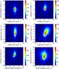 |
Fig. 6 Same as Fig. 4 but for the Doppler shifts. |
| In the text | |
|
Fig. 7 Two-dimensional density plots of the logarithm of the line intensity versus the line width. |
| In the text | |
|
Fig. 8 Distribution of the intensity, line width, and velocity in the LB sample (green) compared to the umbra (black) and quiet Sun (red) samples. The quiet Sun area surrounding sunspots includes some plage regions seen as a secondary population in the photosphere (panel A). Histograms of the intensity parameters are shown in panels A–H, while panels I–L, and M–P show histograms of the line widths and velocities, respectively. The line width of Mg ii k2 shown on panel (I) marks the average width of the two Gaussians used to fit the line. All intensity parameters (panels A–H) were normalized to the corresponding integration times. Positive velocity denotes redshift. |
| In the text | |
|
Fig. 9 Scatter plot of the displacement between center of mass of the LBs in the 280 nm continuum channel and the Mg ii and Si iv lines. The x-axis represents the radial distance to the disk center in the heliographic coordinate. The red line shows a linear fit passing through the origin. The estimated altitude of each line as the displacement value at one solar radius is shown in each panel. |
| In the text | |
Current usage metrics show cumulative count of Article Views (full-text article views including HTML views, PDF and ePub downloads, according to the available data) and Abstracts Views on Vision4Press platform.
Data correspond to usage on the plateform after 2015. The current usage metrics is available 48-96 hours after online publication and is updated daily on week days.
Initial download of the metrics may take a while.