| Issue |
A&A
Volume 608, December 2017
|
|
|---|---|---|
| Article Number | A36 | |
| Number of page(s) | 9 | |
| Section | Stellar structure and evolution | |
| DOI | https://doi.org/10.1051/0004-6361/201731323 | |
| Published online | 04 December 2017 | |
IGR J19552+0044: A new asynchronous short period polar
Filling the gap between intermediate and ordinary polars⋆
1 Universidad Nacional Autónoma de México, Instituto de Astronomia, Unidad Academica en Ensenada, 22860 Baja California, Mexico
e-mail: This email address is being protected from spambots. You need JavaScript enabled to view it.
2 Department of Physics and Astronomy, University of California, Irvine, California 92697, USA
3 Department of Physics and Astronomy, Dartmouth College, Hanover, NH 03755, USA
4 South African Astronomical Observatory, PO Box 9, Observatory 7935, Cape Town, South Africa
5 Leibniz-Institut für Astrophysik Potsdam (AIP), An der Sternwarte 16, 14482 Potsdam, Germany
6 New York University Abu Dhabi, PO Box 129188, Abu Dhabi, United Arab Emirates
7 Instituto de Física y Astronomía, Facultad de Ciencias, Universidad de Valparaíso, Av. Gran Bretaña 1111 Valparaíso, Chile
8 Center for Backyard Astrophysics (CBA), Backyard, UK
9 Departamento de Ciencias Integradas, Facultad de Ciencias Experimentales, Universidad de Huelva, 21071 Huelva, Spain
10 Department of Physics and Astronomy, University of North Carolina at Chapel Hill, Chapel Hill, NC 27599, USA
11 Department of Physics and Astronomy, University of North Carolina at Greensboro, Greensboro, NC 27402-6170, USA
Received: 7 June 2017
Accepted: 14 August 2017
Abstract
Context. Based on XMM-Newton X-ray observations IGR J19552+0044 appears to be either a pre-polar or an asynchronous polar.
Aims. We conducted follow-up optical observations to identify the sources and periods of variability precisely and to classify this X-ray source correctly.
Methods. Extensive multicolor photometric and medium- to high-resolution spectroscopy observations were performed and period search codes were applied to sort out the complex variability of the object.
Results. We found firm evidence of discording spectroscopic (81.29 ± 0.01 m) and photometric (83.599 ± 0.002 m) periods that we ascribe to the white dwarf (WD) spin period and binary orbital period, respectively. This confirms that IGR J19552+0044 is an asynchronous polar. Wavelength dependent variability and its continuously changing shape point at a cyclotron emission from a magnetic WD with a relatively low magnetic field below 20 MG.
Conclusions. The difference between the WD spin period and the binary orbital period proves that IGR J19552+0044 is a polar with the largest known degree of asynchronism (0.97 or 3%).
Key words: accretion, accretion disks / stars: magnetic field / binaries: close
Photometric and spectroscopic observational data are only available at the CDS via anonymous ftp to cdsarc.u-strasbg.fr (130.79.128.5) or via http://cdsarc.u-strasbg.fr/viz-bin/qcat?J/A+A/608/A36
© ESO, 2017
1. Introduction
AM Herculis stars, or polars, are close interacting binaries possessing white dwarfs (WD) with the strongest superficial magnetic fields among cataclysmic variables (CVs; Warner 1995). The intensity of this field varies from ~10 to 200 MG and is enough to prevent the formation of an accretion disk and channel the incoming matter from a late-type companion through the magnetic lines to the magnetic pole(s) of the WD. The WD intense magnetic field and its extended magnetosphere are thought to interact with the magnetic field of the late-type companion star and synchronize the spin period of WD with the orbital period of the binary, thereby overcoming the spin-up torque exerted by the accreting matter (Campbell 1985; King & Whitehurst 1991). A subset of CVs known as intermediate polars (IPs) or DQ Herculis stars contain WDs possessing less intense magnetic moments and these CVs do not achieve synchronization (Norton et al. 2004).
Among the subclass of polars, there are seven slightly asynchronous systems with Pspin/Porb = 1−2%. These are V1432 Aql (RXJ 1940-10), BY Cam, V1500 Cyg, CD Ind (RXJ 2115-58), and Paloma (RX J0524+42) (Campbell & Schwope 1999; Schwarz et al. 2004, 2007). Another asynchronous polar (AP) was discovered by Rea et al. (2017) while we were preparing this paper. V1432 Aql is the only AP that has a spin period longer than the orbital period, while others have Porb−Pspin ≤ 0.018 Porb (Norton et al. 2004; Pagnotta & Zurek 2016). The exact reason of the asynchronism is not known yet. Nova eruptions are considered one of the possible culprits1 (Campbell & Schwope 1999), but the efforts to find nova shells around other APs have not been successful so far (Pagnotta & Zurek 2016). It is also assumed that these systems gain synchronization relatively quickly as shown in the case of V1432 Aql (Boyd et al. 2014). Very recently, Harrison & Campbell (2016) reported that V1500 Cyg, which has been known to have large 2% disparity of its orbital (photometric) and spin (circular polarization) periods (Stockman et al. 1988), has already achieved synchronization.
Log of spectroscopic observations.
Log of photometric observations.
IGR J19552+0044 (IGR 1955+0044 hereinafter) was identified as a magnetic CV by Masetti et al. (2010) based on follow-up optical spectroscopy of hard X-ray sources detected by INTEGRAL (Bird et al. 2006). Thorstensen & Halpern (2013) obtained time series of spectroscopic and photometric data, but the coverage was insufficient to determine the period in either domain without ambiguity. Bernardini et al. (2013) studied the X-ray behavior of the object using XMM-Newton. These authors point out that IGR 1955+0044 is a highly variable X-ray source with a rather hard spectrum, showing also near-infrared and infrared variability. They inferred a high 0.77 M⊙ mass for the WD and a low accretion rate. Their period analysis was inconclusive as to whether the detected periods were orbital or spin. Based on detection of hard X-ray spectrum and multiple periodicities they proposed the AP nature for the object. We conducted follow-up spectroscopic and photometric optical observations of IGR 1955+0044. We incorporated Thorstensen & Halpern (2013) spectral observations into our study to expand the time baseline. Here we report the results of this study, deducting the binary basic parameters (e.g., spin period, orbital period, and magnetic field intensity).
Details of the observations are provided in Sect. 2. We present an analysis of the optical spectroscopy and photometry in Sect. 3. We discuss the nature of the system in Sect. 4, and conclusions are summarized in Sect. 5.
2. Observation and data reduction
The time-resolved CCD photometry and long-slit spectral observations of IGR 1955+0044 were obtained on the 0.84 m, 1.5 m and 2.1 m telescopes of the Observatorio Astronómico Nacional at San Pedro Mártir (SPM) in Mexico. On September 26, 2011 we performed simultaneous spectroscopic and UBVRI photometric observations using the 2.1 m telescope with B&Ch spectrograph and the 0.84 m with the MEXMAN filter wheel. We observed the source for three years using different combination of telescopes and instruments. The bulk of data were obtained in Bessel V, I and SDSS r, i-bands using the 0.84 m/MEXMAN and the 1.5 m/RATIR telescope/instrument, respectively. Landolt photometric stars were also observed for the absolute calibration. Exposure times were 60 s for the RATIR observations and ranged from 20 s to 90 s, depending on the filter and conditions for the 0.84 m telescope. The images were bias-corrected and flat-fielded before the differential aperture photometry was carried out. The errors of the CCD photometry were calculated from the dispersion of the magnitude of the comparison stars.
We launched the monitoring of IGR 1955+0044 using two 0.4 m robotic PROMPT telescopes located in Chile (Reichart et al. 2005). In a two month campaign from June 19 to August 7, 2013 the PROMPT telescopes were intensely employed. Most of the observations in 2013 were performed in the I filter, whereas at the beginning of June we also gathered some observations in V filter. The exposure times were 120 s throughout the campaign.
A portion of the photometric data included in this paper were obtained by observers of the Center for Backyard Astrophysics (CBA), which is a global network of telescopes devoted to the observation of cataclysmic variables (Skillman & Patterson 1993; de Miguel et al. 2016). Typical apertures are in the 0.25−0.40 m range. A total of 10 CBA observatories contributed to this campaign, providing 480 h of time-series photometry. Most of the data was unfiltered, with exposure times ranging from 45 to 60 s.
Additionally, we obtained high time resolution photometry (0.25–3 s integrations) of IGR 1955+0044 without filter (in white light). We used the 1.9 m telescope of South African Astronomical Observatory (SAAO) equipped with the SHOC camera. These observations were carried out as part of a program to search and study high-frequency quasi-periodic oscillations. generated in the accretion columns in CVs.
The spectroscopic observations were conducted with the Boller and Chivens spectrograph, equipped with a 13.5 μm (2174 × 2048) Marconi E2V-4240 CCD chip, using the 2.1 m telescope. A portion of the observations were obtained with a 1200 l/mm grating to study profiles of emission lines (FWHM = 2.1 Å); some observations were made using a 300 l/mm (FWHM = 8 Å) grating to cover almost the entire optical range and study cyclotron lines. The wavelength calibration was made with an Cu-Ne-Ar arc lamp. The spectra of the object were flux calibrated using spectrophotometric standard stars observed during the same night. The low-resolution spectra were obtained with a wide slit 350 μm to improve the flux calibration of spectra taken without slit orientation along the parallactic angle.
We also included spectra with both the 2.4 m Hiltner and 1.3 m McGraw-Hill telescopes at MDM Observatory on Kitt Peak, Arizona. We used the modspec spectrograph with either the Echelle or Templeton CCD detectors. These SITe chips are identical in pixel size and therefore both yield 2.0 Å pixel-1, but the Echelle has a larger format and covers a greater spectral range. Thorstensen & Halpern (2013) give more detail on the observing and analysis procedures.
Reduction and preliminary analysis of all spectroscopic and the photometric observations from SPM were carried out using long-slit spectroscopic and aperture photometry packages available in IRAF2. The logs of observations are presented in Tables 1 and 2.
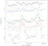 |
Fig. 1 UBVRI photometry of IGR 1955+0044. A time series (quasi-simultaneous) in all five filters during a night in September 2011 are plotted with connected filled circles. The open points were inferred from the spectrophotometry obtained at the same time by integrating flux in the portions of spectra corresponding roughly to BVR filters. Spectrophotometric measurements taken with a long slit demonstrate satisfactory flux calibration. The flux is given in ergs cm-2 s-1Å-1. |
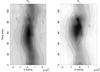 |
Fig. 2 Trailed spectra of IGR 1955+0044 centered at the Hα and Hβ are shown in the right and left panels, respectively. The bi-dimensional image is composed using 19 continuous, evenly spaced spectra obtained during about two hours on September 15, 2013. Two components are clearly visible in the right panel. The narrow component is stronger at some orbital phases. |
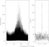 |
Fig. 3 Results of DFT period analysis of RV of emission lines. In the left panel the amplitude vs. frequency of Hβ line is presented. In the right panel the power of the same time series is presented after cleaning for alias frequencies. The maximum peak is at frequency fo = 17.22497 cycles/day. |
3. Results
3.1. Spectroscopic period and spectrophotometric characteristics
Spectra of IGR 1955+0044 were previously published by Masetti et al. (see Fig. 6 of 2010) and Thorstensen & Halpern (2013, Fig. 14). We found that the optical spectra of IGR 1955+0044 are consistent with that of a CV, but its particular classification is not simple. The object shows a standard set of hydrogen and helium lines, which are single peaked but with variable profile and intensity. A 15−25 Å FWHM of emission lines present in the λ 3800−8050 Å range is typical for CVs. The He ii line is prominent, indicating presence of a high-ionization source in the system, but its intensity is less than 1/2 Hβ. In high accretion rate polars the intensity of He ii 4686 and Hβ are often of the same order. No spectral features of the secondary star are visible in the optical spectra. The source is highly variable and intensity changes are notable by eye not only in the lines but also in the continuum and, more intriguingly, in the shape of the continuum. This variability is best demonstrated by the multicolor light curve presented in Fig. 1. It is also a better visualization of the scale and the wavelength dependency of the variability. We discuss the photometric behavior of the system in Sect. 3.2.
The trailed spectrum of the Hα line from a single night (September 15, 2013) covering the entire binary period is presented as a two-dimensional image in Fig. 2. The profiles of emission lines are complex, however, it is not possible to disentangle these profiles in most cases. Only Hα clearly shows a narrow component that can be separated from the otherwise broader line at some phases. We attempted to deblend the line with two Gaussians using the corresponding splot function in IRAF, but we could resolve two separate components in just about half of the orbital phases.
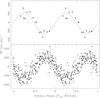 |
Fig. 4 Radial velocity curves of IGR 1955+0044. Bottom panel: single Gaussian measurements of Hβ fitted with a sine curve are shown. The filled squares are data obtained at SPM; the open squares are from MDM. Top panel: the measurement of the narrow component of the Hα line wherever we were able to distinguish it in the line profile, is shown. The sine curve with fixed period determined from the Hβ analysis was used to fit to these points. There is a small phase shift of the Hβ RV curve from being totally opposite to that of Hα. |
Hence, we used the Hβ line, as a whole, to determine the spectroscopic period based on the radial velocity (RV) variations. We chose Hβ because it is present in all observed spectra and is the most intense line. The spectral observations span more than 700 days and are comprised of blocks of several nights each with more than 300 RV measurements in total. The contribution from the narrow component in Hβ is much smaller than in Hα, which makes it suitable for the task. Therefore the RVs were measured by fitting a simple Gaussian to the line profile and using its central wavelength. A period search in the RV time series using a discrete Fourier transform (DFT) algorithm implemented in Period04 (Lenz & Breger 2005) reveals a dominant peak at 17.225 cycles/day corresponding to a 83.6 min period. The power spectrum is contaminated by aliases generated by an uneven time series and beat periods generated by multiple periodicities. The convolution of the data with the spectral window, also known as a Clean procedure (Roberts et al. 1987) reveals a single peak at the dominant frequency. The existence of this peak is also confirmed by a detection of beat periods in photometry, which we describe later on. The power and corresponding Clean spectrum are presented in Fig. 3.
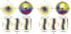 |
Fig. 5 Standard and inside-out Doppler tomography based on the Hα emission (a) and the Hβ emission (b). For each spectral line a pair of maps in the top panels show the standard tomogram (left side) and the inside-out tomogram (right side). In the bottom panel, three frames accompany maps of each line. They are comprised of the middle frame showing the observed trailed spectra with the reconstructed spectra for the standard and inside out cases to the left and right, respectively. See text for details. |
The RV curves folded with the determined period are presented in Fig. 4. The bottom panel represents the measurements of Hβ and the corresponding sinusoidal fit. There is a very wide spread of points around the best-fit sine curve. This is partially a result of a poor fit of a Gaussian to the line profile, but is also a consequence of the intrinsic velocity dispersion of the emitting gas. Usually in CVs the spectroscopic period reflects the orbital motion, but not necessarily of the stellar components, i.e the phase zero does not necessarily correspond to the binary conjunction. Assuming the tentative magnetic CV classification of IGR 1955+0044, we may find a large velocity amplitude; it would not be surprising if it exceeded 400 km s-1. The lines formed in the mass transfer stream of polars often show much higher velocity amplitudes. The other available lines were Hδ and He ii 4686, which roughly follow the same pattern as Hβ.
The object is not eclipsing, hence the orbital conjunction of stellar components is not known at this point. Measurement of RVs of the narrow component help to fetch the zero point corresponding to the inferior conjunction of the red dwarf component, assuming that IGR 1955+0044 is a magnetic CV. In such a case the narrow component originates from the irradiated face of the secondary star due to heating by the X-ray beam from the magnetic pole of the primary (Heerlein et al. 1999; Kotze et al. 2016). The RVs of the narrow component of the Hα line are presented in the top panel of Fig. 4 with the sine fit. According to calculations the +/− crossing of the rest velocity of the system corresponds to the HJD = 2 455 740.7035 ephemeris. The narrow and wide (bottom panel) components are nearly, but not exactly, in a counter phase.
The mass transfer and accretion in polars including APs takes place under strong influence of the magnetosphere of the WD and is very different from the remaining CVs (see reviews by Cropper 1990; Ferrario & Wehrse 1999). Observationally, three distinct components of emission lines were identified in polars (Schwope et al. 1997a). Not all three components are observable in every polar, which depends on the orientation of the magnetic pole, its intensity, and probably some other factors (curtaining, etc.). It is safe to say that in IGR 1955+0044 the bulk of emission is concentrated near the WD and hence, reflects the fact that the magnetically confined part of the accretion flow is the dominant source of emission lines. Careful examination of all available spectra reveals that the narrow component is visible not only in Hα, but some weak contribution can also be traced to the ballistic part of the accretion stream. This is particularly notable in the Hβ line.
Doppler tomograms, especially their inside-out projections (Kotze et al. 2016), help reveal these details. Doppler tomography in cataclysmic variables was introduced by Marsh & Horne (1988). Traditionally, filtered back-projection inversion or maximum entropy inversion were applied to translate binary-star line profiles taken at a series of orbital phases into a distribution of emission over the binary. Both these methods were primarily designed for interpretation of accretion disk CVs, where the matter is basically confined to the orbital plane. Although the maximum entropy method has also been used successfully for magnetic CVs (Marsh & Schwope 2016), part of the streams and curtains in mCVs are not in the orbital plane. Hence their interpretation in standard Doppler maps is complicated. Recently, Kotze et al. (2016) came up with the so-called inside-out projection to address magnetic CVs specifically. Here we use both, the standard and inside-out Doppler maps to demonstrate the geometry of the binary system in the velocity space.
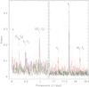 |
Fig. 6 Power spectra multiband photometry of IGR 1955+0044. The solid lines are powers after Clean procedure is applied to powers presented as dotted lines. The bluish curves are for the V band, the red are for the I band, and the green are for the WL light curves. |
Figure 5 shows the standard and the inside-out Doppler tomography based on the Hα and Hβ emission lines, respectively. The basic structure of the emission components in the observed Hα and Hβ spectra is reproduced in the reconstructed spectra from both the standard and inside-out projections. To aid the interpretation of the emission distribution in the tomograms, we overlay a model velocity profile based on arbitrary but reasonable parameters for a magnetic CV with a ~ 84 m orbital period. The primary mass was set to Mwd = 0.75M⊙ (Ferrario et al. 2015), the mass ratio was set to q = 0.13 (Knigge 2006), and the inclination angle was set to i = 65° given that the observed RV indicate a high inclination angle, yet no eclipses has been observed. The model velocity profile includes the Roche lobes of the WD (dashed line), the secondary (solid line), as well as a single particle ballistic trajectory from the L1 point up to 105° in azimuth around the WD (solid line). Magnetic dipole trajectories are calculated at 10° intervals from 5° to 105° in azimuth around the WD (thin dotted lines). The dipolar axis azimuth and co-latitude are taken to be 36° and 20°, respectively. In the Hα tomograms the emission associated with the irradiated face of the secondary is clearly visible in the position traced by the velocity profile of the secondary. This emission, however, is not isolated so clearly in the Hβ tomograms. On the other hand, in the Hβ tomograms the emission associated with the ballistic stream is more prominent and well traced by the model single particle trajectory. The most prominent feature in all the tomograms is the brighter emission in their lower halves. From the model velocity profile we deduce that this emission may be associated with the threading region, that is to say, where the matter in the ballistic stream is picked up by the magnetosphere of the WD and is elevated above the orbital plane to channel onto the magnetic pole. This matter creates a curtain that appears to be ionized by the energetic beam of the magnetic WD. The emission from the curtain follows the model dipole trajectories toward higher velocities as it is funneled toward the magnetic pole of the WD. Effectively, the Hα and Hβ tomograms confirm the magnetic nature of the object.
The shape of spectra show spectacular transformation throughout an observing run lasting several hours. However the period of the continuum variability apparently does not coincide with the spectroscopic period determined from the RV variability. This becomes obvious after just two or three individual observational runs. Therefore, we must assess the photometric periods before returning to this discussion.
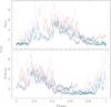 |
Fig. 7 Fast photometry. The data from three different nights (two days apart from each other) are folded with orbital (83.6 m) and spin (81.3 m) periods. Different colors indicate different nights. Strong, short variability is probably a result of magnetic “blob” accretion; no signs of WD eclipse can be found. |
3.2. Photometric variability and periods
The time-resolved photometry confirms strong variability of the object on different timescales. The simultaneous multiband photometry shows that the amplitude of the variability depends on wavelength (Fig. 1). We collected sufficient photometric data from various sources to analyze the complexity of light curves of IGR 1955+0044. Because of the difference of the amplitude of variability in different photometric bands and the underlying difference of the source of variability, the results in V, I, and white light (WL) are slightly different. The power spectra calculated by Period04 (Lenz & Breger 2005) for light curves in three observed bands (V, I, and WL) are presented in Fig. 6 by short dashed lines. The power spectra after Clean-ing to eliminate aliases created by time series are presented by solid lines of similar color. From the spectrophotometry and simultaneous multicolor photometry, we know that the largest amplitude of variability happens in the I band. Unsurprisingly, the strongest and sharpest peak is detected from I band (plotted in Fig. 6 by red color) at a 17.7 cycles per day frequency corresponding to a 81.3 m period. This matches, within statistical uncertainty, the shortest X-ray periodic signal found by Bernardini et al. (2013).
Periods detected in IGR J1955+0042.
The periodic signal is formed by a strong hump in the spectra of the object, which grows larger toward red wavelengths. We conclude that this period corresponds to the spin period of the WD and the corresponding frequency peak is denoted as fs. The one-day alias is very strong in I band, but is easily removed after deconvolution with the spectral window. Other aliases created by uneven distribution of data are also suppressed. Most of the remaining peaks in the Clean power spectrum can be identified with either the spectroscopic (orbital period) marked as fo, or sidebands formed by these two frequencies. Particularly strong are 2 × (fs−fo); (fs−fo) and 2 ∗ fs−fo. The power spectra corresponding to V and WL light curves are similar regarding the spin period, but the orbital period is not remarkable. In the V period spectrum there is a strong (fs−fo)/2 sideband frequency.
Apart from the periodic variability caused by the spin of the magnetic WD and the orbital motion, there is a huge, erratic variability that is best demonstrated by the high time resolution photometry (Fig. 7) with fast flares superimposed on a smoother, longer variability. The fast photometric light curves presented in Fig. 7 are in fluxes to demonstrate the scale of rapid variability; meanwhile light curves in the remaining figures throughout the paper are in magnitudes (i.e., logarithmic scale). While these data provide sufficient time resolution to explore the features of rapid variability, there is no adequate phase coverage to determine the orbital or spin period accurately.
The high-speed light curve folded with the orbital period in the bottom panel of Fig. 7 shows a visually better recurrence of fast-paced features than that folded with the spin period and presented in the top panel. However a dip just prior to phase 0.4 in the spin-period folded light curve may indicate a self eclipse of the weaker accreting pole. We could not identify any repetitive luminosity drop corresponding to the presence of an eclipse of stellar components in the light curves. The absence of the eclipse constrains the inclination angle of the system to i < 72deg, but provides little information otherwise. No periodic signal is detected at higher frequencies, indicating that the fast and sporadic variability is probably due to the erratic nature of the accretion flow.
The light curves folded with the Ps = 81.29 m period are presented in Fig. 8. The best defined light curve is a tide-like structure in the I band presented in the top panel. Two remarkable features of the plot are a large scatter of the points and a non-sinusoidal form of the curves. The former is not surprising since there is a huge amplitude, rapid variability around the brightness maxima revealed by the fast photometry. This is also partially due to the brightness variability on a longer timescale. The presence of two periods modulates the light curve with the beat period. Examples are provided in the top panels of Fig. 9, where the longer trend is very notable in an unfolded light curve of individual nights. That allows us not only to fit the spin period, but also to fit the trace modulation with a longer period corresponding to the f2(fs−fo) = 0.976 frequency. The amplitude of the spin period is twice as large as the longer trend. Our discussion of Figs. 8 and 9 in conjunction with the RVs and orbital modulation continues in Sect. 3.3.
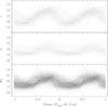 |
Fig. 8 Light curves of IGR 1955+0044 composed of all available data in the white WL, V, and I bands from bottom panel to top. |
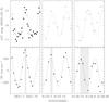 |
Fig. 9 Bottom panels: measurements of the RV of IGR 1955+0044 at three separate epochs (filled squares) with a sine fit corresponding to the fo orbital frequency. Top panels: measurements of the continuum flux in a band around 8000 Å (open squares) and I-band magnitudes (filled dots) at the same epochs. The data are fitted with a sum of sine functions with fs + 2(fs−fo) frequencies corresponding to the spin and strongest beat frequency. The shaded strips in the bottom panels denote the varying shift between phases (maximum RV vs. maximum brightness) caused by the difference of the orbital and spin frequencies. |
A signal was detected in X-rays with a 82.7 ± 1.35 m period. This period is in the middle and within the errors of two periods detected in the optical domain. The 81.3 m period, however, seems a more natural periodicity to be observed from the magnetic WD beaming collimated X-rays as it spins. The origin of the longer 101.4 m period, which was also found in the X-ray data (Bernardini et al. 2013), is not clear. It might be a sideband of the orbital period, but then other sidebands are expected to be seen, too. The X-ray observations do not provide sufficient coverage to sort out these differences or claim reality of other periods. Interestingly, the 101 m period also shows up in a least-squares periodogram (Lomb 1976) of fast photometry (not presented here). However, the DFT power spectrum shows a symmetric forest of strong lines with two basic frequencies 17.2 ± n and 17.7 ± n , where n = 1,2,3, etc. No significant signal appears around 101 m.
3.3. Footprint of diverging orbital and spin periods in the data
Figure 9 illustrates how the continuum hump appears at the different orbital phases due to the asynchronism. In the bottom three panels of Fig. 9 measurements of the RVs are presented against the photometric magnitudes (at the top panels) in three different epochs. The magnitudes are obtained from photometry when available (filled dots in the top left panel) or from the spectrophotometric fluxes converted to differential magnitudes (open squares). To obtain the latter, the spectral fluxes were integrated in a relatively narrow 60 Å intervals centered at the λ 8000 Å roughly corresponding to the I band, where the variability of the continuum is the strongest. Photometric and spectrophotometric measurements obtained at the same time are presented together in the top left panel Fig. 9. The errors of spectrophotometric measurements are difficult to assess since they depend on long-slit spectral calibration. We consider that the spectrophotometric data are in reasonable accordance with the precise photometric data. The standard deviations of both sets of data from the sine-fit are similar and are much less that the overall variability of the object.
Apparently, there is a trend in the data besides the obvious large amplitude variability, which we identified with the spin period. Hence, the curve fitted to the data is a sum of two sine functions: one with the spin frequency fs = 17.715 cycles/day and 0.85 mag amplitude and the other with the 2(fs−fo) = 0.976 cycles/day corresponding to the strongest beat frequency (see Fig. 6). The beat frequency has a smaller 0.44 mag amplitude. There is a clear displacement of the light and RV curves in the top and bottom panels from epoch to epoch. The shaded strips in each panel denote the time difference of the maximum RV occurrence to the moments of maximum brightness. The sine curve in the bottom panels has a period determined from the RV fitting and is the same as in Fig. 4. The sine curve in the top panels has a shorter period, corresponding to the spin period.
This displacement means that the observer has a constantly changing view on the magnetic pole and the magnetically controlled part of the accretion stream.
4. Discussion
4.1. Asynchronous polar interpretation
There is no doubt that the object of the study is a magnetic CV. Its periods, optical and X-ray spectral, and photometric behavior are good enough evidence for that. The spectral shape of the optical bright phase could be well interpreted as a cyclotron continuum (see the evaluation in the next section).
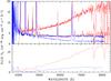 |
Fig. 10 Top panel: low-resolution spectra of IGR 1955+0044 obtained in 2011 (blue) and 2012 (red) at maximum and minimum brightness. Bottom panel: cyclotron spectra in 2011 and 2012 are shown. |
However the system is not an ordinary polar. The photometric period that we identify with the spin period of the magnetic WD is 2.8% shorter than the spectroscopic period; we think the latter reflects the orbital period of the system ( ). This is one of the extreme cases of asynchronism (Pagnotta & Zurek 2016). As a result of asynchronism the observer looks at the magnetic pole(s) under constantly changing angle with respect to the orbital phase. Also the coupling region bound to the binary frame changes its position regarding the magnetic pole (or dipoles) of the asynchronously rotating WD. Hence the intensity of accretion changes with the position angle, brightness of the system varies, and the cyclotron spectrum varies as perceived by the observer. It is demonstrated convincingly in Fig. 9. Modeling the cyclotron spectrum is a difficult task because of its ever-changing pattern.
4.2. Cyclotron spectroscopy
The pronounced brightness variability on the spin period of the WD is naturally explained in terms of cyclotron radiation from one accreting pole. The best available representative spectra at brightness maximum and minimum for the nights September 9, 2011 and July 7, 2016 were chosen to study the cyclotron contribution. These spectra are shown in Fig. 10 with blue and red colors, repectively. In 2012 the overall brightness of the source was considerably higher so that the minimum spectrum in 2012 is almost a carbon copy of the maximum spectrum from 2011. The steep rise toward long wavelength at spin-phase maximum is common to both occasions.
The difference spectrum between maximum and minimum is regarded as cyclotron spectrum and shown for the two occasions in the bottom panel of the same figure. Before subtraction the strong emissions lines were fitted with Gaussians and removed. After subtraction the resulting spectra were rebinned to 50 Å to remove the high-frequency noise as well. Some residuals due to imperfect subtraction of the asymmetric emission lines (in particular at wavelengths below 4400 Å) and the non-availability of a telluric absorption spectrum (atmospheric A-band at 7600 Å) are left in the spectra. Apart from those, the cyclotron spectra display a smooth increase toward long wavelengths. It seems as if the maximum spectral flux occurs around 8000 Å in 2011 but the spectral maximum might not be covered by the observations. In 2012 the spectral maximum seems to occur at wavelengths longer than 8000 Å.
There are no individual spectral features that could be unequivocally associated with the magnetic field in the accretion region: neither a halo Zeeman absorption line nor individual cyclotron harmonics. This fact, together with the red cyclotron spectrum, points toward a relatively low field strength. The spectral range covered by our observations then corresponds to the high-harmonic range in which individual cyclotron harmonics overlap strongly and form a quasi-continuum. If one assumes that the spectral maximum, which indicates the change from an optically thick Rayleigh Jeans to an optically thin cyclotron spectrum, occurs at 8000 Å and that this turnover corresponds to the eighth cyclotron harmonic, the implied field strength would be about 16 MG. The true field strength could be 35% lower, as argued by Schwope et al. (1997b), for the cyclotron spectrum of the AP CD Ind, which is very similar to that of IGR 1955+0044. In the abovementioned paper the cyclotron spectra of other low field polars, such as BL Hyi, EP Dra, and V393 Pav, and their similarity to that of CD Ind are presented and discussed. Further examples are EF Eri and V2301 Oph (Ferrario et al. 1995, 1996).
It appears very unlikely that the field is larger than about 20 MG. High accretion rate polars at those field strengths typically display a much bluer cyclotron spectrum (cf. MR Ser, V834 Cen Schwope et al. 1993; Schwope & Beuermann 1990) The cyclotron lines are probably shifted further down to the infrared as substantiated by large infrared excess (Fig. 10 of Bernardini et al. 2013).
4.3. Emission lines composition
The high energy beam from the magnetic pole ionizes the gas in the magnetically controlled stream, which emits the bulk of emission. A small fraction of the Hα line also originates from the irradiated face of the secondary star indicating a low temperature of the irradiation. This was demonstrated vividly by the new, inside-out tomograms (Fig. 5 top right panels). It is worth mentioning that in several polars the irradiated secondary even produces He ii. In this case the irradiation of the secondary is mild in terms of both contribution and intensity and is observed primarily in Hα.
The phasing of emission lines is appropriate to the proposed interpretation described in detail by Heerlein et al. (1999). Particularly, the narrow component of the Hα line corresponds to the top panel of Heerlein et al. (1999, Fig. 5 therein), while the broad component, which they call the accretion curtain, corresponds to their bottom panel in the figure. In the inside-out projection the crescent-shaped spot at the bottom of corresponding maps reflects the presence of that curtain, since it concurs within the area where the magnetic trajectories (black dotted lines) intercept the matter from the ballistic trajectory (red dotted lines).
The horizontal stream, or the ballistic part of the stream, is practically not visible in Hα, but becomes visible in Hβ inside-out Doppler map. It is common in polars to see either all or only some components, depending on the location of the magnetic poles and the orientation of the beam. Depending on the level of ionization it also can be seen in various species of emission lines.
Rapid photometry shows that the accretion is not smooth but is inhomogeneous and clumpy, which is today a well-established concept for polars that was proposed by Kuijpers & Pringle (1982). In the case of IGR 1955+0044 this unsteadiness of accretion flow is exaggerated by the asynchronism. However, the blobby accretion model was proposed to explain the “softness” of X-ray radiation of polars (Wickramasinghe 2014, and references therein) even though IGR 1955+0044 is rather hard source. The soft component is possibly shifted into the unobservable UV range and/or is absorbed within the systems. Actually, IPs are supposed to be harder emitters (in the X-ray), but currently many of these IPs show a soft BB component, which is a characteristic initially thought to be peculiar of polars only. Moreover, observations of polars with XMM-Newton proved that an increasing number of these objects do not show this soft emission. It is not clear why this is the case (Bernardini et al. 2012, and references therein).
5. Conclusions
We identified the INTEGRAL source IGR J19552+0044 as a new asynchronous magnetic CV or polar. Direct evidence of its magnetic nature through either Zeeman or resolved cyclotron lines or by means of (spectro-)polarimetry is outstanding. Based on optical photometric and spectroscopic observations we determined the orbital and WD spin periods of the object to be 83.6 and 81.3 min, respectively. The 2.8% rate of asynchronism is among the largest observed in a few similar objects. We only have an estimate of a moderate ≈ 16 MG field strength of the WD. This estimate agrees well with the assessment of infrared excess by Bernardini et al. (2013). Doppler tomography of emission lines confirm the small size of the WD magnetosphere, showing the accretion stream treading area all the way down the ballistic trajectory, close to the WD. Very fast photometry demonstrates large variability on very short timescales, which is consistent with the generally accepted point of view that the matter hits the magnetic pole in the form of blobs, rather than a fluid stream. The source of the spin period deviation from the orbital period in APs is not established yet and IGR J19552+0044 sheds little light on that. But the growing number of discovered APs indicate that it is not as rare as originally thought.
Among a few APs at least one (V1500 Cyg) definitely has undergone a nova explosion; this AP is also known as Nova Cygni 1975.
IRAF is distributed by the National Optical Astronomy Observatories, which are operated by the Association of Universities for Research in Astronomy, Inc., under cooperative agreement with the National Science Foundation.
Acknowledgments
G.T. and S.Z. acknowledge PAPIIT grants IN108316/IN-100617 and CONACyT grants 166376; 151858 and CAR 208512 for resources provided toward this research. J.T. acknowledges the NSF grant AST-1008217.
References
- Bernardini, F., de Martino, D., Falanga, M., et al. 2012, A&A, 542, A22 [NASA ADS] [CrossRef] [EDP Sciences] [Google Scholar]
- Bernardini, F., de Martino, D., Mukai, K., et al. 2013, MNRAS, 435, 2822 [NASA ADS] [CrossRef] [Google Scholar]
- Bird, A. J., Barlow, E. J., Bassani, L., et al. 2006, ApJ, 636, 765 [NASA ADS] [CrossRef] [EDP Sciences] [Google Scholar]
- Boyd, D., Patterson, J., Allen, W., et al. 2014, Soc. Astron. Sci. Annu. Symp., 33, 163 [NASA ADS] [Google Scholar]
- Campbell, C. G. 1985, MNRAS, 215, 509 [NASA ADS] [CrossRef] [Google Scholar]
- Campbell, C. G., & Schwope, A. D. 1999, A&A, 343, 132 [NASA ADS] [Google Scholar]
- Cropper, M. 1990, Space Sci. Rev., 54, 195 [NASA ADS] [CrossRef] [Google Scholar]
- de Miguel, E., Patterson, J., Cejudo, D., et al. 2016, MNRAS, 457, 1447 [NASA ADS] [CrossRef] [Google Scholar]
- Ferrario, L., & Wehrse, R. 1999, MNRAS, 310, 189 [NASA ADS] [CrossRef] [Google Scholar]
- Ferrario, L., Wickramasinghe, D., Bailey, J., & Buckley, D. 1995, MNRAS, 273, 17 [NASA ADS] [CrossRef] [Google Scholar]
- Ferrario, L., Bailey, J., & Wickramasinghe, D. 1996, MNRAS, 282, 218 [NASA ADS] [CrossRef] [Google Scholar]
- Ferrario, L., de Martino, D., & Gänsicke, B. T. 2015, Space Sci. Rev., 191, 111 [NASA ADS] [CrossRef] [Google Scholar]
- Harrison, T. E., & Campbell, R. K. 2016, MNRAS, submitted [Google Scholar]
- Heerlein, C., Horne, K., & Schwope, A. D. 1999, MNRAS, 304, 145 [NASA ADS] [CrossRef] [Google Scholar]
- King, A. R., & Whitehurst, R. 1991, MNRAS, 250, 152 [NASA ADS] [Google Scholar]
- Knigge, C. 2006, MNRAS, 373, 484 [NASA ADS] [CrossRef] [Google Scholar]
- Kotze, E. J., Potter, S. B., & McBride, V. A. 2016, A&A, 595, A47 [NASA ADS] [CrossRef] [EDP Sciences] [Google Scholar]
- Kuijpers, J., & Pringle, J. E. 1982, A&A, 114, L4 [NASA ADS] [Google Scholar]
- Lenz, P., & Breger, M. 2005, Commun. Asteroseismol., 146, 53 [NASA ADS] [CrossRef] [Google Scholar]
- Lomb, N. R. 1976, Ap&SS, 39, 447 [NASA ADS] [CrossRef] [Google Scholar]
- Marsh, T. R., & Horne, K. 1988, MNRAS, 235, 269 [NASA ADS] [CrossRef] [Google Scholar]
- Marsh, T. R., & Schwope, A. D. 2016, Astronomy at High Angular Resolution, 439, 195 [NASA ADS] [CrossRef] [Google Scholar]
- Masetti, N., Parisi, P., Palazzi, E., et al. 2010, A&A, 519, A96 [NASA ADS] [CrossRef] [EDP Sciences] [Google Scholar]
- Norton, A. J., Wynn, G. A., & Somerscales, R. V. 2004, ApJ, 614, 349 [NASA ADS] [CrossRef] [Google Scholar]
- Pagnotta, A., & Zurek, D. 2016, MNRAS, 458, 1833 [NASA ADS] [CrossRef] [Google Scholar]
- Rea, N., Coti Zelati, F., Esposito, P., et al. 2017, MNRAS, 471, 2902 [NASA ADS] [CrossRef] [Google Scholar]
- Reichart, D., Nysewander, M., Moran, J., et al. 2005, Nuovo Cimento C Geophysics Space Physics C, 28, 767 [Google Scholar]
- Roberts, D. H., Lehar, J., & Dreher, J. W. 1987, AJ, 93, 968 [NASA ADS] [CrossRef] [Google Scholar]
- Skillman, D. R., & Patterson, J. 1993, ApJ, 417, 298 [NASA ADS] [CrossRef] [Google Scholar]
- Schwarz, R., Schwope, A. D., Beuermann, K., et al. 1998, A&A, 338, 465 [NASA ADS] [Google Scholar]
- Schwarz, R., Schwope, A. D., Staude, A., et al. 2004, Magnetic Cataclysmic Variables, IAU Colloq., 190, 315, 230 [Google Scholar]
- Schwarz, R., Schwope, A. D., Staude, A., et al. 2007, A&A, 473, 511 [NASA ADS] [CrossRef] [EDP Sciences] [Google Scholar]
- Schwope, A. D., & Beuermann, K. 1990, A&A, 238, 173 [NASA ADS] [Google Scholar]
- Schwope, A. D., Beuermann, K., Jordan, S., & Thomas, H.-C. 1993, A&A, 278, 487 [NASA ADS] [Google Scholar]
- Schwope, A. D., Mantel, K.-H., & Horne, K. 1997a, A&A, 319, 894 [NASA ADS] [Google Scholar]
- Schwope, A. D., Buckley, D. A. H., O’Donoghue, D., et al. 1997b, A&A, 326, 195 [NASA ADS] [Google Scholar]
- Spruit, H. C. 1998, ArXiv e-prints [arXiv:astro-ph/9806141] [Google Scholar]
- Stockman, H. S., Schmidt, G. D., & Lamb, D. Q. 1988, ApJ, 332, 282 [NASA ADS] [CrossRef] [Google Scholar]
- Thorstensen, J. R., & Halpern, J. 2013, AJ, 146, 107 [NASA ADS] [CrossRef] [Google Scholar]
- Warner, B. 1995, Magnetic Cataclysmic Variables, 85, 3 [NASA ADS] [Google Scholar]
- Wickramasinghe, D. 2014, Eur. Phys. J. Web Conf., 64, 03001 [CrossRef] [EDP Sciences] [Google Scholar]
All Tables
All Figures
|
Fig. 1 UBVRI photometry of IGR 1955+0044. A time series (quasi-simultaneous) in all five filters during a night in September 2011 are plotted with connected filled circles. The open points were inferred from the spectrophotometry obtained at the same time by integrating flux in the portions of spectra corresponding roughly to BVR filters. Spectrophotometric measurements taken with a long slit demonstrate satisfactory flux calibration. The flux is given in ergs cm-2 s-1Å-1. |
| In the text | |
|
Fig. 2 Trailed spectra of IGR 1955+0044 centered at the Hα and Hβ are shown in the right and left panels, respectively. The bi-dimensional image is composed using 19 continuous, evenly spaced spectra obtained during about two hours on September 15, 2013. Two components are clearly visible in the right panel. The narrow component is stronger at some orbital phases. |
| In the text | |
|
Fig. 3 Results of DFT period analysis of RV of emission lines. In the left panel the amplitude vs. frequency of Hβ line is presented. In the right panel the power of the same time series is presented after cleaning for alias frequencies. The maximum peak is at frequency fo = 17.22497 cycles/day. |
| In the text | |
|
Fig. 4 Radial velocity curves of IGR 1955+0044. Bottom panel: single Gaussian measurements of Hβ fitted with a sine curve are shown. The filled squares are data obtained at SPM; the open squares are from MDM. Top panel: the measurement of the narrow component of the Hα line wherever we were able to distinguish it in the line profile, is shown. The sine curve with fixed period determined from the Hβ analysis was used to fit to these points. There is a small phase shift of the Hβ RV curve from being totally opposite to that of Hα. |
| In the text | |
|
Fig. 5 Standard and inside-out Doppler tomography based on the Hα emission (a) and the Hβ emission (b). For each spectral line a pair of maps in the top panels show the standard tomogram (left side) and the inside-out tomogram (right side). In the bottom panel, three frames accompany maps of each line. They are comprised of the middle frame showing the observed trailed spectra with the reconstructed spectra for the standard and inside out cases to the left and right, respectively. See text for details. |
| In the text | |
|
Fig. 6 Power spectra multiband photometry of IGR 1955+0044. The solid lines are powers after Clean procedure is applied to powers presented as dotted lines. The bluish curves are for the V band, the red are for the I band, and the green are for the WL light curves. |
| In the text | |
|
Fig. 7 Fast photometry. The data from three different nights (two days apart from each other) are folded with orbital (83.6 m) and spin (81.3 m) periods. Different colors indicate different nights. Strong, short variability is probably a result of magnetic “blob” accretion; no signs of WD eclipse can be found. |
| In the text | |
|
Fig. 8 Light curves of IGR 1955+0044 composed of all available data in the white WL, V, and I bands from bottom panel to top. |
| In the text | |
|
Fig. 9 Bottom panels: measurements of the RV of IGR 1955+0044 at three separate epochs (filled squares) with a sine fit corresponding to the fo orbital frequency. Top panels: measurements of the continuum flux in a band around 8000 Å (open squares) and I-band magnitudes (filled dots) at the same epochs. The data are fitted with a sum of sine functions with fs + 2(fs−fo) frequencies corresponding to the spin and strongest beat frequency. The shaded strips in the bottom panels denote the varying shift between phases (maximum RV vs. maximum brightness) caused by the difference of the orbital and spin frequencies. |
| In the text | |
|
Fig. 10 Top panel: low-resolution spectra of IGR 1955+0044 obtained in 2011 (blue) and 2012 (red) at maximum and minimum brightness. Bottom panel: cyclotron spectra in 2011 and 2012 are shown. |
| In the text | |
Current usage metrics show cumulative count of Article Views (full-text article views including HTML views, PDF and ePub downloads, according to the available data) and Abstracts Views on Vision4Press platform.
Data correspond to usage on the plateform after 2015. The current usage metrics is available 48-96 hours after online publication and is updated daily on week days.
Initial download of the metrics may take a while.