| Issue |
A&A
Volume 608, December 2017
|
|
|---|---|---|
| Article Number | A40 | |
| Number of page(s) | 26 | |
| Section | Astronomical instrumentation | |
| DOI | https://doi.org/10.1051/0004-6361/201630243 | |
| Published online | 05 December 2017 | |
The Sardinia Radio Telescope
From a technological project to a radio observatory
1 INAF–Istituto di Radioastronomia, via P. Gobetti 101, 40129 Bologna, Italy
e-mail: This email address is being protected from spambots. You need JavaScript enabled to view it.
2 INAF–Osservatorio Astronomico di Cagliari, via della Scienza 5, 09047 Selargius, Italy
3 INAF–Osservatorio Astronomico di Arcetri, Largo E. Fermi 5, 50125 Firenze, Italy
Received: 13 December 2016
Accepted: 27 March 2017
Abstract
Context. The Sardinia Radio Telescope (SRT) is the new 64 m dish operated by the Italian National Institute for Astrophysics (INAF). Its active surface, comprised of 1008 separate aluminium panels supported by electromechanical actuators, will allow us to observe at frequencies of up to 116 GHz. At the moment, three receivers, one per focal position, have been installed and tested: a 7-beam K-band receiver, a mono-feed C-band receiver, and a coaxial dual-feed L/P band receiver. The SRT was officially opened in September 2013, upon completion of its technical commissioning phase. In this paper, we provide an overview of the main science drivers for the SRT, describe the main outcomes from the scientific commissioning of the telescope, and discuss a set of observations demonstrating the scientific capabilities of the SRT.
Aims. The scientific commissioning phase, carried out in the 2012–2015 period, proceeded in stages following the implementation and/or fine-tuning of advanced subsystems such as the active surface, the derotator, new releases of the acquisition software, etc. One of the main objectives of scientific commissioning was the identification of deficiencies in the instrumentation and/or in the telescope subsystems for further optimization. As a result, the overall telescope performance has been significantly improved.
Methods. As part of the scientific commissioning activities, different observing modes were tested and validated, and the first astronomical observations were carried out to demonstrate the science capabilities of the SRT. In addition, we developed astronomer-oriented software tools to support future observers on site. In the following, we refer to the overall scientific commissioning and software development activities as astronomical validation.
Results. The astronomical validation activities were prioritized based on technical readiness and scientific impact. The highest priority was to make the SRT available for joint observations as part of European networks. As a result, the SRT started to participate (in shared-risk mode) in European VLBI Network (EVN) and Large European Array for Pulsars (LEAP) observing sessions in early 2014. The validation of single-dish operations for the suite of SRT first light receivers and backends continued in the following year, and was concluded with the first call for shared-risk early-science observations issued at the end of 2015. As discussed in the paper, the SRT capabilities were tested (and optimized when possible) for several different observing modes: imaging, spectroscopy, pulsar timing, and transients.
Key words: telescopes / methods: observational / radio continuum: general / radio lines: general
© ESO, 2017
1. Introduction
The Sardinia Radio Telescope1 (SRT) is a new, general purpose, fully steerable 64 m diameter parabolic radio telescope that is capable of operating with high efficiency in the 0.3–116 GHz frequency range. The instrument is the result of a scientific and technical collaboration among three research units of the Italian National Institute for Astrophysics (INAF): the Institute of Radio Astronomy (IRA), the Cagliari Astronomical Observatory (OAC), and the Arcetri Astrophysical Observatory (OAA). The main funding agencies are the Italian Ministry of Education and Scientific Research (MIUR), the Sardinia Regional Government (RAS), the Italian Space Agency (ASI), and INAF itself. The SRT is designed to be used for astronomy, geodesy, and space science, both as a single dish and as part of European and international networks. The SRT will operate as an international facility, with regular worldwide distributed calls for proposal2, and no a priori limitation based on the affiliation of the proposers. A large amount of the observing time (on the order of 80%) will be devoted to radio astronomy applications, while 20% of the time will be allocated to activities of interest to the ASI.
The SRT is located in the plain of Pranu Sanguni (Lat. 39°29′34′′N – Long. 9°14′4′′E) at an altitude of 600 m a.s.l., 35 km north of Cagliari (IT), in the municipality of San Basilio. The manufacturing and the on-site assembly of its mechanical parts were commissioned in 2003 and completed in mid-2012. The antenna officially opened on September 30, 2013, upon completion of the technical commissioning phase (see Bolli et al. 2015). Scientific commissioning of the SRT was carried out in the 2012–2015 period.
The SRT started its scientific operations in 2013, when a target of opportunity (ToO) program was offered to the community on a best-effort basis. After the first successful Very Long Baseline Interferometry (VLBI) data correlation, which was obtained between the SRT and Medicina stations in January 2014, the SRT has regularly participated in European VLBI Network (EVN) test observations (Migoni et al. 2014), and since 2015, the SRT has been offered as an additional EVN station in shared-risk mode. In addition, we have successfully implemented the Large European Array for Pulsars (LEAP) project at the SRT, having installed all of the hardware and software necessary for the project (Perrodin et al. 2014). Since early 2014, the SRT has participated, together with four other European radio telescopes, in monthly LEAP runs for which data acquisition is now fully automated. At the end of 2015, the first call for single-dish (early science) projects with the SRT was issued and the early science observations started on February 1, 2016.
The aim of this paper is to provide a general overview of the science applications planned for the SRT and to report on the scientific commissioning of the first-light receivers and backends of the SRT. The SRT scientific commissioning was carried out in steps from basic on-sky tests aimed at verifying the general performance and/or the limits of the telescope and the acquisition systems to more complex acquisitions aimed at assessing the actual SRT capabilities for typical scientific observations. Examples of the former are the verification of the backend linearity range; the verification of the pointing accuracy and maximum exploitable speed; the measurement of the confusion noise; and an accurate characterization of the beam side lobes. Examples of the latter are continuum and/or spectroscopic acquisitions, including mapping of extended sources, pulsar timing, etc. As part of the scientific commissioning activities, several ad hoc software tools were also developed and implemented at the SRT site to provide support for observers. In the following, we refer to the overall scientific commissioning and software development activities as astronomical validation (AV). This paper summarizes the various aspects of the AV activities and provides a reference for the SRT scientific performance with the suite of first-light receivers and backends with particular focus on single-dish operations. We refer to Prandoni et al. (2014) for a more detailed discussion of the use of the SRT in the context of VLBI networks.
This paper is organized as follows. In Sect. 2, we give a brief description of the SRT and its current instrumentation, while in Sect. 3, we illustrate the available suite of on-site software tools, which were developed as part of the AV to support SRT observations, data reduction, and analysis. An overview of the scientific areas where the SRT can play an important role is given in Sect. 4. We then illustrate the main results obtained as part of the scientific commissioning of the SRT. The AV activities ranged from on-sky tests aimed at testing basic SRT performance (Sects. 5 and 6) to more advanced observations aimed at highlighting the SRT scientific capabilities for a range of applications: imaging (Sect. 7), spectroscopy (Sect. 8), and pulsar observations (Sect. 9). We conclude by reporting on the first results obtained with the SRT as part of the LEAP network (Sect. 10) and for observations of transients as part of the ToO program (Sect. 11). A brief summary is provided in Sect. 12.
Throughout this paper, we generally adopt the Perley & Butler 2013 flux calibration scale. When specified, the Baars et al. (1977) scale is used instead. We notice that the measured systematic differences between the two flux scales (≲5% for the observed calibrators at the relevant frequencies; see Table 13 of Perley & Butler 2013) do not have any significant impact on the reported results of the scientific commissioning.
SRT technical specifications.
Reference values for relevant parameters of the SRT first-light receivers.
2. The SRT in a nutshell
A full description of the SRT telescope is beyond the scope of the present paper. Here we only highlight its main characteristics, and we refer to the SRT technical commissioning paper (Bolli et al. 2015) for more details.
The SRT has a shaped Gregorian optical configuration with a 7.9 m diameter secondary mirror and supplementary beam-wave-guide (BWG) mirrors. We currently have four focal positions (primary, Gregorian, and two BWGs3) that allow us to allocate up to 20 receivers that can be controlled remotely (Buttu et al. 2012). In its first light configuration, the SRT is equipped with three receivers, one per focal position: a 7-beam K-band (18–26 GHz) receiver (Gregorian focus); a mono-feed C-band receiver, centered at the 6.7 GHz methanol line (BWG focal position); and a coaxial dual-feed L/P band receiver, with central frequencies of 350 MHz and 1.55 GHz, respectively (primary focus). Additional receivers are currently under development: a mono-feed covering the lower frequency part of the C band (~ 5 GHz), and two multifeed receivers of 7 and 19 beams operating at S and Q bands (i.e., at 3 and 43 GHz) respectively.
One of the most advanced technical features of the SRT is its active surface. The primary mirror is composed of 1008 panels, which are supported by electromechanical actuators that are digitally controlled to compensate for deformations. Table 1 reports the main technical specifications of the telescope. The surface accuracy reported in Table 1 refers to the photogrammetry panel alignment, which is the current implementation of the active surface at the SRT. Photogrammetry measurement campaigns allowed the production of a look-up table (LUT), which is used to correct for gravity deformations. The LUT provides the translation and rotation corrections to be applied as a function of elevation. This accuracy is appropriate for obtaining a high-efficiency performance for operating frequencies up to ≲50 GHz, and is therefore fully suitable for the receiver suite that is currently available. Advanced metrology techniques will be needed to correct for thermal and wind pressure deformations and to obtain a high efficiency performance up to the maximum frequency for which the SRT is designed to operate (116 GHz). The active surface can also be used to reshape the primary mirror from a shaped configuration to a parabolic profile, which is recommended for increasing the field of view and the efficiency when using the receivers positioned at the primary focus (Bolli et al. 2014). Table 2 summarizes the main parameters of the three first-light receivers as follows: the radio frequency band covered by the receiver (RF band); the maximum instantaneous bandwidth (BWmax); the receiver temperature (TRx); the system temperature (Tsys); the gain (G); the beam width at half power (HPBW) of the main lobe of the telescope beam4; and the focal position (primary, Gregorian, and BWG) at which the receiver is mounted, together with its focal ratio (f/D, where f is the focal length and D is the telescope diameter). We note that on-sky measurements were performed in shaped Gregorian optical configuration, except for the L/P band where the primary mirror was reconfigured to a parabolic profile. The K-band Tsys range reported in Table 2 reflects a number of measurements in different 2 GHz sub-bands, at various atmospheric opacity values in the range τ ~ 0.04–0.06. In addition, the listed gain values should be considered as indicative; for the K band, we report an average value in the elevation range of 50°−80° and for the P band, only an expected value is given, as measurements were severely affected by radio frequency interference (RFI). For constantly updated values, we refer to the SRT website.
The currently available suite of backends at the SRT is listed below (for more details, we refer to Melis et al. 2014c):
-
Total Power (TP): 14 voltage-to-frequency converters digitizethe detected signals. Intermediate frequency (IF) inputs can beselected from three focal points. The system can be adjusted toselect different instantaneous bandwidths (up to a maximum of2 GHz) and to modify the attenuation level.
-
XARCOS: narrowband spectropolarimeter with 16 input channels. The nominal working band is 125–250 MHz. The band that is actually exploitable is 140–220 MHz. The number of channels provided for each double-polarization feed is 2048 × 4 (full Stokes). The instantaneous bandwidth ranges between 0.488 and 62.5 MHz. This means that the achievable maximum spectral resolution is ~ 238 Hz. Up to four tunable sub-bands can be simultaneously employed in conjunction with either the mono-feed operating at C band or the central feed of the K-band receiver. In the latter case, only two sub-bands can be simultaneously set when performing observations in nodding mode (see Melis et al. 2015 for more details).
-
Digital Base Band Converter (DBBC): digital platform based on a flexible architecture, composed of four analog-to-digital converter (ADC) boards that are 1 GHz bandwidth each, and four Xilinx field-programable gate array (FPGA) boards for data processing. The DBBC platform is designed mainly for VLBI experiments. However, a different firmware allowing wide-band spectrometry was developed for different purposes, such as the monitoring of RFI (see Sect. 3).
-
Digital Filter Bank Mark 3 (DFB3): FX correlator developed by the Australia Telescope National Facility (Hampson & Brown 20085), allowing full-Stokes observations. It has four inputs with a 1024 MHz maximum bandwidth each and 8-bit sampling for a high dynamic range. The DFB3 is suitable for precise pulsar timing and searching, spectral line, and continuum observations with a high time resolution. It allows up to 8192 spectral channels to counter the effects of interstellar dispersion when operated in pulsar mode and for power spectrum measurements in spectrometer mode.
-
ROACH: digital board developed by CASPER6. The centerpiece of the board is a Xilink Virtex 5 FPGA. It is currently configured with a personality that provides 32 complex channels of 16 MHz each (for a total bandwidth of 512 MHz). This backend is adopted for pulsar observations in the context of LEAP.
-
SARDARA7: wide-band multifeed digital backend exploitable for both continuum studies and as a full-Stokes spectrometer. The FPGA-based ROACH2 boards are used as the main processing cores, together with an infrastructure including GPU-based nodes, a 10 Gb Ethernet SFP+ (small form-factor plugable) switch and a powerful storage computer (Melis et al. 2017). A preliminary version of SARDARA, only suitable for single-feed double-polarization receivers, is already available at the telescope. The multi-feed capability is currently under development (see the SRT website for updates on supported configurations).
Both TP and XARCOS are designed to exploit the multi-feed receiver operating at K band (7 feeds × 2 polarizations, i.e., 14 output channels), but can also be used for observations at C band. The current local oscillator setup does not allow us to use XARCOS at P and L bands. The use of the TP backend, although in principle allowed, is not recommended at P and L bands due to severe RFI pollution, which limits its performance (the RFI environment at the SRT site is discussed extensively in Bolli et al. 2015). In this paper, we therefore focus on C- and K-band observations with the TP and XARCOS backends.
For lower frequency observations, we rely on the DFB3 and ROACH backends, which are mainly used for pulsar science applications. The use of the DBBC in the context of VLBI networks is illustrated in Prandoni et al. (2014) and is not discussed here. For the scientific demonstration of SARDARA (both for continuum and polarization observations), we refer to Murgia et al. (2016) and Melis et al. (2017).
The telescope is managed by means of a dedicated control system called Nuraghe (Orlati et al. 2012), which was developed within the DISCOS project (Orlati et al. 2015) and provides all of the INAF radio telescopes with an almost identical common control system. The telescope manager Nuraghe is a distributed system that was developed using the ALMA Common Software (ACS) framework. It handles all of the operations of the telescope, taking care of the major and minor servo motions, the front-end setup, and the data acquisition performed with the integrated backends – at present, the TP and XARCOS – and producing standard FITS output files. Additional backends can be used in semi-integrated or external modes. The control system also reads the LUT and commands the electromechanical actuators to correct for both the optical misalignments and the primary mirror deformations due to gravitational effects. The user interface allows real-time monitoring of all the telescope devices. Automatic procedures let the user easily carry out essential operations such as focusing, pointing calibration, or skydip scanning. All standard observing modes are supported, such as sidereal tracking, on-off position switching8, on-the-fly (OTF) cross-scans9, raster scans10, and OTF mapping11 in the equatorial, galactic, and horizontal coordinate frames. For details and instructions, we refer to the official documentation, which is available at the DISCOS project website12.
3. The SRT as an astronomical observatory
As part of the observatory activities, a list of sources has been monitored at the SRT since the beginning of the AV activities. These observations are aimed at producing a list of validated flux and pointing calibrators for the SRT and verifying the pointing model accuracy on a regular basis. A list of validated calibrators for C- and K-band observations with the SRT is available in Ricci et al. (2016). Updates will be advertised on the SRT website.
The AV included a preparatory phase that was carried out during technical commissioning of the telescope. Several external software tools were developed to assist the preparation, execution, and monitoring of the observations along with the data inspection and reduction. Some of these tools were made publicly available online, like the exposure time calculator (ETC) and the source visibility calculator (CASTIA). Other tools are available to observers on site or are meant to support the observatory personnel. Below we give a brief description of the main tools developed. For details and updates on the released versions of these tools, we refer to the SRT website. We note that these tools were all extensively tested and used for the AV activities (observations, data reduction, and analysis). Whenever relevant, their performance and capabilities are further discussed in more detail in the following sections.
3.1. Preparing the observations
-
ETC: this tool provides an estimate of the exposure time needed toreach a given sensitivity (or vice versa) under a set of assumptionson the telescope setup and the observing conditions. In its currentversion, it includes both the SRT and Medicina telescopes (Notowill be added in the near future). Details and instructions areprovided in a dedicated user manual (Zanichelliet al. 2015).
-
CASTIA13: this software package provides radio source visibility information at user-selected dates for any of the three INAF radio telescope sites (SRT, Medicina, and Noto) and for a collection of more than 30 international radio facilities. The tool produces plots showing the visibility (and the elevation) of radio sources versus time, highlighting the rise, transit, and set times. Warnings are provided when the azimuth rate is beyond the recommended limit and when superposition with the Sun and/or the Moon occurs. For a detailed description of the tool and of its usage, we refer to Vacca et al. (2013).
-
Meteo Forecasting: this tool uses a numerical weather prediction model on timescales of 36 h to allow for dynamic scheduling (for more details, see Nasir et al. 2013; Buffa et al. 2016).
-
ScheduleCreator: this tool produces properly formatted schedules for Nuraghe, the telescope control software, for all available observing modes (sidereal tracking, on-off, OTF cross-scans, raster scans, and mapping in the equatorial, galactic, and horizontal coordinate frames). The target list and information on both the system setup and the execution of the observations are given as input parameters. Details and instructions are provided in a dedicated user manual (Bartolini et al. 2013; Bartolini & Righini 2016).
3.2. Executing and monitoring the observations
As discussed in Sect. 2, the antenna control software Nuraghe allows the user to execute continuum and spectroscopy observations with the fully integrated backends (TP and XARCOS) and monitor all of the different telescope subsystems (antenna mount, active surface, front ends, etc.). As part of the AV, an additional dedicated control software has been developed for managing pulsar observations: the SRT ExpAnded Data Acquisition System (SEADAS). In addition, a number of other software tools have been developed to assist the observers in data quality monitoring during the observations. Brief descriptions of SEADAS and the other monitoring tools are provided below.
-
SEADAS: this tool communicates directly with Nuraghe for thepurpose of antenna configuration and pointing, while also inter-acting with specifically designed software tools running on thebackend’s server for the purpose of setting up and coordinatingthe data acquisition. Particular attention has been given to theschedule tool, which allows the user to easily read and edit theschedules, and to the organization of the graphic interface, whichpermits straightforward monitoring of the whole observingsession. The SEADAS tool has been designed to allow data ac-quisition with multiple backends in parallel. The DFB3 is the firstbackend and to date the only one, whose control is fully integratedin SEADAS. The integration of the ROACH backend is currentlyunder development and will be effective in the near future. On alonger timescale, all present (and future) backends for pulsar ob-servations will be integrated in SEADAS. The documentation forpreparing and running a pulsar observing session with SEADASis maintained on the SRT website, while for a full description ofSEADAS, we refer to Corongiu (2014).
-
FITS Quick Look: this IDL program can handle the quasi real-time display of both mono-feed and multi-feed data. The present release displays the content of FITS files acquired using the TP backend only (spectrometry FITS will be added in the near future). Data streams can be shown as raw counts or antenna temperature versus time or celestial coordinates.
-
RFI Monitoring: piggyback system that uses the DBBC during observations with other backends. The infrastructure consists essentially of a wide-band fast Fourier transform (FFT) spectrometer operating on a copy of the radioastronomical signal, and a Linux-based PC containing an RFI detection pipeline (Melis et al. 2014a,b).
3.3. Data reduction tools
-
RFI Flagger: a tool developed to create flag masks ofspectroscopic data (e.g., from SARDARA), based on frequency-and time-domain algorithms (Ricci et al.,in prep.).
-
Output file converters: tools that allow the conversion of the SRT Fitzilla output files to other FITS formats (e.g., SDFITS and the input FITS format for the Gildas data reduction package; Trois et al., in prep.).
-
Cross Scans: data reduction software for the integration and calibration of continuum cross-scans acquired on point-like sources.
-
SRT single-dish imager (SDI): data reduction software package customized for the SRT and the Medicina antennas, which can be used to produce images from OTF scans obtained with either mono- or multi-feed receivers. Its main features are: 1) real-time imaging, through automatic baseline subtraction and RFI flagging; 2) state-of-the-art calibration procedures and data handling tools for further flagging of the data; and 3) standard DS9 FITS output for image inspection and analysis (Pellizzoni et al., in prep.).
-
Single-dish spectro-polarimetry software (SCUBE): proprietary data reduction software optimized for single-dish spectro-polarimetry data (Murgia et al. 2016). This tool can manage data obtained with the TP backend as well as data obtained with digital backends (e.g., XARCOS and SARDARA), both in total intensity and polarization modes. The SCUBE tool is composed of a series of routines (written in the C++ language) that perform all calculation steps needed to pass from a raw dataset to a final calibrated image. The output FITS files and tables can be analyzed and displayed with the standard FITSViewer programs and graphics packages.
4. Key science with the SRT
The SRT is a general purpose facility that was designed for astronomy, geodesy, and space science applications. Thanks to its large aperture and versatility (multifrequency agility and wide frequency coverage), we expect to make use of the SRT for a wide range of scientific topics for many years to come. Here we highlight some areas where we believe the SRT can play a major role in the next future, both as part of observing networks and as a single dish. We note that operations in the framework of international VLBI and pulsar timing networks are top priorities for the SRT.
4.1. VLBI science
The SRT is one of the most sensitive EVN stations, together with Effelsberg and Jodrell Bank. Its large aperture is also of extreme importance for Space VLBI observations with RadioAstron. Thanks to its active surface, the SRT can also constitute a sensitive element of the mm-VLBI network operating in the 7- and 3-mm bands. At these frequencies, substantial improvements in collecting area and coverage of the sky Fourier transform plane are of vital importance for either increasing the number of targets that are accessible to the array or improving the quality of the images. Once the fiber optic connection to the site is completed, the SRT will also participate in real-time VLBI observations (e-VLBI). The availability of three antennas in Italy facilitates the constitution of a small independent Italian VLBI network, exploiting a software correlator that is already operating (DiFX; Deller et al. 2007). As soon as it is equipped with the appropriate receivers, the SRT will also be included in geodetic VLBI networks. The geographical position and large aperture of the SRT are of particular interest for high resolution observations of sources at intermediate declinations, which cannot be studied well by any of the existing VLBI networks. Such observations will become possible in the future using the Italian antennas jointly with the African VLBI Network (AVN), which is currently under development.
4.2. Gravitational wave detection experiments
The SRT is one of the five telescopes of the European Pulsar Timing Array (EPTA; Kramer & Champion 2013), which also includes Effelsberg, Jodrell Bank, Nancay, and the Westerbork Radio Telescope (WSRT). The EPTA, the North American Nanohertz Observatory for Gravitational Waves (NANOGrav; Hobbs 2013) and the Australian Parkes Pulsar Timing Array (PPTA; McLaughlin 2013) form together the International Pulsar Timing Array (IPTA, Manchester & IPTA 2013). The common goal of all these collaborations is the detection of gravitational waves (GW) at nanohertz frequencies, such as those emitted by supermassive black hole binaries or cosmic strings, using the high precision timing of millisecond pulsars (MSPs). The frequency range of the GWs detectable with pulsar timing arrays is complementary to the frequencies detectable by the current ground-based interferometers, such as LIGO and Virgo, and by the future space-based interferometer eLISA. Since the SRT is the southernmost telescope of the EPTA collaboration, it will allow a better coverage of pulsars with declinations below −20 deg, hence providing a better overlap with the PPTA. Thanks to its dual-band L/P receiver, the SRT will be of great importance in measuring accurate dispersion measure variations, which are crucial to obtaining high precision pulsar timing data and searching for signatures of space-time perturbations in pulsar timing residuals. The SRT is also part of LEAP (Bassa et al. 2016), an EPTA project that uses the EPTA telescopes in tied-array mode, performing simultaneous observations of MSPs, and obtaining in this way a sensitivity equivalent to that of a fully steerable 200 m dish.
4.3. Pulsar studies
Besides its role in high precision pulsar timing in the context of the aforementioned multitelescope projects, both for the detection of GWs and for tests of theories of gravity, the SRT also has great potential for other types of pulsar studies.
The coaxial L/P band receiver is a unique instrument for studying eclipsing pulsars, which are binary neutron stars whose radio signals undergo distortions along their orbit as a consequence of the interaction with the plasma released by the companion stars.
The intensity and duration of eclipses at different frequencies, as well as the delays in the times of arrival of the pulses close to the eclipse in different bands, encode a wealth of information about binary pulsars, such as the geometry of the binary system, the distribution of the plasma poured into the binary, and the density and temperature of the plasma. From the measurement of these parameters, one can, for instance, constrain the timescale for the complete ablation of the companion, and thus support or contrast the hypothesis that these systems will give birth to isolated MSPs. In addition, such observations when coupled with radio timing, which provides a description of the spin and orbital evolution of the pulsar, allow us to determine the amount of angular momentum loss per unit mass; this is a fundamental quantity for predicting the long-term orbital evolution of these binaries.
A simultaneous dual-frequency study is also fundamental for clarifying the physical mechanisms underlying the eclipses, for which several competing models have been proposed (e.g., Phinney et al. 1988; Rasio et al. 1989, 1991; Stappers et al. 2001; Gedalin & Eichler 1993; Thompson et al. 1994; Khechinashvili et al. 2000).
The SRT can also be used for surveying the sky in the search for new pulsars: its high-frequency receivers (such as the K-band multi-feed receiver) will be used for targeted searches of the Galactic center, where the discovery of even a small number of objects that are gravitationally bound to the central black hole would be of paramount importance. Larger scale surveys, aimed at increasing the pulsar population for statistical purposes, and finding new peculiar pulsars that will be useful for precision pulsar timing experiments, are better suited for the lower frequency receivers of SRT. Besides the single-beam L/P band receiver, the multi-feed S-band receiver, which is currently under development (see Sect. 2), will be used to search for both new pulsars and fast radio transients (see below).
4.4. The transient sky
The SRT can play an important role, either as a single dish or as a sensitive element of VLBI networks, in studying the transient sky. High-frequency receivers will allow us to conduct (high spatial resolution) follow-up observations and monitoring experiments of active galactic nuclei (AGN), gamma ray bursts (GRB), soft gamma ray repeaters (SGR), and other transient events, in connection with high-energy experiments (e.g., Fermi, MAGIC, and CTA). The Italian astronomical community is very active in this research field. A ToO program has been established at the SRT since 2013. Agreements have been signed in the framework of international collaborations for the purpose of following up transient events, including fast radio bursts (FRB) and GW detections.
4.4.1. Fast radio transients
The transient radio sky at very short timescales (milliseconds) has only recently begun to be systematically explored. Searches for single dedispersed radio pulses of short duration in recent years has led to the discovery of two peculiar types of sources: rotating radio transients (RRATs; McLaughlin et al. 2006), which are rotational-powered neutron stars that, for reasons yet to be clarified, emit only sporadic single radio pulses and, more recently, FRBs, which constitute a very intriguing class of still-mysterious short-duration radio signals whose dispersion measure allows us to likely place them at cosmological distances (Thornton et al. 2013; Chatterjee et al. 2017).
Finding more FRBs is of paramount importance for clarifying their nature and exploiting them as cosmological probes. Every observation made at the SRT with the DFB, SARDARA, or the LEAP ROACH backends can be simultaneously searched for FRBs in real time, allowing us to trigger observations at other wavelengths and to pinpoint the source that is responsible for the emission of these very peculiar systems. Following up on newly discovered FRBs is also of great interest, since it can allow us to determine whether these sources, or a subclass of them, are repeating (e.g., FRB121102; Spitler et al. 2016), or if they are single signals from disruptive events.
4.4.2. Electromagnetic counterparts of gravitational waves
The detection of GWs by the LIGO-Virgo collaboration in 2015 (Abbott et al. 2016) has been a milestone discovery and has made a direct test of one of the key predictions of general relativity possible. Future prospects are even more exciting: GWs do not experience some of the limitations affecting electromagnetic waves, such as the absorption and distortion of the signal along the path from the source to the observer. Hence, GWs are unique messengers for the physical processes occurring in the often unaccessible inner regions of the emitters, provided their electromagnetic counterpart(s) are identified. In this context, the SRT can play a relevant role as part of a large multiwavelength program (established through a formal agreement), which is aimed at securely identifying and following up electromagnetic counterparts of GW events.
4.4.3. X-ray binaries
Radio observations are particularly important for studying accretion. The radio emission in accreting systems is dominated by the synchrotron self-Compton emission from a jet that produces a continuum spectrum extending from radio to X-ray wavelengths. A correlation between X-ray and radio luminosities is observed in accreting black holes with masses spanning more than 6 orders of magnitude (Merloni et al. 2003). X-ray monitoring campaigns of stellar-mass black hole binaries show a variety of spectral states corresponding to different accretion regimes on timescales of a few months. Simultaneous X-ray and radio campaigns have highlighted corresponding changes in jet power and configuration, ranging from steady and weak to compact and powerful jets (Fender & Gallo 2014). This multiepoch, multiwavelength approach allows us to investigate the conditions that lead to the formation of jets, whose origin is still unclear.
Only very large-aperture telescopes, such as the SRT, have the sensitivity required to detect faint (mJy) radio emission from jets on the short variability timescales of these kinds of objects (likely on the order of minutes or seconds, or even less). In addition, the frequency agility implemented at the SRT allows fast switching from one observing frequency to another, which is crucial to constraining the intrinsic radio spectrum on timescales relevant to variability, including time-dependent departures from the typical flat slope of radio jets.
4.5. High-frequency Galactic and extragalactic surveys
Owing to its active surface, the SRT can operate with high efficiency at high radio frequencies. The combination of relatively smaller aperture (64 m) and availability of multi-feed receivers makes the SRT a fast mapping machine. The SRT can reach 10 × larger mapping speeds than its main competitors (the Effelsberg and Green Bank telescopes, 100 m), and can therefore play a major role in conducting wide-area surveys of the sky in a frequency range (20–90 GHz) that is poorly explored, yet very interesting. Spectroscopic surveys will in particular benefit from the shaped Gregorian optical configuration of the SRT, which mitigates the well-known problem of standing waves14.
The first-light, K-band 7-beam receiver coupled with the XARCOS spectropolarimeter can be exploited to map (molecular) spectral lines both in the Milky Way and external galaxies. In particular, extensive mapping of the ammonia molecule, in close synergy with existing IR/sub-mm continuum surveys of the Galactic plane, will provide relevant clues to the physical conditions of the gas in Galactic star-forming regions. Ammonia is considered to be a very good tracer of dense prestellar cores and an excellent thermometer. The spectrometer XARCOS can simultaneously observe its two main inversion transitions, (1,1) and (2,2), at ~ 23.7 GHz, and derive very reliable gas kinetic temperatures.
In addition to thermal lines, the K-band multi-feed receiver can be exploited for extensive searches of H2O maser lines in nearby, spatially-extended galaxies, such as those belonging to the Local Group. Water masers represent a unique tool for deriving, through single-dish and VLBI follow-up monitoring, 3D motions and distance measurements, ultimately leading to dynamical models and total mass estimates of (luminous + dark) matter for such galaxies (Brunthaler et al. 2005, 2007).
Wide-band multi-feed receivers operating at higher frequencies (40–90 GHz) – the one operating at 40 GHz (19 feeds) is currently under development – will allow us to uncover the cool molecular content of the Universe in a crucial cosmic interval (redshift 0.3–2) through mapping of redshifted CO low-J transitions, and to access unique molecular line transitions in our own Galaxy. For example, the transitions associated with deuterated molecules (e.g., DCO+ (1,0) and N2D+ (1,0)) are crucial to constraining the kinematic and chemical properties of prestellar cores.
Wide-band total intensity and polarization surveys of the northern hemisphere at mid and high frequencies will in turn allow us to obtain important information on the ongoing physical processes in the radio source populations dominating the sky at such frequencies. Even more importantly, these sources also play a vital role in the interpretation of temperature and polarization maps of the cosmic microwave background (CMB). The knowledge of their positions and of their (continuum and polarized) flux densities is crucial to removing their contribution and to estimating the residual error due to faint and unresolved components in CMB maps.
A first pilot radio continuum survey at 20 GHz was successfully conducted using the Medicina telescope in the early stages of the scientific commissioning activities and was mainly aimed at validating the K-band multi-feed receiver (Righini et al. 2012; Ricci et al. 2013). This survey covered the northern sky at δ > + 72o, down to a flux density limit of ~ 100 mJy, and with an angular resolution (~1.5 arcmin) similar to the Australia Telescope 20 GHz survey (AT20G; Murphy et al. 2010; Massardi et al. 2011) covering the southern sky. With the multi-feed S-band receiver that will soon be in operation at the SRT, a survey similar to the S-PASS (S-band Polarization All-Sky Survey; Carretti et al. 2013), conducted in the southern hemisphere with Parkes, will become feasible with the SRT.
Finally, wide-band mapping of extended (low-surface brightness) Galactic and extra-galactic sources (e.g., supernova remnants, radio galaxies, nearby spirals) will permit resolved studies (both in radio continuum and polarization) aimed at a better understanding of the physics of accretion and star formation processes in such sources. Below we provide some examples based on research fields in which the Italian community is very active.
4.5.1. Supernova remnants
Observations of Supernova remnants (SNRs) are a powerful tool for investigating the later stages of stellar evolution, the properties of the ambient interstellar medium, the physics of particle acceleration and shocks, and the origin of Galactic cosmic rays. The multiwavelength spectrum of SNRs typically feature synchrotron emission, mostly from radio-emitting electrons, and high-energy emission arising from bremsstrahlung and inverse Compton (IC) processes produced by radio electrons interacting with ambient photons, or hadronic emission provided by π0 mesons decay. The long quest for the firm disentanglement among these two scenarios (leptonic versus hadronic models) represents one of the most important challenges for the study of these objects, since they are directly related to cosmic-ray origin and acceleration models. Multiwavelength data on SNRs are sparse and no spatially resolved spectra are available in the 5–20 GHz range (critical for model assessment), even for the most studied, brightest objects. Exploitation of the high-fidelity imaging capabilities of the SRT will allow us to obtain multifrequency, spatially resolved information in this critical frequency range for complex SNRs. This will help to disentangle the different populations and different spectral behaviors of radio and gamma-ray-emitting electrons, and to obtain constraints on the high-energy emission arising from hadrons.
4.5.2. Radio galaxies and diffuse emission in galaxy clusters
The SRT can also make an important contribution to the investigation of intracluster magnetic fields (see Govoni et al. 2017). Determining the origin of these fields and how they evolved over cosmic times, from their genesis in the primordial Universe up to the μG levels observed in nearby galaxy clusters, is one of the major challenges in modern astronomy.
The most spectacular and direct evidence for the presence of relativistic particles and magnetic fields in galaxy clusters is given by the observation of diffuse radio sources of synchrotron radiation at the center and in the periphery of these systems (halos and relics; e.g., Ferrari et al. 2008; Feretti et al. 2012). Usually, the analysis of the total intensity and polarimetric properties of these radio sources are performed with interferometers owing to their better spatial resolution. Nevertheless, the full extent of these radio sources cannot be properly recovered by interferometers, especially at frequencies ≳1 GHz. This issue is particularly relevant in the context of radio spectral studies, which play a crucial role in obtaining insights into the mechanisms producing halo and relic emission. An incomplete recovering of the flux density from extended radio structures could indeed lead to the derivation of incorrect spectral properties. Sensitive single dishes providing reliable measures of large-scale, low surface brightness radio structures are clearly valuable for this field of research. The SRT L-band and C-band receivers, as well as the upcoming 7-beam S-band receiver, can all be exploited to provide such critical information on sizable samples of galaxy clusters.
Complementary evidence of the presence of intracluster magnetic fields is obtained through polarimetric observations of powerful and extended radio galaxies. The presence of diffuse magnetized plasma between the observer and a targeted radio source changes the properties (mainly the polarization angle) of the incoming polarized emission. From this information, the magnetic field of the intervening medium can be inferred. Polarimetric observations of cluster radio galaxies performed with the C band, and the multi-feed K-band SRT receivers will allow us to determine the magnetic field strength and structure in galaxy clusters (e.g., Carilli & Taylor 2002; Murgia et al. 2004; Govoni & Feretti 2004; Murgia 2011). Furthermore, by supplementing this information with SRT wide-band spectral studies, it will be possible to make a step forward in our understanding of the interplay between the intracluster medium and life cycles of cluster radio galaxies.
4.6. High resolution spectroscopy
The high spectral resolution performance of XARCOS allows us to derive precise measurements of the line-of-sight (l.o.s) velocities of the emitting gas, which is a fundamental prerequisite for a number of studies involving radio line observations. Among these studies, it is worth mentioning those aimed at placing stringent limits on fundamental constants as a function of redshift using measurements of redshifted molecular line transitions (such as the 12 and 48 GHz methanol lines at redshift ~ 1, observable at C and K bands respectively; see Bagdonaite et al. 2013; Kanekar et al. 2015), or at deriving black-hole masses and host-galaxy distances through single-dish monitoring (and VLBI follow-ups) of 22 GHz water maser features in AGN accretion disks (see, e.g., Reid et al. 2013, and references therein). Spectral resolutions down to tens of m/s or better (at 22 GHz) are indeed crucial for the aforementioned studies, as they allow us to disentangle narrow line features and to significantly reduce velocity measurement uncertainties.
As outlined in Sect. 2, in addition to providing narrowband high spectral resolution performance in one band, XARCOS simultaneously offers other three bands at progressively increasing bandwidth (and decreasing spectral resolution). This makes XARCOS a versatile backend that is able to address a variety of spectroscopic applications.
4.7. Space applications
The SRT will be involved in planetary radar astronomy and space missions (Tofani et al. 2008; Grueff et al. 2004), under an agreement signed by INAF and ASI, which regulates the use of the instrument for space applications. A detailed plan of the activities involving the SRT is under development. In addition, the SRT is involved in a Space Awareness program that is aimed at monitoring space debris.
5. Telescope performance
In this section, we report on the results of extensive on-sky characterization of three main telescope specifications: pointing accuracy, primary beam response, and gain. These tests provide crucial information in view of a full assessment of the telescope scientific capabilities, as described in the following sections.
5.1. Telescope pointing
In order to test the stability of the telescope pointing, observing campaigns of radio sources selected from the Green Bank Telescope (GBT) pointing calibrator catalog15 were performed as part of the observatory activities (see Sect. 3).
A description of the main parameters of the catalog is reported in Condon (2009). From the main catalog, we extracted only those sources labeled as Gold Standard sources. These sources satisfy three criteria (Condon 2009): i) 7mm flux densities S ≥ 0.4 mJy; ii) accurate core positions measured by long-baseline interferometers; and iii) unresolved source at GBT resolution. The resulting catalog of Gold Standard sources includes 570 entries. Ten sources routinely observed for pointing calibration purposes at the Effelsberg 100 m radio telescope and/or at the Medicina 32 m radio telescope, which were not present in the GBT Gold Standard catalog, were added to the list. The final catalog of putative pointing calibrators for the SRT thus lists 580 sources (see Tarchi et al. 2013). All 580 targets and a subset of 260 were selected as suitable pointing calibrators for the K and C bands, respectively. This selection was based on the maximum telescope beam width for which each calibrator can be used. This information is catalogued, and accounts for possible confusion by nearby discrete sources or extended radio structure. We note that because of this selection, only 24 sources turned out to be suitable calibrator candidates for L-band observations with the SRT.
Statistics of the positional offset and source FWHM for candidate pointing calibrators.
The calibrators were observed with the TP backend in azimuth/elevation (Az/El) double cross-scans in order to determine a) the source centroid offset with respect to the commanded position and b) the full width at half maximum (FWHM) of the source fitted profiles, to verify whether the targets are point-like with respect to the SRT HPBW. The observations were performed at central observing frequencies of 7.24 and 21.1 GHz for the C and K bands, respectively, with effective bandwidths of 680 MHz and 2 GHz, respectively. At these frequencies, the telescope beam sizes are HPBW ~ 157 and ~52 arcsec (see Sect. 2). The observing frequency and bandwidth at C band were chosen so as to avoid strong RFI (see Fig. 7 in Bolli et al. 2015).
At C band, the cross-scans were performed at a speed of vscan = 2 deg/min over a span of 0.4 deg with a sampling rate of 25 Hz and an integration time per sample of 40 ms. At K band, the speed was vscan = 1 deg/min over a span of 0.25 deg, with a sampling rate of 50 Hz and an integration time of 20 ms. C-band observations were organized in seven runs spanning from the beginning of April 2014 to the end of August 2014. We were able to acquire enough data for 200 out of 260 targets over the full 24-h range in right ascension (RA) and the full declination range (Dec >−40 deg) of the catalog. K-band observations were carried out in five blocks: April and August 2014, April, May, and December 2015. For 79% of the targets (456 out of 580), good data were obtained for the entire RA and Dec ranges.
After an accurate flagging of the cross-scan files, the source parameters (flux density, positional offset, and FWHM) were measured for each target and for each observing run. The average values of the source FWHM and positional offsets along the elevation and azimuth axes are reported in Table 3. The last column reports the total number of scans on which the measurements are based. All targets were found to be very close to point-like sources and bright enough to be validated as SRT pointing calibrators. The measured average FWHM of the sources are consistent with the telescope HPBW at the central observing frequency. The offsets are always found to be within the tolerance values (≲10% of the HPBW), demonstrating the stability of the SRT pointing model at least over the time spanned by the observations. The offset values at K band can be larger than the measured residuals of the pointing model (3.5 arcsec; see Bolli et al. 2015) because various atmospheric conditions were sampled by the observations. The main parameters of all validated calibrators are available in Ricci et al. (2016).
Additional calibrator observations confirmed these results; in addition, these observations allowed an estimate of the stability of the calibration (Jansky-to-counts) conversion factor over very long timescales. As an example, Fig. 1 shows the C-band calibration factor fluctuations for four observing sessions spread over a 10 month period (September 2014–July 2015). Each point on the plot is related to a calibration measurement obtained from a cross-scan (four passes). The average Jansky-to-counts factor at 7.2 GHz (bandwidth 680 MHz) is 0.060 ± 0.002, meaning long-term fluctuations <5%. The reported calibration factor fluctuations mostly depend on weather conditions (opacity fluctuations), RFI affecting cross-scan measurements, calibrator flux density uncertainties, and actual instrumentation gain fluctuations. In the case of optimal weather conditions and selecting very stable calibrators (e.g., 3C 286) observed at >20o elevations, the calibration factor fluctuations are below 2%.
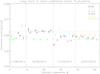 |
Fig. 1 C-band Jansky-to-counts conversion factor as measured for different calibrators in four observing sessions (separated by dashed vertical lines), spread over a 10-month timescale. Different colors correspond to different calibrators, as labeled in the panel. The dashed horizontal lines indicate the ± 0.002 rms variations around the average value of 0.06. For each observing session we report the date of the observations. |
For mapping experiments such as those reported in Sect. 7, it is important to verify whether the pointing accuracy is affected by the scanning speed. The tracking and scanning accuracy of the telescope was verified through OTF scans. Acquisitions consisted in Az/El cross-scans performed at different scanning speeds, at various elevation positions. Users of the SRT are requested to indicate a “sky speed” (i.e., the actual scanning speed measured “on sky”) in the observing schedules. For elevation subscans, such speed corresponds to the speed around the elevation axis. When scanning along azimuth, on the other hand, the sky speed translates into azimuth “axis speed” according to  (1)When performing each subscan, the antenna tracks the source in both azimuth and elevation, while running along a predefined path on the “scanning axis”. Incremental offsets are applied to the scanning axis motion, varying with a constant step within the defined span with respect to the instantaneous source position. Our data can thus indicate both the tracking (i.e., along the non-scanning axis) and the scanning accuracies.
This test was performed at K band only, i.e., where the pointing accuracy tolerance (≲5 arcsec) is the most stringent. In particular, we chose to observe in the 24.00–24.68 GHz sub-band, where the SRT beam size (HPBW = 46′′) is smaller and both the RFI and opacity contributions are less prominent with respect to lower frequencies within the K-band receiver RF range.
The pointing accuracy along the tracking axis turned out to be stable at the sub-arcsec level for any scanning speed. The positional offsets along the scanning axis is in line with the measured pointing offsets listed in Table 3, and proved to remain tolerable for “axis speeds” up to 20°/min. Deviations from this level of performance, showing pointing offsets up to 15′′, have been detected in a limited number of sessions (mainly for the elevation scans), regardless of the scanning speed. This phenomenon is likely related to thermal deformations of the telescope structure, indicating that the implementation of metrology-based corrections might be required, in the case of significant thermal variations, even when operating at K band.
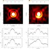 |
Fig. 2 SRT beam patterns at C-band (7.24 GHz, left-column panels) and K-band (right-column panels) respectively. For K-band we show only the 25.54 GHz measurement of the central beam. Top: elevation-averaged beam patterns (normalized to a peak value of 1) obtained by stacking together several OTF scans of bright point sources taken at different elevations. The color map has been intentionally saturated to highlight the low intensity features of the second and third lobes. Bottom: beam cross-sections along the azimuth and elevation axes (in dB). |
5.2. Detailed characterization of the beam pattern
The SRT beam shape was characterized as part of the technical commissioning activities (see Bolli et al. 2015), where residual deformations of the main lobe were measured as a function of elevation once the SRT optical alignment was optimized and the active surface was implemented. Here we provide a finer characterization of the SRT beam shape, and its possible variations as a function of telescope elevation, by extending the analysis from the main lobe only to the third lobe (or second side lobe). This finer beam characterization is particularly important for high dynamic range imaging in the presence of bright sources (see Sect. 7.1 for a demonstration). In this case, beam deconvolution is required, as the lateral lobes of the beam, if poorly known, can limit the final sensitivity of the image.
In this section, we report on the results obtained at C band and at K band, where a full characterization of each of the seven beams was obtained. The beam shapes at C and K bands were measured through a campaign of OTF scans in all possible coordinate frames (equatorial, horizontal, and Galactic), collecting a large number of maps along orthogonal axes: RA and Dec, Azimuth and Elevation, Galactic longitude (GLON) and latitude (GLAT). We sampled along rotated frames to reduce the artifacts related to the odd OTF sampling. The data were acquired using the TP backend. At K band, we observed at four different frequencies, distributed in the 8 GHz frequency range covered by the K-band receiver (18–26 GHz). The seven beams of the K-band feed array were characterized simultaneously.
Table 4 reports the observational details of the C- and K-band campaigns. For each target, we list the central frequency of the observations (νobs); the field of view (FoV), i.e., the region around the target that was imaged; the mapping speed (vscan); and the number of scans performed (half for left and half for right polarizations). The sampling interval and integration time were always set to 10 ms. The instantaneous bandwidth was always set to 680 MHz.
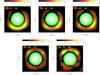 |
Fig. 3 Variation of the SRT beam pattern at 7.24 GHz as a function of elevation. Each image shows a field of view of 6′ × 6′ centered on the beam pattern peak (normalized to 1). Contour levels start at −25 dB and increase by 1 dB. |
For data calibration and analysis, we used the SCUBE data reduction software (Murgia et al. 2016, see Sect. 3.3 for a brief description). The beam pattern was obtained through iterative wavelet modeling. An increasingly refined baseline subtraction and a “self-calibration” were applied to remove the residual elevation gain variations and pointing offsets from the individual OTF scans.
The self-calibrated OTF scans were combined to derive a detailed model of the SRT beam pattern at C and K bands down to the third lobe (see Fig. 2 left column and right column panels, respectively). The elevation-averaged beam patterns (in Jy/beam) are shown in the top panels. It is evident that we successfully detected the third lobe of the SRT beam pattern. The bottom panels show two perpendicular beam cuts intercepting the peak. One is directed along the azimuth axis (upper panel) and the other along the elevation axis (lower panel).
Observational details of the SRT beam characterization campaigns at C and K bands using the TP backend.
The expected size of the beam pattern main lobe at 7.24 GHz is HPBW = 2.6 arcmin. The inner 4′ × 4′ of the main lobe of the beam pattern at this frequency was measured by fitting the target source with a 2D elliptical Gaussian with four free parameters: peak, minimum and maximum full-width half-maximum sizes (FWHMmin and FWHMmax), and position angle (PA). We found FWHMmin = 157′′ and FWHMmax = 158′′, with PA ≃ 0°, confirming that the SRT main lobe at 7.24 GHz can be considered to be circularly symmetric with FWHM = 2.62′. The secondary lobe intensity averaged over an annulus of 4.5′ radius and 3′ width is –24 dB. The secondary lobe is clearly asymmetric, being brighter below the main lobe. We anticipate that this asymmetry is elevation dependent, as further discussed below. The average intensity of the third lobe over an annulus of 9′ in radius and 3′ in width is –33 dB. The most striking features associated with the third lobe are the four spikes seen at the tips of a cross tilted by 45°. These originate from the blockage caused by X-shaped struts sustaining the secondary mirror in the path of radiation between the source and the primary mirror.
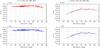 |
Fig. 4 Gain (in K/Jy) as a function of elevation measured through OTF scans at 7.24 GHz (left panels) and at 25.54 GHz (right panels), with a bandwidth of 680 MHz. The right and left polarizations are shown separately (top and bottom panels respectively). The solid lines represent fourth order polynomial fits. The 25.54 GHz gain curve refers to the central feed of the K-band receiver. |
To study the variation of the beam shape with elevation, we grouped the OTF scans at C band into five bins of 15° in width. A zoom of the inner 6′ × 6′ showing variations of the second lobe asymmetry with a slightly finer elevation binning is presented in Fig. 3. It is clear that the beam pattern varies significantly with elevation. The most important effect is the behavior of the secondary lobe structure. In particular, we observe a flip of the asymmetry around an elevation of 60°. At elevations higher than 60°, the brightest part of the secondary lobe is observed above the main lobe, while it is observed below it at mid and low elevations. The same behavior is observed for the K-band beam (not shown).
The expected size (HPBW) of the main lobe of the beam pattern at K band varies from ~ 1 arcmin (at 18 GHz) to ~ 0.7 arcmin (at 26 GHz). Here we report on the results obtained at 25.54 GHz for the central feed (shown in Fig. 2, right panels). The results obtained for the other three frequencies and for the other feeds are qualitatively similar. By fitting the target source with a 2D elliptical Gaussian with four free parameters, as done at C band, we found FWHMmin = 43′′ and FWHMmax = 48′′, with PA ≃ 0°. This clearly indicates that the main lobe of the SRT at K band is no longer circularly symmetric, but rather slightly elliptical. The asymmetry of the secondary lobe is even more pronounced with a very bright peak below the main lobe (–12 dB, see elevation cut). This asymmetry does not satisfy the SRT design specifications (secondary lobe below –20 dB).
The current LUT was built through photogrammetry measurements in six elevation positions. Our tests seem to suggest that denser elevation-dependent measurements are needed to correct the residual misalignments of the telescope optics, which affect the K-band beam pattern. In addition, the LUT of the secondary mirror was built during the first SRT optical alignment (see Bolli et al. 2015) and was mainly aimed at correcting the much larger primary mirror deformations. A laser tracker measurement campaign is currently ongoing to map the position of the secondary mirror as the telescope varies in its elevation angular range with and without using the LUT. Thanks to the sub-millimetre accuracy of the laser tracker16, we can finely measure the translations and the rotations of the secondary mirror at several elevation angles of the telescope, and refine the LUT mainly at low (but even at high) elevation angles where some residual misalignments are still present.
We point out, however, that even in the present situation, the SRT offers excellent imaging capabilities, in particular when combined with deconvolution techniques. This is illustrated in Sect. 7.
5.3. Fine characterization of the gain curve
An important by-product of the in-depth characterization of the primary beam at C and K bands (see Sect. 5.2) is a very reliable measurement of the gain curves at fine steps in elevation. Indeed, the best-fit peak amplitude obtained through self-calibration, divided by the target flux density, directly yields the antenna gain in K/Jy. In Fig. 4 we present the gain curves measured at 7.24 GHz (left panels) and at 25.54 GHz (right panels) separately for the right (top) and left (bottom) polarizations.
At C band, the gain curves were derived using the observations of the calibrator 3C 147 (see Sect. 5.2) and assuming a flux density of 5.43 Jy at 7.24 GHz for the target (Baars et al. 1977 scale). The measured median gains are 0.63 and 0.62 K/Jy for right and left polarizations, respectively, with a scatter of about 8–9%. These values are slightly higher than those measured during the SRT technical commissioning activities (see Bolli et al. 2015 and our Table 2) and are closer to the expected values (see Table 2.2 of Bolli et al. 2015). The gain curves are extremely flat, indicating that the active surface is performing very well.
The gain curves measured at 25.54 GHz for the central feed of the K-band receiver were obtained from the observations of the bright radio source 3C 84 (see Sect. 5.2). We corrected the OTF scans for the atmosphere opacity and we used the primary calibrator 3C 295 to derive the 3C 84 flux density (26.83 Jy at 25.54 GHz; Perley & Butler 2013 scale). Figure 4 (right panels) clearly shows a decrease in efficiency below 45° of elevation, while the gain curve is flat at higher elevations. This confirms what was found during the commissioning activities (Bolli et al. 2015) and indicates that the modeling of the gravity deformations at low elevations can be improved (see Sect. 5.2). However, we measure a maximum gain of ~ 0.58 K/Jy for both polarizations. This value is lower than that measured during the commissioning at a frequency of 22.35 GHz (see Bolli et al. 2015 and our Table 2). However it is still in line with the expectations for the K-band receiver (0.6–0.65 K/Jy, see Table 2.2 of Bolli et al. 2015).
As discussed in Sect. 5.2, the gain curves presented here are obtained through OTF imaging. These curves are fully consistent with others obtained through standard procedures based on cross-scans. This novel technique based on imaging is particularly efficient for multi-feed receivers, since it allows us to obtain the gain curves for all beams simultaneously. The measurements obtained for the lateral feeds of the K-band receiver are very similar to those for the central feed and are not shown.
The SRT gain curves are regularly updated on the SRT website.
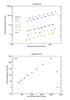 |
Fig. 5 Source (baseline-subtracted) amplitude vs. peak (source + baseline) level, both expressed in raw counts. Increasing raw counts on both axes reflect decreasing attenuation. Top panel: illustration of the test performed with 250 MHz bandwidth at a central observing frequency of 7.25 GHz. Different sources are indicated by different colors, as labeled in the panel. Bottom panel: illustration of the test performed with 1200 MHz bandwidth at a central observing frequency of 6.8 GHz. Here only the bright source 3C 286 (5.87 Jy at 6.8 GHz, Perley & Butler 2013) is shown, to highlight the levels of raw counts where saturation is reached. |
6. Radio-continuum observations with the total power backend
In the following, we report the on-sky characterization of the TP backend. The tests discussed here provide a useful reference for future telescope users. In addition, a good characterization of the TP is a prerequisite for efficiently conducting high-performance imaging experiments, such as those discussed in Sect. 7.
6.1. Backend linearity
The response of the TP backend was tested through the execution of cross-scan observations of a selection of well-known sources from the B3-VLA catalog (Vigotti et al. 1999) with the addition of a number of other widely used calibrators. This test, which is band independent, was carried out at C band. The selected sources range in flux density from a few tens of mJy to a few Jy (flux densities measured at 4.85 GHz). The observations were performed for varying bandwidths and attenuation settings to span a wide range of “raw counts” signal levels and probe the backend linearity range. The results are summarized in Fig. 5. The top panel of Fig. 5 shows the results obtained for different sources by setting a bandwidth of 250 MHz. It is clear that the backend response is linear over a wide range of raw counts, from ~ 200 to ~ 2000 counts (x-axis). With a narrow band of 250 MHz, saturation is never reached even with no attenuation (=0 dB). For sources with flux density <100 mJy, saturation cannot be reached, regardless of the bandwidth or the attenuation setting. The bottom panel of Fig. 5 shows the result for the bright source 3C 286 only (5.87 Jy at 6.8 GHz, Perley & Butler 2013), when setting a larger bandwidth of 1200 MHz. This plot clearly shows that saturation is reached around 2000 raw counts. Since the backend linearity is well preserved at low baseline levels, it is recommended to work at levels of a few hundred counts (e.g., ~400–500 counts), so as to fully exploit the available dynamic range.
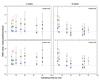 |
Fig. 6 Ratio of measured over expected noise as a function of sampling interval for different bandwidths (blue circles = 250 MHz, green squares = 680 MHz, and red diamonds = 1200 MHz). The noise RMS is measured (and estimated) over different time windows. Here we show the results for 2 s (top) and 4 s (bottom) time windows. The experiment was performed at both C (left panels) and K band (right panels). |
6.2. Band-limited noise and confusion limit
This experiment focused on the measurement of the radio continuum noise, which was recorded by selecting different bandwidths and sampling intervals. Ideally, as long as the post-detection integration time is short enough that 1 /f noise effects are not dominant, the measured noise is supposed to be band limited; i.e., this noise should coincide with a white noise whose RMS value (σ), given a certain system temperature, depends only on the selected bandwidth and on the integration time, according to the radiometer equation 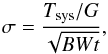 (2)where the antenna gain is given in K/Jy, the system temperature in kelvin, the bandwidth in hertz, and the integration time, t, in seconds. The aim of this test was to verify whether – and for which bandwidths – the thermal noise, estimated through the radiometer equation, could be reached. This test is particularly relevant for the TP, as analog backends do not allow an efficient removal of RFI-affected data, and this can easily result in increased noise levels, especially when large bandwidths are used.
The experiment was performed at both C and K bands. The observing frequencies were chosen to minimize the presence of RFI (see Bolli et al. 2015). At C band, we set the low end of the bandwidth at 7 GHz. At K band, we set the low end of the bandwidth at 24 GHz. We acquired data employing different setups; we varied the bandwidth from 250 to 1200 MHz, while data sampling ranged from 10 to 80 ms. The subsequent noise RMS measurements were performed over different time windows to reveal possible effects and instabilities at different timescales. Figure 6 shows the results for C band (left panels) and K band (right panels), in terms of the measured observed-to-expected RMS ratio, for either 2 s (top) or 4 s (bottom) time windows. All plots clearly show a band-related increase of the noise ratio, where the measured noise is very close to expected for the smallest bandwidth (250 MHz), and becomes a factor of 1.5–2 larger when increasing the bandwidth to 1200 MHz. This is probably due to low-level RFI, whose impact on continuum observations becomes larger for wider bandwidths, as more polluting signals are likely to be gathered in a wider frequency range. This increase is more pronounced at C band, since it is more severely affected by RFI. The noise ratio also increases with the time window. This is probably due to instabilities and gain drifts becoming visible in the 4 s time frame, leading to a measured signal that is not purely white noise anymore. These measurements allowed us to confirm that band-limited noise can be reached by the TP, at least for narrow bandwidths. Moreover, the effects due to RFI can be kept under control by properly setting the observing frequency.
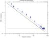 |
Fig. 7 Measured RMS noise as a function of integration time. The oblique solid line shows the expected trend according to the radiometer equation. The parallel dot-dashed line corresponds to the theoretical noise increased by 25%. The horizontal dot-dashed line shows the measured confusion limit. |
Another important parameter that must be estimated – when planning observations – is the integration time needed to reach the desired sensitivity. A dedicated test was carried out to verify whether the noise decreased with integration time (t) following the expected  law described by the radiometer equation (see Eq. (2)). The experiment was performed at C band, where the system temperature is very stable over a wide range of elevation positions (20–80°) and the gain curve is almost flat (see Bolli et al. 2015). This means that variations of the telescope performance parameters with elevation did not affect our measurements. The observations were carried out at a central observing frequency of 7.5 GHz with a bandwidth of 250 MHz. They consisted of repeated back-forth OTF scans along RA, acquired over a selected “empty sky” strip. This was chosen within a deeply mapped area of the 10C survey (AMI Consortium: Davies et al. 2011); more specifically, the strip was centered on RA = 00h27m00ss, Dec = +31°35′00′′ and it covered an RA span of 0.5°. No sources with a flux density greater than 0.1 mJy at 10 GHz are known to exist in this strip. The scans were inspected, flagged, and iteratively summed to measure the RMS noise for increasing integration times. The results are shown in Fig. 7. Raw data were calibrated employing the front-end noise diode. Antenna temperature values were then converted into flux density by applying the gain curve. We find that the RMS noise decreases with integration time as predicted by the radiometer equation, all the way down to the so-called confusion limit, i.e., the impassable noise plateau produced by the presence of background faint unresolved sources falling in the telescope main beam. However, the RMS noise that is actually measured is ~ 25% higher than the theoretical value; this discrepancy can be ascribed to the overall instabilities arising from long exposure times (as described above). The higher noise level, of course, implies that the confusion limit is reached in a longer-than-predicted exposure time, amounting to ~ 430 s/beam.
The SRT ETC (see Sect. 3.1) provides an estimate of the confusion noise at the center of the observing band. This estimate is based on extrapolations of known source counts to different frequencies and/or lower flux densities (for details see Zanichelli et al. 2015). Using the algorithm implemented in the ETC, we get ~ 0.19 mJy at 7.5 GHz, our observing frequency. The actual measured confusion noise is 0.17 ± 0.02 mJy/beam, so this noise level is consistent with the predicted value. We can therefore conclude that the ETC provides a reliable indication of the telescope confusion limit.
7. Imaging capabilities of the SRT
In this section, we seek to demonstrate the radio-continuum imaging capabilities of the SRT. Such capabilities can be inferred through the assessment of the so-called dynamic range and image fidelity. The dynamic range (defined as the peak-to-noise rms ratio) identifies the ability to reach the thermal noise and/or to image faint or low-surface brightness in the presence of very strong sources. The image fidelity is a measure of the reliability of the image (in terms of surface brightness, size, and morphology) when mapping extended sources. In the following, we discuss the SRT capabilities for both the aforementioned parameters, focusing on radio continuum observations with the TP backend at C and K bands. As mentioned in Sect. 2, the use of analog backends, such as the TP, at L and P bands, is not recommended owing to severe RFI pollution.
The results illustrated in this section demonstrate not only the imaging capabilities of the SRT and of its receiving/acquisition systems, but also the role that can be played by innovative ad hoc imaging techniques, based on OTF scans and state-of-the-art data analysis software (e.g., SCUBE and SDI, which are described in Sect. 3.3).
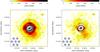 |
Fig. 8 Left panel: “Dirty” image of Virgo A resulting from the combination of 10 OTF scans achieved with the multi-feed K-band array at a frequency of 19 GHz and a bandwidth of 2 GHz. Close to the source the dynamic range is limited to ~ 30, due to the strong secondary lobes. Right panel: CLEANed image restored with a circular Gaussian with FWHM of 57′′. The measured surface brightness RMS sensitivity is now 1.3 mJy/beam and the dynamic range increases to 11 300. In both panels, contours start from 3σ and increase by a factor of |

7.1. Dynamic range and deconvolution techniques
Image fidelity and dynamic range are usually primarily limited by secondary lobes of the antenna radiation pattern rather than by thermal noise fluctuations. In this section, we aim to demonstrate the imaging capabilities of the SRT, in combination with deconvolution techniques, in the presence of a very bright point source that can severely limit the dynamic range. For this purpose, we chose to image Virgo A, which is one of the most challenging sources in this respect, and we exploited the SCUBE software package, which was optimized for SRT data reduction and analysis and includes deconvolution capabilities (see Sect. 3.3 for more details).
Virgo A is the fourth brightest radio source in the northern sky and is associated with M87, which is the galaxy at the center of the nearest rich galaxy cluster (Virgo). The AGN hosted by this elliptical galaxy is powered by one of the most massive active black holes discovered so far (MBH ≃ 6.4 ± 0.5 × 10⁹M⊙; Gebhardt & Thomas 2009). For these reasons, it has been the subject of a large number of studies at all wavelengths, from the radio to the X-ray. In the radio band, this source has been studied at low frequencies with interferometers such as the Very Long Array (VLA) and the LOw-Frequency ARray (LOFAR). These observations (Owen et al. 2000; de Gasperin et al. 2012) reveal similar morphologies: the radio source is composed of a bright inner double, which contains a collimated one-sided relativistic jet pointing toward the northwest that is embedded in a low surface brightness halo of synchrotron plasma. The angular size of the inner double is about 1 arcminute, corresponding to about 5 kpc in linear size. The faint halo extends for 15 arcmin (or 80 kpc). Despite its comparatively lower surface brightness, the extended halo is responsible for much of the flux density. Owing to the large difference in surface brightness between the halo and the inner double, high-dynamic range imaging of Virgo A has always represented a big challenge. At high radio frequencies (ν > 1 GHz), interferometric observations are nearly impossible because of the large angular size of the source. On the other hand, large single dish antennas with low-noise receivers and large collecting areas, such as the SRT, provide enhanced surface brightness sensitivity for the detection of faint large-scale radio emission and the recovery of the flux density missed by interferometers. Multiwavelength observations and spectral studies (see de Gasperin et al. 2012) can indeed provide important information about the relationship between the compact inner double and the extended halo in Virgo A, which is still matter of debate.
We observed Virgo A at K band through multi-feed OTF scans, on November 15, 2015. Data were acquired with the TP backend at a central frequency of 19 GHz and a bandwidth of 2 GHz. We mapped a FoV of about 0.5° × 0.5° with 121 subscans spaced by 15 arcsec on the sky using the derotator fixed in angle in the equatorial frame. We interleave the OTF scans with a telescope sky dip every hour to determine the trend of the optical depth τ during the observation and to correct the data to compensate for the atmosphere opacity (τ ≃ 0.05 during these observations). The scanning speed was set to 6 arcmin s-1, and we sampled at 10 ms. We acquired 10 OTF scans, 5 along the RA direction plus 5 along the Dec direction. We obtained useful data from 12 outputs of the multi-feed (7 from the left-circular polarization channel and 5 from the right-circular polarization channel), thus we collected a total number of 120 images centered on Virgo A. Multi-feed data reduction was performed with the SCUBE software package. We observed 2 OTF mapping of the primary calibrator 3C 286 that we used to convert the raw counts to the flux density scale of Perley & Butler (2013) for all the seven feeds of the K-band array. We also corrected for variation of telescope gain with elevation using the curves derived during the AV (see Sect. 5.3).
Figure 8 (left panel) shows the image obtained for Virgo A. As explained in Sect. 5.2, the asymmetries of the secondary lobes of the K-band beam patterns are strong and limit the dynamic range to ~ 30 close to the source. Standard deconvolution techniques, such as those implemented for radio interferometry data, can help to remove the beam side lobes and effectively reach the thermal surface brightness RMS sensitivity (expected to be ~ 1 mJy/beam for a pixel size of 15 arcsec, by applying Eq. (2)). In particular, it is necessary to perform a precise characterization of the telescope beam pattern followed by its accurate deconvolution from the dirty image of the sky brightness. Owing to elevation-dependent asymmetries (see Sect. 5.2), we need to employ an elevation-dependent beam model for a proper deconvolution of the sky image from the antenna pattern.
We used the wavelet beam model obtained on 3C 84 (see discussion on Sect. 5.2) to deconvolve the antenna multi-feed beam pattern from the “dirty” image of Virgo A in the Equatorial frame using the SCUBE software. The CLEAN algorithm rotates and interpolates the beam pattern model by taking into account the specific elevation and parallactic angle for each individual data point. For Virgo A, we measure a peak surface brightness of about 14.7 Jy/beam on the cleaned imaged. We convolved the CLEAN components with a circular Gaussian with FWHM 57′′ (shown in the bottom right corner of the right panel) and restored with the residual image. The resulting image is shown in the right panel of Fig. 8. The side lobes are not an issue anymore, the noise is 1.3 mJy/beam (very close to the expected thermal noise) and the dynamic range increases to 11 300. The improvement obtained with the deconvolution is indeed very significant and allows us to reveal the faint and diffuse outer lobes of the radio source that were hidden below the secondary lobes of the beam pattern.
Figure 8 (right panel) represents the highest frequency observation ever achieved for Virgo A at arcminute resolution, superseeding the image of the halo of Virgo A obtained at 10.55 GHz with the Effelsberg radio telescope at 69 arcsec resolution (Rottmann et al. 1996). At the SRT resolution, the inner double cannot be resolved, but our high-dynamic range observation has enough sensitivity to detect the full extent of the halo.
The K-band multi-feed high-dynamic range imaging of Virgo A is perhaps the most complex imaging test performed during the AV, pushing the SRT to the limits of its present capabilities as a single-dish imaging instrument. This system is also targeted as part of one of the early science SRT projects. For a full analysis of the high-frequency spectral properties of Virgo A, we therefore refer to a future paper (Murgia et al., in prep.) where the results of this project will be reported.
7.2. Dynamic range: extended sources
In the previous section, we dealt with the case of an extremely bright point source, which required the implementation of deconvolution techniques to achieve good image quality. Here we want to determine the SRT dynamic range capabilities to map very large-scale, low-surface-brightness emission, filling up most of the field of view, with bright point sources embedded in it. In this case, deconvolution techniques are not essential, as the side lobes produced by the bright point sources affect only a very limited portion of the image. For this purpose, we imaged two well-known Galactic extended sources: the Omega Nebula and the W3 molecular cloud complex.
The Omega Nebula and the W3 molecular cloud complex are considered to be among the brightest and most massive star-forming regions of our galaxy and are known to be very interesting examples of maser and radio recombination line sources (se OH and methanol maser measurements presented in Sect. 8). The continuum radio emission from these objects is mostly due to free-free radiation emitted by hydrogen ionized from the ultraviolet photons produced by young and massive stars. Both the Omega Nebula and W3 star-forming regions have been imaged as part of the commissioning of the GBT. This means that we can directly compare the imaging capabilities of two state-of-the-art instruments at similar observing frequencies and resolution.
We observed the two targets in the period October–November 2014. We performed OTF maps along RA, Dec, GLON, GLAT, Azimuth, and Elevation directions. The data were acquired using the TP backend at a central observing frequency of 7.24 GHz and with a bandwidth of 680 MHz. The main observational parameters of both sources are listed in Table 5. For each target we list the imaged FoV, mapping speed vscan, integration time tint (equal to the sampling time) and total time ttot spent on each target. The results are discussed below.
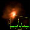 |
Fig. 9 Continuum image of the Omega Nebula obtained with the SRT at 7.24 GHz. The source emission shown extends over about a 1o × 1o region. The RMS noise is ≃7 mJy/beam and the SRT resolution is 2.6 arcmin (SRT beam size at 7.24 GHz). The color map was biased to highlight the low surface brightness emission. As a result, the central and brightest part of the nebula (M17-UC1), characterized by a surface brightness in the range ≃3–100 Jy/beam, is saturated. Inset spectrum:6035 MHz OH maser emission (Jy) observed toward M17-UC1 is shown. Left and right circular polarizations are indicated in yellow and green, respectively. The spectrum was acquired with XARCOS, pointing at the position (J2000) RA = |

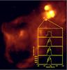 |
Fig. 10 Continuum image of W3 obtained at 7.24 GHz with the SRT. The field of view is about 2o × 2o. The RMS noise is ≃4 mJy/beam and the resolution is 2.6 arcmin (SRT beam size at 7.24 GHz). The color map has been saturated to highlight the low surface brightness emission. Inset spectrum: 6.7 GHz methanol maser emission (Jy) in W3OH is shown. The spectra were taken with XARCOS on January 28, 2016. Four sub-bands (see panels) were observed simultaneously at increasing spectral resolution. Specifically we show spectra with 1.4 km s-1, 170, 40, and 10 m s-1 channel widths (from top to bottom). Left and right circular polarizations have been averaged. The velocity scale refers to the LSR frame and uses the optical convention (for more details see Sect. 8). |
As for Virgo A (see Sect. 7.1), the data of the Omega Nebula and the W3 molecular complex were reduced and analyzed using the SCUBE software. In this case, though, deconvolution techniques were not applied. We note that to evaluate the robustness of our surface brightness measurements, we also imaged two well-known calibrators, 3C 295 and 3C 147, with an OTF mapping setup similar to that of the targets. These calibrators were analyzed through the same strategy adopted for the Omega Nebula and W3, and the measured flux densities (on the Baars et al. 1977 scale) were checked for consistency against values from the literature.
The image obtained for the Omega Nebula after flagging of RFI-corrupted scans, data calibration, baseline subtraction, imaging, and combination of the six OTF maps obtained, is shown in Fig. 9. The nebula peaks at a surface brightness of 101.5 Jy/beam, and presents a northwest – southeast orientation with a sharp edge on the west side. Two patches of extended emission are visible in the bottom right corner of the image. This is also the direction of the Galactic plane. The radio emission fades from the center of the nebula outward, but it is clear that the faint extended emission covers the entire field of view of our observation. This limits the possibility of calculating the noise with a good precision. We evaluated a noise of ≃7 mJy/beam. The resulting image dynamic range, measured as the peak to noise ratio, is ~ 14 500.
Figure 10 shows the image obtained for a field of view of about 2o × 2o, which includes the W3 main molecular cloud (the brightest structure visible on the top right, which hosts the ultra-compact HII region W3) and the low surface brightness emission extending toward the southeast, which is catalogued as IC 1805 (also known as the Heart Nebula). We evaluated a noise of ≃4 mJy/beam. Considering that the peak of the emission associated with W3 Main reaches a surface brightness of 35.8 Jy/beam, the resulting dynamic range is ≃9000. In addition to the thermal emission associated with the W3 and IC 1805 star-forming region, we also observed a handful of point sources that are likely background extragalactic objects.
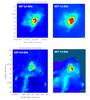 |
Fig. 11 Comparison of GBT (left panels) and SRT (right panels) images of the Omega Nebula (top) and W3(OH) (bottom). The GBT commissioning observations of the Omega Nebula and of W3 were obtained at 8.4 GHz (Prestage & Maddalena 2003) and 8.9 GHz (GBT site), respectively. |
For a qualitative assessment of the imaging capabilities of the SRT in comparison with the GBT, we show in Fig. 11 the commissioning GBT images of the Omega Nebula (top left panel) and W3 (bottom left panel) obtained at 8.4 GHz and 8.9 GHz, respectively, along with the SRT images at 7.2 GHz (top right and bottom right panels). For a better comparison, the SRT images were rendered using a similar color map, saturation, and field of view to the GBT images. The GBT images have an angular resolution that is better by a factor of two. As a consequence, the bright compact features appear better detailed in the GBT images. However, the SRT images recover all of the structures seen by the GBT and, in addition, the smoother resolution provides a better signal-to-noise ratio (S/N) for the faint and extended radio emission associated with the nebula. Indeed, we found that SRT could reach dynamic range levels comparable to those reached with the GBT (i.e., ~ 10 000), at least in the case of Omega Nebula. It is important to stress that the high dynamic range levels quoted above for extended sources were obtained without deconvolution of the SRT beam pattern, In fact, the secondary lobes of the beam affect only the regions very close to the peak of the emission in these images. In these cases, the very accurate baseline subtraction allowed by the SCUBE software have proved to do an excellent job.
7.3. Image fidelity: galactic plane sources
The image fidelity capabilities of the SRT were tested through observations of well-known SNRs. Among them, IC443 represents an ideal target in this respect, owing to its interesting complex morphology, the availability of extensive multiwavelength data, and its good visibility at the SRT site.
IC443 (also named 3C 157), located at about 1.5 kpc in the direction of the Galactic anticenter (Heiles 1984; Braun & Strom 1986), is one of the best-studied Galactic SNRs. The large structure of the source extends over 0.75o and shows evidence of interactions with both atomic and molecular clouds (Snell et al. 2005). The discovery of a neutron star in X-rays with Chandra (Olbert et al. 2001) suggests a core-collapse origin for the SNR. Its integrated flux density at 1 GHz is about 160 Jy (for a detailed discussion of this source, see Green 2014 and references therein).
We observed IC443 in the period May–December 2014. We performed OTF maps along RA and Dec directions. The data were acquired using the TP backend at a central observing frequency of 7.24 GHz and with a bandwidth of 680 MHz. The main observational parameters of the source are listed in Table 5. The adopted observing parameters typically imply the acquisition of >10–20 samples/beam for each subscan passage (largely oversampling the beam w.r.t. Nyquist sampling). This allows us to get an accurate evaluation of flux density errors and efficiently reject outlier measurements ascribed to RFI. The offset between two consecutive subscans was set to 0.01o, which implies on average 4.5 passages per beam and about 17 samples per beam per scan (assuming a beam size of 2.7′′ at our observing frequency). The total duration of an observation (single map RA+Dec) was about 3 h including dead and slew time.
The length of the subscans (or the image size) was chosen according to the size of the source. The subscan-dependent baseline (background) must be correctly subtracted to properly reconstruct the morphology of the observed source and its associated flux density. Ideally, each subscan should be free from significant source contribution (and RFI contamination) for 40–60% of its length or duration to properly identify and subtract the baseline component. This requirement is not trivially achieved for targets located in crowded regions of the Galactic plane. The flux density calibration was based on cross-scan observations of six bright point sources: 3C 147, 3C 48, 3C 123, NGC 7027, 3C 295, and 3C 286.
For data reduction and analysis, we used the SDI software, developed as part of the AV activities with the purpose to make it available to SRT users. The SDI software provides a pipeline for data inspection, RFI rejection, baseline removal, and standard image calibration, optimized for the SRT (see Sect. 3.3 for more details). While not allowing deconvolution (allowed by SCUBE), SDI provides innovative and accurate baseline subtraction techniques required for the imaging of crowded regions close to the Galactic plane (see Pellizzoni et al., in prep., for more details). An additional aim of this test was therefore to assess the SDI performance and its robustness in its automated operation mode. A calibrated SDI image obtained for SNR IC443 is shown in Fig. 12 where it is compared with VLA+Arecibo observations. The SRT image offers a detailed view of the supernova remnant morphology, which is remarkably similar to that obtained through VLA interferometric observations carried out at lower frequency (1.4 GHz) and at a factor 2–4 higher resolution. We estimated an image rms of ~ 10 mJy/beam and a dynamic range of ~125; RFI typically affected <10% of samples in the adopted band and were automatically flagged by SDI.
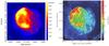 |
Fig. 12 Images of SNR IC443. Left: single-dish 7.24 GHz calibrated image obtained with the SRT (2.7′ resolution; image RMS ~ 10 mJy/beam for an effective exposure time of 6.5 h). Right: 1.4 GHz continuum 7-pointing mosaic obtained with the VLA (40′′ resolution) in combination with Arecibo (3.9′ resolution) data to provide sensitivity to extended low surface brightness emission (total observing time 6.3 h). The blue arrows indicate the position of two extra-galactic background sources, and the black arrow indicates the neutron star (from Lee et al. 2008). |
The integrated flux density measured for IC443 is 64 ± 3 Jy. This is consistent at a 1σ level with the expected value of 73 ± 10 Jy, derived from the value of 84.6 ± 9.4 Jy measured at 4.8 GHz with Urumqi (the Sino-German 25 m telescope used to carry out a polarization survey of the Galactic plane), when assuming an overall spectral index of −0.38 ± 0.1 (Gao et al. 2011). The main uncertainties in this flux comparison are the different angular resolutions of the two measurements (2.7′ SRT and 9.5′ Urumqi) and the uncertainty on the source size over which Gao et al. (2011) integrated the flux.
For further details on C-band observations of SNRs with SRT and related early science outcomes, we refer to Egron et al. (2016, 2017b).
8. Spectroscopy with XARCOS
At the end of 2015, the XARCOS multi-feed digital correlator was fully integrated into the SRT control system Nuraghe (Melis et al. 2015). A number of observations were then performed at the SRT to demonstrate its capabilities. In particular, we performed observations of maser lines in a handful of well-known Galactic star-forming regions. In the following, we report on spectral line (maser) observations taken at C band on two targets: the Omega Nebula and W3(OH).
Observations of both targets were performed on January 28, 2016, using the standard position-switching mode. We used the mono-feed C-band receiver, which provides dual circular polarization. On-source and off-source scan integration times were equally set to 60 s. The off-position was shifted in declination by two degrees from the target coordinates to account for the large extension of the nebula. The spectropolarimeter XARCOS was configured in the standard “XC00” mode, which provides four bands of 62.5, 7.8, 2.0, and 0.5 MHz, with 2048 channels for each band. This setup resulted in channel spacings of 1.5, 0.2, 0.05, and 0.01 km s-1 for the four bands, respectively.
The Doppler correction for tracking the maser lines was performed by the FTrack software (Orlati et al., in prep.), which was fully implemented in the antenna control system by the time of our observations. The data reduction was performed with the Gildas software, after the SRT FITS data were converted into Gildas format using the “Srt_class_writer” package (Trois et al., in prep.).
8.1. Omega Nebula
We observed the OH  , J = 5/2, F = 3 → 3 hyperfine transition, (rest frequency 6035.085 MHz17) toward the ultra-compact HII region M17-UC1 in the Omega Nebula. Each section was centered on the frequency corresponding to the VLSR velocity of the strongest maser feature (21.0 km s-1) reported in Knowles et al. (1976). We used the calibration mark and gain curve presented in Sect. 5.3 to establish the flux density scale of each polarization separately. We estimate that the accuracy of our absolute flux density scale is on the order of ~10%.
Excited-state OH maser emission at 6035 MHz was first discovered toward M17 by Rickard et al. (1975) and confirmed by Knowles et al. (1976), who detected strong emission features at VLSR = 21.0 km s-1 and VLSR = 22.1 km s-1. A third, more redshifted component was detected in later observations in the left polarization spectrum (Caswell & Vaile 1995; Fish et al. 2006). The line at VLSR = 21.0 km s-1 was found to be partially elliptically polarized (Knowles et al. 1976). In addition, a separation of ~0.04 km s-1 from the opposite circular polarization was measured for this line, which was attributed to Zeeman splitting in a +0.8 mG magnetic field (where the positive sign indicates that the component of the magnetic field along the line of sight is pointing away from us; Fish et al. 2006). We detected all three components in the left circular polarization spectrum of M17-UC1 and two in the right. The spectra are shown in the inset of Fig. 9. The results of Gaussian fitting to the line profiles are presented in Table 6, where for each component and each polarization we list the line velocity (VLSR), line width (FWHM), peak flux density (Speak), and flux density integrated over the line (∫SdV).
The line velocities are consistent with those measured by Knowles et al. (1976), assuming a 0.1 km s-1 uncertainty in their measurements. We detected a Zeeman splitting of the strongest feature of 0.048 ± 0.005 km s-1 that directly yields a magnetic field of +0.86 mG, using the formula reported in Baudry et al. (1997). Our result confirms the estimate made by Fish et al. (2006) with a higher accuracy and confidence due to the higher spectral resolution of the XARCOS spectra.
We caveat that Zeeman splitting determinations can be affected by systematics, such as beam squint, which consists of the two (right and left) circular polarizations pointing to two slightly different directions (Heiles 1996), and/or small amplitude non-Gaussian effects on the spectral baselines (Vlemmings 2008). Methods to calibrate these effects are discussed in, for example, Heiles et al. (2001) and Vlemmings (2008). In this work, as in Fish et al. (2006), we did not attempt to account for such systematics. Vlemmings (2008) estimated a contribution of beam squint to the measured magnetic field smaller than 40 μG in the case of W3(OH) 6.7 GHz methanol masers observations conducted with the Effelsberg radio telescope. We notice that W3(OH) represents a sort of worst-case scenario because it is one of the most extended maser emission sources, and beam squint effects are smaller when the maser region consists of individual compact features that dominate the spectrum, as for the case studied in this work.
Characterization of the SRT circular polarization performance for spectral – maser – line observations is currently ongoing, including the estimate of the beam squint discussed above. The characterization of the linear instrumental polarization, on the other hand, has already been successfully conducted and is presented in Murgia et al. (2016).
Line parameters of the excited-state OH maser toward the ultra-compact HII region M17-UC1 in the Omega Nebula.
Line parameters of the CH3OH maser in W3OH.
8.2. W3OH
We observed the (51–60) 6.7 GHz CH3OH maser transition (rest frequency 6668.52 MHz) toward the famous ultra-compact HII region W3(OH), known to also host strong maser emission from several other molecular species (e.g., water and hydroxyl). Each section was centered on the frequency corresponding to the VLSR velocity of the strongest maser feature (–45.1 km) reported in Menten (1991). As primary flux calibrator, we observed 3C 286. The flux calibration was performed by estimating the average value of counts of the continuum in the on-off/off spectrum of 3C 286 for the different sub-bands. This value (~ 0.14 for all subbands and both polarizations) was used in conjunction with the expected flux density value of 3C 286 at the observed frequency (6.11 Jy, computed following Baars et al. 1977) to convert counts into Jansky.
The main methanol maser line in W3OH is confidently detected in all four sub-bands. Figure 10 (inset spectrum) shows the XARCOS ability to provide simultaneous spectra at four different resolutions, from the lowest resolution (30.5 kHz or 1.4 km s-1 at 6.7 GHz) spectrum covering a relatively broad frequency bandwidth (62.5 MHz, top panel) to the highest resolution spectrum (240 Hz or 10 m s-1 at 6.7 GHz) over a narrow bandwidth (0.488 MHz, bottom panel). The former is particularly well suited to provide information on emission throughout the velocity field of the source, while the latter allows us to study line profiles in detail, revealing, for example, blue- or redshifted wings and/or complex line subcomponents. In particular, up to six features are revealed in the highest resolution spectra of the main methanol maser line in W3OH. A multi-Gaussian fit of the highest resolution W3(OH) spectrum was performed utilizing the XGAUSSFIT routine of the FUSE IDL Tools18. The results are presented in Table 7 (columns are as in Table 6; left and right polarizations were averaged in this case). The flux density of the peaks are consistent, within the uncertainties and taking into account possible variability, with those reported in the literature at comparable spectral resolutions (e.g., Menten 1991).
9. Pulsar observations
The SRT is currently equipped with two backends explicitly designed for pulsar applications: the DFB3 backend and the ROACH board (see Sect. 2 for more details). In Sect. 9.1, we report the results of preliminary test observations undertaken with the DFB3. The observations with the DFB3 and ROACH backends are compared in Sect. 9.2, where we also discuss the pulsar timing performance of the SRT.
9.1. Pulsar observations at C band
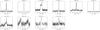 |
Fig. 13 Pulse profiles for the pulsars observed at C-band with the DFB3. Long period, relatively bright pulsars are shown in the top row. The four MSPs are shown in the bottom row. In both rows, the profiles are shown from left to right for increasing pulsar right ascension (i.e. in the same order as presented in Table 9). |
The DFB3 backend performance was initially tested at C band, as this was the lowest available frequency at the time of our first test observations. We preferred C band over K band, as pulsars are expected to be brighter at lower frequencies because of the negative slope of their power spectrum (e.g., Sieber 1973).
The DFB3 produces files in psrfits format (Hotan et al. 2004), hence SRT pulsar data can be directly handled with the most common, available pulsar software (e.g., psrchive19, dspsr20, and presto21). The telescope code in the file headers is SRT. Most pulsar software packages have already been modified to include this code; the tempo22 (Hobbs et al. 2006) one-letter code for our telescope is z and the alias is srt.
Test observations at C band started in June 2013 on a small number of pulsars and continued until the L/P band coaxial receiver was installed. The data acquisition was initially carried out using the built-in TKDS graphical interface, which is now fully superseded by the new data acquisition system named SEADAS (see Sect. 3.2). The backend configurations tested at C band are listed in Table 8. Both folding and search mode observations, with sampling times down to 100 μs, were successfully performed.
We observed six bright long period pulsars and four MSPs for which a flux density measurement at a similar frequency was reported in the literature along with a spectral index (Kramer et al. 1999). Table 9 lists the observed pulsars, along with the main observational details. For each observed pulsar, we report the number of observations performed (Nobs), the average length of each observation (tobs), and the average S/N achieved. Figure 13 shows their integrated pulse profiles.
Pulsars observed at C band.
At the time of these observations, an accurate flux density and polarization calibration was not possible, as the noise diode (which allows the DFB3 to directly switch its signal on and off) was not yet implemented through an optical link. An estimate of the pulsar flux densities at 6 GHz was then calculated from a modification of the radiometer equation for pulsars (see, e.g., Manchester et al. 2001). This estimate is reported in the last column of Table 9 (S6000). Flux densities are broadly consistent (within a factor of ~2–3) with those found in the literature. This discrepancy is not surprising given the inherent approximation of the uncalibrated method used to estimate flux densities (that introduces errors ≳30%) and the fact that we used the (best-case scenario) tabulated value of the system temperature. Nevertheless, our C-band observations allowed us to test and fine-tune the backend and the pulsar acquisition and recording system.
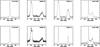 |
Fig. 14 Pulse profiles at 1550 MHz for the four MSPs observed both at C and L bands. The name of each pulsar is written on the top right corner of each panel. The top row shows the pulses as observed with the DFB3, while in the bottom row we show those obtained with the ROACH board. The plots for the two backends are not obtained simultaneously, so the S/N of the two profiles are not directly comparable. We also note that three of these pulsars (all except B1937+21) are heavily affected by interstellar scintillation. |
9.2. Pulsar observations at L band
When the L/P band coaxial receiver was installed and characterized, a very extensive observing campaign started in which we exploited these lower frequencies to observe ~50 known pulsars (taken from the ATNF pulsar catalog23; Manchester et al. 2005) spanning a wide range of periods (from ~1 ms to ~1 s), dispersion measures (from ~3 to ~250 pc/cm3), and 1400 MHz flux densities (from ~40 μJy to ~200 mJy) with all of the available DFB3 configurations for either folding or search observing modes. A subsample was also observed with the ROACH board.
Since our backends have not yet been placed in a screened chamber and the control room itself is still in a temporary location, the RFI situation at these lower frequencies is still largely suboptimal. In addition, an oscillating noise diode was only recently installed for the L/P band receiver, and it is still undergoing tests. Despite these limitations, we were able to make extensive comparison tests of the performance of the DFB3 and ROACH backends.
As test cases, here we present the results obtained for the four MSPs that were also observed at C band. In Table 10 we present the main parameters of these MSPs: spin period (P0), dispersion measure (DM), and, when available, flux density at 1400 MHz (S1400). In Fig. 14, we compare the pulse shapes obtained with the DFB3 and with the ROACH board at L band (central frequency 1550 MHz).
While the DFB3 has, at present, a larger bandwidth (512 MHz versus 128 MHz for the ROACH), the ROACH board allows us to coherently dedisperse the signal, fully correcting for the dispersion delay. The DFB3, on the contrary, is limited by its spectral resolution and cannot remove the intra-channel dispersion. In most cases, this only has a minimal impact, or no impact at all, on the observed profile. In the case of short period pulsars with a high dispersion measure, though, the difference in the results obtained with and without coherent dedispersion is significant. As we can clearly see in the case of B1937+ 21, the intra-channel dispersion smearing in the 1 MHz-wide channel of the DFB3 observation is, at the lower end of the observing band, ~ 17% of the spin period, which is much larger than the intrinsic pulse width correctly recovered by the ROACH observation.
Main parameters of the four MSPs observed at both C and L band with the DFB3 and ROACH backends.
To demonstrate the timing performance of the SRT, in Fig. 15 we compare the times of arrival for the MSP J1022+1001 as measured at the SRT (black) and WSRT (blue). These observations were taken as part of the LEAP project (see Sect. 10 for more details) from March 2014 to January 2016. The measurements from the two telescopes are consistent and the error bars are comparable (taking into account the larger equivalent surface of the WSRT and the currently worse RFI environment at the SRT), proving that the timing capabilities of the SRT are up to standards. The increase in the error bars at the beginning of 2015 (middle of the plot) is due to a combination of effects; on the one hand, the targeted pulsar appeared dimmer because of scintillation; on the other hand, the WSRT was starting to use fewer and fewer dishes for the LEAP project (see Fig. 15 caption for details) and the SRT data suffered from packet loss, causing 8 MHz of bandwidth to become unusable for some of the epochs. After June 2015, WSRT stopped LEAP observations because of the upgrade of the L-band receivers of the majority of the dishes to focal plane array technology (Apertif; Verheijen et al. 2008), and only SRT measurements are available.
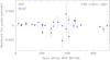 |
Fig. 15 Timing residuals (observed minus predicted times of arrival vs time) for PSR J1022+1001, monthly observed for the LEAP project (Bassa et al. 2016) from March 2014 to January 2016. The black points refer to the SRT and the blue ones to WSRT. We note that the WSRT used 10 dishes in March and April 2014 (for an equivalent size of 75-m), nine from May to August 2014 and eight from September 2014 to January 2015. The number of WSRT dishes available for LEAP observations decreased to seven and then to five (66 to 56-m equivalent size) from February to June 2015, when the last LEAP point at WSRT was taken (Janssen priv. comm.). |
We expect an improvement of a factor of at least two in the S/N of our observations when the local RFI environment at the SRT is mitigated, by placing the equipment backends in a Faraday cage and screening the signals produced by the equipment in the Gregorian focus.
A more complete characterization of the full potential of the SRT for pulsar observations will be presented in a future paper, as soon as the on-site RFI situation is better managed, and the oscillating noise diodes at L and P bands become fully operational.
10. LEAP observations
Starting in July 2013, the SRT joined the LEAP project, a subproject of the EPTA, performing observations of a set of millisecond pulsars simultaneously with the other four radio telescopes of the collaboration, using the L-band receiver and the ROACH backend. The pulsar timing data are reduced locally and the raw baseband data are shipped to Jodrell Bank, where the baseband data from all individual telescopes are correlated to find the phase offsets between the telescopes. The data are then corrected for the offsets and added coherently to form a tied-array beam, obtaining in this way high precision timing data. The high precision timing that is possible with LEAP will in turn be used, over timescales of a minimum of 5–10 yr, to search for GW signatures. The details of the LEAP project and first results are shown in Bassa et al. (2016).
The SRT initially observed in a single 16 MHz sub-band of the LEAP bandwidth (1332–1460 MHz); starting in the spring of 2014, it has performed monthly observations in the full LEAP bandwidth and with the full set of millisecond pulsars (owing to an 8-node CPU cluster and storage computer being installed on site; see Prandoni et al. 2014; Perrodin et al. 2014, 2016, for more details about the setup). In May 2014, we found the first fringe between the SRT and another telescope of the collaboration, the WSRT, using the LEAP correlation software at Jodrell Bank, thus showing the successful addition of the SRT to the LEAP tied array. This is shown in Fig. 16.
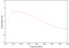 |
Fig. 16 First fringe obtained between SRT and WSRT using the LEAP correlation pipeline: 5-s long observation of the quasar 3C 454 at 1420 MHz (May 2014). |
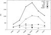 |
Fig. 17 Comparison of the S/N from LEAP coherent additions to the S/N from the individual telescopes for PSR J1022+1001. The observations span the period from February 2012 to February 2015. We note that PSR J1022+1001 is affected by scintillation and its S/N can vary wildly between observations. The SRT is included in MJD 56 945. |
We have now collected over two years of monthly LEAP data at the SRT, improving in this way the S/N of the LEAP data set. In coherent additions, the S/N of pulsar timing signals should increase linearly with the number of telescopes, as opposed to the square root of the number of telescopes in the case of incoherent additions. Of course this is valid if the telescopes are identical in size and performance; in the case of LEAP, the S/N of the coherent sum is expected to be equal to the sum of the S/N of the individual telescopes. In Fig. 17, we show LEAP coherent sums for PSR J1022+1001 (from Bassa et al. 2016). The SRT is included in one epoch (MJD 56 945), where it contributes roughly the same level of S/N as the WSRT to the combined LEAP S/N. This confirms the comparison between SRT and the WSRT that is shown in Fig. 15. We expect that the S/N of LEAP observations at SRT will continue to increase as most sources of RFI are identified and mitigated.
11. Target of opportunity observations
Since 2013, the SRT has been made available to the international community for ToO observations on a best effort basis, as part of the AV activities. The primary targets of SRT ToOs have been transient magnetars after X-ray outbursts and FRBs.
The ToO program was kicked off on May 6, 2013, internally by the AV team, with observations of the transient magnetar SGR J1745-2900. This peculiar source, showing a 3.67 s period pulsation, was discovered only a few days earlier by the NuSTAR X-ray telescope in the vicinity of the Galactic center (Mori et al. 2013). Despite the fact that the L/P band receiver and the DFB3 and ROACH backends designed for pulsar observations were not yet installed at the time, the SRT successfully detected radio pulsations from the magnetar for the first time at upper C band (Buttu et al. 2013) through observations performed with the TP backend, sampled every 40 ms over a bandwidth of 680 MHz. This was possible thanks to the peculiar characteristics of radio magnetars (long periods and roughly flat radio spectra) and to the prompt development (by members of the AV team) of an ad-hoc software tool able to fold the TP data using the X-ray rotational ephemerides for the magnetar and optimize the spin period to obtain maximum S/N for the pulsed profile (Fig. 18). This 7.3 GHz observation, whose estimated flux density is 0.1 mJy (Buttu et al. 2013), nicely complements the detections at 8 and 5 GHz performed at the Effelsberg radio telescope, where radio pulsations of the magnetar were first discovered (Eatough et al. 2013a,b).
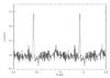 |
Fig. 18 Pulse profile at 7.3 GHz for SGR J1745-2900 folded with the period obtained by Swift (Gotthelf et al. 2013) and refined to maximize the S/N. |
Main observational parameters for SGR (top) and FRB (bottom) ToOs at the SRT.
Other examples of transients followed up at the SRT are SGR J1935+2154 (Israel et al. 2014), SGR J0755-2933 (Barthelmy et al. 2016) and the magnetar candidate SGR J1819-1600 (Mereghetti et al. 2012; Page et al. 2015).
A Letter of Intent was signed on January 13, 2015, which included the SRT in the follow-up observations of FRB discoveries from the SUPERB (SUrvey for Pulsar and Extragalactic Radio Bursts) project (Keane et al., in prep.). As part of this agreement, the SRT performed L-band and P-band follow-up observations of FRB150418 (Keane et al. 2016), FRB151206, FRB151230, and FRB160102 (Bhandari et al., in prep.) promptly after receiving a trigger from the SUPERB collaboration. With the detection by Spitler et al. (2016) of repeating occurrences of pulses from FRB121102 (Spitler et al. 2014), further observations of FRB151206, FRB151230, and FRB160102 were performed at L band and P band, while FRB121102 was observed at C band for six hours. No single pulses around the discovery dispersion measure of the FRBs were detected in the data.
The main observational details of both SGRs and FRBs observed at the SRT as ToOs are listed in Table 11. For each source, we list the date of the observation (in YYYYMMDD format), central observing frequency in GHz (νobs), total bandwidth in MHz (BW), frequency resolution in MHz (Δν), time resolution in μsec (tsampl), backend used, and observation length (tobs). The last column lists the measured flux density or upper limit (S; in mJy for SGRs and in Jy for FRBs). For FRB flux density estimates, we explicitly indicate the dependence on the pulse duration W (normalized over the actual duration of the observed pulse, in ms). This allows us to take into account pulse width variations that may occur in following burst episodes.
Several other ToOs have been triggered at the SRT on a variety of types of astronomical objects, from comets to ultra-luminous X-ray sources to GRBs (see, e.g., Nappo et al. 2016; Egron et al. 2017a). A full description of such observations is beyond the scope of this paper and we refer to the literature for more details.
12. Summary
In this paper, we have provided a brief overview of the SRT and the science applications envisaged for it. We then reported the main results of its AV, which was carried out in the period 2012–2015.
The AV activities started during the technical commissioning of the telescope when several external software tools were developed to assist the preparation, execution, and monitoring of the observations along with the data inspection and reduction. This suite of astronomer-oriented software tools are meant to support future observers on site.
The scientific commissioning of the SRT, based on first-light receivers and backends, then proceeded in steps, from basic on-sky tests aimed at verifying the general performance and/or the limits of the telescope and the acquisition systems, to more complex acquisitions aimed at assessing the actual SRT capabilities for a range of scientific observations.
The activities were prioritized based on technical readiness and scientific impact. Highest priority was given to make the SRT available for joint observations as part of European networks: the EVN and the LEAP.
After the first successful VLBI data correlation of the Medicina–SRT baseline in January 2014 and the following EVN test observations (see Prandoni et al. 2014), the SRT was offered as an additional EVN station in shared-risk mode for all of its three first-light observing bands (L, C, and K bands), starting from 2015.
In parallel, all of the hardware and software necessary for the LEAP project was developed and installed at the SRT, where it was fully tested and debugged. Since early 2014, the SRT participates in monthly LEAP runs, for which data acquisition is now fully automated. The first results of the LEAP project, including the SRT, are presented in Bassa et al. (2016).
The validation of single-dish operations for the suite of SRT first light receivers and backends continued until the end of 2015, when the SRT capabilities for imaging, spectroscopy, and pulsar observations were demonstrated. In this paper, we highlighted in particular the superb imaging performance of the SRT, both in terms of dynamic range and image fidelity.
Since 2013, a ToO program is offered to the community on a best-effort basis. The ToO program was kicked off with the follow-up observation of the transient magnetar SGR J1745-2900, which was detected at the SRT at 7.3 GHz (Buttu et al. 2013). In January 2015, the SRT was included in the agreement for follow-up observations of FRB discoveries from the SUPERB project (Keane et al., in prep.). A formal agreement has also been established to include the SRT in a large multiwavelength program aimed to identify and initially follow up the electromagnetic counterparts of GW events.
The AV activity was formally concluded with the first call for shared-risk, early-science observations issued at the end of 2015. Early science observations started on February 1, 2016 and were conducted for a period of six months. These observations are aimed at further demonstrating the scientific potential of the SRT and several papers are expected to appear in the literature based on early science observations.
Details about the time allocation procedures and policy will be released at a suitable time before the beginning of each observing term.
In the future, two more BWG focal positions will be implemented for space science applications.
The HPBW (in arcmin) roughly scales as k/ν, where k is a RF-band dependent constant and ν is the frequency (in GHz): k = 19.590 for P band; k = 19.373 for L band; 18.937 for C band; k = 18.264 for K band.
Collaboration for Astronomy Signal Processing and Electronics Research.
Acronym for SArdinia Roach2-based Digital Architecture for Radio Astronomy.
On-Off position switching is an observing mode typically used for spectroscopic observations. It corresponds to alternate on-source/off-source pointing sequences. The off-source spectrum is used to remove atmospheric and system noise, and to bandpass calibrate the on-source spectrum.
On-the-Fly cross-scans (or simply cross-scans) are fast acquisitions carried out along two orthogonal directions, usually coinciding with the axes of a celestial coordinate frame. They are mainly employed to observe point-like sources, in order to ultimately measure their flux density and position. Cross-scans allow an accurate estimate of the source peak position, in turn permitting us to correct for pointing errors (local residuals with respect to the pointing model).
Raster scans are sequences of pointed acquisitions organized in grids, mainly used to sample discrete portions of extended targets according to a pre-defined geometry.
OTF mapping is an observing mode exploiting fast OTF scans across a given area. Scans are properly weaved and interspaced, in order to achieve the requested sampling in the final map.
CASTIA means “look” in Sardinian.
The phenomenon of standing waves is caused by multiple internal reflections between the primary and secondary mirrors. Standing waves produce periodic ripples in the observed spectra and are particularly detrimental to wide-band spectroscopic observations. A shaped Gregorian optical configuration produces a null field in the region blocked by the subreflector, thereby significantly mitigates this phenomenon.
We used the new PCCALS4.7 version, kindly provided to us by J. Condon.
We used a Leica Absolute Tracker AT402 model.
We adopted the same rest frequency as used by Knowles et al. (1976) to better compare our spectra to those shown in their Fig. 9, which have a similar spectral resolution (0.06 km s-1).
Acknowledgments
The Astronomical Validation activities were made possible thanks to the invaluable support of the local technical staff and the technical commissioning team. The authors thank Cees Bassa and Ramesh Karuppusamy for their important help in setting up the ROACH backend for pulsar observations. D. Perrodin thanks Gemma Janssen for providing WSRT timing residuals shown in Fig. 15. F. Loi gratefully acknowledges the Sardinia Regional Government for financial support of her PhD scholarship (P.O.R. Sardegna F.S.E. Operational Programme of the Autonomous Region of Sardinia, European Social Fund 2007–2013 – Axis IV Human Resources, Objective l.3, Line of Activity l.3.1.). From 2012 to 2014, D. Perrodin was supported by the ERC Advanced Grant “LEAP”, Grant Agreement Number 227947 (PI M. Kramer), which also provided a 10-gigabit-ethernet switch and a storage cluster for SRT LEAP observations. M. Pilia was supported by the Sardinia Regional Government through the project “Development of a Software Tool for the Study of Pulsars from Radio to Gamma-rays using Multi-mission Data” (CRP-25476). A. Ridolfi and C. Tiburzi gratefully acknowledge support from the Max-Planck-Institut für Radioastronomie. C.Tiburzi also acknowledges support from the Universitaet Bielefeld. V. Vacca was supported by the DFG Forschengruppe 1254 “Magnetisation of Interstellar and Intergalactic Media: The Prospects of Low-Frequency Radio Observations”. The development of the SARDARA backend was funded by the Autonomous Region of Sardinia (RAS) using resources from the Regional Law 7/2007 “Promotion of the scientific research and technological innovation in Sardinia” in the context of the research project CRP-49231 (year 2011): “High resolution sampling of the Universe in the radio band: an unprecedented instrument to understand the fundamental laws of the nature”. The Sardinia Radio Telescope is funded by the Department of University and Research (MIUR), the Italian Space Agency (ASI), and the Autonomous Region of Sardinia (RAS). It is operated as national facility by the National Institute for Astrophysics (INAF).
References
- Abbott, B. P., Abbott, R., Abbott, T. D., et al. 2016, Phys. Rev. Lett., 116, 061102 [Google Scholar]
- AMI Consortium, Davies, M. L., Franzen, T. M. O., Waldram, E. M., et al. 2011, MNRAS, 415, 2708 [NASA ADS] [CrossRef] [Google Scholar]
- Baars, J. W. M., Genzel, R., Pauliny-Toth, I. I. K., & Witzel, A. 1977, A&A, 61, 99 [NASA ADS] [Google Scholar]
- Bagdonaite, J., Jansen, P., Henkel, C., et al. 2013, Science, 339, 46 [NASA ADS] [CrossRef] [Google Scholar]
- Barthelmy, S. D., D’Elia, V., Gehrels, N., et al. 2016, ATel, 8831 [Google Scholar]
- Bartolini, M., & Righini, S. 2016, IRA Technical Report, IRA 492/16 [Google Scholar]
- Bartolini, M., Libardi, P., & Righini, S. 2013, IRA Technical Report, IRA 466/13 [Google Scholar]
- Bassa, C. G., Janssen, G. H., Karuppusamy, R., et al. 2016, MNRAS, 456, 2196 [NASA ADS] [CrossRef] [Google Scholar]
- Baudry, A., Desmurs, J. F., Wilson, T. L., & Cohen, R. J. 1997, A&A, 325, 255 [NASA ADS] [Google Scholar]
- Bolli, P., Olmi, L., Roda, J., & Zacchiroli, G. 2014, IEEE Antennas Propag. Lett., 13, 1713 [NASA ADS] [CrossRef] [Google Scholar]
- Bolli, P., Orlati, A., Stringhetti, L., et al. 2015, J. Astron. Instrum., 4, 1550008 [CrossRef] [Google Scholar]
- Braun, R., & Strom, R. G. 1986, A&A, 164, 193 [NASA ADS] [Google Scholar]
- Brunthaler, A., Reid, M. J., Falcke, H., Greenhill, L. J., & Henkel, C. 2005, Science, 307, 1440 [NASA ADS] [CrossRef] [PubMed] [Google Scholar]
- Brunthaler, A., Reid, M. J., Falcke, H., Henkel, C., & Menten, K. M. 2007, A&A, 462, 101 [NASA ADS] [CrossRef] [EDP Sciences] [Google Scholar]
- Buffa, F., Serra, G., Bolli, P., et al. 2016, OAC Internal Report, 54 [Google Scholar]
- Buttu, M., Orlati, A., Zacchiroli, G., et al. 2012, in Software and Cyberinfrastructure for Astronomy II, Proc. SPIE, 8451, 84512 [CrossRef] [Google Scholar]
- Buttu, M., D’Amico, N., Egron, E., et al. 2013, ATel, 5053 [Google Scholar]
- Carilli, C. L., & Taylor, G. B. 2002, ARA&A, 40, 319 [NASA ADS] [CrossRef] [Google Scholar]
- Carretti, E., Crocker, R. M., Staveley-Smith, L., et al. 2013, Nature, 493, 66 [NASA ADS] [CrossRef] [PubMed] [Google Scholar]
- Caswell, J. L., & Vaile, R. A. 1995, MNRAS, 273, 328 [NASA ADS] [CrossRef] [Google Scholar]
- Chatterjee, S., Law, C. J., Wharton, R. S., et al. 2017, Nature, 541, 58 [NASA ADS] [CrossRef] [Google Scholar]
- Condon, J. J. 2009, PTCS Project Note, 66.0 [Google Scholar]
- Corongiu, A. 2014, OAC Internal Report, 35 [Google Scholar]
- de Gasperin, F., Orrú, E., Murgia, M., et al. 2012, A&A, 547, A56 [NASA ADS] [CrossRef] [EDP Sciences] [Google Scholar]
- Deller, A. T., Tingay, S. J., Bailes, M., & West, C. 2007, PASP, 119, 318 [NASA ADS] [CrossRef] [Google Scholar]
- Eatough, R., Karuppusamy, R., Kramer, M., et al. 2013a, ATel, 5043 [Google Scholar]
- Eatough, R., Karuppusamy, R., Kramer, M., et al. 2013b, ATel, 5040 [Google Scholar]
- Egron, E., Pellizzoni, A., Iacolina, N. M., et al. 2016, OAC Internal Report, 59 [Google Scholar]
- Egron, E., Pellizzoni, A., Giroletti, M., et al. 2017a, MNRAS, 471, 2703 [NASA ADS] [CrossRef] [Google Scholar]
- Egron, E., Pellizzoni, A., Iacolina, N. M., et al. 2017b, MNRAS, 470, 1329 [NASA ADS] [CrossRef] [Google Scholar]
- Fender, R., & Gallo, E. 2014, Space Sci. Rev., 183, 323 [NASA ADS] [CrossRef] [Google Scholar]
- Feretti, L., Giovannini, G., Govoni, F., & Murgia, M. 2012, A&ARv, 20, 54 [Google Scholar]
- Ferrari, C., Govoni, F., Schindler, S., Bykov, A. M., & Rephaeli, Y. 2008, Space Sci. Rev., 134, 93 [NASA ADS] [CrossRef] [Google Scholar]
- Fish, V. L., Reid, M. J., Menten, K. M., & Pillai, T. 2006, A&A, 458, 485 [NASA ADS] [CrossRef] [EDP Sciences] [Google Scholar]
- Gao, X. Y., Han, J. L., Reich, W., et al. 2011, A&A, 529, A159 [NASA ADS] [CrossRef] [EDP Sciences] [Google Scholar]
- Gebhardt, K., & Thomas, J. 2009, ApJ, 700, 1690 [NASA ADS] [CrossRef] [Google Scholar]
- Gedalin, M., & Eichler, D. 1993, ApJ, 406, 629 [NASA ADS] [CrossRef] [Google Scholar]
- Gotthelf, E. V., Mori, K., Halpern, J. P., et al. 2013, ATel, 5046 [Google Scholar]
- Govoni, F., & Feretti, L. 2004, Int. J. Mod. Phys. D, 13, 1549 [NASA ADS] [CrossRef] [Google Scholar]
- Govoni, F., Murgia, M., Vacca, V., et al. 2017, A&A, 603, A122 [NASA ADS] [CrossRef] [EDP Sciences] [Google Scholar]
- Green, D. A. 2014, BASI, 42, 47 [Google Scholar]
- Grueff, G., Alvito, G., Ambrosini, R., et al. 2004, in Ground-based Telescopes, ed. J. M. Oschmann, Jr., Proc. SPIE, 5489, 773 [NASA ADS] [CrossRef] [Google Scholar]
- Heiles, C. 1984, ApJS, 55, 585 [NASA ADS] [CrossRef] [Google Scholar]
- Heiles, C. 1996, ApJ, 466, 224 [NASA ADS] [CrossRef] [Google Scholar]
- Heiles, C., Perillat, P., Nolan, M., et al. 2001, PASP, 113, 1274 [NASA ADS] [CrossRef] [Google Scholar]
- Hobbs, G. 2013, Class. Quant. Grav., 30, 224007 [Google Scholar]
- Hobbs, G. B., Edwards, R. T., & Manchester, R. N. 2006, MNRAS, 369, 655 [NASA ADS] [CrossRef] [Google Scholar]
- Hotan, A. W., van Straten, W., & Manchester, R. N. 2004, PASA, 21, 302 [NASA ADS] [CrossRef] [Google Scholar]
- Israel, G. L., Rea, N., Zelati, F. C., et al. 2014, ATel, 6370 [Google Scholar]
- Kanekar, N., Ubachs, W., Menten, K. M., et al. 2015, MNRAS, 448, L104 [NASA ADS] [CrossRef] [Google Scholar]
- Keane, E. F., Johnston, S., Bhandari, S., et al. 2016, Nature, 530, 453 [NASA ADS] [CrossRef] [Google Scholar]
- Khechinashvili, D. G., Melikidze, G. I., & Gil, J. A. 2000, ApJ, 541, 335 [NASA ADS] [CrossRef] [Google Scholar]
- Knowles, S. H., Caswell, J. L., & Goss, W. M. 1976, MNRAS, 175, 537 [NASA ADS] [CrossRef] [Google Scholar]
- Kramer, M., & Champion, D. J. 2013, Class. Quant. Grav., 30, 224009 [Google Scholar]
- Kramer, M., Lange, C., Lorimer, D. R., et al. 1999, ApJ, 526, 957 [NASA ADS] [CrossRef] [Google Scholar]
- Lee, J.-J., Koo, B.-C., Yun, M. S., et al. 2008, AJ, 135, 796 [NASA ADS] [CrossRef] [Google Scholar]
- Manchester, R. N., & IPTA. 2013, Class. Quant. Grav., 30, 224010 [NASA ADS] [CrossRef] [Google Scholar]
- Manchester, R. N., Lyne, A. G., Camilo, F., et al. 2001, MNRAS, 328, 17 [NASA ADS] [CrossRef] [Google Scholar]
- Manchester, R. N., Hobbs, G. B., Teoh, A., & Hobbs, M. 2005, AJ, 129, 1993 [NASA ADS] [CrossRef] [Google Scholar]
- Massardi, M., Ekers, R. D., Murphy, T., et al. 2011, MNRAS, 412, 318 [NASA ADS] [CrossRef] [Google Scholar]
- McLaughlin, M. A. 2013, Class. Quant. Grav., 30, 224008 [Google Scholar]
- McLaughlin, M. A., Lyne, A. G., Lorimer, D. R., et al. 2006, Nature, 439, 817 [NASA ADS] [CrossRef] [PubMed] [Google Scholar]
- Melis, A., Concu, R., Trois, A., et al. 2014a, OAC Internal Report, 36 [Google Scholar]
- Melis, A., Gaudiomonte, F., Barbaro, M., et al. 2014b, in Millimeter, Submillimeter, and Far-Infrared Detectors and Instrumentation for Astronomy VII, Proc. SPIE, 9153, 915338 [CrossRef] [Google Scholar]
- Melis, A., Valente, G., Tarchi, A., et al. 2014c, in Millimeter, Submillimeter, and Far-Infrared Detectors and Instrumentation for Astronomy VII, Proc. SPIE, 9153, 91532M [CrossRef] [Google Scholar]
- Melis, A., Migoni, C., Comoretto, G., et al. 2015, OAC Internal Report, 52 [Google Scholar]
- Melis, A., Concu, R., Trois, A., et al. 2017, J. Astron. Instrum., submitted [Google Scholar]
- Menten, K. M. 1991, ApJ, 380, L75 [NASA ADS] [CrossRef] [Google Scholar]
- Mereghetti, S., Esposito, P., Tiengo, A., et al. 2012, A&A, 546, A30 [NASA ADS] [CrossRef] [EDP Sciences] [Google Scholar]
- Merloni, A., Heinz, S., & di Matteo, T. 2003, MNRAS, 345, 1057 [NASA ADS] [CrossRef] [Google Scholar]
- Migoni, C., Melis, A., Fara, A., et al. 2014, OAC Internal Report, 42 [Google Scholar]
- Mori, K., Gotthelf, E. V., Barriere, N. M., et al. 2013, ATel, 5020 [Google Scholar]
- Murgia, M. 2011, Mem. Soc. Astron. Ital., 82, 507 [NASA ADS] [Google Scholar]
- Murgia, M., Govoni, F., Feretti, L., et al. 2004, A&A, 424, 429 [NASA ADS] [CrossRef] [EDP Sciences] [Google Scholar]
- Murgia, M., Govoni, F., Carretti, E., et al. 2016, MNRAS, 461, 3516 [NASA ADS] [CrossRef] [Google Scholar]
- Murphy, T., Sadler, E. M., Ekers, R. D., et al. 2010, MNRAS, 402, 2403 [NASA ADS] [CrossRef] [Google Scholar]
- Nappo, F., Pescalli, A., Oganesyan, G., et al. 2017, A&A, 598, A23 [NASA ADS] [CrossRef] [EDP Sciences] [Google Scholar]
- Nasir, F. T., Castiglia, C., Buffa, F., et al. 2013, Exp. Astron., 36, 407 [NASA ADS] [CrossRef] [Google Scholar]
- Olbert, C. M., Clearfield, C. R., Williams, N. E., Keohane, J. W., & Frail, D. A. 2001, ApJ, 554, L205 [NASA ADS] [CrossRef] [Google Scholar]
- Orlati, A., Buttu, M., Melis, A., et al. 2012, in Software and Cyberinfrastructure for Astronomy II, Proc. SPIE, 8451, 84512M [CrossRef] [Google Scholar]
- Orlati, A., Bartolini, M., Buttu, M., et al. 2015, in Proceedings 15th International Conference on Accelerator and Large Experimental Physics Control Systems (ICALEPCS 2015): Melbourne, Australia, October 17–23, 2015, MOPGF110 [Google Scholar]
- Owen, F. N., Eilek, J. A., & Kassim, N. E. 2000, ApJ, 543, 611 [NASA ADS] [CrossRef] [Google Scholar]
- Page, K. L., Barthelmy, S., & Cummings, J. R. 2015, GRB Coordinates Network, 18632 [Google Scholar]
- Perley, R. A., & Butler, B. J. 2013, ApJS, 204, 19 [NASA ADS] [CrossRef] [Google Scholar]
- Perrodin, D., Bassa, C. G., Janssen, G. H., et al. 2016, in Proceedings of the 14th Marcel Grossmann Meeting on General Relativity (MG 14), Rome, 2015, in press [arXiv:1608.01839] [Google Scholar]
- Perrodin, D., Concu, R., Melis, A., et al. 2014, OAC Internal Report, 39 [Google Scholar]
- Phinney, E. S., Evans, C. R., Blandford, R. D., & Kulkarni, S. R. 1988, Nature, 333, 832 [NASA ADS] [CrossRef] [Google Scholar]
- Prandoni, I., Melis, A., Migoni, C., et al. 2014, in Proceedings of the 12th European VLBI Network Symposium and Users Meeting (EVN 2014), 7–10 October 2014, Cagliari, Italy, 46 [Google Scholar]
- Prestage, R. M., & Maddalena, R. J. 2003, in Large Ground-based Telescopes, eds. J. M. Oschmann & L. M. Stepp, Proc. SPIE, 4837, 944 [Google Scholar]
- Rasio, F. A., Shapiro, S. L., & Teukolsky, S. A. 1989, ApJ, 342, 934 [NASA ADS] [CrossRef] [Google Scholar]
- Rasio, F. A., Shapiro, S. L., & Teukolsky, S. A. 1991, A&A, 241, L25 [NASA ADS] [Google Scholar]
- Reid, M. J., Braatz, J. A., Condon, J. J., et al. 2013, ApJ, 767, 154 [NASA ADS] [CrossRef] [Google Scholar]
- Ricci, R., Righini, S., Verma, R., et al. 2013, MNRAS, 435, 2793 [NASA ADS] [CrossRef] [Google Scholar]
- Ricci, R., Tarchi, A., Poppi, S., et al. 2016, IRA Internal Report, IRA 496/16 [Google Scholar]
- Rickard, L. J., Palmer, P., & Zuckerman, B. 1975, ApJ, 200, 6 [NASA ADS] [CrossRef] [Google Scholar]
- Righini, S., Carretti, E., Ricci, R., et al. 2012, MNRAS, 426, 2107 [NASA ADS] [CrossRef] [Google Scholar]
- Rottmann, H., Mack, K.-H., Klein, U., & Wielebinski, R. 1996, A&A, 309, L19 [NASA ADS] [Google Scholar]
- Sieber, W. 1973, A&A, 28, 237 [NASA ADS] [Google Scholar]
- Spitler, L. G., Cordes, J. M., Hessels, J. W. T., et al. 2014, ApJ, 790, 101 [NASA ADS] [CrossRef] [Google Scholar]
- Spitler, L. G., Scholz, P., Hessels, J. W. T., et al. 2016, Nature, 531, 202 [NASA ADS] [CrossRef] [Google Scholar]
- Stappers, B. W., Bailes, M., Lyne, A. G., et al. 2001, MNRAS, 321, 576 [NASA ADS] [CrossRef] [Google Scholar]
- Tarchi, A., Castangia, P., Govoni, F., et al. 2013, OAC Internal Report, 27 [Google Scholar]
- Thompson, C., Blandford, R. D., Evans, C. R., & Phinney, E. S. 1994, ApJ, 422, 304 [Google Scholar]
- Thornton, D., Stappers, B., Bailes, M., et al. 2013, Science, 341, 53 [NASA ADS] [CrossRef] [PubMed] [Google Scholar]
- Tofani, G., Alvito, G., Ambrosini, R., et al. 2008, in Ground-based and Airborne Telescopes II, Proc. SPIE, 7012, 70120F [CrossRef] [Google Scholar]
- Vacca, V., Iacolina, M. N., Pellizzoni, A., et al. 2013, IRA Internal Report, IRA 468/13 [Google Scholar]
- Verheijen, M. A. W., Oosterloo, T. A., van Cappellen, W. A., et al. 2008, in The Evolution of Galaxies Through the Neutral Hydrogen Window, eds. R. Minchin, & E. Momjian, AIP Conf. Ser., 1035, 265 [Google Scholar]
- Vigotti, M., Gregorini, L., Klein, U., & Mack, K.-H. 1999, A&AS, 139, 359 [NASA ADS] [CrossRef] [EDP Sciences] [Google Scholar]
- Vlemmings, W. H. T. 2008, A&A, 484, 773 [NASA ADS] [CrossRef] [EDP Sciences] [Google Scholar]
- Zanichelli, A., Righini, S., Mack, K.-H., Orfei, A., & Vacca, V. 2015, IRA Technical Report, IRA 487/15 [Google Scholar]
All Tables
Statistics of the positional offset and source FWHM for candidate pointing calibrators.
Observational details of the SRT beam characterization campaigns at C and K bands using the TP backend.
Line parameters of the excited-state OH maser toward the ultra-compact HII region M17-UC1 in the Omega Nebula.
Main parameters of the four MSPs observed at both C and L band with the DFB3 and ROACH backends.
All Figures
|
Fig. 1 C-band Jansky-to-counts conversion factor as measured for different calibrators in four observing sessions (separated by dashed vertical lines), spread over a 10-month timescale. Different colors correspond to different calibrators, as labeled in the panel. The dashed horizontal lines indicate the ± 0.002 rms variations around the average value of 0.06. For each observing session we report the date of the observations. |
| In the text | |
|
Fig. 2 SRT beam patterns at C-band (7.24 GHz, left-column panels) and K-band (right-column panels) respectively. For K-band we show only the 25.54 GHz measurement of the central beam. Top: elevation-averaged beam patterns (normalized to a peak value of 1) obtained by stacking together several OTF scans of bright point sources taken at different elevations. The color map has been intentionally saturated to highlight the low intensity features of the second and third lobes. Bottom: beam cross-sections along the azimuth and elevation axes (in dB). |
| In the text | |
|
Fig. 3 Variation of the SRT beam pattern at 7.24 GHz as a function of elevation. Each image shows a field of view of 6′ × 6′ centered on the beam pattern peak (normalized to 1). Contour levels start at −25 dB and increase by 1 dB. |
| In the text | |
|
Fig. 4 Gain (in K/Jy) as a function of elevation measured through OTF scans at 7.24 GHz (left panels) and at 25.54 GHz (right panels), with a bandwidth of 680 MHz. The right and left polarizations are shown separately (top and bottom panels respectively). The solid lines represent fourth order polynomial fits. The 25.54 GHz gain curve refers to the central feed of the K-band receiver. |
| In the text | |
|
Fig. 5 Source (baseline-subtracted) amplitude vs. peak (source + baseline) level, both expressed in raw counts. Increasing raw counts on both axes reflect decreasing attenuation. Top panel: illustration of the test performed with 250 MHz bandwidth at a central observing frequency of 7.25 GHz. Different sources are indicated by different colors, as labeled in the panel. Bottom panel: illustration of the test performed with 1200 MHz bandwidth at a central observing frequency of 6.8 GHz. Here only the bright source 3C 286 (5.87 Jy at 6.8 GHz, Perley & Butler 2013) is shown, to highlight the levels of raw counts where saturation is reached. |
| In the text | |
|
Fig. 6 Ratio of measured over expected noise as a function of sampling interval for different bandwidths (blue circles = 250 MHz, green squares = 680 MHz, and red diamonds = 1200 MHz). The noise RMS is measured (and estimated) over different time windows. Here we show the results for 2 s (top) and 4 s (bottom) time windows. The experiment was performed at both C (left panels) and K band (right panels). |
| In the text | |
|
Fig. 7 Measured RMS noise as a function of integration time. The oblique solid line shows the expected trend according to the radiometer equation. The parallel dot-dashed line corresponds to the theoretical noise increased by 25%. The horizontal dot-dashed line shows the measured confusion limit. |
| In the text | |
|
Fig. 8 Left panel: “Dirty” image of Virgo A resulting from the combination of 10 OTF scans achieved with the multi-feed K-band array at a frequency of 19 GHz and a bandwidth of 2 GHz. Close to the source the dynamic range is limited to ~ 30, due to the strong secondary lobes. Right panel: CLEANed image restored with a circular Gaussian with FWHM of 57′′. The measured surface brightness RMS sensitivity is now 1.3 mJy/beam and the dynamic range increases to 11 300. In both panels, contours start from 3σ and increase by a factor of |
| In the text | |
|
Fig. 9 Continuum image of the Omega Nebula obtained with the SRT at 7.24 GHz. The source emission shown extends over about a 1o × 1o region. The RMS noise is ≃7 mJy/beam and the SRT resolution is 2.6 arcmin (SRT beam size at 7.24 GHz). The color map was biased to highlight the low surface brightness emission. As a result, the central and brightest part of the nebula (M17-UC1), characterized by a surface brightness in the range ≃3–100 Jy/beam, is saturated. Inset spectrum:6035 MHz OH maser emission (Jy) observed toward M17-UC1 is shown. Left and right circular polarizations are indicated in yellow and green, respectively. The spectrum was acquired with XARCOS, pointing at the position (J2000) RA = |
| In the text | |
|
Fig. 10 Continuum image of W3 obtained at 7.24 GHz with the SRT. The field of view is about 2o × 2o. The RMS noise is ≃4 mJy/beam and the resolution is 2.6 arcmin (SRT beam size at 7.24 GHz). The color map has been saturated to highlight the low surface brightness emission. Inset spectrum: 6.7 GHz methanol maser emission (Jy) in W3OH is shown. The spectra were taken with XARCOS on January 28, 2016. Four sub-bands (see panels) were observed simultaneously at increasing spectral resolution. Specifically we show spectra with 1.4 km s-1, 170, 40, and 10 m s-1 channel widths (from top to bottom). Left and right circular polarizations have been averaged. The velocity scale refers to the LSR frame and uses the optical convention (for more details see Sect. 8). |
| In the text | |
|
Fig. 11 Comparison of GBT (left panels) and SRT (right panels) images of the Omega Nebula (top) and W3(OH) (bottom). The GBT commissioning observations of the Omega Nebula and of W3 were obtained at 8.4 GHz (Prestage & Maddalena 2003) and 8.9 GHz (GBT site), respectively. |
| In the text | |
|
Fig. 12 Images of SNR IC443. Left: single-dish 7.24 GHz calibrated image obtained with the SRT (2.7′ resolution; image RMS ~ 10 mJy/beam for an effective exposure time of 6.5 h). Right: 1.4 GHz continuum 7-pointing mosaic obtained with the VLA (40′′ resolution) in combination with Arecibo (3.9′ resolution) data to provide sensitivity to extended low surface brightness emission (total observing time 6.3 h). The blue arrows indicate the position of two extra-galactic background sources, and the black arrow indicates the neutron star (from Lee et al. 2008). |
| In the text | |
|
Fig. 13 Pulse profiles for the pulsars observed at C-band with the DFB3. Long period, relatively bright pulsars are shown in the top row. The four MSPs are shown in the bottom row. In both rows, the profiles are shown from left to right for increasing pulsar right ascension (i.e. in the same order as presented in Table 9). |
| In the text | |
|
Fig. 14 Pulse profiles at 1550 MHz for the four MSPs observed both at C and L bands. The name of each pulsar is written on the top right corner of each panel. The top row shows the pulses as observed with the DFB3, while in the bottom row we show those obtained with the ROACH board. The plots for the two backends are not obtained simultaneously, so the S/N of the two profiles are not directly comparable. We also note that three of these pulsars (all except B1937+21) are heavily affected by interstellar scintillation. |
| In the text | |
|
Fig. 15 Timing residuals (observed minus predicted times of arrival vs time) for PSR J1022+1001, monthly observed for the LEAP project (Bassa et al. 2016) from March 2014 to January 2016. The black points refer to the SRT and the blue ones to WSRT. We note that the WSRT used 10 dishes in March and April 2014 (for an equivalent size of 75-m), nine from May to August 2014 and eight from September 2014 to January 2015. The number of WSRT dishes available for LEAP observations decreased to seven and then to five (66 to 56-m equivalent size) from February to June 2015, when the last LEAP point at WSRT was taken (Janssen priv. comm.). |
| In the text | |
|
Fig. 16 First fringe obtained between SRT and WSRT using the LEAP correlation pipeline: 5-s long observation of the quasar 3C 454 at 1420 MHz (May 2014). |
| In the text | |
|
Fig. 17 Comparison of the S/N from LEAP coherent additions to the S/N from the individual telescopes for PSR J1022+1001. The observations span the period from February 2012 to February 2015. We note that PSR J1022+1001 is affected by scintillation and its S/N can vary wildly between observations. The SRT is included in MJD 56 945. |
| In the text | |
|
Fig. 18 Pulse profile at 7.3 GHz for SGR J1745-2900 folded with the period obtained by Swift (Gotthelf et al. 2013) and refined to maximize the S/N. |
| In the text | |
Current usage metrics show cumulative count of Article Views (full-text article views including HTML views, PDF and ePub downloads, according to the available data) and Abstracts Views on Vision4Press platform.
Data correspond to usage on the plateform after 2015. The current usage metrics is available 48-96 hours after online publication and is updated daily on week days.
Initial download of the metrics may take a while.