| Issue |
A&A
Volume 606, October 2017
|
|
|---|---|---|
| Article Number | A58 | |
| Number of page(s) | 14 | |
| Section | Stellar structure and evolution | |
| DOI | https://doi.org/10.1051/0004-6361/201730967 | |
| Published online | 10 October 2017 | |
Activity cycles in members of young loose stellar associations⋆
1 INAF–Osservatorio Astrofisico di Catania via S. Sofia, 78, 95123 Catania, Italy
e-mail: This email address is being protected from spambots. You need JavaScript enabled to view it.
2 University of Catania, Astrophysics Section, Dept. of Physics and Astronomy via S. Sofia, 78, 95123 Catania, Italy
3 Leibniz-Institut für Astrophysik Potsdam (AIP) An der Sternwarte 16, 14482 Potsdam, Germany
Received: 10 April 2017
Accepted: 21 June 2017
Abstract
Context. Magnetic cycles analogous to the solar cycle have been detected in tens of solar-like stars by analyzing long-term time series of different magnetic activity indexes. The relationship between the cycle properties and global stellar parameters is not fully understood yet. One reason for this is the lack of long-term time series for stars covering a wide range of stellar parameters.
Aims. We searched for activity cycles in a sample of 90 young solar-like stars with ages between 4 and 95 Myr with the aim to investigate the properties of activity cycles in this age range.
Methods. We measured the length Pcyc of a given cycle by analyzing the long-term time series of three different activity indexes: the period of rotational modulation, the amplitude of the rotational modulation and the median magnitude in the V band. For each star, we also computed the global magnetic activity index ⟨ IQR ⟩ that is proportional to the amplitude of the rotational modulation and can be regarded as a proxy of the mean level of the surface magnetic activity.
Results. We detected activity cycles in 67 stars. Secondary cycles were also detected in 32 stars of the sample. The lack of correlation between Pcyc and Prot and the position of our targets in the Pcyc/Prot−Ro-1 diagram suggest that these stars belong to the so-called transitional branch and that the dynamo acting in these stars is different from the solar dynamo and from that acting in the older Mt. Wilson stars. This statement is also supported by the analysis of the butterfly diagrams whose patterns are very different from those seen in the solar case. We computed the Spearman correlation coefficient rS between Pcyc, ⟨ IQR ⟩ and various stellar parameters. We found that Pcyc in our sample is uncorrelated with all the investigated parameters. The ⟨ IQR ⟩ index is positively correlated with the convective turnover timescale, the magnetic diffusivity timescale τdiff, and the dynamo number DN, whereas it is anti-correlated with the effective temperature Teff, the photometric shear ΔΩphot and the radius RC at which the convective zone is located. We investigated how Pcyc and ⟨ IQR ⟩ evolve with the stellar age. We found that Pcyc is about constant and that ⟨ IQR ⟩ decreases with the stellare age in the range 4–95 Myr. Finally we investigated the magnetic activity of the star AB Dor A by merging All Sky Automatic Survey (ASAS) time series with previous long-term photometric data. We estimated the length of the AB Dor A primary cycle as Pcyc = 16.78 ± 2 yr and we also found shorter secondary cycles with lengths of 400 d, 190 d, and 90 d, respectively.
Key words: stars: solar-type / starspots / stars: activity / open clusters and associations: general / stars: rotation / stars: magnetic field
Tables 2 and 3 and Time series are only available at the CDS via anonymous ftp to cdsarc.u-strasbg.fr (130.79.128.5) or via http://cdsarc.u-strasbg.fr/viz-bin/qcat?J/A+A/606/A58
© ESO, 2017
1. Introduction
The present paper addresses the occurrence and properties of magnetic activity cycles in young solar-like stars with ages spanning the range 4−95 Myr. The study of activity cycles requires the availability of long-term time series of one or more magnetic activity indexes.
The solar magnetic activity has been well monitored in time by recording the measurements of different activity indexes such as the total solar irradiance (TSI), the sunspots number, the flare occurrence rate, and the intensity of specific spectral lines. The analysis of long-term time series of these activity proxies revealed that the Sun exhibits periodic or quasi-periodic variability phenomena occurring over different time scales ranging from 30 d to 80 yr. The 30-d periodicity is induced by the solar rotation that modulates the visibility of spots and faculae over the solar disk. An 11-yr period, the so-called Schwabe cycle, is related to the evolution of the solar magnetic field and is associated with a cyclic variation of the sunspots number and the average latitude at which spots and faculae occur.
The level of the solar magnetic activity is a complex function of time and other signals are superimposed over the 11-yr cycle.
A 154-d periodicity, for instance, was detected in γ-ray activity (Rieger et al. 1984), in the Mt. Wilson sunspot index (Ballester et al. 2002), and in the sunspot area (Lean 1990; Oliver et al. 1998). These 154-d cycles are usually named Rieger cycles because they were detected, for the first time, by Rieger et al. (1984).
The expression quasi-biennial variations is instead used to refer to periodic or quasi-periodic phenomena that occur with timescales ranging from 1 yr to 3 yr. Gnevyshev (1967, 1977), for instance, analyzed variations in sunspots numbers,the coccurence rate of large flares and coronal green-line emission and found that each solar cycle exhibits two maxima separated byintervals of 2–3 yr. Variability phenomena occurring in a 2-yr timescale have also been detected in the 35-yr TSI time series analyzed by Ferreira Lopes et al. (2015). A review of the quasi-biennial variations detected in solar activity and the physical processes invoked to explain such variations can be found in Hathaway (2015). Finally, on longer timescales, the Sun activity is characterized by the 22-yr Hale cycle (Hale et al. 1919) that is associated with a reverse in the polarity of sunspots and the 80-yr Gleisseberg cycle (Gleissberg 1958) that is a cyclic modulation of the amplitude of the 11-yr cycles.
Stars with a spectral type later than F5 have a magnetic activity similar to that observed in the Sun and these stars are therefore characterized by activity cycles similar to those occurring in our star. The analysis of long-term photometric time series has allowed the detection of activity cycles in a wide sample of late-type stars. The first studies on stellar activity cycles were based on the results of the Mount Wilson Ca II H&K survey (Wilson 1968) and were conducted by Wilson (1978), Durney et al. (1981), Baliunas & Vaughan (1985), and Baliunas et al. (1995). These authors measured the rotation period Prot and cycle length Pcyc for tens of stars by analyzing the temporal variations of the photometric fluxes in two 0.1 nm passbands centered on the core of the Ca II H&K emission lines. Recently, Oláh et al. (2016) analyzed the full Ca II H&K time series collected at Mount Wilson for a sample of 29 stars. Their work exploits 36-yr time series that are 10 yr longer than those analyzed by Baliunas et al. (1995) and allow a better frequency resolution.
Messina & Guinan (2002) exploited long-term photometry in the Johnson V band to measure the rotation period Prot and the length of activity cycle Pcyc in a sample of six young solar analogues. Oláh et al. (2009) analyzed long-term spectroscopic and photometric observations to study the activity cycles in a sample of 20 late-type stars.
Lehtinen et al. (2016) studied activity trends in a sample of 21 young solar-type stars by analyzing long-term photometry collected in Johnson B and V bands. Suárez Mascareño et al. (2016) detected long-term activity cycles in a sample of 49 nearby main-sequence stars by analyzing the V-band time series collected by the All Sky Automatic Survey (ASAS, Pojmanski 1997). Recently, high precision photometric time series acquired by space-borne telescopes were used to study stellar cycles. Vida et al. (2014), for instance, exploited Kepler data to study activity cycles in 39 fast-rotating late-type stars and Ferreira Lopes et al. (2015) studied activity cycles in 16 late-type stars by analyzing CoRoT time series.
Since stellar activity cycles have been detected, a link has been searched for between the cycle length Pcyc, magnetic activity indexes, and global stellar parameters such as the rotation period Prot, Rossby Number Ro and age (see e.g. See et al. 2016; Oláh et al. 2016; García et al. 2014, and references therein). These relationships are important to probe the theoretical models developed to simulate the magnetic dynamos. The data currently available are still incomplete especially for young solar-like stars and the picture of the relationships between magnetic activity and global stellar parameters is far from being clear.
The relationship between the parameters Pcyc and Prot is, for instance, not fully understood. Several authors found that Pcyc and Prot are correlated with each other (see e.g. Baliunas et al. 1996; Böhm-Vitense 2007; Oláh et al. 2009, 2016). Other authors found no correlation between the two parameters (Lehtinen et al. 2016). Other works found a correlation in main-sequence F, G, and K stars and no correlation in M-type stars (Savanov 2012; Vida et al. 2014; Suárez Mascareño et al. 2016). This last feature has been interpreted as a difference in the dynamo mechanisms acting in FGK stars and M stars.
The study of the relationship between the  ratio and the Rossby number showed that stars seem to lie in different activity branches (see e.g. Brandenburg et al. 1998; Lehtinen et al. 2016) possibly connected to different kinds of dynamos. Böhm-Vitense (2007) remarked that the Sun has an anomalous position with respect to these branches. It is unclear if the Sun is a special case or if other stars exhibit similar behavior.
The evolution of the ratio with the stellar age has been studied by Soon et al. (1993) and, more recently, by Oláh et al. (2016) in the age range 200–6200 Myr.
In the present work we searched for activity cycles in a sample of 90 late-type stars belonging to young loose stellar associations. In Distefano et al. (2016, hereafter Paper I) we investigated the rotational properties of these stars and determined a lower limit for their surface differential rotation (SDR). In the present paper we focused on their magnetic activity. As remarked in Paper I, the ages and spectral types of these stars span the ranges 4–95 Myr and G5-M4, respectively. This means that our sample comprises both fully convective stars and stars that have a radiative core surrounded by a convective envelope. Hence the data used here allow the characterization of activity cycles in stars with different structures and ages and extend the age range investigated by Soon et al. (1993) and Oláh et al. (2016).
The data used to perform our analysis and the procedure followed to measure the length of activity cycles are described in Sects. 2 and 3, respectively. The results of our analysis are reported in Sect. 4 and discussed in Sect. 5. In Sect. 6, the conclusions are drawn.
2. Data
2.1. Targets
In this paper we exploited long-term photometric time series collected by the ASAS survey and we searched for activity cycles in a sample of 90 solar-like stars belonging to young loose stellar associations. These targets are listed in Table 2 together with their main astrophysical parameters. In Table 1 we reported, for each association, the number of stars investigated and the number of stars in which we were able to detect one or more activity cycles. The same ASAS time series have been exploited in Paper I to investigate the rotational properties of our target stars.
Stellar associations investigated in the present work.
In Paper I we also investigated 22 stars for which the SuperWASP (Butters et al. 2010) time series were available. These data have a photometric accuracy better than ASAS data. However, a typical SuperWASP dataset spans only a 4-yr interval and is characterized by observation gaps of several months. The ASAS time series, despite their lower photometric precision, are best suited to study long-term variability. Indeed these time series span an interval of about 9 yr and are characterized by shorter observation gaps due to the use of two different observing stations located at Las Campanas Observatory, Chile and at Haleakala, Maui, Hawaii, respectively. For this reason we decided to analyze the ASAS data exclusively.
2.2. Magnetic activity indexes
All works cited in the introduction measured the lengths of activity cycles by searching for a periodicity in the long-term time series of different activity indexes.
In the present paper, we exploited the long-term time series of three activity indexes that have been obtained from the analysis of the photometric data collected by the ASAS survey. In Paper I, we processed the ASAS data with a sliding window algorithm that divided each photometric time series in segments of a given length T. For each segment, we computed three activity indexes: the rotation period Prot, inferred by the rotational modulation of the light curve by magnetically active regions (ARs); the median magnitude (Vmed); and the interquantile range (IQR), defined as the difference between the 75th and the 25th percentiles of V magnitude values. Different examples of these activity index time series can be seen in Figs. 2–5 of Paper I and in Figs. 1–4, 12–13 of the present work.
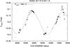 |
Fig. 1 Vmed time series for the star ASAS J011315-6411.6. A cycle with length Pcyc = 1801 d was detected by the period-search algorithms. The black line is the sinusoid best-fitting the data. |
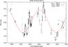 |
Fig. 2 IQR time series for the star ASAS J070153-4227.9. A cycle with length Pcyc = 1818 d (red line) was detected by the period search algorithms. A visual inspection reveals also two shorter cycles with lengths 220 and 290 d, respectively. The dark and gray lines were obtained by fitting the data with smoothing cubic splines and were plotted to highlight the cycles detected by eye. |
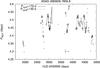 |
Fig. 3 Prot time series for the star ASAS J083656-7856.8. A visual inspection revealed two cycles with lengths 170 d and 130 d, respectively. Two smoothing cubic splines are overplotted to highlight the cycles with dark gray and light gray lines, respectively. |
In Paper I we processed the ASAS photometric time series using three different values of the sliding-window length, i.e. T = 50 d, 100 d and 150 d, producing three different time series for each activity index. The results given in Paper I have been inferred by the time series obtained with T = 50 d. As discussed there, the use of sliding-window lengths of T = 100 d and T = 150 d tends to filter out the variability phenomena occurring over a timescale shorter than 100 d, flattening the amplitude variations of the different activity indexes (see. Figs. 2–5 of Paper I). However, the activity index time series obtained with T = 100 and 150 d are more regular and smoother than those obtained with T = 50 d and are more suitable to detect long-term variations due to activity cycles. Therefore, while T = 50 d is an optimal choice for analyzing SDR as in Paper I, 100-d segments, as used here, are better suited to search for activity cycles. This difference in T obviously does not introduce any inconsistencies in, for example, correlation analysis between activity cycles and SDR.
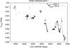 |
Fig. 4 Vmed time series for the star ASAS J082406-6334.1. The time series shows a long-term trend suggesting a cycle longer than 3000 d. A short cycle of 180 d is also visible and highlighted with a smoothing cubic spline in black. |
In Paper I, we showed that the rotation period detected in different segments slightly changes in time. This trend could be induced by the combined effect of stellar SDR and migration of Ars in latitude. Indeed, ARs placed at different latitudes rotate with different frequencies in case of SDR. The migration of ARs, due to a Schwabe-like cycle, induces a temporal variation in the detected photometric period Prot. Such a parameter can be therefore regarded as a tracer of the spot latitude migration.
This activity index has to be treated with caution. Lehtinen et al. (2016) and Lanza et al. (2016) noticed that the different rotation periods detected in different segments could also be a consequence of the ARs growth and decay occurring simultaneously at various latitudes and longitudes on the star. However, as remarked by Lehtinen et al. (2016), the use of segments with a short duration should limit this effect; see the discussion on the sliding-window length in Sect. 3.1 of Paper I and in Sect. 4.1 of Lehtinen et al. (2016) for more details. This activity index has recently been used by Vida et al. (2014) to investigate stellar cycles on Kepler data.
The Vmed index is related to the axisymmetric part of the spot distribution on the stellar surface. In fact, the higher the fractional area covered by spots evenly distributed in longitude, the lower the average photometric flux in the V band. This is one of the most used activity index to investigate activity cycles (see e.g. Rodonò et al. 2000; Messina & Guinan 2002; Lehtinen et al. 2016)
The IQR index is proportional to the stellar variability amplitude. The variability amplitude is also an index widely used to study activity cycles (see e.g. Rodonò et al. 2000; Ferreira Lopes et al. 2015; Lehtinen et al. 2016). The variability of solar-like stars is due to different phenomena acting in different timescales such as the intrinsic evolution of spots and faculae, the intrinsic evolution of ARs complexes, and flux rotational modulation induced by ARs. In this paper, the IQR index was computed in 100-daylong segments. In these intervals the main source of variability is the rotational modulation (see e.g. Messina & Guinan 2002; Lanza et al. 2003). Hence the IQR index is proportional to the amplitude of the rotational modulation signal and is related to the non-axisymmetric part of the spot distribution.
Finally, for each star we also computed a global magnetic index that is given by the average value ⟨ IQR ⟩ of the IQR time series. The ⟨ IQR ⟩ values are reported in Table 2 for all the stars investigated here.
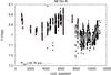 |
Fig. 5 Vmed time series for the AB Dor A. The gray squares are used to indicate the Vmed values computed in the 50-d segments. |
2.3. Computation of the global parameters for the target stars
In this paper we investigate the relationships between the cycles lengths Pcyc, activity index ⟨ IQR ⟩, and global parameters of our targets. Our analysis was focused on the following parameters: the photometric shear ΔΩphot, effective temperature Teff, convective turnover timescale τC, Rossby number Ro, radius at the bottom of the convection zone RC, dynamo number DN, and magnetic diffusivity timescale τdiff. The values ΔΩphot, Teff, τC, and Ro were computed in Paper I whereas RC, DN, and τdiff were computed in this work for the first time.
The photometric shear of a given star is defined as 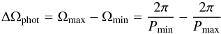 (1)where Pmin and Pmax are the minimum and maximum values of the Prot index and are interpreted as the rotation periods of two ARs occurring at two different latitudes. This parameter can be regarded as a lower limit for the SDR that is defined as
 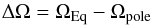 (2)where ΩEq and Ωpole are the stellar rotation frequencies at the equator and at the poles.
The effective temperature Teff and convective turnover timescale τC have been derived in Paper I using Spada et al. (2013).
The Rossby number Ro is defined as  (3)where τC is derived by the theoretical isochrones of Spada et al. (2013). Other works (Saar & Brandenburg 1999; Lehtinen et al. 2016) use the definition given by Brandenburg et al. (1998):
 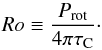 (4)In these works, the convective turnover timescale is computed through the semi-empirical equation given by Noyes et al. (1984) that expresses τC as a function of the color index B−V. In order to make a comparison between our results and those of the abovementioned works, we computed the Ro values according to the Eq. (4) and using the τC values as given by the formula of Noyes et al. (1984). In the rest of the paper, the values computed by means of Eq. (4) are indicated with the symbol RoBr, where Br stands for Brandenburg.
The dynamo number is defined as 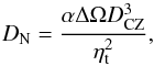 (5)with
  (6)where DCZ is the depth of the convective zone, lm is the mixing length and HD is the density scale height, ηt is the turbulent diffusivity, and ΔΩ the rotational shear. The parameters DCZ, ηt, lm, and HD occurring in Eqs. (5) and (6) were derived by the theoretical models of Spada et al. (2013). The parameter ΔΩ was replaced with the parameter ΔΩphot computed in Paper I.
Finally, the magnetic diffusivity timescale is defined as  (7)where ηt is the turbulent diffusivity; τdiff is the timescale for the turbulent dissipation of magnetic energy over a length scale DCZ. All the parameters computed for the different targets are reported in Table 2.
3. Method
We searched for activity cycles by running the Lomb-Scargle (Lomb 1976; Scargle 1982) and the phase dispersion minimization (PDM; Jurkevich 1971; Stellingwerf 1978) algorithms on the Prot, Vmed, and the IQR time series. The ASAS time series span, on average, an interval T = 3000 d. We assumed, as in Distefano et al. (2012), that a period P can be detected if P ≤ 0.75T and we performed our period search in the range (100–2000 d). We computed the False Alarm Probability (FAP) associated with a given period Pcyc according to the procedure described in Sect. 3 and we flagged a period as valid if it satisfied the requirement FAP < 0.1%. In some time series, visual inspection allowed the identification of cyclical patterns that the Lomb-Scargle and PDM algorithms were not able to detect. The failure of the period search algorithms is due to the quasi-periodic nature of the stellar cycles and to a variety of reasons: in some cases a cyclical pattern occurs only in a limited interval of the whole time series; in other cases a cyclical pattern is visible in the complete time series, but the length of the cycle changes in time. Finally, in some cases, the visual inspection suggests that the star is characterized by a cycle longer than the whole time series length. Since the size of our sample is relatively small, we decided to visually inspect each time series aiming at detecting and measuring the lengths of the cycles missed by the Lomb-Scargle and PDM algorithms. In this case, we flagged a Pcyc value as valid if at least one complete oscillation is visible (i.e., if at least two consecutive maxima or minima are clearly visible).
The uncertainty on Pcyc is estimated through the equation 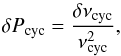 (8)where δνcyc is the uncertainty associated with the frequency of the cycle νcyc = 1 /Pcyc. This uncertainty is given by the equation:
 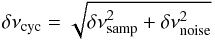 (9)where δνsamp is the uncertainty due to the limited and discrete sampling of time series and δνnoise is the uncertainty due to data noise; δνsamp and δνnoise are computed according to Kovacs (1981) through the equations
 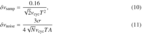 where T is the interval time spanned by the time series, σ is the standard deviation of the data before subtracting any periodic signal, N the number of time series points, and A the amplitude of the signal. In cases in which Pcyc values were determined by visual inspection we did not give a δPcyc estimate since there is not an objective way to obtain it.
False alarm probability computation
The typical Monte Carlo method used to assess the FAP of a given period P0, which has a power z0 in the Lomb-Scargle periodogram, consists in simulating N synthetic time series with the same sampling of the original time series. The synthetic data points are usually generated by means of the equation  (12)where ⟨ x ⟩ is the mean value of the original time series and R(0,σ) is a Gaussian random variate with a zero mean and a dispersion σ given by the standard deviation associated with the real data points. The Lomb-Scargle periodogram is computed for each time series and the highest peak Zmax is retained for each periodogram. The FAP associated with P0 is then computed as the fraction of synthetic time series for which Zmax ≥ z0.
The previous approach is valid only if the points of the original time series are uncorrelated, i.e., if two consecutive data points are independent of each other (see for example the discussion in Herbst & Wittenmyer 1996; Stassun et al. 1999; Rebull 2001). This is not the case for our time series, for which two consecutive elements of the activity indexes have been computed in segments that partially overlap with each other.
For this reason, we estimated the FAP by means of the Monte Carlo approach suggested by Brown et al. (1996) and also adopted by Rebull (2001) and Parihar et al. (2009). In this approach, the synthetic data points are generated by means of a recursive procedure  (13)where x0 and xi are the first element and the ith element of the simulated time series and R(0,σ) denotes a Gaussian random variate centered on zero with dispersion σ (equal to the standard deviation of the real data). The parameters α and β are defined as
  (14)where Δt = ti−ti−1 is the time interval between the two consecutive points xi−1 and xi, and Lcorr is the correlation timescale. The time series defined by Eqs. (13) is such that two points xi and xj satisfy the property
  (15)where C2(i,j) is the two-points correlation function and Δtij = ti−tj the time between xi and xj (Brown et al. 1996). In our case, we adopted Lcorr = T/ 3 were T is the length of the sliding window used to generate the activity index time series.
In order to assess the FAP probability associated with the period detected in a given time series we followed the Monte Carlo procedure described above by generating 10 000 synthetic time series. If the period was found by means of the Lomb-Scargle algorithm, the FAP was computed by taking the fraction of synthetic time series for which Zmax>z0. If the period P0 was found by means of the PDM algorithm, we ran the PDM on each synthetic time series and we retained the minimum value θmin of the PDM periodogram for each time series. The FAP was then computed by taking the fraction of the synthetic time series for which θ0<θmin, where θ0 is the PDM estimator associated with P0.
4. Results
4.1. Results of time series analysis
We detected activity cycles in 67 stars. We found two distinct cycles in 32 of the stars and more than two cycles in 16 stars. The results of our analysis are reported in Table 3. In this table we listed the Pcyc lengths found for each star. For each cycle we reported a flag indicating the activity index from which Pcyc was inferred and a second flag indicating the method used to detect the period. If Pcyc was inferred by means of the Lomb-Scargle or the PDM algorithm, we also reported the associated FAP.
In Figs. 1–4 we report some examples of our analysis. In Fig. 1 we show the Vmed time series for the star ASAS J011315-6411.6. The period search algorithms detected in this case a cycle with Pcyc = 1801 d. The sinusoid best fitting the data is overplotted (red continuous line).
In Fig. 2 we plot the IQR time series for the star ASAS J070153-4227.9. The Lomb-Scargle periodgram of this time series gives a highly significant peak at P = 1818 d. However, visual inspection also reveals the two shortest cycles with lengths of 220 and 290 d, respectively. These cycles could be secondary cycles analoguous to the Rieger cycles or to the quasi-biennal oscillations superimposed on the 11-yr solar cycle.
In Fig. 3 we report the Prot time series for the star ASAS 083656-7856.8. The Lomb-Scargle and PDM algorithms were not able to detect any significant period in this star. However two cycles with lengths 170 d and 130 d are clearly visible in the data. These features are very common in the Sun and in solar-like stars. For instance, the Rieger cycles and the quasi-biennal oscillations have been well detected in the Sun but, as remarked by Oláh et al. (2016), they are not continuously present in the solar data registered until now. Oláh et al. (2016) noticed in the Mount Wilson time series that some of the detected cycles are only temporarily seen and that young stars are characterized by cycles whose duration changes in time. Rieger-like cycles were also detected by Lanza et al. (2009) in CoRoT-2 and by Bonomo & Lanza (2012) in Kepler-17.
Finally in Fig. 4, we report the Vmed time series of the star ASAS J082406-6334.1. The visual inspection suggests the existence of a cycle longer than 3000 d. A shorter cycle with Pcyc = 180 d is also detected by eye and is highlighted with the black continuous line. Some of the Pcyc values detected by visual inspection are shorter than the sliding-window length used to process the ASAS time series. In fact, the 100-d sliding window attenuates the periodic signals shorter than 100 d but, in some cases, does not completely suppress them. So if these signal have a sufficient amplitude, they can still be detected after the segmentation procedure (see Appendix A for details).
4.2. Case of AB Dor A
To the best of our knowledge, the cycles reported in Table 3 have been detected here for the first time. The only exception in our sample is given by AB Dor A (HD 36705) which is identified with the ASAS ID J052845-6526.9. AB Dor A is a fast rotating (Prot = 0.51 d) K1V star that is well studied in the literature and is the primary component of the quadruple system AB Dor, which also comprises the stars AB Dor Ba, AB Dor Bb, and AB Dor C. AB Dor Ba and AB Dor Bb are the components of the binary system AB Dor B, which was resolved for the first time by Janson et al. (2007) and is located at 8.9′′ ± 0.1′′ from AB Dor A (Martin & Brandner 1995). AB Dor C is a close companion of AB Dor A. It was detected by Guirado et al. (1997) and it is located at about 0.16′′ from AB Dor A. Guirado et al. (2010) made a dynamical estimate of the AB Dor A mass and obtained M = 0.86 ± 0.09 M⊙, which is in good agreement with the photometric estimate M = 0.93 M⊙ made in Paper I and based on the theoretical isochrones of Spada et al. (2013; see Paper I for details).
The magnetic activity of AB Dor A has been widely studied in the literature by means of spectroscopic and photometric data collected at different wavelengths (see e.g. Drake et al. 2015; Lalitha & Schmitt 2013; Budding et al. 2009; Lalitha & Schmitt 2013; Jeffers et al. 2007; Messina et al. 2006; Järvinen et al. 2005, and references therein)
Järvinen et al. (2005) merged the photometric data collected in several works and obtained a V-band time-serie spanning 1978–2000. These authors analyzed these data with the inversion technique developed by Berdyugina (1998) to study the temporal evolution of the spots longitude distribution. They analyzed the temporal variations of the spots longitudes and mean brightness by means of a Fourier analysis and detected a primary cycle with length Pcyc1 = 21 ± 3 yr and a secondary cycle with length Pcyc2 ~ 5.5 yr. The primary cycle is mainly associated with the mean magnitude variations, while the secondary cycle is a flip-flop cycle, i.e., a periodic switch of the longitude where the dominant spot concentration occurs. Järvinen et al. (2005) remarked that their estimate of the primary cycle length is not very accurate because of the sparseness of data in the years 1978–1985. We merged the photometric data reported in literature and summarized in Järvinen et al. (2005) with the ASAS data and we obtained a 27-yr V-band time series. We processed this longterm dataset with the sliding window algorithm described in Paper I and we obtained three 27-yr time series for the activity indexes Vmed, Prot, and IQR. In this specific case, we used a 50-d sliding window because the duration of the different observing seasons usually do not exceed two months and therefore, the use of a 100-d sliding window should be meaningless. The analysis of the Vmed time series with the Lomb-Scargle algorithm revealed an activity cycle of length Pcyc = 16.78 ± 2 yr. In Fig. 5 we plot the long-term photometric time series and the sinusoid that best fits the data.
The use of the activity indexes time series also allowed the detection of secondary cycles with lengths of 400 d, 190 d, and 90 d, respectively.
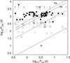 |
Fig. 6 Pcyc length versus stellar rotation period Prot. The filled circles indicate the primary cycles and the empty circles the secondary cycles. The arrows indicate the stars for which the visual inspection of time series revealed Pcyc ≥ 3000 d. The continuous line, dashed line, and dotted line represent the Aa, Ab, and I sequences identified by Böhm-Vitense (2007), respectively. The dash-dotted line represents the locus where the |
5. Discussion
5.1. Relationships between cycle length, rotation period and Rossby number
Since stellar activity cycles were first detected, a relationship has been searched between the cycle period Pcyc and t stellar rotation period Prot. Böhm-Vitense (2007) analyzed a sample of stars obtained by selecting the best quality spectrophotometric data collected at Mt. Wilson. She identified three different stellar sequences that have an almost constant ratio . The Aa and Ab sequences (where A stands for active) consist of young and active stars. The ratio is between 400 and 500 for the Aa stars and is about 300 for the Ab stars. The I sequence (where I stands for inactive) comprises old and less active stars for which the ratio is about 90. Böhm-Vitense (2007) speculates that the three sequences are due to different kind of dynamos excited by different phenomena. According to her interpretation, the dynamo should be generated by SDR in A sequence stars and by a vertical shear in I sequence stars.
In Fig. 6 we plot the cycle lengths versus stellar rotation periods as in Böhm-Vitense (2007). The filled circles indicate the primary cycles and the empty circles indicate the secondary cycles. We also overplotted the three sequences identified by Böhm-Vitense (2007) and a fourth line corresponding to the Pcyc/Prot ≃ 5 ratio of the solar Rieger cycle. The figure shows that the primary cycles do not follow any particular trend and that their lengths seem to be uncorrelated with the rotation periods. The secondary cycles are also uniformly distributed between the Ab and I sequences and do not follow any particular pattern. Some of the secondary cycles lie beneath the I sequence and their Pcyc/Prot ratio is very close to that of the solar Rieger-cycle.
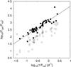 |
Fig. 7
|
Other authors (see e.g. Baliunas et al. 1996; Vida et al. 2014; Oláh et al. 2016) searched for a correlation between and the parameter  that, according to Baliunas et al. (1996), should be proportional to the dynamo number D. In these works a linear fit is performed investigating the relationship between the logarithms of the two quantities. The slope m extracted from the linear fit is the exponent of the power law Pcyc/Prot = (1 /Prot)m. If m is close to 1 then no correlation exists between Pcyc and Prot. Baliunas et al. (1996) found m = 0.74, which is in agreement with the value m = 0.76 recently found by Oláh et al. (2016).
In Fig. 7 we plotted  versus
  for our targets. We performed a linear fit between the two quantities and we found m = 1.02 ± 0.06 that indicates no correlation between Pcyc and Prot. Our results are slightly higher than those found by Baliunas et al. (1996) and Oláh et al. (2016) but are in close agreement with those found by Savanov (2012) and Lehtinen et al. (2016).
The lack of correlation between Pcyc and Prot seen in Fig. 6 and in Fig. 7 suggests that the dynamo mechanism occurring in our young targets stars is different from that acting in the older Mt. Wilson stars selected by Böhm-Vitense (2007).
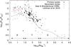 |
Fig. 8 Ratio of |
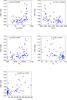 |
Fig. 9 ⟨ IQR ⟩ versus parameters τdiff, Teff, DN, RC, and τC, respectively. In each panel the Spearman coefficient rS and the corresponding two-sided p-value are shown. |
The lack of correlation between Pcyc and Prot seen in our targets could be related to their low Rossby number values. In fact, most of our targets are fast rotating stars (Prot< 10 d) with Ro values falling in the range (0.004–0.17) and RoBr values in the range (0.002–0.06). These ranges are very different from those covered by the Mt. Wilson stars. Saar & Brandenburg (1999) extended the sample of the Mt. Wilson stars with an ensemble of young and fast rotating stars and showed that these stars formed a third branch in the ( ,
,  ) plane. This branch was called the super active branch and was clearly distinct from the active and inactive branches and was attributed to a different dynamo mechanism. Recently, Lehtinen et al. (2016) exploited long-term photometry to measure the cycle length Pcyc of 21 young active stars and found that the active and the super active branch are connected by a transitional branch. In Fig. 8 we plotted the values versus the values inferred for our stars. In the plot we also reported the data from Saar & Brandenburg (1999) and from Lehtinen et al. (2016). The primary cycles of our stars are in good agreement with the transitional branch as defined by Lehtinen et al. (2016). Also Lehtinen et al. (2016) did not find any correlation between Pcyc and Prot in their targets. Hence, we can conclude that in stars belonging to the transitional branch, the cycle length Pcyc and the rotation period Prot are uncorrelated.
5.2. Relationship between Pcyc and global stellar parameters
We investigated how the cycle lengths Pcyc are related to the global stellar parameters of our targets. We evaluated the degree of the correlation between Pcyc and a given parameter by computing the Spearman rank-order correlation coefficient (rS) (Press et al. 1992). This coefficient is a nonparametric measure of the monotonicity of the relationship between two datasets.
A value of rS close to 0 implies that the two datasets are poorly correlated, whereas the closer rS is to ±1 the stronger the monotonic relationship between the two variables.
The statistical significance of a given value rS = r0 can be evaluated by computing the two-sided p-value, i.e., the probability (P( | rS | ≥ | r0 |) under the null hypothesys that two invesigated datasets are non-monotonically correlated (Press et al. 1992).
In Table 2 we reported the Spearman correlation coefficients between the length Pcyc of the primary cycles and the various stellar parameters. The corresponding p-values are also reported. The values of | rS | are very close to 0 in all the cases indicating a poor correlation between Pcyc and the different variables.
5.3. Relationship between ⟨ IQR ⟩ and global stellar parameters
As remarked in Sect. 2, the IQR index is proportional to the amplitude of the rotational modulation signature and is related to the non-axisymmetric part of the spot distribution. The amplitude of rotational modulation is a widely used activity index and can be regarded as a robust proxy of the surface magnetic activity. García et al. (2013) demonstrated that the variance of the TSI, computed on a 60-d sliding window, closely mimics the variations of the 10.7 cm radio flux that in turn is a good indicator of the solar magnetic activity (see Bruevich et al. 2014, for details). We computed the Spearman coefficient between ⟨ IQR ⟩ and different stellar parameters to investigate how the mean level of the stellar surface magnetic activity is linked to the stellar properties. In Table 3 we reported the values of rS for the different parameters. In this case, rS values are significantly higher then those computed for Pcyc. A good correlation (| rS | ≃ 0.5) is seen between ⟨ IQR ⟩ and Teff, τC, τdiff, RC and DN. The sign of correlation is positive for τC, τdiff and DN and negative for Teff and RC.
In Fig. 9 we reported ⟨ IQR ⟩ versus the various stellar parameters for which a significant correlation is seen (rS ≃ 0.5). Despite the scatter in the data, the different plots clearly show that ⟨ IQR ⟩ tends to increase with τdiff, τC, and Teff and has a negative correlation with Teff and RC.
Spearman correlation coefficient between Pcyc and different stellar parameters.
Spearman correlation coefficient rS between ⟨ IQR ⟩ and different stellar parameters.
A weaker but still significant correlation is also seen between ⟨ IQR ⟩ and the photometric shear ΔΩphot. In Fig. 10 we plotted ⟨ IQR ⟩ versus ΔΩphot. The various stars are color-coded according to their effective temperature Teff. The plot shows that
-
ΔΩphottends to increase with temperature (as demonstrated in Paper I);
-
the sign of the correlation between ⟨ IQR ⟩ and ΔΩphot and ⟨ IQR ⟩ is negative (rS = −0.43). This means that the lower ΔΩphot the higher ⟨ IQR ⟩.
These results are in very good agreement with the theoretical models developed by Kitchatinov & Olemskoy (2011). In fact, these models predict that even a small SDR is very efficient for dynamos in M-type stars, it is less efficient in K and G type and even a strong SDR is inefficient in F-type stars.
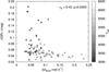 |
Fig. 10 ⟨ IQR ⟩ versus ΔΩphot. The points are color coded according the stellar effective temperature Teff. |
5.4. Evolution of Pcyc and ⟨ IQR ⟩ with the stellar age
Oláh et al. (2016) investigated how the  ratio depends on the stellar age. They found that exhibits a large scatter in the younger and more active stars of their sample whereas the older stars have about the same value. The age at which becomes constant is, according to their work, at about 2.2 Gyr, i.e., the age of the Vaughan-Preston gap (Vaughan & Preston 1980). The sample of stars analyzed by Oláh et al. (2016) covers the age range 200–6200 Myr. Our work permits us to extend the age range studied by Oláh et al. (2016) and to investigate the transition age between the pre-main sequence (PMS) and the main sequence (MS) phase. Our analysis is slightly different from that performed by Oláh et al. (2016). We decided to investigate the relationship between Pcyc and the stellar age instead of the relationship between and the stellar age. In fact, the trend of the between ratio, in the age range covered by our targets, could be dominated by the complex Prot evolution seen in the PMS stars (see e.g. Lanzafame & Spada 2015, and references therein). In the top panel of Fig. 11, we reported the length of the primary cycles Pcyc versus the stellar age. The blue filled symbols indicate the cycles identified in the present work and the red empty symbols mark those found by Oláh et al. (2016). The picture shows that Pcyc is about constant in the age range 4−300 Myr. After 300 Myr, the cycle lengths are more scattered and seem to increase with the stellar age. After 2.2 Gyr, that is the age corresponding to the Vaughan-Preston gap, the scatter in Pcyc decreases as described by Oláh et al. (2016). Although our data cover an interval of about 3000 d, which could prevent the detection of longer cycles, we observed long-term trends suggesting cycles longer than 3000 d in just 11 of the 90 investigated targets. For this reason, we are confident that our data are not seriously affected by a selection bias and that the age range investigated here is really, on average, characterized by cycles shorter than those observed in the older Mt. Wilson stars. In the bottom panel of Fig. 11 we plotted ⟨ IQR ⟩ versus the stellar age. The picture shows that ⟨ IQR ⟩ tends to decrease with the stellar age as also indicated by the Spearman coefficient rS = 0.39. This result is in agreement with all the works that studied the evolution of the level of magnetic activity versus age (see e.g. Žerjal et al. 2017; Oláh et al. 2016, and references therein)
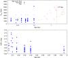 |
Fig. 11 Top panel: Pcyc versus the stellar age. The blue filled circles refer to the primary cycles detected in the present work and the red empty circles to the data reported by Oláh et al. (2016). The blue arrows indicate the stars for which the visual inspection of time series revealed Pcyc ≥ 3000 d. Bottom panel: activity index ⟨ IQR ⟩ versus the stellar age is shown. |
5.5. Butterfly diagrams
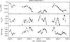 |
Fig. 12 Time series for star ASAS J070030-7941.8. Top panel: Vmed time series for the star ASAS J070030-7941.8 is shown. Middle panel: Prot time series is shown. Bottom panel: IQR time series is shown. A primary cycle with length Pcyc = 1834 d was detected in the Vmed time series and the sinusoid best fitting the data was overplotted on it (red dashed line). The Prot and the IQR time series exhibit cycles (dark continuous lines) shorter than the primary cycle. The black dotted lines indicate the times at which maxima occur in the Prot time series. |
In the Sun, the latitudes at which ARs occur change versus time according to the so-called “butterfly-diagram”. At the beginning of a solar cycle, ARs emerge in belts located at intermediate latitudes (± 35deg). As the cycle progresses, the ARs formation regions migrate toward the equator. At the beginning of the next cycle, the ARs form again at intermediate latitudes. The solar SDR combined with the ARs migration determines a decrease in the rotation period detectable along the 11-yr cycle because the ARs located at intermediate latitudes rotate more slowly than those located at the equator. As remarked in Paper I and in Sect. 2.2, the activity index Prot of a given star can therefore be regarded as a tracer of the ARs migration in latitude. This activity index cannot give information about the exact latitudes at which ARs occur but can give insight into the nature of stellar magnetic field. In fact, in a star with a solar-like dynamo, we expect that the trend of Prot with time mimics that of the solar butterfly diagram, i.e., that during a given cycle Prot decreases in time and that it rises rapidly to higher values at the beginning of the next cycle. Messina & Guinan (2003), for instance, analyzed the trend of Prot in six young solar analogues. They noticed that three of these stars follow a solar behavior whereas the other three show an anti-solar behaviour with Prot increasing during the cycle. The Prot time series of our target stars, in general, have fewer points than the Vmed and IQR time series. Indeed, as remarked in Paper I, Prot is detectable in a given time interval only if ARs maintain a stable configuration. In Figs. 12 and 13 we reported the Prot time series for the stars ASAS J070030-7941.8 and ASAS J055329-8156.9 which are the targets with the highest number of Prot determinations. The Vmed time series and IQR time series of the two stars are also reported for comparison. The stars have two primary cycles with length Pcyc = 1834 d and Pcyc = 1290 d, respectively. The two sinusoids that best fit the data and correspond to the primary cycles are overplotted on the Vmed time series. The visual inspection of the pictures shows that in both stars:
-
the Prot index oscillates with a cycle shorter than the primary cycle;hence the ARs latitude migration occurs in a timescale shorterthan the length of the primary cycle;
-
in some intervals, the trend of Prot vs time mimics the trends of Vmed and IQR and the maxima and minima of Prot correspond to local maxima and minima of the Vmed and IQR time series; in other intervals the maxima and minima of Prot are uncorrelated with those of the Vmed and IQR time series. This implies that in some time intervals the changes in AR latitudes are correlated with the variations in the ARs areas and in the mean level of magnetic activity whereas in some other intervals there is no correlation;
-
the Prot variations with time are very different from those occurring in the Sun. Rise patterns are followed by decreasing patterns. This implies that ARs first migrate from regions with shorter rotation periods to regions with higher rotation periods and then migrate in the opposite sense. In the Sun the migration occurs in only one sense i.e. from the intermediate latitudes to the equator.
Similar trends are observed in all the targets analyzed here.
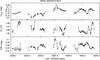 |
Fig. 13 Time series for star ASAS J055329-8156.9. Top panel: the Vmed time series for the star ASAS J055329-8156.9 is shown. Middle panel: the Prot time series is shown. Bottom panel: the IQR time series is shown. A primary cycle with length Pcyc = 1290 d was detected in the Vmed time series and the sinusoid best fitting the data was overplotted on it (red dashed line). The Prot and IQR time series exhibit cycles (dark continuous lines) shorter than the primary cycle. The black dotted lines indicate the times at which maxima and minima occur in the Prot time series. |
The patterns seen in the Prot time series of our targets can be regarded as a further evidence that the dynamo acting in these stars is very different from that acting in the Sun.
6. Conclusions
In the present work we searched for activity cycles in stars belonging to young loose stellar associations covering the age range 4−95 Myr. We investigated the correlation between cycle properties and global stellar parameters and how cycle properties evolve with the stellar age. In particular, our work extends the age range covered by the Mt Wilson stars whose properties have recently been reanalyzed by Oláh et al. (2016).
We analyzed the long-term time series of three different activity indexes and we were able to detect activity cycles in 67 stars and to measure their length Pcyc. About half of these stars show multiple and complex cycles according to the results found by Oláh et al. (2016) for young and active stars. Some of the detected secondary cycles have a ratio similar to that of the solar Rieger-cycles  .
.
We investigated how Pcyc is correlated with the photometric shear ΔΩphot, effective temperature Teff, convective turnover timescale τC, Rossby number Ro, radius at the bottom of the convection zone RC, dynamo number DN, and magnetic diffusivity timescale τdiff. We found that Pcyc is essentially uncorrelated with the abovementioned parameters in our targets. The lack of correlation between Pcyc and Prot suggests that the dynamo acting in our targets is different from that acting in the active and inactive branches determined by Böhm-Vitense (2007). Indeed, the location of our targets in the  plane is in good agreement with the transitional branch as determined by Lehtinen et al. (2016). The activity index ⟨ IQR ⟩, which can be regarded as a proxy of the magnetic surface activity level, is positively correlated with τC, τdiff, DN and negatively correlated with Teff and RC. The analysis of the relationship between ⟨ IQR ⟩, SDR, and Teff supports the theoretical models developed by Kitchatinov & Olemskoy (2011). Indeed, in agreement with these models, even a small differential rotation is efficient for dynamos in M-type stars, but it becomes less efficient or completely inefficient at increasing Teff (cf. Fig. 10).
The analysis of the butterfly diagrams of our target stars shows two main features. The first is that the ARs migration in latitude occurs over a timescale shorter than the primary cycle; the second is that the latitudes at which ARs emerge seem to oscillate from a maximum to a minimum latitude and vice-versa. This is very different from the solar behaviour where the spots migrate only from intermediate latitudes to the equator. We merged our data with those analyzed by Oláh et al. (2016) and we studied how Pcyc evolve with the stellar age. We found that Pcyc is about constant and does not show significant correlation with the stellar age in the range (4−300 Myr); after 300 Myr Pcyc values are quite scattered and tend to increase with the stellar age; and after 2.2 Gyr, Pcyc values tend to be less scattered and seem to converge to the solar value as described by Oláh et al. (2016). The activity index ⟨ IQR ⟩ decreases with the stellar age in the age range 4–95 Myr. Finally, we merged the ASAS time series of the star AB Dor A with the photometric data from previous works and we detected a cycle with length Pcyc = 16.78 ± 2 yr and shorter secondary cycles with lengths of 400 d, 190 d, and 90 d.
Acknowledgments
The authors are grateful to the referee Lauri Jetsu for helpful comments and suggestions.
References
- Baliunas, S. L., & Vaughan, A. H. 1985, ARA&A, 23, 379 [NASA ADS] [CrossRef] [Google Scholar]
- Baliunas, S. L., Donahue, R. A., Soon, W. H., et al. 1995, ApJ, 438, 269 [NASA ADS] [CrossRef] [Google Scholar]
- Baliunas, S. L., Nesme-Ribes, E., Sokoloff, D., & Soon, W. H. 1996, ApJ, 460, 848 [NASA ADS] [CrossRef] [Google Scholar]
- Ballester, J. L., Oliver, R., & Carbonell, M. 2002, ApJ, 566, 505 [NASA ADS] [CrossRef] [Google Scholar]
- Berdyugina, S. V. 1998, A&A, 338, 97 [NASA ADS] [Google Scholar]
- Böhm-Vitense, E. 2007, ApJ, 657, 486 [NASA ADS] [CrossRef] [Google Scholar]
- Bonomo, A. S., & Lanza, A. F. 2012, A&A, 547, A37 [NASA ADS] [CrossRef] [EDP Sciences] [Google Scholar]
- Brandenburg, A., Saar, S. H., & Turpin, C. R. 1998, ApJ, 498, L51 [NASA ADS] [CrossRef] [Google Scholar]
- Brown, A., Deeney, B. D., Ayres, T. R., Veale, A., & Bennett, P. D. 1996, ApJS, 107, 263 [NASA ADS] [CrossRef] [Google Scholar]
- Bruevich, E. A., Bruevich, V. V., & Yakunina, G. V. 2014, JA&A, 35, 1 [NASA ADS] [Google Scholar]
- Budding, E., Erdem, A., Innis, J. L., Oláh, K., & Slee, O. B. 2009, Astron. Nachr., 330, 358 [NASA ADS] [CrossRef] [Google Scholar]
- Butters, O. W., West, R. G., Anderson, D. R., et al. 2010, A&A, 520, L10 [NASA ADS] [CrossRef] [EDP Sciences] [Google Scholar]
- Distefano, E., Lanzafame, A. C., Lanza, A. F., et al. 2012, MNRAS, 421, 2774 [NASA ADS] [CrossRef] [MathSciNet] [Google Scholar]
- Distefano, E., Lanzafame, A. C., Lanza, A. F., Messina, S., & Spada, F. 2016, A&A, 591, A43 [NASA ADS] [CrossRef] [EDP Sciences] [Google Scholar]
- Drake, J. J., Chung, S. M., Kashyap, V. L., & Garcia-Alvarez, D. 2015, ApJ, 802, 62 [NASA ADS] [CrossRef] [Google Scholar]
- Durney, B. R., Mihalas, D., & Robinson, R. D. 1981, PASP, 93, 537 [NASA ADS] [CrossRef] [Google Scholar]
- Ferreira Lopes, C. E., Leão, I. C., de Freitas, D. B., et al. 2015, A&A, 583, A134 [NASA ADS] [CrossRef] [EDP Sciences] [Google Scholar]
- García, R. A., Salabert, D., Mathur, S., et al. 2013, in J. Phys. Conf. Ser., 440, 012020 [NASA ADS] [CrossRef] [Google Scholar]
- García, R. A., Ceillier, T., Salabert, D., et al. 2014, A&A, 572, A34 [NASA ADS] [CrossRef] [EDP Sciences] [Google Scholar]
- Gleissberg, W. 1958, Z. Astrophys., 46, 219 [NASA ADS] [Google Scholar]
- Gnevyshev, M. N. 1967, Sol. Phys., 1, 107 [NASA ADS] [CrossRef] [Google Scholar]
- Gnevyshev, M. N. 1977, Sol. Phys., 51, 175 [NASA ADS] [CrossRef] [Google Scholar]
- Guirado, J. C., Reynolds, J. E., Lestrade, J.-F., et al. 1997, ApJ, 490, 835 [NASA ADS] [CrossRef] [Google Scholar]
- Guirado, J. C., Martí-Vidal, I., Marcaide, J. M., et al. 2010, Astrophys. Space Sci. Proc., 14, 139 [NASA ADS] [CrossRef] [Google Scholar]
- Hale, G. E., Ellerman, F., Nicholson, S. B., & Joy, A. H. 1919, ApJ, 49, 153 [NASA ADS] [CrossRef] [Google Scholar]
- Hathaway, D. H. 2015, Liv. Rev. Sol. Phys., 12, 4 [Google Scholar]
- Herbst, W., & Wittenmyer, R. 1996, in BASS, 28, 1338 [Google Scholar]
- Janson, M., Brandner, W., Lenzen, R., et al. 2007, A&A, 462, 615 [NASA ADS] [CrossRef] [EDP Sciences] [Google Scholar]
- Järvinen, S. P., Berdyugina, S. V., Tuominen, I., Cutispoto, G., & Bos, M. 2005, A&A, 432, 657 [NASA ADS] [CrossRef] [EDP Sciences] [Google Scholar]
- Jeffers, S. V., Donati, J.-F., & Collier Cameron, A. 2007, MNRAS, 375, 567 [NASA ADS] [CrossRef] [Google Scholar]
- Jurkevich, I. 1971, Ap&SS, 13, 154 [NASA ADS] [CrossRef] [Google Scholar]
- Kitchatinov, L. L., & Olemskoy, S. V. 2011, MNRAS, 411, 1059 [NASA ADS] [CrossRef] [Google Scholar]
- Kovacs, G. 1981, Ap&SS, 78, 175 [NASA ADS] [CrossRef] [EDP Sciences] [Google Scholar]
- Lalitha, S., & Schmitt, J. H. M. M. 2013, A&A, 559, A119 [NASA ADS] [CrossRef] [EDP Sciences] [Google Scholar]
- Lanza, A. F., Rodonò, M., Pagano, I., Barge, P., & Lebaria, A. 2003, A&A, 403, 1135 [NASA ADS] [CrossRef] [EDP Sciences] [Google Scholar]
- Lanza, A. F., Pagano, I., Leto, G., et al. 2009, A&A, 493, 193 [NASA ADS] [CrossRef] [EDP Sciences] [Google Scholar]
- Lanza, A. F., Flaccomio, E., Messina, S., et al. 2016, A&A, 592, A140 [NASA ADS] [CrossRef] [EDP Sciences] [Google Scholar]
- Lanzafame, A. C., & Spada, F. 2015, A&A, 584, A30 [NASA ADS] [CrossRef] [EDP Sciences] [Google Scholar]
- Lean, J. 1990, ApJ, 363, 718 [NASA ADS] [CrossRef] [Google Scholar]
- Lehtinen, J., Jetsu, L., Hackman, T., Kajatkari, P., & Henry, G. W. 2016, A&A, 588, A38 [NASA ADS] [CrossRef] [EDP Sciences] [Google Scholar]
- Lomb, N. R. 1976, Ap&SS, 39, 447 [NASA ADS] [CrossRef] [Google Scholar]
- Martin, E. L., & Brandner, W. 1995, A&A, 294, 744 [NASA ADS] [Google Scholar]
- Messina, S., & Guinan, E. F. 2002, A&A, 393, 225 [NASA ADS] [CrossRef] [EDP Sciences] [Google Scholar]
- Messina, S., & Guinan, E. F. 2003, A&A, 409, 1017 [NASA ADS] [CrossRef] [EDP Sciences] [Google Scholar]
- Messina, S., Cutispoto, G., Guinan, E. F., Lanza, A. F., & Rodonò, M. 2006, A&A, 447, 293 [NASA ADS] [CrossRef] [EDP Sciences] [Google Scholar]
- Noyes, R. W., Hartmann, L. W., Baliunas, S. L., Duncan, D. K., & Vaughan, A. H. 1984, ApJ, 279, 763 [NASA ADS] [CrossRef] [Google Scholar]
- Oláh, K., Kolláth, Z., Granzer, T., et al. 2009, A&A, 501, 703 [NASA ADS] [CrossRef] [EDP Sciences] [Google Scholar]
- Oláh, K., Kővári, Z., Petrovay, K., et al. 2016, A&A, 590, A133 [NASA ADS] [CrossRef] [EDP Sciences] [Google Scholar]
- Oliver, R., Ballester, J. L., & Baudin, F. 1998, Nature, 394, 552 [NASA ADS] [CrossRef] [Google Scholar]
- Parihar, P., Messina, S., Distefano, E., Shantikumar, N. S., & Medhi, B. J. 2009, MNRAS, 400, 603 [NASA ADS] [CrossRef] [Google Scholar]
- Pojmanski, G. 1997, Acta Astron., 47, 467 [NASA ADS] [Google Scholar]
- Press, W. H., Teukolsky, S. A., Vetterling, W. T., & Flannery, B. P. 1992, Numerical recipes in C., The art of scientific computing [Google Scholar]
- Rebull, L. M. 2001, AJ, 121, 1676 [NASA ADS] [CrossRef] [Google Scholar]
- Rieger, E., Kanbach, G., Reppin, C., et al. 1984, Nature, 312, 623 [NASA ADS] [CrossRef] [Google Scholar]
- Rodonò, M., Messina, S., Lanza, A. F., Cutispoto, G., & Teriaca, L. 2000, A&A, 358, 624 [NASA ADS] [Google Scholar]
- Saar, S. H., & Brandenburg, A. 1999, ApJ, 524, 295 [NASA ADS] [CrossRef] [Google Scholar]
- Savanov, I. S. 2012, Astron. Rep., 56, 716 [NASA ADS] [CrossRef] [Google Scholar]
- Scargle, J. D. 1982, ApJ, 263, 835 [NASA ADS] [CrossRef] [Google Scholar]
- See, V., Jardine, M., Vidotto, A. A., et al. 2016, MNRAS, 462, 4442 [NASA ADS] [CrossRef] [Google Scholar]
- Soon, W. H., Baliunas, S. L., & Zhang, Q. 1993, ApJ, 414, L33 [NASA ADS] [CrossRef] [Google Scholar]
- Spada, F., Demarque, P., Kim, Y.-C., & Sills, A. 2013, ApJ, 776, 87 [NASA ADS] [CrossRef] [Google Scholar]
- Stassun, K. G., Mathieu, R. D., Mazeh, T., & Vrba, F. J. 1999, AJ, 117, 2941 [NASA ADS] [CrossRef] [Google Scholar]
- Stellingwerf, R. F. 1978, ApJ, 224, 953 [NASA ADS] [CrossRef] [Google Scholar]
- Suárez Mascareño, A., Rebolo, R., & González Hernández, J. I. 2016, A&A, 595, A12 [NASA ADS] [CrossRef] [EDP Sciences] [Google Scholar]
- Žerjal, M., Zwitter, T., Matijevič, G., et al. 2017, ApJ, 835, 61 [NASA ADS] [CrossRef] [Google Scholar]
- Vaughan, A. H., & Preston, G. W. 1980, PASP, 92, 385 [NASA ADS] [CrossRef] [Google Scholar]
- Vida, K., Oláh, K., & Szabó, R. 2014, MNRAS, 441, 2744 [NASA ADS] [CrossRef] [Google Scholar]
- Wilson, O. C. 1978, ApJ, 226, 379 [NASA ADS] [CrossRef] [Google Scholar]
Appendix A: Effect of the sliding-window algorithm on a periodic signal
The segmentation procedure used to derive activity indexes is equivalent to a low-pass filter. This preserves the signals with a frequency lower than a certain cutoff frequency and attenuates signals with frequencies higher than the cutoff frequency. In our case, the use of a sliding-window with length T = 100 d attenuates signals with periods shorter than 100-d but, in some cases, does not completely suppress them. We performed different tests by simulating sinusoidal signals with different amplitudes and periods and by processing them with our segmentation algorithm. In the top panel of Fig. A.1 we plotted a simulated time series obtained by combining two sinusoidal signals with periods P1 = 300 d, P2 = 45 d and amplitudes A1 = 0.4, A2 = 0.6, respectively. A white gaussian noise with variance σ = 0.1 was added to the simulated data. In the bottom panel, we plotted the filtered signal obtained after processing the simulated time series with our segmentation algorithm. The filter has attenuated but not suppressed the 45-d signal. In Fig. A.2 we reported a similar test obtained by combining two period signals P1 = 300 d, P2 = 45 d and amplitudes A1 = 0.4, A2 = 0.1. In this second case the signal with P = 45 d is completely suppressed.
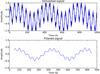 |
Fig. A.1 Top panel: a simulated time series obtained by combining two sinusoidal signals with periods P1 = 300 d, P2 = 45 d and amplitudes A1 = 0.4, A2 = 0.6, respectively. Bottom panel: filtered time series. The segmentation algorithm attenuates but does not suppress the signal with P = 45 d. |
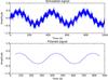 |
Fig. A.2 Top panel: a simulated time series obtained by combining two period signals with periods P1 = 300 d, P2 = 45 d and amplitudes A1 = 0.4, A2 = 0.1, respectively. Bottom panel: filtered time series. The 45-d is completely suppressed in this case. |
All Tables
Spearman correlation coefficient rS between ⟨ IQR ⟩ and different stellar parameters.
All Figures
|
Fig. 1 Vmed time series for the star ASAS J011315-6411.6. A cycle with length Pcyc = 1801 d was detected by the period-search algorithms. The black line is the sinusoid best-fitting the data. |
| In the text | |
|
Fig. 2 IQR time series for the star ASAS J070153-4227.9. A cycle with length Pcyc = 1818 d (red line) was detected by the period search algorithms. A visual inspection reveals also two shorter cycles with lengths 220 and 290 d, respectively. The dark and gray lines were obtained by fitting the data with smoothing cubic splines and were plotted to highlight the cycles detected by eye. |
| In the text | |
|
Fig. 3 Prot time series for the star ASAS J083656-7856.8. A visual inspection revealed two cycles with lengths 170 d and 130 d, respectively. Two smoothing cubic splines are overplotted to highlight the cycles with dark gray and light gray lines, respectively. |
| In the text | |
|
Fig. 4 Vmed time series for the star ASAS J082406-6334.1. The time series shows a long-term trend suggesting a cycle longer than 3000 d. A short cycle of 180 d is also visible and highlighted with a smoothing cubic spline in black. |
| In the text | |
|
Fig. 5 Vmed time series for the AB Dor A. The gray squares are used to indicate the Vmed values computed in the 50-d segments. |
| In the text | |
|
Fig. 6 Pcyc length versus stellar rotation period Prot. The filled circles indicate the primary cycles and the empty circles the secondary cycles. The arrows indicate the stars for which the visual inspection of time series revealed Pcyc ≥ 3000 d. The continuous line, dashed line, and dotted line represent the Aa, Ab, and I sequences identified by Böhm-Vitense (2007), respectively. The dash-dotted line represents the locus where the |
| In the text | |
|
Fig. 7
|
| In the text | |
|
Fig. 8 Ratio of |
| In the text | |
|
Fig. 9 ⟨ IQR ⟩ versus parameters τdiff, Teff, DN, RC, and τC, respectively. In each panel the Spearman coefficient rS and the corresponding two-sided p-value are shown. |
| In the text | |
|
Fig. 10 ⟨ IQR ⟩ versus ΔΩphot. The points are color coded according the stellar effective temperature Teff. |
| In the text | |
|
Fig. 11 Top panel: Pcyc versus the stellar age. The blue filled circles refer to the primary cycles detected in the present work and the red empty circles to the data reported by Oláh et al. (2016). The blue arrows indicate the stars for which the visual inspection of time series revealed Pcyc ≥ 3000 d. Bottom panel: activity index ⟨ IQR ⟩ versus the stellar age is shown. |
| In the text | |
|
Fig. 12 Time series for star ASAS J070030-7941.8. Top panel: Vmed time series for the star ASAS J070030-7941.8 is shown. Middle panel: Prot time series is shown. Bottom panel: IQR time series is shown. A primary cycle with length Pcyc = 1834 d was detected in the Vmed time series and the sinusoid best fitting the data was overplotted on it (red dashed line). The Prot and the IQR time series exhibit cycles (dark continuous lines) shorter than the primary cycle. The black dotted lines indicate the times at which maxima occur in the Prot time series. |
| In the text | |
|
Fig. 13 Time series for star ASAS J055329-8156.9. Top panel: the Vmed time series for the star ASAS J055329-8156.9 is shown. Middle panel: the Prot time series is shown. Bottom panel: the IQR time series is shown. A primary cycle with length Pcyc = 1290 d was detected in the Vmed time series and the sinusoid best fitting the data was overplotted on it (red dashed line). The Prot and IQR time series exhibit cycles (dark continuous lines) shorter than the primary cycle. The black dotted lines indicate the times at which maxima and minima occur in the Prot time series. |
| In the text | |
|
Fig. A.1 Top panel: a simulated time series obtained by combining two sinusoidal signals with periods P1 = 300 d, P2 = 45 d and amplitudes A1 = 0.4, A2 = 0.6, respectively. Bottom panel: filtered time series. The segmentation algorithm attenuates but does not suppress the signal with P = 45 d. |
| In the text | |
|
Fig. A.2 Top panel: a simulated time series obtained by combining two period signals with periods P1 = 300 d, P2 = 45 d and amplitudes A1 = 0.4, A2 = 0.1, respectively. Bottom panel: filtered time series. The 45-d is completely suppressed in this case. |
| In the text | |
Current usage metrics show cumulative count of Article Views (full-text article views including HTML views, PDF and ePub downloads, according to the available data) and Abstracts Views on Vision4Press platform.
Data correspond to usage on the plateform after 2015. The current usage metrics is available 48-96 hours after online publication and is updated daily on week days.
Initial download of the metrics may take a while.