© ESO, 2017

1. Introduction

To a large extent, the physical mechanims at work in gamma-ray bursts (GRBs) remain elusive more than 40 years after their discovery. The current paradigm (see, e.g., Piran 2004) associates these powerful flashes of hard X-rays and gamma rays with explosions of massive stars (the so-called long GRBs) or with the merging of neutron stars or black hole-neutron star binaries (short GRBs). These events can be detected from galaxies at cosmological distances owing to their huge luminosity, which is caused by an ultra-relativistic outflow moving toward the observer. The phenomenology distinguishes two consecutive phases of nonthermal emissions, with different temporal properties, independent of the GRB progenitor. The prompt phase of short GRBs lasts typically less than 2 s and it can continue for several minutes in some long GRBs. The prompt gamma-ray emission is the most intense and often highly variable with light curves that generally exhibit multiple pulses at different timescales. This contrasts with the smoother evolution of the afterglow phase that is observed at later times, where the maximum of the emission cools down to the X-ray and radio domains on a daily timescale as the overall intensity decreases.

The physical mechanisms that are responsible for the GRB prompt emission are still highly debated. In the internal shock scenario, the fast variability observed at early times is caused by shocks taking place within the jet, which accelerate the particles in the outflow and produce nonthermal radiations (Rees & Meszaros 1994; Kobayashi et al. 1997; Daigne & Mochkovitch 1998). Magnetic reconnection has been also discussed as an alternative to internal shocks in the case of outflows that are still highly magnetized at large distances (McKinney & Uzdensky 2012; Zhang & Zhang 2014; Beniamini & Granot 2016). In these models, the prompt emission is produced above the photosphere as suggested by the nonthermal spectrum. However, it has been shown that nonthermal emission can also be produced at the photosphere if a subphotospheric dissipation mechanism is at work (Rees & Mészáros 2005; Pe’er et al. 2005; Ryde et al. 2011; Giannios 2012; Beloborodov 2013). After the prompt phase, the afterglow is produced at larger distances and is due to the interaction of the jet with the ambient medium, which creates a strong external shock.

Since the launch of the Fermi observatory in June 2008, the Large Area Telescope (LAT) has detected more than 100 GRBs above 20 MeV¹ (Vianello et al. 2015). The second instrument on board Fermi, the Gamma-ray Burst Monitor (GBM), has detected 1400 GRBs in the sub-MeV range during the first six years (Narayana Bhat et al. 2016) and more than 2000 as of today. Together, the GBM and LAT have provided a wealth of new information on the temporal and spectral properties of GRBs over a wide energy range. The properties of GRBs at high energies have been investigated in detail in the first LAT GRB catalog (Ackermann et al. 2013a). In general, their emission above 100 MeV starts significantly later than their keV−MeV prompt emission recorded by the GBM, and it continues over a much longer timescale. When sufficient photon statistics were available, their GeV emission was also found to be harder than the extrapolation of their keV−MeV emission spectrum and was generally well described by a power-law spectral component with a photon index ≳−2. After the end of the keV−MeV prompt emission, this additional power-law component persists during hundreds of seconds, up to 19 h in the case of GRB 130427A (Ackermann et al. 2014). Specifically, Ackermann et al. (2013a) showed that the luminosity above 100 MeV decreases simply as L(t) ∝ t^λ, with λ ≃ −1 at late times.

A possible interpretation of these results – for example, delayed onset of the GeV emission and power-law temporal decay of the long-lived GeV emission – considers the synchrotron emission from electrons accelerated at the external shock to explain the entire signal detected by the LAT (Razzaque 2010; Kumar & Barniol Duran 2010; Ghisellini et al. 2010; De Pasquale et al. 2010; Ackermann et al. 2013b; Lemoine et al. 2013; Wang et al. 2013). There is however a theoretical argument against this interpretation, as emphasized by Beloborodov et al. (2014); the LAT flux usually starts to decrease well before the end of the prompt emission in the GBM, which is too early to correspond to the self-similar stage of the afterglow evolution, expected on theoretical grounds at somewhat later times. Alternative models are based on the interaction of prompt photons with the shocked and/or unshocked ambient medium (see, e.g., Beloborodov et al. 2014) or imply a contribution of internal dissipation mechanisms to the LAT flux at early times. As discussed below, such an internal contribution seems unavoidable when variability is observed in the LAT.

Indeed, despite its ability to account for several observed high-energy properties of GRBs, the interpretation presented above has proven to be insufficient to explain all of the LAT GRB observations. The study of GRBs 090510, 090926A and 090902B by Ackermann et al. (2013a) revealed a flattening in the power-law temporal decay of the luminosity above 100 MeV well after the end of the keV−MeV prompt emission. For instance, the decay index λ of GRB 090926A increased from ~−2.7 to ~−0.9 at ~ 40 s post-trigger, while the prompt emission lasted only ~22 s in the GBM (Ackermann et al. 2011). Ackermann et al. (2013a) interpreted this flattening as a possible evolution from a phase where internal and external emissions combine at GeV energies to a phase where the afterglow emission prevails. Actually, an internal origin of the high-energy emission has to be favored during highly variable episodes, as observed in the prompt light curve of GRB 090926A. The additional power-law component in the spectrum of this burst was detected at the time of a short and bright pulse that was observed synchronously by the GBM and the LAT at ~10 s post-trigger. The attenuation of this spectral component at a few hundreds of MeV has been previously interpreted in terms of gamma-ray opacity to pair creation and used to estimate the bulk Lorentz factor of the outflow (Ackermann et al. 2011).

In this article, we reanalyze the broadband prompt emission spectrum of GRB 090926A with LAT Pass 8 data, which offer a greater sensitivity than any LAT data selection used in previous studies of this burst, particularly in the 30−100 MeV energy band. In Sect. 2, we present the Fermi/GBM and LAT data samples and our spectral analysis methods. In Sect. 3, we combine the GBM and LAT data in joint spectral fits to characterize the time evolution of the spectrum from keV to GeV energies. Careful attention is paid to the systematic effects arising from the uncertainties on the LAT response. Finally, we perform a temporal analysis of the light curves and we compute the variability timescales from keV to GeV energies during and after the bright spike. We discuss these results in Sect. 4 in terms of keV−MeV synchroton radiation of electrons accelerated during the dissipation of the jet energy and inverse Compton emission at higher energies. We interpret the high-energy spectral break as caused by photon opacity to pair creation. Requiring that all emissions are produced above the photosphere of GRB 090926A, we estimate the bulk Lorentz factor of the outflow and its time evolution. Our conclusions are given in Sect. 5.

2. Data preparation and spectral analysis methods

Fig. 1 GRB 090926A counts light curves as measured by the GBM and LAT, from lowest to highest energies. The sum of the counts in the GBM NaI detectors (first panel), in the GBM BGO detector facing the burst (second panel), and using the LAT Pass 8 transient-class events above 30 MeV within a 12° region of interest (third panel). The last panel shows the energies of the events from this sample, which have been detected above 300 MeV. The dashed blue vertical lines indicate the time intervals that are used for the joint GBM and LAT spectral analyses.

2.1. Observations and data selection

GRB 090926A has been observed over a broad energy range by the two instruments on board the Fermi observatory, the GBM and LAT. The GBM (Meegan et al. 2009) is a set of 12 NaI and 2 BGO scintillators installed around the spacecraft to cover a large portion of the sky. While the onboard trigger is based on the signal recorded by the NaI detectors only, both NaI (8−1000 keV) and BGO (0.15−40 MeV) detectors are used for spectral analyses on the ground. The LAT (Atwood et al. 2009) is the main instrument of Fermi. This pair-conversion telescope can cover the high-energy part of GRB spectra, from 20 MeV up to more than 300 GeV. GRB 090926A triggered the GBM on 2009 September 26, at T₀ = 04:20:26.99 UT and it occurred at an off-axis angle of 48° in the LAT field of view. The GBM and LAT response remained essentially constant during the prompt emission phase of the burst. Later follow-up observations of the optical afterglow of GRB 090026A placed this burst at a redshift z = 2.1062. Adopting a Hubble constant of H₀ = 72 km s^-1 Mpc^-1 and cosmological parameters of Ω_Λ = 0.73 and Ω_M = 0.27 as in Ackermann et al. (2011), this corresponds to a luminosity distance D_L(z) = 5.1 × 10²⁸ cm.

Following the analysis reported in Ackermann et al. (2011), we selected the GBM time-tagged event (TTE) data from three NaI detectors (N6, N7, and N8) and one BGO detector (B1). The GBM TTE data are unbinned in time and have the finest time (2 μs) and energy resolution that can be reached by the GBM. Since the launch of Fermi, the LAT event classes have been publicly released as different versions of the data, called passes, which correspond to different instrument responses. The results reported in Ackermann et al. (2011) and in the first LAT GRB catalog (Ackermann et al. 2013a) are based on Pass 6 data. In this work, we used the Pass 8 data that were released in June 2015 at the Fermi Science Support Center² (FSSC hereafter). These data were processed with more elaborate reconstruction and classification algorithms. Most importantly for the purpose of GRB analyses, the LAT effective area was greatly improved and the spectral reach of the instrument was extended with the possibility of including photons with energies lower than 100 MeV, where the gain in effective area is the largest. Specifically, our analysis of GRB 090926A is based on the P8R2_TRANSIENT100_V6 event class, corresponding to event selection cuts that were optimized for the study of short gamma-ray transients. In order to show how Pass 8 data improves the LAT sensitivity to GRB spectral features, we repeated part of our analysis above 100 MeV using Pass 7 data (P7REP_TRANSIENT_V15), since the event reconstruction between Pass 6 and Pass 7 remained essentially unchanged. In all of our analyses, we selected the transient class events which fall in a region of interest (RoI) with fixed radius of 12°. In order to avoid any residual contamination from the Earth’s limb, i.e., from γ-rays produced by the interactions of cosmic rays in the upper atmosphere, we also excluded all time intervals with a RoI zenith angle larger than 105°.

The GRB 090926A counts light curves based on the selections of the GBM and LAT data described above are shown in Fig. 1. For the joint GBM and LAT spectral analyses presented later in this article, we used the three time intervals (b, c, and d) that have been defined in Ackermann et al. (2011) with boundaries at T₀ + (3.3, 9.8, 10.5, 21.6) s, as shown in Fig. 1. We ignored the data taken during the 3.3 s post-trigger (time interval a in Fig. 1) since GRB 090926A was not detected by the LAT during this period (Ackermann et al. 2011). We also performed spectral analyses using LAT-only data over the whole duration of the burst. The corresponding time interval (${\mathit{T}}_{\mathrm{90}}^{\mathrm{LAT}}$ hereafter) that we adopted runs from T₀ + 5.5 s to T₀ + 225 s in accordance with the duration of the LAT emission reported in Ackermann et al. (2013a); this interval is much longer than the duration of ~15 s measured by the GBM. Table 1 shows the Pass 7 and Pass 8 event statistics collected by the LAT during the ${\mathit{T}}_{\mathrm{90}}^{\mathrm{LAT}}$ time interval. About 2.4 times more events enter the Pass 8 selection and the gain in statistics is the largest below 100 MeV with an increase of event numbers by a factor of 4 to 7 depending on the energy range.

2.2. LAT-only spectral analysis

The LAT spectral analyses were performed with the suite of standard analysis tools (Science Tools version 10-00-02) available at the FSSC³. The maximum likelihood (ML) method implemented in the gtlike tool can be applied in two different ways, either on a photon basis (unbinned ML hereafter) or binning the data in energy and sky position (binned ML). In this so-called forward-folding spectral reconstruction method, the LAT effective area and point spread function are folded with a source model to compute the number of predicted counts in the RoI (or the photon density for the unbinned case). The model includes the spectrum of GRB 090926A and of the background, whose parameters are fitted by comparing the expected and observed numbers through the maximization of the likelihood function. The background in the transient class events selected in Sect. 2.1 is mainly composed of charged cosmic rays that were misclassified as gamma rays. It includes also astrophysical gamma rays coming from galactic and extragalactic diffuse and point sources. In the case of GRB 090926A, the galactic emission could be neglected owing to its high galactic latitude (b = −49.4°). For these reasons, we simply used a power law to describe the spectrum of the background with an amplitude and a spectral index left free to vary. The spectrum of the GRB was fitted using either a power law or adding a spectral cutoff at high energy (see Sect. 2.4).

For the binned ML case, the gtlike tool offers the possibility of accounting for energy dispersion, at the cost of a slight increase in computing time. This allowed us to extend our analyses to Pass 8 events with energies below 100 MeV, i.e., to an energy domain where the LAT energy redistribution function is the widest and can affect the spectral reconstruction if not taken into account. Therefore, all of our analyses that include Pass 8 data below 100 MeV were performed with the binned ML method and correcting for the energy dispersion effect. As reported in Sect. 3, spectral analyses above 100 MeV were also performed using the binned and unbinned versions of the ML method to illustrate the gain in LAT sensitivity from Pass 7 to Pass 8 data and the consistency between all of these analyses.

2.3. Joint GBM-LAT spectral analysis

The joint GBM-LAT spectral analyses were performed with the rmfit tool (version 3.2) available at the FSSC⁴, using the Castor fit statistic to account for the low counts in the LAT data. In these analyses, we prepared the LAT data using the aforementioned science tools. We binned the LAT data in energy with the gtbin tool, and we used the gtbkg tool to provide rmfit with a count spectrum of the background based on the best model parameters obtained from the fitting procedure described in Sect. 2.2.

The count spectrum of the background in the GBM was obtained by fitting background regions of the light curve before and after the burst, using the same time intervals as in Ackermann et al. (2011). In addition, we followed the methodology described in Ackermann et al. (2011) regarding the global effective area correction to be applied to the BGO data owing to the relative uncertainties in the NaI and BGO detectors responses. In order to match the flux given by the NaI detectors, a normalization factor f_eff between the two types of detectors (NaI and BGO) was introduced in the fit. We left f_eff free to vary and we estimated it by fitting the whole prompt emission spectrum (i.e., from T₀ + 3.3 s to T₀ + 21.6 s). The fitted value f_eff = 0.825 ± 0.013 is marginally compatible with the value of 0.79 reported in Ackermann et al. (2011). We also checked that this slight difference did not affect our results. In all of our joint analyses presented in Sect. 3, f_eff was held fixed at 0.83.

2.4. Spectral models

GRB 090926A was analyzed with different spectral models, which are chosen among the functions described below or as combinations of these functions. All functions are normalized by a free amplitude parameter A in units of cm^-2 s^-1 keV^-1. Following Ackermann et al. (2011), the spectra are always represented by the phenomenological Band function (Band et al. 1993) in the keV−MeV domain. This function is composed of two smoothly connected power laws with four free parameters (A_B, E_p, α, and β), i.e., 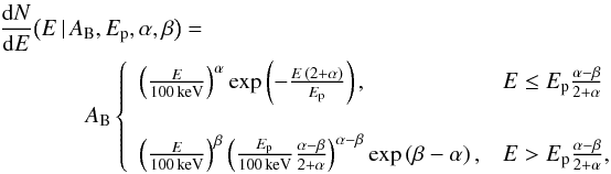$\begin{array}{ccc}& & \frac{\mathrm{d}\mathit{N}}{\mathrm{d}\mathit{E}}(\mathit{E}\hspace{0.17em}\mathrm{|}\hspace{0.17em}{\mathit{A}}_{\mathrm{B}}\mathit{,}{\mathit{E}}_{\mathrm{p}}\mathit{,\alpha ,\beta })\mathrm{=}\\ & & \end{array}$(1)where α and β are the respective photon indices, and E_p is the peak energy of the spectral energy distribution (SED), $\mathit{\nu }{\mathit{F}}_{\mathit{\nu }}\mathrm{=}{\mathit{E}}^{\mathrm{2}}\frac{\mathrm{d}\mathit{N}}{\mathrm{d}\mathit{E}}$.

In the LAT energy range, we adopted either a power law (hereafter PL), a power law with exponential cutoff (CUTPL), or a broken power law with exponential cutoff (CUTBPL). The CUTBPL function has three free parameters (A_C, γ and E_f) and is defined as 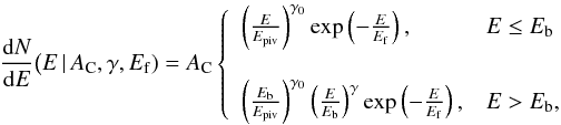$\frac{\mathrm{d}\mathit{N}}{\mathrm{d}\mathit{E}}(\mathit{E}\hspace{0.17em}\mathrm{|}\hspace{0.17em}{\mathit{A}}_{\mathrm{C}}\mathit{,\gamma ,}{\mathit{E}}_{\mathrm{f}}\mathrm{)}\mathrm{=}{\mathit{A}}_{\mathrm{C}}\{\begin{array}{c}\\ {\left(\frac{\mathit{E}}{{\mathit{E}}_{\mathrm{piv}}}\right)}^{{\mathit{\gamma }}_{\mathrm{0}}}\exp \mathrm{(}\mathrm{-}{\frac{\mathit{E}}{{\mathit{E}}_{\mathrm{f}}}}^{\mathrm{)}}\mathit{,}& \mathit{E}\mathrm{\le }{\mathit{E}}_{\mathrm{b}}\\ \\ {\left(\frac{{\mathit{E}}_{\mathrm{b}}}{{\mathit{E}}_{\mathrm{piv}}}\right)}^{{\mathit{\gamma }}_{\mathrm{0}}}{\mathrm{(}{\frac{\mathit{E}}{{\mathit{E}}_{\mathrm{b}}}}^{\mathrm{)}}}^{\mathit{\gamma }}\exp \mathrm{(}\mathrm{-}{\frac{\mathit{E}}{{\mathit{E}}_{\mathrm{f}}}}^{\mathrm{)}}\mathit{,}& \mathit{E}\mathit{>}{\mathit{E}}_{\mathrm{b}}\mathit{,}\end{array}$(2)where γ is the photon index and E_f is the folding energy of the exponential cutoff that characterizes the high-energy spectral break. At low energies, the break at E_b = 200 keV and the photon spectral index γ₀ = + 4 have been fixed to ensure that the flux in the keV−MeV domain is negligible with respect to the flux from the Band spectral component, as expected from an emission spectrum that consists of a synchrotron component in the keV−MeV domain and an inverse Compton component at higher energies (see Sect. 3.2). Specifically, the break energy E_b was fixed to the value that is obtained when this parameter is left free to vary. In order to minimize the correlation between the fitted parameters, the pivot energy E_piv was chosen close to the decorrelation energy. This was fixed to a value between 200 MeV and 500 MeV in the LAT-only spectral analyses and to 10 MeV (time interval c) or 100 MeV (time interval d) in the GBM-LAT joint spectral fits.

The general formulation in Eq. (2) defines the PL and CUTPL functions as subsets of the CUTBPL function. The CUTPL function is obtained in the limit E_b → 0 and the amplitude parameter is redefined as A_C → A′ = A_C(E_b/E_piv)^γ₀. It has three free parameters (A′, γ, and E_f) as follows: 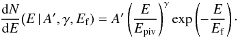$\frac{\mathrm{d}\mathit{N}}{\mathrm{d}\mathit{E}}(\mathit{E}\hspace{0.17em}\mathrm{|}\hspace{0.17em}{\mathit{A}}^{\mathrm{\prime }}\mathit{,\gamma ,}{\mathit{E}}_{\mathrm{f}}\mathrm{)}\mathrm{=}{\mathit{A}}^{\mathrm{\prime }}{\left(\frac{\mathit{E}}{{\mathit{E}}_{\mathrm{piv}}}\right)}^{\mathit{\gamma }}\exp \left(\mathrm{-}\frac{\mathit{E}}{{\mathit{E}}_{\mathrm{f}}}\right)\mathrm{·}$(3)The PL function is obtained by further imposing E_f → + ∞ (1 TeV in practice), leaving two free parameters (A′ and γ) as follows: 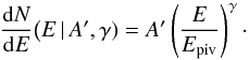$\frac{\mathrm{d}\mathit{N}}{\mathrm{d}\mathit{E}}(\mathit{E}\hspace{0.17em}\mathrm{|}\hspace{0.17em}{\mathit{A}}^{\mathrm{\prime }}\mathit{,\gamma }\mathrm{)}\mathrm{=}{\mathit{A}}^{\mathrm{\prime }}{\left(\frac{\mathit{E}}{{\mathit{E}}_{\mathrm{piv}}}\right)}^{\mathit{\gamma }}\mathrm{·}$(4)In the analyses presented in Sect. 3, we estimated the significance of the high-energy spectral break by fitting models with and without an exponential cutoff at the highest energies. For the LAT-only spectral analysis (Sect. 2.2), we computed the test statistic TS = 2 (lnℒ₁−lnℒ₀), where ℒ₀ and ℒ₁ are the maximum values of the likelihood functions obtained with the PL and CUTPL models, respectively. For the joint GBM-LAT spectral analysis (Sect. 2.3), TS is simply given by the decrease in Castor fit statistic ΔC_stat when an exponential cutoff (i.e., the E_f parameter) is added to the high-energy power-law component of the spectral model. In the large sample limit, TS is equal to the square of the spectral break significance, thus we approximated the latter as ${\mathit{N}}_{\mathit{\sigma }}\mathrm{\simeq }\sqrt{\mathit{TS}}$.

3. Results

This section presents the results of our spectral analyses. More information on the spectral fits are given in Tables A.1−A.6. Firstly, we performed a spectral analysis of GRB 090926A using LAT-only data over the burst duration at high energy and focusing on the time interval c (Sect. 3.1). Then, we performed a time-resolved spectral analysis of GRB 090926A through joint fits to the GBM and LAT data during the time intervals c and d, revealing the time evolution of the high-energy spectral break (Sects. 3.2.1 and 3.2.2). We carefully studied the stability of these results with respect to the systematic uncertainty on the LAT response (Sect. 3.2.3). Finally, we estimated the variability timescales in time intervals c and d and for the GBM and LAT energy ranges (Sect. 3.3), which are needed for the theoretical interpretation presented in the next section.

3.1. LAT-only spectral analysis

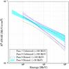Fig. 2 GRB 090926A time-averaged spectral energy distribution as measured by the Fermi/LAT, using Pass 7 data above 100 MeV (dot-dashed butterfly) and Pass 8 data above 30 MeV (filled butterfly) or 100 MeV (dotted and dashed butterflies). Each spectrum is represented by a 68% confidence level contour derived from the errors on the parameters of the fitted power-law function.

We first characterized the time-averaged spectrum of GRB 090926A using LAT Pass 7 and Pass 8 data above 100 MeV during the ${\mathit{T}}_{\mathrm{90}}^{\mathrm{LAT}}$ time interval. We fitted the spectrum with a PL model using the unbinned ML method with Pass 7 data and the unbinned and binned ML methods with Pass 8 data. As shown in Table A.1, all of the three fits gave consistent results in terms of photon index and integrated flux above 100 MeV. Using Pass 8 data yielded spectral parameters that are slightly more constrained. A better accuracy was reached by applying the binned ML analysis to Pass 8 data including events with energies down to 30 MeV (see the last column of Table A.1). The number of events was ~2.3 times higher in this configuration, yielding a photon index γ = −2.20 ± 0.03 and an integrated flux of (48 ± 1.5) × 10^-5cm^-2 s^-1. Figure 2 shows the SED of GRB 090926A for the four analyses described above and their excellent agreement. The narrowest confidence level contour, shown as a filled butterfly in the figure, is obtained for the last fit, which clearly illustrates the improvement of the spectral reconstruction with Pass 8 data above 30 MeV.

Then, we focused our analysis on the time interval c, where the high-energy spectral break of GRB 090926A was initially found (Ackermann et al. 2011). We fitted the spectrum with PL and CUTPL models using the same ML methods and data sets as for the analyses of the ${\mathit{T}}_{\mathrm{90}}^{\mathrm{LAT}}$ time interval described above. As shown in Table A.2, the precision on the fitted photon index is poor owing to the low event statistics above 100 MeV. Moreover, no significant spectral break was found in these analyses. However, the binned ML analysis of Pass 8 data above 30 MeV yields a marginal detection (N_σ = 4.4) with a folding energy ${\mathit{E}}_{\mathrm{f}}\mathrm{=}\mathrm{0.4}{\mathrm{1}}_{-0.14}^{\mathrm{+}\mathrm{0.27}}$ GeV and a photon index γ = −1.68 ± 0.22. These values are affected by large errors and they are fully compatible with the more accurate measurements reported in Ackermann et al. (2011), which were obtained using GBM and LAT data in a joint spectral fit.

3.2. Joint GBM-LAT spectral analysis

3.2.1. Spectrum representation

The results presented in Sect. 3.1 indicate that the high-energy spectral break of GRB 090926A is hard to detect with LAT-only data. Therefore, we considered GBM and LAT data in a joint spectral fit to bring in additional constraints on the photon index of the high-energy component and to increase the sensitivity to any possible spectral break. Starting with a single Band component in the spectral model, we reanalyzed the three time intervals b, c, and d with GBM and LAT Pass 7 or Pass 8 data. Then, we increased the complexity of the model by adding an extra high-energy PL component or a CUTPL component to search for the presence of a spectral break. As was found by Ackermann et al. (2011), the extra PL component was determined to be very significant in the time intervals c and d only. Nevertheless, we searched for a possible spectral break in the time interval b, i.e., we added an exponential attenuation to the high-energy power-law branch of the Band component. We found that a spectral break is not required by the data and that the Band model is enough to reproduce the spectrum of GRB 090926A in this time interval.

In time interval c, the comparison of the Band+PL and Band+CUTPL joint fits confirmed the presence of a high-energy spectral break in the extra PL. Not surprisingly, the evidence for this break was found to be the highest using LAT Pass 8 data above 30 MeV in the spectral fit, i.e., the best LAT data set with the widest spectral coverage. As shown in Table A.3 and Fig. A.1 (top panel), the break significance increased from N_σ = 5.9 with Pass 7 data above 100 MeV to N_σ = 7.7 with Pass 8 data above 30 MeV. Moreover, both the photon index $\mathit{\gamma }\mathrm{=}\mathrm{-}\mathrm{1.6}{\mathrm{8}}_{-0.03}^{\mathrm{+}\mathrm{0.04}}$ and the folding energy ${\mathit{E}}_{\mathrm{f}}\mathrm{=}\mathrm{0.3}{\mathrm{7}}_{-0.05}^{\mathrm{+}\mathrm{0.06}}$ GeV of the CUTPL component were very well constrained in the latter case. These values are compatible with the results reported in Ackermann et al. (2011), $\mathit{\gamma }\mathrm{=}\mathrm{-}\mathrm{1.7}{\mathrm{1}}_{-0.05}^{\mathrm{+}\mathrm{0.02}}$ and ${\mathit{E}}_{\mathrm{f}}\mathrm{=}\mathrm{0.4}{\mathrm{0}}_{-0.06}^{\mathrm{+}\mathrm{0.13}}$ GeV.

In time interval d, a marginal detection of a spectral break (N_σ ~ 4) was reported in Ackermann et al. (2011) with ${\mathit{E}}_{\mathrm{f}}\mathrm{=}\mathrm{2.}{\mathrm{2}}_{-0.7}^{\mathrm{+}\mathrm{0.9}}$ GeV. As shown in Table A.4 and in Fig. A.1 (bottom panel), we found a similar significance of N_σ = 4.3 when using LAT Pass 7 data above 100 MeV in the joint spectral fit. Using instead Pass 8 data above 30 MeV, the significance increased to N_σ = 5.8. This Band+CUTPL fit yielded a photon index, $\mathit{\gamma }\mathrm{=}\mathrm{-}\mathrm{1.7}{\mathrm{5}}_{-0.03}^{\mathrm{+}\mathrm{0.02}}$, which is similar to the photon index found in the time interval c, and a folding energy ${\mathit{E}}_{\mathrm{f}}\mathrm{=}\mathrm{1.6}{\mathrm{1}}_{-0.31}^{\mathrm{+}\mathrm{0.38}}$ GeV, which is significantly higher. These results reveal, for the first time, that the spectral attenuation persists at later times, with an increase of the break characteristic energy up to the GeV domain, and until the end of the keV−MeV prompt emission phase of GRB 090926A, as measured by the GBM.

In Sect. 4, we discuss our results in terms of keV−MeV synchroton radiation of electrons accelerated during the dissipation of the jet energy and inverse Compton emission at higher energies. In this theoretical framework, the inverse Compton component is not expected to contribute significantly to the flux at the lowest energies. The Band+CUTPL representation of GRB 090926A spectra, which we used in the aforementioned analyses, does not meet this requirement, since the extrapolation of the CUTPL component down to ~10 keV yields a flux that is comparable to the flux of the Band component (see Fig. A.1 in this paper and Fig. 5 in Ackermann et al. 2011). Conversely, the CUTBPL component (see Sect. 2.4) is more physically motived. For these reasons, we repeated the joint spectral fits in the time intervals c and d, using LAT Pass 8 data above 30 MeV and adopting the Band+CUTBPL model.

As shown in the last two rows of Table 2, the choice of the Band+CUTBPL model as the best representation of GRB 090926A spectra is justified by its ability to reproduce the data adequately in the time intervals c and d. We investigated different representations of the spectral break, for example, trying to reproduce the more complex shape predicted in Fig. 6 of Hascoët et al. (2012), which consists of a broken power law with an exponential attenuation at higher energies. However, and similar to the analysis reported in Ackermann et al. (2011), the limited photon statistics prevented us from characterizing the shape of this spectral attenuation better than with the Band+CUTBPL model. The Castor fit statistics obtained with the Band+CUTBPL model are only slightly larger that those obtained with the Band+CUTPL model (ΔC_stat = 15.9 and 12.1 for time intervals c and d, respectively). In addition, the spectral parameters remained essentially unchanged, the main difference being observed for the Band photon index α, as expected from the different contributions of the CUTPL and CUTBPL components to the low-energy flux. This parameter decreased from α ~ −0.6 (Band+CUTPL model; see Tables A.3 and A.4) to α ~ −0.9 (Band+CUBTPL model). Both values are higher than the theoretical prediction α = −3/2 for pure fast-cooling synchrotron (Sari et al. 1998), whereas this regime is required to explain the high temporal variability and to reach a high radiative efficiency that is compatible with the huge observed luminosities. The value α ~ −0.6 is difficult to reconcile with synchrotron radiation, except by invoking the marginally fast-cooling regime (Daigne et al. 2011; Beniamini & Piran 2013). The value α ~ −0.9 found in the Band+CUTBPL model is in better agreement, as it is well below the synchrotron death line, α = −2/3, and very close to the limit α ~ −1 that is expected in the fast-cooling regime affected by inverse Compton scatterings in the Klein Nishina regime (Daigne et al. 2011). At high energy, the CUTBPL component is slightly harder than the CUTPL component with a fitted photon index $\mathit{\gamma }\mathrm{=}\mathrm{-}\mathrm{1.4}{\mathrm{8}}_{-0.08}^{\mathrm{+}\mathrm{0.09}}$ (resp. $\mathrm{-}\mathrm{1.7}{\mathrm{1}}_{-0.05}^{\mathrm{+}\mathrm{0.05}}$) in the time interval c (resp. d), whereas the folding energy ${\mathit{E}}_{\mathrm{f}}\mathrm{=}\mathrm{0.3}{\mathrm{4}}_{-0.05}^{\mathrm{+}\mathrm{0.07}}$ GeV (resp. $\mathrm{1.2}{\mathrm{0}}_{-0.18}^{\mathrm{+}\mathrm{0.22}}$ GeV) and its significance N_σ = 7.6 (resp. 6.1) are close to those previously obtained from the Band+CUTPL fit to the data.

3.2.2. Time evolution of the high-energy spectral break

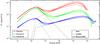Fig. 3 GRB 090926A spectral energy distributions as measured by the Fermi GBM and LAT in time intervals c (red curves), d1 (green curves), and d2 (blue curves) with LAT Pass 8 data above 30 MeV. Each solid curve represents the best-fitted spectral shape (Band+CUTBPL) within a 68% confidence level contour derived from the errors on the fit parameters.

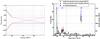Fig. 4 Left: containment interval of the relative systematic uncertainty on the LAT effective area (blue curves) as a function of the photon energy E, and the two ϵ(E) functions used to estimate the corresponding distortion effect on our spectral analysis (red curves). Right: folding energies for the time intervals c, d1, and d2, obtained with or without considering the systematic uncertainties on the LAT effective area. The results were superimposed onto the LAT counts light curve above 30 MeV.

The time evolution of the spectral break characteristic energy in the extra power-law component of GRB 090926A is a novel result that has been made possible thanks to the improved event statistics in the LAT Pass 8 data set. We further investigated this spectral evolution by splitting the time intervals c and d, either by dividing them into two subintervals of equal statistics or by isolating the rising and decaying parts in the corresponding light curves. Then, we performed a Band+CUTBPL fit using the same procedure as in Sect. 3.2.1.

The results of these four fits are reported in Tables A.5 and A.6. No time evolution was found within the interval c, in particular between the two subintervals of equal statistics, in which the high-energy spectral break was detected with high significance (N_σ ≥ 5). Conversely, the high-energy spectral break was found to evolve within the time interval d with a significance between 4.1 and 5.3 depending on the splitting method. In the following, we retained the pair of subintervals with equal statistics, d₁ (from 10.5 s to 12.9 s post-trigger) and d₂ (from 12.9 s to 21.6 s post-trigger). The results of the Band+CUTBPL fits to GBM and LAT data during these time intervals are summarized in Table 2. As for the time intervals c and d, the Band+CUTBPL model was found to reproduce the data adequately. Between d₁ and d₂, the folding energy E_f increased from $\mathrm{0.5}{\mathrm{5}}_{-0.10}^{\mathrm{+}\mathrm{0.13}}$ GeV (with a significance N_σ = 4.3) to $\mathrm{1.4}{\mathrm{3}}_{-0.25}^{\mathrm{+}\mathrm{0.49}}$ GeV (N_σ = 5.1). The final SEDs for the time intervals c, d₁, and d₂, are represented in Fig. 3, where the increase of the high-energy spectral break from 0.34 GeV (interval c) to 1.43 GeV (interval d₂) is clearly visible.

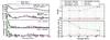Fig. 5 Left: GBM and LAT light curves for GRB 090926A with a 0.02 s time binning. The data from the GBM NaI and BGO detectors were selected from two energy bands, 14.3−260 keV and 260 keV−5 MeV, respectively. The last two panels show the LAT light curves above 30 MeV and 100 MeV, respectively. Right: peak time tpeak and variability timescale tv measured for the time intervals c (red) and d1 (green) in the NaI, BGO, and LAT energy bands.

3.2.3. Systematic effects

The measurements of the high-energy spectral break of GRB 090926A can be affected by systematic uncertainties due to the incomplete knowlege of the LAT instrument response functions (IRFs), namely the LAT effective area, point spread function and energy redistribution function. As explained in the FSSC documentation⁵, the LAT collaboration has estimated the precision of the instrument simulation by performing several consistency checks between IRF predictions and data taken from bright gamma-ray sources (the Vela pulsar, bright active galactic nuclei, and the Earth’s limb). The systematic uncertainty on the effective area is dominant for spectral analyses that account for energy dispersion, especially below 100 MeV. The maximum amplitude of this systematic effect has been parameterized as a function of the photon energy E, as represented by the blue curves in the left panel of Fig. 4. Therefore, we assessed the impact of the systematic effect on the effective area A_eff(E) by replacing it with A_eff(E) [1 + ϵ(E)] in the joint spectral fits, where the chosen uncertainty amplitude ϵ(E) was constrained within this containment interval. The two ϵ(E) functions shown in red in the left panel of Fig. 4 were found to cause the largest spectral distortion. The folding energies E_f for the time intervals c, d₁, and d₂, obtained with or without twisting the effective area, are shown in the right panel of Fig. 4. As can be seen from this figure, the systematic uncertainty on the LAT effective area does not significantly affect the results because the observed changes in E_f are negligible with respect to their statistical errors. In particular, it is worth noting that the confidence intervals on E_f in the different time intervals still exclude each other after modifying the effective area.

3.3. Estimation of the variability timescale

The determination of the bulk Lorentz factor of GRB 090926A is performed in Sect. 4 through the computation of the photon opacity to pair creation, which requires a good estimate of the variability timescale, t_v, in all time intervals. For this purpose, we built the light curves for each time interval and in four energy bands with the summed NaI data (14−260 keV), the BGO data (260 keV−5 MeV), and the LAT data (30 MeV−10 GeV and 100 MeV−10 GeV). The first two energy ranges were chosen as in Ackermann et al. (2011). Following Norris et al. (2005), we then fitted each light curve with a temporal profile that is defined as the product of two exponentials, i.e., 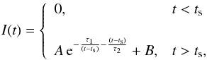$\mathit{I}\mathrm{\left(}\mathit{t}\mathrm{\right)}\mathrm{=}\{\begin{array}{c}\\ \mathrm{0}\mathit{,}& \mathit{t}\mathit{<}{\mathit{t}}_{\mathrm{s}}\\ \\ \mathit{A}\hspace{0.17em}{\mathrm{e}}^{\mathrm{-}\frac{{\mathit{\tau }}_{\mathrm{1}}}{\mathrm{(}\mathit{t}\mathrm{-}{\mathit{t}}_{\mathrm{s}}\mathrm{)}}\mathrm{-}\frac{\mathrm{(}\mathit{t}\mathrm{-}{\mathit{t}}_{\mathrm{s}}\mathrm{)}}{{\mathit{\tau }}_{\mathrm{2}}}}\mathrm{+}\mathit{B,}& \mathit{t}\mathit{>}{\mathit{t}}_{\mathrm{s}}\mathit{,}\end{array}$(5)where A is a normalization factor, t_s is the starting time, τ₁ and τ₂ are related to the peak time ${\mathit{t}}_{\mathrm{peak}}\mathrm{=}\sqrt{{\mathit{\tau }}_{\mathrm{1}}{\mathit{\tau }}_{\mathrm{2}}}$, and the constant parameter B accounts for the background in each detector. We used a simple χ² statistic to check the quality of the fits, and we computed the variability timescale as the half width at half maximum, 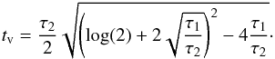$\begin{array}{ccc}{\mathit{t}}_{\mathrm{v}}\mathrm{=}\frac{{\mathit{\tau }}_{\mathrm{2}}}{\mathrm{2}}\sqrt{{\left(\log \mathrm{\left(}\mathrm{2}\mathrm{\right)}\mathrm{+}\mathrm{2}\sqrt{\frac{{\mathit{\tau }}_{\mathrm{1}}}{{\mathit{\tau }}_{\mathrm{2}}}}\right)}^{\mathrm{2}}\mathrm{-}\mathrm{4}\frac{{\mathit{\tau }}_{\mathrm{1}}}{{\mathit{\tau }}_{\mathrm{2}}}}\mathrm{·}& & \end{array}$The left panel of Fig. 5 shows the light curves from the beginning of the time interval c to the end of the time interval d₁, along with their temporal fits. The corresponding values of t_peak and t_v are reported in the right panel of the same figure. In the time interval c, our results confirm the remarkable synchronization of the bright spike across the whole spectrum with t_peak = 9.93 ± 0.01 s in all detectors. The variability timescales for this time interval is t_v = 0.10 ± 0.01 s in the NaI and BGO energy ranges and t_v = 0.06 ± 0.01 s in the two LAT energy ranges. In the time interval d₁, the timescale decreases from 1.13 ± 0.04 s (NaI) to 0.6 ± 0.1 s (BGO) and 0.4 ± 0.2 s (LAT). In both cases, the measured GeV variability timescales thus appear to be similar to those in the MeV energy range. The LAT light curve for the time interval d₂ was not structured enough and was too difficult to fit. Conversely, the NaI light curve consists of two different pulses that we fitted with two temporal profiles. Only the BGO light curve contains a single pulse at t_peak = 13 ± 0.1 s with a variability timescale t_v = 0.5 ± 0.1 s.

4. Interpretation and discussion

4.1. Context

If the high-energy spectral break observed in the time intervals c, d₁, and d₂ is an actual cutoff resulting from pair production γγ → e⁺e⁻, it can be used to estimate the value of the Lorentz factor Γ of the emitting material (Krolik & Pier 1991; Baring & Harding 1997; Lithwick & Sari 2001; Granot et al. 2008; Hascoët et al. 2012). However, the possibility that this spectral break could correspond to a natural curvature in the spectrum of the inverse Compton process in the Klein-Nishina regime (natural break hereafter) cannot be entirely excluded, and only a lower limit on Γ can be obtained in this case. We consider below these two possibilities in two different scenarios: (i) the GRB prompt emission in the GBM range is produced in the optically thin regime above the photosphere or (ii) this prompt emission is produced at the photosphere, as proposed in the dissipative photosphere model (Eichler & Levinson 2000; Rees & Mészáros 2005; Pe’er et al. 2006; Beloborodov 2010, 2013). In case (i), the radius at which the MeV photons are produced is given by 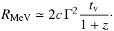${\mathit{R}}_{\mathrm{MeV}}\mathrm{\simeq }\mathrm{2}\mathit{c}\hspace{0.17em}{\mathrm{\Gamma }}^{\mathrm{2}}\frac{{\mathit{t}}_{\mathrm{v}}}{\mathrm{1}\mathrm{+}\mathit{z}}\mathrm{·}$(6)This estimate corresponds to the internal shock scenario (Rees & Mészáros 2005; Kobayashi et al. 1997; Daigne & Mochkovitch 1998) but a comparable radius is expected in some magnetic reconnection models such as ICMART (Zhang & Yan 2011). In both scenarios (i) and (ii) the GeV photons can be emitted from the same location as the MeV photons, R_GeV ≃ R_MeV, which is expected if the variability of the GeV and MeV emissions is comparable (as suggested by our analysis in Sect. 3.3), or from a larger radius R_GeV>R_MeV if they come from the further reprocessing of the MeV photons (Beloborodov et al. 2014) or have an afterglow origin (Ando et al. 2008; Kumar & Barniol Duran 2009, 2010; Ghisellini et al. 2010; Piran & Nakar 2010).

4.2. Case (i): prompt emission produced above the photosphere

4.2.1. Constraints on the Lorentz factor if the high-energy spectral break is due to gamma-ray opacity to pair creation

In this case the radius of the MeV emission is given by Eq. (6) above. If the high-energy spectral break is an actual cutoff resulting from photon opacity to pair creation, the Lorentz factor can be directly estimated from the burst parameters (Eq. (59) in Hascoët et al. 2012) as follows: $\begin{array}{ccc}{\mathrm{\Gamma }}_{\mathit{\gamma \gamma }}& \mathrm{=}& \frac{\mathit{K}\hspace{0.17em}\mathrm{\Phi }\mathrm{\left(}\mathit{s}\mathrm{\right)}}{{\mathrm{[}\frac{\mathrm{1}}{\mathrm{2}}\mathrm{(}\mathrm{1}\mathrm{+}{\frac{{\mathit{R}}_{\mathrm{GeV}}}{{\mathit{R}}_{\mathrm{MeV}}}}^{\mathrm{)}}{\mathrm{(}{\frac{{\mathit{R}}_{\mathrm{GeV}}}{{\mathit{R}}_{\mathrm{MeV}}}}^{\mathrm{)}}}^{\mathrm{]}}}^{\mathrm{1}\mathit{/}\mathrm{2}}}\mathrm{(}\mathrm{1}\mathrm{+}\mathit{z}{\mathrm{)}}^{\mathrm{-}\mathrm{(}\mathrm{1}\mathrm{+}\mathit{s}\mathrm{)}\mathit{/}\mathrm{(}\mathrm{1}\mathrm{-}\mathit{s}\mathrm{)}}\\ & & \mathrm{\times }\mathrm{\left\{}{\mathit{\sigma }}_{\mathrm{T}}{\left[\frac{{\mathit{D}}_{\mathrm{L}}\mathrm{\left(}\mathit{z}\mathrm{\right)}}{\mathit{c}{\mathit{t}}_{\mathrm{v}}}\right]}^{\mathrm{2}}{\mathit{E}}_{\mathrm{\ast }}\mathit{F}\mathrm{\right(}{\mathit{E}}_{\mathrm{\ast }}\mathrm{)}{\mathrm{\}}}^{\mathrm{1}\mathit{/}\mathrm{2}\mathrm{(}\mathrm{1}\mathrm{-}\mathit{s}\mathrm{)}}{\left[\frac{{\mathit{E}}_{\mathrm{\ast }}\hspace{0.17em}{\mathit{E}}_{\mathrm{cut}}}{\mathrm{(}{\mathit{m}}_{\mathit{e}}{\mathit{c}}^{\mathrm{2}}{\mathrm{)}}^{\mathrm{2}}}\right]}^{\mathrm{(}\mathit{s}\mathrm{+}\mathrm{1}\mathrm{)}\mathit{/}\mathrm{2}\mathrm{(}\mathit{s}\mathrm{-}\mathrm{1}\mathrm{)}}\mathrm{·}\\ & & \end{array}$The various observed quantities appearing in Eq. (8) are listed in Table 3 for time intervals c, d₁, and d₂: t_v is the observed variability timescale in the considered time interval, estimated in Sect. 3.3; E_cut is the cutoff energy, which we assume here to be equal to the folding energy E_f that characterizes the spectral break (Sect. 3.2), also listed in Table 3; E_∗ is the typical energy of the seed photons interacting with those at the cutoff energy E_cut, s is the photon index of the seed spectrum close to E_∗, and F(E_∗) is the photon fluence at E_∗ integrated over a duration t_v, so that the seed photon spectrum can be approximated by F(E) = F(E_∗)⁽E/E_∗^)s (cm^-2 MeV^-1). The energy E_∗ is given by 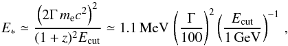${\mathit{E}}_{\mathrm{\ast }}\mathrm{\simeq }\frac{{\mathrm{(}\mathrm{2}\mathrm{\Gamma }\hspace{0.17em}{\mathit{m}}_{\mathrm{e}}{\mathit{c}}^{\mathrm{2}}\mathrm{)}}^{\mathrm{2}}}{\mathrm{(}\mathrm{1}\mathrm{+}\mathit{z}{\mathrm{)}}^{\mathrm{2}}{\mathit{E}}_{\mathrm{cut}}}\mathrm{\simeq }\mathrm{1.1}\hspace{0.17em}\mathrm{MeV}\hspace{0.17em}{\left(\frac{\mathrm{\Gamma }}{\mathrm{100}}\right)}^{\mathrm{2}}{\left(\frac{{\mathit{E}}_{\mathrm{cut}}}{\mathrm{1}\hspace{0.17em}\mathrm{GeV}}\right)}^{-1}\hspace{0.17em}\mathit{,}$(9)where E_∗ and E_cut are the observed values. As the seed photon spectrum is approximated locally by a power law, a precise value of E_∗ is not required, as long as the correct region of the spectrum has been identified. It can be seen that the Lorentz factor Γ_γγ does not depend on a specific choice of E_∗ as long as this energy remains in a region where the spectrum keeps a fixed spectral index s. Indeed E_∗ appears in two factors in Eq. (8) with opposite scaling, ${\left({\mathit{E}}_{\mathrm{\ast }}\mathit{F}\mathrm{\left(}{\mathit{E}}_{\mathrm{\ast }}\mathrm{\right)}\right)}^{\mathrm{1}\mathit{/}\mathrm{2}\mathrm{(}\mathrm{1}\mathrm{-}\mathit{s}\mathrm{)}}\mathrm{\propto }{\mathit{E}}_{\mathrm{\ast }}^{\mathrm{-}\mathrm{(}\mathit{s}\mathrm{+}\mathrm{1}\mathrm{)}\mathit{/}\mathrm{2}\mathrm{(}\mathit{s}\mathrm{-}\mathrm{1}\mathrm{)}}$.For the time interval c, the seed photons belong clearly to the CUTBPL component (see Fig. 3 at ~10 MeV), whereas for the time intervals d₁ and d₂, E_∗ is in the flat transition region of the spectrum where the Band and the CUTBPL components overlap (see Fig. 3). In order to quantify the photon index s, we built its distribution using the results of the spectral fits. Specifically, we assumed that the seven parameters of the Band+CUTBPL spectral model follow a multidimensional Gaussian distribution. Using their covariance matrix provided by the spectral fit, we generated 1000 sets of values for these parameters. For each generated spectrum, we computed numerically the photon index at E_∗. The index s was chosen as the most probable value of the final distribution and its errors were derived from the 68% confidence interval around this value. The corresponding values of F(E_∗) in the table are deduced from the spectral fits presented in Sect. 3.2; the function Φ(s) is defined by $\mathrm{\Phi }\mathrm{\left(}\mathit{s}\mathrm{\right)}\mathrm{=}{\mathrm{\left[}{\mathrm{2}}^{\mathrm{1}\mathrm{+}\mathrm{2}\mathit{s}}\mathrm{ℐ}\mathrm{\right(}\mathit{s}{\mathrm{\left)}}^{\mathrm{\right]}}}^{\frac{\mathrm{1}}{\mathrm{2}\mathrm{(}\mathrm{1}\mathrm{-}\mathit{s}\mathrm{)}}}\hspace{0.17em}\mathit{,}$(10)where ℐ(s) depends on s only and equals (Hascoët et al. 2012) $\mathrm{ℐ}\mathrm{\left(}\mathit{s}\mathrm{\right)}\mathrm{=}{\mathrm{\int }}_{\mathrm{0}}^{\mathrm{1}}\frac{\mathit{y}}{{\left(\mathrm{1}\mathrm{-}{\mathit{y}}^{\mathrm{2}}\right)}^{\mathrm{2}\mathrm{+}\mathit{s}}}\hspace{0.17em}\mathit{g}\mathrm{\left(}\mathit{s}\mathrm{\right)}\hspace{0.17em}\mathrm{d}\mathit{s}\hspace{0.17em}\mathit{,}$(11)with $\mathit{g}\mathrm{\left(}\mathit{y}\mathrm{\right)}\mathrm{=}\frac{\mathrm{3}}{\mathrm{16}}\mathrm{(}\mathrm{1}\mathrm{-}{\mathit{y}}^{\mathrm{2}}\mathrm{)}\left[\mathrm{(}\mathrm{3}\mathrm{-}{\mathit{y}}^{\mathrm{4}}\mathrm{)}\ln \frac{\mathrm{1}\mathrm{+}\mathit{y}}{\mathrm{1}\mathrm{-}\mathit{y}}\mathrm{-}\mathrm{2}\mathit{y}\mathrm{(}\mathrm{2}\mathrm{-}{\mathit{y}}^{\mathrm{2}}\mathrm{)}\right]$ coming directly from the dependence of the γγ cross section on the energy.

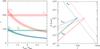Fig. 6 Left: Lorentz factor Γγγ for the time intervals c (red), d1 (blue), and d2 (green) as a function of the ratio of the emission radii of the GeV and MeV photons, assuming that the high-energy spectral break comes from photon opacity to pair creation (Eq. (8)). The dashed lines represent the lower limit of the Lorentz factor for transparency, Γtr (Eq. (13)). The shaded strips indicate the typical uncertainty on these quantities, obtained by propagating the errors on the measured values listed in Table 3. Right: MeV (full lines) and GeV (dashed lines) emission radii as a function of the Lorentz factor. The dotted lines correspond to the photospheric radius Rph in the different time intervals. The deceleration radius is not plotted, but we checked that it is always well above Rph, RMeV, and RGeV for normal densities in the external medium (assuming either a wind or a uniform medium).

Finally, the constant K appearing in front of Eq. (8) has been calibrated by Hascoët et al. (2012) from a detailed time-dependent calculation of the γγ opacity taking into account a realistic geometry for the radiation field, i.e., a time-, space- and direction-dependent photon field in the comoving frame, as expected in an outflow with several emitting zones that are moving relativistically. This calculation, first carried out analytically by Granot et al. (2008) and then extended numerically by Hascoët et al. (2012), is much more realistic than the simple one-zone model that is used, for instance, by Lithwick & Sari (2001). The detailed calculation assumes that the Lorentz factor in the outflow varies between a lowest value Γ_min and a highest value κ Γ_min. If the contrast is on the order of κ ~ 2−5,the calibration factor remains in the interval K ~ 0.4−0.5. In such a variable outflow, the value of Γ_γγ obtained from Eq. (8) corresponds to the lowest Lorentz factor Γ_min in the outflow (Hascoët et al. 2012).

Table 3 provides the resulting Lorentz factor assuming an equal radius for GeV and MeV emissions. If the GeV photons are produced at R_GeV>R_MeV, the Lorentz factor is lower, as can be seen from Eq. (8). The result for each time interval is plotted in Fig. 6 (left panel). For R_GeV = R_MeV (as suggested by the comparable variability timescales in the LAT and the MeV range, see Sect. 3.3), we find Γ_min = Γ_γγ = 233 ± 18, 100 ± 8 and 98 ± 9 for time intervals c, d₁, and d₂, respectively. In the time interval c, our value is very close to the result of Ackermann et al. (2011), Γ ≃ 220, obtained from a similar analysis based on the detailed analytical approach developed in Granot et al. (2008). Table 3 also provides the resulting emission radius R_MeV, which is on the order of 10¹⁴ cm.

These values for the lowest Lorentz factor in the outflow Γ_min have to be compared with the lower limits on the Lorentz factor for transparency to Thomson scattering on primary electrons and pair-produced leptons, which corresponds to the assumed condition that the prompt emission is produced above the photosphere. This condition reads R_MeV ≥ R_ph, with the photospheric radius given by (Beloborodov 2013) ${\mathit{R}}_{\mathrm{ph}}\mathrm{\simeq }\frac{{\mathit{\sigma }}_{\mathrm{T}}\mathrm{(}\mathrm{1}\mathrm{+}\mathit{f}\mathrm{\pm }\mathrm{)}\hspace{0.17em}\mathit{Ė}}{\mathrm{8}\mathit{\pi }{\mathit{c}}^{\mathrm{3}}{\mathit{m}}_{\mathrm{p}}{\mathrm{\Gamma ̅}}^{\mathrm{3}}\mathrm{(}\mathrm{1}\mathrm{+}\mathit{\sigma }\mathrm{)}}\hspace{0.17em}\mathit{,}$(12)where is the average Lorentz factor in the flow, which we approximate by $\mathrm{\Gamma ̅}\mathrm{=}\frac{\mathrm{1}\mathrm{+}\mathit{\kappa }}{\mathrm{2}}{\mathrm{\Gamma }}_{\min }$, where κ is the contrast defined above; σ_T is the Thomson cross section; f ± the ratio of the number of pairs to primary electrons; Ė the total power injected in the flow; and σ its magnetization at large radius, where the prompt emission is produced, so that Ė/ (1 + σ) is the kinetic power. We checked that for the values of the parameters in Table 3 the optical depth for pair creation is less than unity at R_MeV. Therefore we adopt f ± = 0 in Eqs. (12) and (13). We also assume σ ≪ 1, which is expected for internal shocks. In magnetic reconnection models, if σ is large, R_ph is lower and the transparency condition is more easily satisfied. The power Ė is estimated from the gamma-ray luminosity L listed in Table 3 by Ė = L/ϵ_rad assuming a prompt emission efficiency ϵ_rad = 0.1. Table 3 provides the photospheric radius R_ph using the measurement of the Lorentz factor obtained from the γγ constraint. It can be seen that for R_GeV ≃ R_MeV (as suggested by the comparable variability timescales in the LAT and the MeV range, see Sect. 3.3), the transparency condition is satisfied in all time intervals c, d₁, and d₂. We obtain an emission radius ~ 10¹⁴ cm and a photospheric radius of a few 10¹³ cm in all time intervals. For R_MeV given by Eq. (6), the transparency condition R_MeV ≥ R_ph yields $\mathrm{\Gamma ̅}\mathit{>}\mathrm{\Gamma ̅}\mathrm{tr}\mathrm{\simeq }{\left[\frac{{\mathit{\sigma }}_{\mathrm{T}}\mathrm{(}\mathrm{1}\mathrm{+}\mathit{f}\mathrm{\pm }\mathrm{)}\hspace{0.17em}\mathit{Ė}}{\mathrm{8}\mathit{\pi }{\mathit{c}}^{\mathrm{4}}{\mathit{m}}_{\mathit{p}}\hspace{0.17em}\mathrm{(}\mathrm{1}\mathrm{+}\mathit{\sigma }\mathrm{)}\hspace{0.17em}{\mathit{t}}_{\mathrm{v}}}\right]}^{\mathrm{1}\mathit{/}\mathrm{5}}\mathrm{·}$(13)The resulting Γ_tr is plotted in Fig. 6 (left panel, horizontal dashed lines). It appears clearly that the transparency condition can be fulfilled only if R_GeV/R_MeV ≤ 1.2−1.3. As already mentioned, the comparable variability timescales at low and high energy indeed suggest that R_GeV ≃ R_MeV. When comparing R_MeV and R_ph, the emission radius deduced from the variability timescale is the typical radius where the emission starts. However, the emission continues at larger radii as variations on larger timescales are also observed in the light curves. We conclude from this analysis that GRB 090926A seems fully compatible with the most standard model where the prompt emission is produced by shocks (or reconnection) above the photosphere.

The right panel of Fig. 6, which shows the photospheric and emission (MeV/GeV) radii as a function of the Lorentz factor, basically contains the same information, presented in a different way. Again, the figure clearly shows that observations in the three time intervals are compatible with an emission above the photosphere, as long as the emission radii of the MeV and GeV photons are close to each other. This is consistent with an internal origin for the high-energy component during the prompt phase suggested by the observed variability. We stress that this analysis is largely independent of the precise radiative mechanisms. However, as mentioned in Sect. 3.2.1, a natural candidate is fast-cooling synchrotron radiation for the Band component and inverse Compton scatterings for the CUTBPL component. Therefore, we discuss below the possibility that the observed spectral break is due to the natural curvature of the latter component.

4.2.2. Constraints on the Lorentz factor if the high-energy spectral break is a natural break

If the high-energy spectral break reflects the natural curvature of the inverse Compton spectrum – namely it does not correspond to photon opacity to pair creation but simply results from the spectral shape of the radiative process – then only a lower limit on the Lorentz factor can be obtained. It is given, in each time interval, by ${\mathrm{\Gamma }}_{\inf }\mathrm{=}\max \mathrm{\left(}{\mathrm{\Gamma }}_{\mathit{\gamma \gamma }}\mathit{,}{\mathrm{\Gamma }}_{\mathrm{tr}}\mathrm{\right)}\hspace{0.17em}\mathit{,}$(14)where Γ_γγ is computed by the same Eq. (8) as above, using the maximum energy E_max of the observed photons in the time interval (listed in Table 3) in place of the folding energy E_f. The resulting lower limit on the Lorentz factor is plotted in Fig. 7. It shows that, as soon as R_GeV/R_MeV> 1.3 in the time interval c (resp. 1.5 and 1.2 in the intervals d₁ and d₂), the transparency limit (Eq. (13)) becomes more constraining than the limit on the pair-creation opacity. However, it has already been mentioned that the variability analysis presented in Sect. 3.3 rather suggests R_GeV ≃ R_MeV. In this case, we find lower limits for the Lorentz factor equal to 257 ± 17, 129 ± 8, and 110 ± 8 in time intervals c, d₁, and d₂.

4.3. Case (ii): prompt emission produced at the photosphere

In the case where the prompt emission is produced at the photosphere, the radius of the MeV emission is R_MeV = R_ph, given by Eq. (12) above. The constraints derived from the observed spectral break become more difficult to obtain. Indeed, contrary to the previous case, increasing the Lorentz factor drives the emitting surface inward, contributing to increasing the optical depth for the GeV photons. However pair creation is now expected below and at the photosphere with values of several tens for f ± (Beloborodov 2013), which, on the contrary, would contribute to push the photosphere outward. Moreover, since prompt emission at the photosphere corresponds to lower emission radii R_MeV than in the optically thin scenario, most of the GeV photons could be produced above the photosphere (e.g., at a few R_ph) and still show a short variability timescale (t_v value of a few R_ph/ 2cΓ²). In photospheric models, constraining the Lorentz factor from the high-energy spectral break therefore would require a detailed modeling of the radiative transfer from below to above the photosphere, which is beyond the scope of this paper.

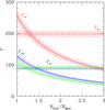Fig. 7 Same as left panel of Fig. 6, but assuming that the observed cutoff is a natural break. The Lorentz factor Γγγ is now a lower limit obtained from the photon of highest energy in each time interval.

4.4. Discussion

It is widely believed that very bright GRBs should have large Lorentz factors. This assumption is based on the pair creation constraint combined with the Fermi/LAT observations of the first bright GRBs (GRBs 080916C, 090510, and 090902B), whose spectrum do not exhibit any attenuation at GeV energies (Abdo et al. 2009b,a; Ackermann et al. 2010). However, later studies (Granot et al. 2008; Hascoët et al. 2012) pointed out that the single-zone model used in these early studies was not accurate enough. Large Lorentz factors are also required in models that assume that the GeV emission is produced at the external shock in order to ensure an early deceleration (Kumar & Barniol Duran 2009; Ghisellini et al. 2010). In the present study of GRB 090926A, we disfavor the external origin scenario because of the observed fast variability of the high-energy emission and find values of the Lorentz factor in the three time intervals reported in Table 3 that are not especially high. From Eq. (8), a lower Lorentz factor and a short variability timescale make the detection of a cutoff due to pair-creation opacity easier since (see, e.g., Dermer et al. 1999) ${\mathit{E}}_{\mathrm{cut}}\mathrm{\propto }{\mathrm{\Gamma }}^{\mathrm{2}\mathrm{(}\mathit{s}\mathrm{-}\mathrm{1}\mathrm{)}\mathit{/}\mathrm{(}\mathit{s}\mathrm{+}\mathrm{1}\mathrm{)}}\hspace{0.17em}{\mathit{t}}_{\mathrm{v}}^{\mathrm{-}\mathrm{2}\mathit{/}\mathrm{(}\mathit{s}\mathrm{+}\mathrm{1}\mathrm{)}}\mathit{,}$(15)giving ${\mathit{E}}_{\mathrm{cut}}\mathrm{\propto }{\mathrm{\Gamma }}^{\mathrm{10}}\hspace{0.17em}{\mathit{t}}_{\mathrm{v}}^{\mathrm{4}}$ and ${\mathit{E}}_{\mathrm{cut}}\mathrm{\propto }{\mathrm{\Gamma }}^{\mathrm{5.3}}\hspace{0.17em}{\mathit{t}}_{\mathrm{v}}^{\mathrm{1.7}}$ for s = −1.5 and −2.2, respectively. This could explain why the cutoff in the time interval c with t_v = 0.1 s, Γ ~ 230 and a very large luminosity was the most easily accessible. With a larger Lorentz factor the cutoff would have been shifted to a much higher energy and would have been difficult to characterize. More generally, the very steep dependence of E_cut with the Lorentz factor means that, for a given burst, a cutoff can be observed in the LAT range for a very small interval in Γ only. This may explain why bursts like GRB 090926A are not common in the LAT catalog.

As mentioned in Sect. 4.2.1, the Lorentz factor that we find in the time interval c is very close to the value obtained by Ackermann et al. (2011) with the time dependent model of Granot et al. (2008). Another way to estimate the Lorentz factor consists in assuming that the peak flux time in the LAT or visible range is a good proxy for the deceleration time of the relativistic ejecta (see, however, Hascoët et al. 2014). With this method Ackermann et al. (2013a) found Γ ≃ 600 (resp. 400) for a uniform external medium of density n = 1 cm^-3 (resp. a stellar wind with a parameter A_∗ = 0.1), assuming a deceleration time t_dec ≃ 10 s and a gamma-ray efficiency f_γ = 0.25. The obtained result depends on these parameters as $\mathrm{\Gamma }\mathrm{\propto }\{\begin{array}{c}\\ & \mathrm{(}{\mathit{f}}_{\mathit{\gamma }}\mathit{n}{\mathrm{)}}^{\mathrm{-}\mathrm{1}\mathit{/}\mathrm{8}}\hspace{0.17em}{\mathit{t}}_{\mathrm{dec}}^{\mathrm{-}\mathrm{3}\mathit{/}\mathrm{8}}\mathrm{uniform}\mathrm{external}\mathrm{medium}\\ & \mathrm{(}{\mathit{f}}_{\mathit{\gamma }}{\mathit{A}}_{\mathrm{\ast }}{\mathrm{)}}^{\mathrm{-}\mathrm{1}\mathit{/}\mathrm{4}}\hspace{0.17em}{\mathit{t}}_{\mathrm{dec}}^{\mathrm{-}\mathrm{1}\mathit{/}\mathrm{4}}\mathrm{stellar}\mathrm{wind}\mathit{,}\end{array}$(16)which shows that an external medium denser than what was assumed by Ackermann et al. (2013a) (e.g., with n = 1000 cm^-3 or A_∗ = 1) or a deceleration time larger than 10 s could reconcile the two approaches. A value of t_dec larger than 10 s is actually very likely, since the peak flux time in the LAT light curve coincides with the spike in time interval c, which probably results from internal dissipation as indicated by its extreme variability.

The evolution of the Lorentz factor from the time interval c to intervals d₁ and d₂ is moderate, showing a decrease by a factor of 2, while the luminosity in the time interval c is 8 times larger and the variability timescale is 5−6 times smaller. The Lorentz factor follows approximately a trend Γ ∝ L^0.3 but clearly, with only three time intervals (and two with very similar temporal and spectral parameters) more data will be needed to check whether this expected behavior (see, e.g., Baring 2006) is also found in other bursts and over large parts of their temporal evolution.

5. Conclusions

We presented a new time-resolved analysis of GRB 090926A broadband spectrum during its prompt phase. We combined the Fermi/GBM and LAT data in joint spectral fits to characterize the time evolution of its spectrum from keV to GeV energies, using a Band+CUTBPL spectral model in view of discussing our results in terms of keV−MeV synchroton radiation of accelerated electrons and inverse Compton emission at higher energies. In this analysis, we made use of the LAT Pass 8 data publicly released in June 2015, which offer a greater sensitivity than any LAT data selection used in previous studies of this burst. Using a Band+CUTBPL model to account for the broadband spectral energy distribution of GRB 090926A, we confirmed and better constrained the spectral break at the time of the bright spike, which is observed at ~10 s post-trigger across the whole spectrum. Our analysis revealed that the spectral attenuation persists at later times, with an increase of the break characteristic energy until the end of the prompt phase, from 0.34 GeV (interval c) to 1.43 GeV (interval d₂). We paid careful attention to the systematic effects arising from the uncertainties on the LAT response, and we showed that this time evolution of the spectral break in the high-energy power-law component of GRB 090926A spectrum is solid and well established.

After computing the variability timescales from keV to GeV energies during and after the bright spike, we discussed our results in the framework of prompt emission models. We interpret the high-energy spectral break as caused by photon opacity to pair creation. Requiring that all emissions are produced above the photosphere of GRB 090926A, we computed the bulk Lorentz factor of the outflow, Γ. The latter decreases from 230 during the spike to 100 at the end of the prompt emission, a novel result that improves upon early publications on this burst (Ackermann et al. 2011). Assuming, instead, that the spectral break reflects the natural curvature of the inverse Compton spectrum, lower limits corresponding to larger values for Γ were also derived. Despite the increased photon statistics provided in LAT Pass 8 data, we could not favor any of these possible scenarios. In both scenarios, the extreme temporal variability of GRB 090926A and the Lorentz factors lead to emission radii R ~ 10¹⁴ cm and to a photospheric radius of a few 10¹³ cm in all time intervals. This strongly suggests an internal origin of both the keV−MeV and GeV prompt emissions associated with internal jet dissipation above the photosphere. This interpretation is reinforced by the flattening of the gamma-ray light curve decay, which occurs well after the end of the keV−MeV prompt emission (Ackermann et al. 2013a), as mentioned in Sect. 1.

In the future, further progress toward the understanding of the GRB GeV emission that coincides with the emergence of an additional power-law component will be possible by using LAT Pass 8 data in broadband analyses of other LAT bright bursts with similar temporal and spectral properties to GRB 090926A, such as the short GRB 090510 (Ackermann et al. 2013a). On the theoretical side, the results obtained in our study and, in general, the complex time evolution of GRB emission spectrum during their prompt phase, also call for the development of detailed broadband physical models to pinpoint which processes dominate during the first instants of the GRB emission and to assess the contribution of internal emission to the GeV spectrum. For instance, our results regarding the photon spectral indices at low energies (α ~ −0.9) and at high energies (γ ~ −1.6) are promising, since they show good agreement with prompt emission models based on fast-cooling electron synchrotron emission with inverse Compton scatterings in the Klein Nishina regime (Bošnjak & Daigne 2014). Dedicated simulations aimed at reproducing GRB 090926A spectral evolution in detail constitute the next step in this direction.

Acknowledgments

The Fermi LAT Collaboration acknowledges generous ongoing support from a number of agencies and institutes that have supported both the development and operation of the LAT as well as scientific data analysis. These include the National Aeronautics and Space Administration and the Department of Energy in the United States, the Commissariat à l’Énergie Atomique and the Centre National de la Recherche Scientifique/Institut National de Physique Nucléaire et de Physique des Particules in France, the Agenzia Spaziale Italiana and the Istituto Nazionale di Fisica Nucleare in Italy, the Ministry of Education, Culture, Sports, Science and Technology (MEXT), High Energy Accelerator Research Organization (KEK) and Japan Aerospace Exploration Agency (JAXA) in Japan, and the K. A. Wallenberg Foundation, the Swedish Research Council and the Swedish National Space Board in Sweden.

Additional support for science analysis during the operations phase is gratefully acknowledged from the Istituto Nazionale di Astrofisica in Italy and the Centre National d’Études Spatiales in France.

The authors would like to thank the Programme National Hautes Énergies for their financial support (PNHE, funded by CNRS/INSU-IN2P3, CEA and CNES, France). They also thank J. Palmerio for his careful reading of the manuscript.

References

Appendix A: Spectral analysis results

In this section we give more information on the spectral analyses reported in Sect. 3.

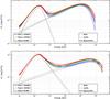Fig. A.1 GRB 090926A spectral energy distributions as measured by the Fermi GBM and LAT in time intervals c(top panel) and d(bottom panel), using LAT Pass7 above 100 MeV, and Pass 8 data above 30 MeV and 100 MeV (see Tables A.3 and A.4 for more details). Each solid curve represents the best-fitted spectral shape (Band+CUTBPL), within a 68% confidence level contour derived from the errors on the fit parameters.

All Tables

All Figures

Fig. 1 GRB 090926A counts light curves as measured by the GBM and LAT, from lowest to highest energies. The sum of the counts in the GBM NaI detectors (first panel), in the GBM BGO detector facing the burst (second panel), and using the LAT Pass 8 transient-class events above 30 MeV within a 12° region of interest (third panel). The last panel shows the energies of the events from this sample, which have been detected above 300 MeV. The dashed blue vertical lines indicate the time intervals that are used for the joint GBM and LAT spectral analyses.

In the text

	Fig. 2 GRB 090926A time-averaged spectral energy distribution as measured by the Fermi/LAT, using Pass 7 data above 100 MeV (dot-dashed butterfly) and Pass 8 data above 30 MeV (filled butterfly) or 100 MeV (dotted and dashed butterflies). Each spectrum is represented by a 68% confidence level contour derived from the errors on the parameters of the fitted power-law function.
In the text

	Fig. 3 GRB 090926A spectral energy distributions as measured by the Fermi GBM and LAT in time intervals c (red curves), d1 (green curves), and d2 (blue curves) with LAT Pass 8 data above 30 MeV. Each solid curve represents the best-fitted spectral shape (Band+CUTBPL) within a 68% confidence level contour derived from the errors on the fit parameters.
In the text

Fig. 4 Left: containment interval of the relative systematic uncertainty on the LAT effective area (blue curves) as a function of the photon energy E, and the two ϵ(E) functions used to estimate the corresponding distortion effect on our spectral analysis (red curves). Right: folding energies for the time intervals c, d1, and d2, obtained with or without considering the systematic uncertainties on the LAT effective area. The results were superimposed onto the LAT counts light curve above 30 MeV.

In the text

Fig. 5 Left: GBM and LAT light curves for GRB 090926A with a 0.02 s time binning. The data from the GBM NaI and BGO detectors were selected from two energy bands, 14.3−260 keV and 260 keV−5 MeV, respectively. The last two panels show the LAT light curves above 30 MeV and 100 MeV, respectively. Right: peak time tpeak and variability timescale tv measured for the time intervals c (red) and d1 (green) in the NaI, BGO, and LAT energy bands.

In the text

Fig. 6 Left: Lorentz factor Γγγ for the time intervals c (red), d1 (blue), and d2 (green) as a function of the ratio of the emission radii of the GeV and MeV photons, assuming that the high-energy spectral break comes from photon opacity to pair creation (Eq. (8)). The dashed lines represent the lower limit of the Lorentz factor for transparency, Γtr (Eq. (13)). The shaded strips indicate the typical uncertainty on these quantities, obtained by propagating the errors on the measured values listed in Table 3. Right: MeV (full lines) and GeV (dashed lines) emission radii as a function of the Lorentz factor. The dotted lines correspond to the photospheric radius Rph in the different time intervals. The deceleration radius is not plotted, but we checked that it is always well above Rph, RMeV, and RGeV for normal densities in the external medium (assuming either a wind or a uniform medium).

In the text

	Fig. 7 Same as left panel of Fig. 6, but assuming that the observed cutoff is a natural break. The Lorentz factor Γγγ is now a lower limit obtained from the photon of highest energy in each time interval.
In the text

Fig. A.1 GRB 090926A spectral energy distributions as measured by the Fermi GBM and LAT in time intervals c(top panel) and d(bottom panel), using LAT Pass7 above 100 MeV, and Pass 8 data above 30 MeV and 100 MeV (see Tables A.3 and A.4 for more details). Each solid curve represents the best-fitted spectral shape (Band+CUTBPL), within a 68% confidence level contour derived from the errors on the fit parameters.

In the text

References

- Abdo, A. A., Ackermann, M., Ajello, M., et al. 2009a, ApJ, 706, L138 [NASA ADS] [CrossRef] [Google Scholar]
- Abdo, A. A., Ackermann, M., Arimoto, M., et al. 2009b, Science, 323, 1688 [Google Scholar]
- Ackermann, M., Asano, K., Atwood, W. B., et al. 2010, ApJ, 716, 1178 [NASA ADS] [CrossRef] [Google Scholar]
- Ackermann, M., Ajello, M., Asano, K., et al. 2011, ApJ, 729, 114 [CrossRef] [Google Scholar]
- Ackermann, M., Ajello, M., Asano, K., et al. 2013a, ApJS, 209, 11 [NASA ADS] [CrossRef] [Google Scholar]
- Ackermann, M., Ajello, M., Asano, K., et al. 2013b, ApJ, 763, 71 [CrossRef] [Google Scholar]
- Ackermann, M., Ajello, M., Asano, K., et al. 2014, Science, 343, 42 [NASA ADS] [CrossRef] [PubMed] [Google Scholar]
- Ando, S., Nakar, E., & Sari, R. 2008, ApJ, 689, 1150 [NASA ADS] [CrossRef] [Google Scholar]
- Atwood, W. B., Abdo, A. A., Ackermann, M., et al. 2009, ApJ, 697, 1071 [NASA ADS] [CrossRef] [Google Scholar]
- Band, D., Matteson, J., Ford, L., et al. 1993, ApJ, 413, 281 [NASA ADS] [CrossRef] [Google Scholar]
- Baring, M. G. 2006, ApJ, 650, 1004 [NASA ADS] [CrossRef] [Google Scholar]
- Baring, M. G., & Harding, A. K. 1997, ApJ, 491, 663 [CrossRef] [Google Scholar]
- Beloborodov, A. M. 2010, MNRAS, 407, 1033 [NASA ADS] [CrossRef] [Google Scholar]
- Beloborodov, A. M. 2013, ApJ, 764, 157 [NASA ADS] [CrossRef] [Google Scholar]
- Beloborodov, A. M., Hascoët, R., & Vurm, I. 2014, ApJ, 788, 36 [NASA ADS] [CrossRef] [Google Scholar]
- Beniamini, P., & Granot, J. 2016, MNRAS, 459, 3635 [NASA ADS] [CrossRef] [Google Scholar]
- Beniamini, P., & Piran, T. 2013, ApJ, 769, 69 [NASA ADS] [CrossRef] [Google Scholar]
- Bošnjak, Ž., & Daigne, F. 2014, A&A, 568, A45 [NASA ADS] [CrossRef] [EDP Sciences] [Google Scholar]
- Daigne, F., & Mochkovitch, R. 1998, MNRAS, 296, 275 [NASA ADS] [CrossRef] [Google Scholar]
- Daigne, F., Bošnjak, Ž., & Dubus, G. 2011, A&A, 526, A110 [NASA ADS] [CrossRef] [EDP Sciences] [Google Scholar]
- De Pasquale, M., Schady, P., Kuin, N. P. M., et al. 2010, ApJ, 709, L146 [NASA ADS] [CrossRef] [Google Scholar]
- Dermer, C. D., Chiang, J., & Böttcher, M. 1999, ApJ, 513, 656 [NASA ADS] [CrossRef] [Google Scholar]
- Eichler, D., & Levinson, A. 2000, ApJ, 529, 146 [NASA ADS] [CrossRef] [Google Scholar]
- Ghisellini, G., Ghirlanda, G., Nava, L., & Celotti, A. 2010, MNRAS, 403, 926 [NASA ADS] [CrossRef] [Google Scholar]
- Giannios, D. 2012, MNRAS, 422, 3092 [NASA ADS] [CrossRef] [Google Scholar]
- Granot, J., Cohen-Tanugi, J., & Silva, E. d. C. e. 2008, ApJ, 677, 92 [NASA ADS] [CrossRef] [Google Scholar]
- Hascoët, R., Daigne, F., Mochkovitch, R., & Vennin, V. 2012, MNRAS, 421, 525 [NASA ADS] [Google Scholar]
- Hascoët, R., Beloborodov, A. M., Daigne, F., & Mochkovitch, R. 2014, ApJ, 782, 5 [NASA ADS] [CrossRef] [Google Scholar]
- Kobayashi, S., Piran, T., & Sari, R. 1997, ApJ, 490, 92 [NASA ADS] [CrossRef] [Google Scholar]
- Krolik, J. H., & Pier, E. A. 1991, ApJ, 373, 277 [NASA ADS] [CrossRef] [Google Scholar]
- Kumar, P., & Barniol Duran, R. 2009, MNRAS, 400, L75 [NASA ADS] [CrossRef] [Google Scholar]
- Kumar, P., & Barniol Duran, R. 2010, MNRAS, 409, 226 [NASA ADS] [CrossRef] [Google Scholar]
- Lemoine, M., Li, Z., & Wang, X.-Y. 2013, MNRAS, 435, 3009 [NASA ADS] [CrossRef] [Google Scholar]
- Lithwick, Y., & Sari, R. 2001, ApJ, 555, 540 [NASA ADS] [CrossRef] [Google Scholar]
- McKinney, J. C., & Uzdensky, D. A. 2012, MNRAS, 419, 573 [Google Scholar]
- Meegan, C., Lichti, G., Bhat, P. N., et al. 2009, ApJ, 702, 791 [NASA ADS] [CrossRef] [Google Scholar]
- Narayana Bhat, P., Meegan, C. A., von Kienlin, A., et al. 2016, ApJS, 223, 28 [Google Scholar]
- Norris, J. P., Bonnell, J. T., Kazanas, D., et al. 2005, ApJ, 627, 324 [NASA ADS] [CrossRef] [Google Scholar]
- Pe’er, A., Mészáros, P., & Rees, M. J. 2005, ApJ, 635, 476 [NASA ADS] [CrossRef] [Google Scholar]
- Pe’er, A., Mészáros, P., & Rees, M. J. 2006, ApJ, 642, 995 [NASA ADS] [CrossRef] [Google Scholar]
- Piran, T. 2004, Rev. Mod. Phys., 76, 1143 [NASA ADS] [CrossRef] [Google Scholar]
- Piran, T., & Nakar, E. 2010, ApJ, 718, L63 [NASA ADS] [CrossRef] [Google Scholar]
- Razzaque, S. 2010, ApJ, 724, L109 [NASA ADS] [CrossRef] [Google Scholar]
- Rees, M. J., & Meszaros, P. 1994, ApJ, 430, L93 [NASA ADS] [CrossRef] [Google Scholar]
- Rees, M. J., & Mészáros, P. 2005, ApJ, 628, 847 [NASA ADS] [CrossRef] [Google Scholar]
- Ryde, F., Pe’er, A., Nymark, T., et al. 2011, MNRAS, 415, 3693 [NASA ADS] [CrossRef] [Google Scholar]
- Sari, R., Piran, T., & Narayan, R. 1998, ApJ, 497, L17 [NASA ADS] [CrossRef] [Google Scholar]
- Vianello, G., Omodei, N., & Fermi/LAT Collaboration. 2015, ArXiv e-prints [arXiv:1502.03122] [Google Scholar]
- Wang, X.-Y., Liu, R.-Y., & Lemoine, M. 2013, ApJ, 771, L33 [NASA ADS] [CrossRef] [Google Scholar]
- Zhang, B., & Yan, H. 2011, ApJ, 726, 90 [NASA ADS] [CrossRef] [Google Scholar]
- Zhang, B., & Zhang, B. 2014, ApJ, 782, 92 [CrossRef] [Google Scholar]