| Issue |
A&A
Volume 604, August 2017
|
|
|---|---|---|
| Article Number | A124 | |
| Number of page(s) | 16 | |
| Section | Galactic structure, stellar clusters and populations | |
| DOI | https://doi.org/10.1051/0004-6361/201730488 | |
| Published online | 25 August 2017 | |
Understanding EROS2 observations toward the spiral arms within a classical Galactic model framework⋆
1 Laboratoire de l’Accélérateur Linéaire, IN2P3-CNRS, Université de Paris-Sud, BP 34, 91898 Orsay Cedex, France
e-mail: moniez@lal.in2p3.fr
2 Department of Physics, Isfahan University of Technology, 84156-83111 Isfahan, Iran
3 Perimeter Institute for Theoretical Physics, 31 Caroline Street North, Waterloo, N2L 2Y5 Ontario, Canada
4 Department of Physics and Astronomy, University of Waterloo, 200 University Avenue West, Waterloo, ON N2L 3G1, Canada
5 Department of Physics, Sharif University of Technology, PO Box 11155-9161, Tehran, Iran
Received: 23 January 2017
Accepted: 10 April 2017
Aims. EROS (Expérience de Recherche d’Objets Sombres) has searched for microlensing toward four directions in the Galactic plane away from the Galactic center. The interpretation of the catalog optical depth is complicated by the spread of the source distance distribution. We compare the EROS microlensing observations with Galactic models (including the Besançon model), tuned to fit the EROS source catalogs, and take into account all observational data such as the microlensing optical depth, the Einstein crossing durations, and the color and magnitude distributions of the catalogued stars.
Methods. We simulated EROS-like source catalogs using the HIgh-Precision PARallax COllecting Satellite (Hipparcos) database, the Galactic mass distribution, and an interstellar extinction table. Taking into account the EROS star detection efficiency, we were able to produce simulated color–magnitude diagrams that fit the observed diagrams. This allows us to estimate average microlensing optical depths and event durations that are directly comparable with the measured values.
Results. Both the Besançon model and our Galactic model allow us to fully understand the EROS color–magnitude data. The average optical depths and mean event durations calculated from these models are in reasonable agreement with the observations. Varying the Galactic structure parameters through simulation, we were also able to deduce contraints on the kinematics of the disk, the disk stellar mass function (at a few kpc distance from the Sun), and the maximum contribution of a thick disk of compact objects in the Galactic plane (Mthick< 5 − 7 × 10¹⁰M⊙ at 95%, depending on the model). We also show that the microlensing data toward one of our monitored directions are significantly sensitive to the Galactic bar parameters, although much larger statistics are needed to provide competitive constraints.
Conclusions. Our simulation gives a better understanding of the lens and source spatial distributions in the microlensing events. The goodness of a global fit taking into account all the observables (from the color-magnitude diagrams and microlensing observations) shows the validity of the Galactic models. Our tests with the parameters excursions show the unique sensitivity of the microlensing data to the kinematical parameters and stellar initial mass function.
Key words: gravitational lensing: micro / Galaxy: structure / Galaxy: kinematics and dynamics / Galaxy: disk / dark matter / stars: luminosity function, mass function
© ESO, 2017
1. Introduction
Following Paczyńskis’ seminal publication (Paczyński 1986), several groups initiated survey programs beginning in 1989 to search for compact halo objects within the Galactic halo. The challenge for the Expérience de Recherche d’Objets Sombres (EROS) and MAssive Compact Halo Objects (MACHO) teams was to clarify the status of the missing hadrons in our own Galaxy. In September 1993, the three teams, EROS (Aubourg et al. 1993), MACHO (Alcock et al. 1993), and Optical Gravitational Lensing Experiment (OGLE; Udalski et al. 1993), discovered the first microlensing events in the directions of the Large Magellanic Cloud and the Galactic center (GC). Since these first discoveries, thousands of microlensing effects have been detected in the direction of the GC together with a handful of events toward the Galactic spiral arms (GSA) and the Magellanic Clouds.
Microlensing has proven to be a powerful probe of the Milky Way structure. Searches for microlensing toward the Magellanic Clouds (LMC, SMC) and M31 (survey MEGA; Crotts & Tomaney 1996 and survey AGAPE; Calchi Novati et al. 2014) provide optical depths through the Galactic halo, allowing one to study dark matter in the form of massive compact objects. Searches toward the Galactic plane (GC and Galactic spiral arms) allow one to measure the microlensing optical depth of ordinary stars in the Galactic disk and bar. Kinematical models and mass functions can also be constrained through the event duration distributions.
Several teams have published results about the Galactic structure, through microlensing searches in the Galactic plane, such as MACHO (Popowski et al. 2005), EROS (Hamadache et al. 2006), OGLE (Sumi et al. 2006), and Microlensing Observations in Astrophysics (MOA; Awiphan et al. 2016). The EROS team is the only group that have searched for microlensing toward the Galactic spiral arms, away from the Galactic center. As a matter of fact, the EROS team have measured the microlensing optical depth toward four directions of the Galactic plane (Fig. 1), i.e.,
-
 ;
; -
γ Nor ( − 2.4°,331.1°);
-
β Sct ( − 2.2°,26.6°);
-
θ Mus ( − 1.5°,306.6°).
as far as 55 degrees in longitude away from the Galactic center (Rahal et al. 2009b).
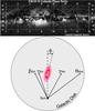 |
Fig. 1 Four directions toward the Galactic spiral arms monitored by EROS. |
The specificity of these measurements with respect to other targets like SMC or LMC is the widespread distribution of the distances of the monitored sources. The distances to the sources could not be individually measured and both their average and dispersion are poorly estimated. The concept of “catalog optical depth” was introduced in Rahal et al. (2009b), and in this paper we describe a complete procedure to compare measured optical depth with model predictions. After the introduction of the microlensing concepts (Sect. 2) and the presentation of the EROS data (Sect. 3), in Sect. 4 we describe the technique to produce synthetic color–magnitude diagrams (CMDs), via the Hipparcos catalog (HIgh-Precision PARallax COllecting Satellite ESA 1997; Turon et al. 1995), the spatial distribution of mass from Galactic models, and the absorptions tabulated in a 3D map obtained with infrared observations (Marshall et al. 2006). We cross-checked the obtained local stellar number densities with the expectations from the stellar initial mass function (IMF). In Sect. 5, we describe the full simulation of the EROS program, in terms of CMDs taking into account the stellar detection efficiency of EROS, and in terms of the microlensing events. Our fitting procedure is described in Sect. 6, where we derive constraints on our simple Galactic model and test the Besançon model (Robin et al. 2003); the fit takes into account the observed CMDs as well as the data from the microlensing (optical depths and mean event durations) toward the four observed lines of sight; we use the fit to estimate the allowed range of our simple Galactic model parameters. In the final discussion (Sect. 7), we extract from the best fit the distance distributions of the sources and lenses. Finally, we discuss the sensitivity of microlensing observations toward the Galactic arms to the dark thick disk, central bar inclination, stellar mass function and disk kinematics.
2. Microlensing effect
The gravitational microlensing effect occurs when a massive compact object passes close enough to the line of sight of a star to produce a temporary magnification of the source. A general overview of the microlensing formalism can be found in Schneider et al. (2006) and Rahvar (2015). In the approximation of a single point-like lens deflecting the light from a single point-like source, the total magnification of the source luminosity at time t is given by (Paczyński 1986)  (1)where u(t) is the distance of the deflecting object to the undeflected line of sight, expressed in units of the Einstein radius RE given by:
 ![\begin{eqnarray} R_{\mathrm{E}} &=& \sqrt{\frac{4GM}{c^2}D_{\rm S} x(1-x)} \\ &\simeq &4.54\ \mathrm{AU} \times\left[\frac{M}{\Msol}\right]^{\frac{1}{2}} \left[\frac{D_{\rm S}}{10~{\rm kpc}}\right]^{\frac{1}{2}} \frac{\left[x(1-x)\right]^{\frac{1}{2}}}{0.5}\cdot \nonumber \end{eqnarray}](/articles/aa/full_html/2017/08/aa30488-17/aa30488-17-eq11.png) (2)Here G is the Newtonian gravitational constant, DS is the distance of the observer to the source, and xDS = DL is its distance to the deflector of mass M. Assuming a deflector moving at a constant relative transverse speed vT, reaching its minimum distance u0 (impact parameter) to the undeflected line of sight at time t0, u(t) is given by
(2)Here G is the Newtonian gravitational constant, DS is the distance of the observer to the source, and xDS = DL is its distance to the deflector of mass M. Assuming a deflector moving at a constant relative transverse speed vT, reaching its minimum distance u0 (impact parameter) to the undeflected line of sight at time t0, u(t) is given by  (3)where tE = RE/vT, the lensing timescale, is the only measurable parameter bringing useful information regarding the lens parameters in the approximation of simple microlensing,
 ![\begin{eqnarray} t_{\mathrm{E}} \sim 79\ \mathrm{days} \times \left[\frac{v_{\rm T}}{100~{\rm km\,s^{-1}}}\right]^{-1} \left[\frac{M}{\Msol}\right]^{\frac{1}{2}} \left[\frac{D_{\rm S}}{10\, {\rm kpc}}\right]^{\frac{1}{2}} \frac{[x(1-x)]^{\frac{1}{2}}}{0.5} \cdot \end{eqnarray}](/articles/aa/full_html/2017/08/aa30488-17/aa30488-17-eq21.png) (4)
(4)
2.1. Microlensing event characteristics
The so-called simple microlensing effect (point-like source and point-like lens with uniform relative motion with respect to the line of sight) has some characteristic features that allow one to discriminate it from any known intrinsic stellar variability. These features are as follows: given the low probability for source detector alignment within RE, the event should be singular in the history of the source (as well as of the deflector); the magnification is independent of the color; the magnification is a simple function of time, depending on (u0,t0,tE), with a symmetrical shape; as the geometric configuration of the source-deflector system is random, the impact parameters of the events must be uniformly distributed; the passive role of the lensed stars implies that their population should be representative of the monitored sample at any given source distance, particularly with respect to the observed color and magnitude distributions.
This simple microlensing description can be complicated in many different ways: for example, multiple lens and source systems (Mao & Stefano 1995), extended sources (Yoo et al. 2004), and parallax effects (Gould 1992); these complications will not be discussed here.
2.2. Observables: optical depth, event rate, and tE distribution
The optical depth up to a given source distance, DS, is defined as the instantaneous probability for the line of sight of a target source to intercept a deflector’s Einstein disk, which corresponds to a magnification A> 1.34. Assuming that the distribution of the deflector masses is described by a density function ρ(DL) and a normalized mass function dnL(DL,M) / dM, this probability is 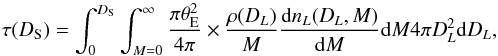 (5)where θE = RE/DL is the angular Einstein radius of a lens of mass M located at DL. The second term of the integral is the differential number of these lenses per mass unit. As the solid angle of the Einstein disk is proportional to the deflectors’ mass M, this probability is found to be independent of the deflectors’ mass function
 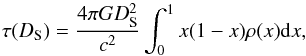 (6)where ρ(x) is the mass density of deflectors located at a distance xDS. This expression is used when the distance to the monitored source population is known (for example, toward the LMC and SMC).
When the monitored population is spread over a wide distance distribution, as is the case toward the Galactic plane, we have to consider the concept of “catalog optical depth” as introduced in Rahal et al. (2009b); the mean optical depth toward a given population defined by a distance distribution dnS(DS) / dDS of target stars is defined as (Moniez 2010) 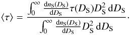 (7)Again, this optical depth does not depend on the deflectors’ mass function. On the other hand, for a given optical depth, the microlensing event rate depends on the deflectors’ mass distribution as well as on the velocity and spatial distributions.
Contrary to the optical depth, the microlensing event durations tE and consequently the event rate (deduced from the optical depth and durations) depend on the deflectors’ mass distribution as well as on the velocity and spatial distributions. The statistical properties of the durations and event rates can therefore provide global information on the dynamics of the Galaxy and on the mass distribution, which complement other observational techniques based on direct velocity and luminosity measurements.
In this paper, the optical depth together with the observed event rate and more precisely the duration distributions are compared with simulations to constrain the mass, shape and kinematics of the lensing structures.
3. EROS data toward the Galactic spiral arms
In this section, we recall and summarize the EROS2 CCD observations and microlensing results toward the Galactic spiral arms, and describe the efficiencies and uncertainties needed to allow comparisons with simulations. Figure 2 shows the observation time span with the average weekly sampling toward the four targets discussed here. We only provide the information on the data that is relevant for our simulation; more details on the original data can be found in (Rahal et al. 2009b).
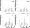 |
Fig. 2 Time sampling toward the 4 monitored targets in the Galactic spiral arms: average number of measurements per star and per week. |
3.1. EROS color–magnitude diagrams
The stars detected in EROS are statistically described by their color–magnitude diagrams given in Fig. 3 in the (IC,VJ) photometric system, hereafter simply noted (I,V).
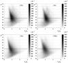 |
Fig. 3 Relative color–magnitude diagrams n(I,V − I) of the EROS catalogs toward the 4 directions toward the Galactic spiral arms. The gray scale gives the number density of stars per square degree, unit of magnitude, and unit of color index. |
The published EROS-CMDs provide for each catalog, labeled (C), the observed stellar density nC(I,V − I) per square degree, magnitude, and color index, as a function of I and V − I, sampled in 0.3 × 0.2 cells (Rahal et al. 2009a). When using these CMDs, one has to take into account the following uncertainties:
-
Each stellar number density nC(I,V − I) value is affected by a statistical uncertainty coming from the propagation of the Poissonian noise in the original EROS catalogs, as explained in the header of the published EROS-CMD (Rahal et al. 2009a).
-
Each nC(I,V − I) value is affected by a systematic uncertainty of ~5.3%, owing to the uncertainty on the size of the effective EROS field; this uncertainty is common to all catalogs.
-
Another systematic uncertainty is due to the residual 0.07 mag EROS calibration uncertainty (Blanc et al. 2004), which affects the attribution of a star to a given [ I,(V − I) ] cell. It has to be taken into account for each EROS color, and therefore induces a systematic uncertainty of [ 0.07,0.16 ] mag. in the [ I,V − I ] ≡ [ REROS,(BEROS − REROS) / 0.6 ] system.
To generate an “EROS-like” catalog from a model for comparison puroposes, one needs to use the efficiency of EROS to detect stars and the photometric uncertainties, both defined in the EROS photometric system [ REROS,BEROS ] ≡ [ I,I + 0.6(V − I) ]. The EROS stellar detection efficiency has been studied in (Rahal et al. 2009b), by comparing EROS data with HST data (HST 2002). Since we found that an object detected in BEROS is systematically detected in REROS, the EROS stellar detection efficiency can be parametrized as a function of the relative magnitude BEROS only (Fig. 4).
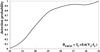 |
Fig. 4 Star detection probability in EROS vs. the relative magnitude BEROS = I + 0.6(V − I). |
The EROS photometric errors on the magnitudes and colors are parametrized as ![\begin{eqnarray} \delta I&=&\sqrt{0.1^2+ \left[\frac{2.5}{\ln 10}\right]^2\left[\frac{\sigma_{\Phi}}{\Phi}\right]_{R_{\rm EROS}}^2\frac{1}{N_{\rm meas}}}, \label{photoerr} \\ \label{photoerrcol} \delta(V-I)&= \sqrt{0.1^2\!+\!\left[\frac{1}{0.6}\frac{2.5}{\ln 10}\right]^2\left(\left[\frac{\sigma_{\Phi}}{\Phi}\right]_{R_{\rm EROS}}^2\!\!\! +\!\left[\frac{\sigma_{\Phi}}{\Phi}\right]_{B_{\rm EROS}}^2 \right)\frac{1}{N_{\rm meas}}}, \nonumber \end{eqnarray}](/articles/aa/full_html/2017/08/aa30488-17/aa30488-17-eq55.png) (8)where the 0.1 constant term (dominant for stars brighter than ~18) is a residual uncertainty, as estimated from EROS calibration studies using DENIS catalog data (Epchtein et al. 1999)1, [σΦ/ Φ] is the relative image-to-image dispersion of the successive flux measurements given by Fig. 5, and Nmeas is the number of observations (exposures) used to estimate the mean flux of a star, i.e., 268 toward β Sct, 277 toward γ Sct, 454 toward γ Nor and 375 toward θ Mus.
(8)where the 0.1 constant term (dominant for stars brighter than ~18) is a residual uncertainty, as estimated from EROS calibration studies using DENIS catalog data (Epchtein et al. 1999)1, [σΦ/ Φ] is the relative image-to-image dispersion of the successive flux measurements given by Fig. 5, and Nmeas is the number of observations (exposures) used to estimate the mean flux of a star, i.e., 268 toward β Sct, 277 toward γ Sct, 454 toward γ Nor and 375 toward θ Mus.
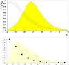 |
Fig. 5 Photometric point-to-point precision along the EROS light-curves vs. REROS = I (upper) and BEROS (lower). Vertical bars in I show the dispersion of this precision in the EROS catalog. The histograms show the magnitude distribution of the full EROS spiral arm catalog (all directions). |
Table 1 summarizes some of the key numbers regarding the color–magnitude statistical data. When comparing the data with simulations, we focus on the stars brighter than I = 18.4, the most reliable part of the EROS-CMD, with the highest and best controlled stellar detection efficiency.
3.2. Microlensing results
Data and results toward the 4 regions monitored in the EROS spiral arms program.
Table 1 provides the microlensing results from EROS (Rahal et al. 2009b). The σtE values differ from the values published in Table 3 from (Rahal et al. 2009b) because they were biased, since we assumed large statistics for their estimates. To properly take into account the statistical fluctuations on small numbers, we therefore re-estimated σtE from expression, 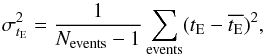 (9)where Nevents is the number of microlensing events toward the target.
The average microlensing detection efficiency of the EROS survey was estimated in Rahal et al. (2009b); it is defined as the ratio of events satisfying the EROS selection cuts to the theoretical number of events with an impact parameter u0< 1, and was found to be almost independent of the target, since the time samplings were very similar. Figure 6 shows this efficiency as a function of the Einstein duration of the events tE.
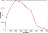 |
Fig. 6 Microlensing detection efficiency of the EROS survey toward the Galactic spiral arms, as a function of the event characteristic duration tE. |
4. How to synthesize an EROS-like color–magnitude diagram
We now compare the data with realistic simulations. In this section we describe how our modeling takes into account all the known observational constraints and discuss how to handle the specific difficulties of this kind of analysis.
We generated apparent color–magnitude diagrams based on the following hypotheses and ingredients from direct observations:
-
The Hipparcos catalog (ESA 1997; Turon etal. 1995) provides the magnitudes and colors of118218 local stars. We assume that the local population isrepresentative of the entire Galactic disk stellar population. Thishypothesis is certainly justified for the disk stars. The central barstellar population is redder, but the EROS observations we areconsidering here do not point toward its center.
-
A random magnitude shift is induced to take into account observational limitations, such as blending and uncertainties, from the Hipparcos and EROS data.
-
The spatial mass density distribution results from the addition of the contributions of thin and thick disks and of the bar modeled according to Binney & Tremaine (1987) and Dwek et al. (1995) or to the Besançon model (Robin et al. 2003).
-
The light propagation is affected by Galactic extinction in I and reddening in V − I, obtained from a 3D table of KS extinctions kindly provided by (Marshall, priv. com. 2015).
4.1. Producing a CMD from the local HIPPARCOS catalog
We present in Appendix A our procedure to obtain a debiased CMD in the (I,V) color system within the domain 0 <MV< 8 from the Hipparcos catalog. This debiased catalog is described by the distribution n(M), where M represents the absolute magnitude and color “vector” of a given stellar type. We established in Appendix A that the numerical contribution of stars brighter than MV = 0 is negligible in a deep Galactic image. In our case, given our limiting magnitude, we can also neglect the contribution of stars fainter than MV = 8.
Assuming that the stellar composition is constant along the line of sight, stars of any given type are distributed along the line proportionally to the total mass density ρ. The number of stars expected per square degree (Ω(1° × 1°) = 3.046 × 10⁻⁴ sr) in the EROS catalog is then the integral along the line of sight 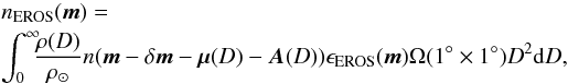 (10)where
-
D is the distance to the star along the line of sight,
-
μ(D) the corresponding distance modulus (independent on the color),
-
A(D) is the interstellar extinction vector (one component per filter)
-
δm is a random shift of m that takes into account blending (see Sect. 4.3.1) and uncertainties from Hipparcos parallax and EROS photometry; Hipparcos stellar absolute I magnitudes are randomly shifted according to a Gaussian distribution of dispersion
![\begin{equation} \epsilon_I=\sqrt{\left[5 \log e \times\frac{\delta\pi}{\pi}\right]^2+(\delta I)^2}, \label{errorI} \end{equation}](/articles/aa/full_html/2017/08/aa30488-17/aa30488-17-eq112.png) (11)where π and δπ are the Hipparcos parallax and associated error, and δI is the estimated EROS photometric uncertainty from expression (8). The colors V − I are similarly randomly shifted with the dispersion
(11)where π and δπ are the Hipparcos parallax and associated error, and δI is the estimated EROS photometric uncertainty from expression (8). The colors V − I are similarly randomly shifted with the dispersion 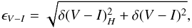 (12)where δ(V − I)H is the uncertainty on the color from the Hipparcos catalog and δ(V − I) is given by Eq. (8).
 -
ϵEROS(m) is the probability to detect a star with apparent magnitudes m in the EROS catalog (see Fig. 4). Here this probability is a function of BEROS only, which is related to the absolute magnitudes and to the distance D as follows:
 (13)
(13)
4.2. Mass density distributions
In this section, we describe two mass distribution models used to scale the local densities of lenses and sources along the line of sight. We note the different status of the thick disk: it is considered hypothetical within the framework of the first model (so-called simple) since it is a pure hidden matter contribution; on the other hand, it is considered as one of the components within the framework of the second model (Besançon).
4.2.1. Simple tunable Galactic model
In this model, which is slightly modified (updated) from the so-called model1 we used in Rahal et al. (2009b), the mass density of the Galaxy is described with a thin disk and a central bar structure. The disk is modeled by a double exponential density in galactocentric cylindrical coordinates 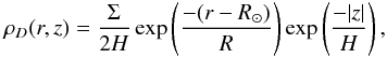 (14)where Σ = 50 M⊙ pc-2 is the column density of the disk at the solar radial position R⊙ = 8.3 kpc (Brunthaler et al. 2010), H = 0.325 kpc is the height scale, and R = 3.5 kpc is the radial length scale of the disk. The position of the Sun with respect to the symmetry plane of the disk is z⊙ = 26 pc ± 3 pc (Majaess et al. 2009). The bar is described in a Cartesian frame positioned at the Galactic center with the major axis X tilted by Φ = 13° (Robin et al. 2012) with respect to the Galactic center-Sun line, i.e.,
 ![\begin{equation} \rho_{B} = \frac{M_{B}}{6.57 \pi abc} e^{-r^{2}/2} , r^{4} = \left[ \left( \frac{X}{a} \right)^{2} + \left( \frac{Y}{b} \right)^{2} \right]^{2} + \frac{Z^{4}}{c^{4}} , \end{equation}](/articles/aa/full_html/2017/08/aa30488-17/aa30488-17-eq129.png) (15)where MB = 1.7 × 10¹⁰M⊙ is the bar mass, and a = 1.49 kpc, b = 0.58 kpc, and c = 0.40 kpc are the scale length factors.
(15)where MB = 1.7 × 10¹⁰M⊙ is the bar mass, and a = 1.49 kpc, b = 0.58 kpc, and c = 0.40 kpc are the scale length factors.
There has been some controversy about the bar inclination Φ; in particular, the EROS collaboration (Hamadache et al. 2006) published an erroneously high value (Φ = 49° ± 8°) deduced from the variation of the mean distance to the red giant stars with the Galactic longitude. This mean distance was confused with the distance to the bar major axis, but this view is only correct for a zero width bar. As a consequence, the value of Φ was strongly overestimated, since as soon as the bar is elliptic, the barycenters of the stars along the line of sight do not coincide with the bar main axis (López-Corredoira et al. 2007). Moreover, this difference between the barycenter line and the main axis increases when Φ decreases and when the width of the bar increases. Correcting this wrong view, we checked that the EROS red giant clump distance measurements are in fact compatible with the low values of Φ recently published (Robin et al. 2012; Wegg et al. 2015), as discussed in the following sections.
The hypothetical thick disk is also considered in our model, and we fit its fractional contribution fthick to the Galactic structure (fthick = 1 would correspond to fully baryonic Galactic hidden matter). This disk is modeled as the thin disk (Eq. (14)), with Σthick = 35 M⊙ pc-2, Hthick = 1.0 kpc, and Rthick = 3.5 kpc.
The IMF of the stellar population is taken from Chabrier (2004) (Eq. (A.9)). We already mentioned that we expect the microlensing duration to be especially sensitive to the low-mass side of the IMF of the lens population. We therefore define a tunable function for the low-mass side IMF (m ≤ M⊙), by introducing a parameter m0 (with value m0 = 0.2 M⊙ for the regular Chabrier IMF): ![\begin{equation} \xi(\log m/\Msol)= 0.093\times \exp\left[\frac{-(\log m/m_0)^2}{2\times (0.55)^2}\right],\,{\rm for}\,m\le \Msol \label{massfunction} \end{equation}](/articles/aa/full_html/2017/08/aa30488-17/aa30488-17-eq144.png) (16)and we fit this parameter to our microlensing duration data in Sect. 6.
(16)and we fit this parameter to our microlensing duration data in Sect. 6.
We use the following kinematical parameters:
-
The radial (axis pointing toward the Galactic center), tan-gential and perpendicular solar motions with respect to thedisk are taken from (Brunthaler et al. 2010),
 (17)We found that the microlensing duration distribution obtained in our simulation is almost insensitive to the exact values of these parameters.
 -
The global rotation of the disk is given as a function of the galactocentric distance by
![\begin{equation} V_{\rm rot}(r) = V_{\rm rot,\odot} \times \left[ 1.00767 \left( \frac{r}{R_{\odot}} \right)^{0.0394} + 0.00712 \right] , \end{equation}](/articles/aa/full_html/2017/08/aa30488-17/aa30488-17-eq146.png) (18)where r is the projected radius (cylindrical coordinates) and Vrot, ⊙ = 239 ± 7 km s-1 (Brunthaler et al. 2010).
(18)where r is the projected radius (cylindrical coordinates) and Vrot, ⊙ = 239 ± 7 km s-1 (Brunthaler et al. 2010). -
The peculiar velocity of the (thin or thick) disk stars is described by an anisotropic Gaussian distribution with the following radial, tangential, and perpendicular velocity dispersions (Pasetto et al. 2012a,b):
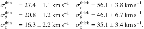 (19)We also found that the microlensing duration distribution is insensitive to the exact values of these parameters.
 -
The velocity distribution of the bar stars is given by the combination of a global rotation (Fux 1999; Portail et al. 2017)
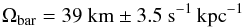 (20)with a Gaussian isotropic velocity dispersion distribution characterized by σbar ~ 110 km s-1. We found that the mean duration of microlensing events toward γ Sct, which is the only line of sight crossing the bar, is almost insensitive to Ωbar, mainly because the global rotation velocity is almost tangent to this line of sight.
4.2.2. Besançon Galactic model
In this model (Robin et al. 2003, with updated parameters from Robin et al. 2012), the distribution of the matter in the Galaxy is described by the superposition of eight thin disk structures with different ages, a thick disk component, and a central (old) bar structure made of two components (Robin et al. 2012). We considered the updated model from (Robin et al. 2012) that appears to be specifically adapted to the Galactic plane, and chose the fitted parameters associated with a two ellipsoid bar (Freundenreich (S) plus exponential (E) shapes). All the parameters from this model can be found in the Appendix B, to enable any useful comparison with our simple model.
4.2.3. From the local CMD and mass density to the stellar distribution
The mass densities are then converted into stellar number densities and distributed according to our debiased Hipparcos-CMD (Sect. 4.1). The number density of stars scales with the stellar mass density, such that the total number density of stars within 0 <MV< 8 equals the total mass density within the corresponding mass interval [ 0.65,2.8 ] M⊙, divided by the mean stellar mass in this interval, as computed from the IMF. We finally take into account the fact that ~2:3 of those stars are in binary systems, as discussed in Sect. A.2. This 2:3 poorly known factor and the exact mass to stellar number ratio can both be absorbed in a global renormalization factor, and our simulated catalog has been tuned to precisely reproduce the local (debiased) observed Hipparcos-CMD.
We have now in hand the full description of stellar number densities according to the mass densities and the debiased Hipparcos-CMD, which is our initial ingredient to simulate EROS-like CMDs.
4.3. Extinction
We now have to consider the absorption model to simulate the effects of distance and reddening of the sources in expressions (10) and (13).
After generating the position and type of a star, we estimate the extinction due to dust along the line of sight using the table provided by (Marshall, priv. com. 2015). This 3D table provides AK, the extinction in KS in the (b,l) = ( ± 10°, ± 100°) domain, up to ~15 kpc, with 0.1° angular resolution and 0.1 kpc distance resolution. We use the following relations to transpose the AK into I and V passbands  (21)We compared the extinctions from this table with the 2D table of (Schlegel et al. 1998) (through extrapolation at infinite distance), which is notoriously imprecise toward the Galactic plane, and with the calculator of (Schlafly & Finkbeiner 2011)2. We found that up to ~5 kpc, the extinctions in I from Schlafly & Finkbeiner (2011) are compatible with the Marshall table, although systematically lower. At larger distances, the estimates depart from each other, and extrapolations at large distance from Marshall table are much larger than estimates from both Schlegel et al. (1998) and Schlafly & Finkbeiner (2011). Nevertheless, as discussed in Sect. 5.1, we found it necessary to correct the extinctions of the Marshall table for systematic and statistical uncertainties, to get synthetic CMDs of I< 18.4 stars that correctly match the observed CMDs (compare Figs. 7 with 10); indeed, because of the large multiplicative factor relating AV and AI to AK, a small error on AK has a very significant impact on the apparent position of a star in our CMD. Fig. 12 shows the average extinctions in V along the lines of sights as a function of the distance to the source, after tuning the model parameters according to our fitting procedure.
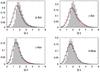 |
Fig. 7 The V − I observed (gray histograms) and the simulated distributions (simple model in black, Besançon model in red) for the bright stars (with I< 18.4), using the Marshall table without systematic/statistical uncertainties (to be compared with Fig. 10, bottom). |
4.3.1. Blending
We know from the comparison of the EROS images with the HST images (Rahal et al. 2009b) that ~60% of the I< 16 objects and ~70% of the I> 16 objects detected by EROS are blends. This blending effect is different than the binary blend mentioned at the end of Appendix A. This effect, due to the EROS low separation power, is accounted for by randomly decreasing the magnitudes of 60% of the faint stars (resp. 70% of the bright) according to a Gaussian distribution centered on − 0.07, with σ = 0.25 (resp. 0.13), troncated at zero.
In principle, blending also contributes to reduce the number of detected objects with respect to the predictions based on the Hipparcos catalog. As for the binary blend, this effect can be absorbed in a global renormalization factor.
5. Comparing the EROS observations with simulated populations and microlensing expectations
Our aim is now to tune and compare the Galactic models with the observations toward the four Galactic disk lines of sight (characterized by the corresponding EROS catalogs noted C). We use all the available observables for this purpose as follows:
-
The four color–magnitude distributions (CMD) of stars brighterthan I = 18.4, which is the most reliable part of the EROS-CMD. The observable variables we consider are derived from the projected magnitude and color distributions: the total stellar densities ρ∗3, and the first moments
 and σV − I of the V − I distribution4.
 -
The measured optical depths τ(C) (Rahal et al. 2009b) toward the four catalogs C (Table 1).
-
The measured means
 (Rahal et al. 2009b) (Table 1). The poor available statistics convinced us not to use the σtE parameter in our fitting procedure, since it is affected by such a large uncertainty that it is essentially not constraining.
For quantitative statistical comparisons based on χ2 studies, we need good control of the uncertainties on these observables. The τ and  uncertainties are provided in Rahal et al. (2009b). Table 1 summarizes the numerical data toward the EROS monitored populations that we use for the comparison with a simulation (apart σtE).
5.1. Simulation of the CMDs
All the relevant information is already given in Sect. 4. Here, we briefly summarize the different stages to simulate EROS CMDs from various models or parameters.
The stellar absolute magnitudes and colors are first randomly chosen according to the Hipparcos unbiased color–magnitude density diagram of stars with 0 <MV< 8 (Fig. A.4 bottom). Generated magnitudes are then shifted to take into account the blending described in Sect. 4.3.1, as well as the Hipparcos parallax uncertainties and EROS photometric uncertainties (Eqs. (11) and (12)).
To estimate the integral in expression (10), we generate the distance distributions of stars according to the mass density distributions of each Galactic structure (bar, thin disk, or thick disk). The EROS stellar apparent magnitudes and colors are estimated from the absolute magnitudes, the distances, and take into account the absorptions tabulated (in KS) at the position randomly chosen within the EROS fields (see Sect. 4.3). After this stage, we obtain the apparent color–magnitude distribution of the stars before detection. Finally, the contribution of each generated star is weighted by the EROS stellar detection efficiency ϵEROS(m), which is parametrized as a function of BEROS (Fig. 4).
As mentioned in Sect. 4.3, to successfully fit the CMDs we had to introduce the hypothesis of a systematic uncertainty on KS changing with the catalog, ΔAK(C), and a random uncertainty with constant width ϵAK, within the tabulated data. Since the table does not provide uncertainties, we used this hypothesis as the simpliest way to make our simulation compatible with the observations (Robin, priv. comm.). Then the ΔAK(C) and ϵAK parameters were tuned together with the Galactic parameters to obtain synthetic CMDs that fit the observed CMDs (see below).
5.2. Simulation of microlensing
The previous procedure, based on the synthesis of the color–magnitude diagrams, allows us to simulate the EROS catalogs of sources. To simulate the microlensing process for these catalogs, we also need to synthesize the population of lenses, containing all massive objects regardless of their visibility. The local lens density population is therefore simulated with the appropriate IMF (depending on the Galactic structure and on the model) scaled with the local mass density. The transverse velocity distribution needed to simulate the microlensing event durations is obtained from the combination of the velocity distributions from the disk(s) and the bar, according to their respective local mass contributions. Finally, we take into account the impact of the time sampling by simulating the microlensing detection efficiency according to Fig. 6.
6. Fitting procedure
Our simulation program allows us to produce the CMDs and microlensing distributions toward our 4 catalogs labeled (C), with any choice of Galactic parameters. We detail below the procedure developed for our simple tunable model, which we also used to probe the Besançon model (with no tuned parameter other than the systematic uncertainties of the interstellar absorptions).
6.1. Fit and tuning of the simple model
We examined the following 16 observables (4 per target C) ρ∗(C),  , τ(C), and as a function of the following parameters, around their nominal values: ϵAK, the random uncertainty on the extinctions AK provided by the table from Marshall et al. (2006) for each generated stellar position; ΔAK(C), the systematic uncertainty on AK(C), depending on the catalog(C); the Galactic bar inclination Φ (nominal value Φ = 13°); and the (hypothetic) thick disk contribution, which is parametrized by the fraction fthick of the thick disk considered in (Rahal et al. 2009b). This contribution is modeled like the thin disk (see Eq. (14)), with Σthick = fthick × 35 M⊙ pc-2, Hthick = 1.0 kpc, Rthick = 3.5 kpc, and velocity dispersions given by Eq. (19).
To benefit from the exclusive time information provided by the microlensing data, we also considered some specific parameters that are expected to impact the microlensing optical durations. First, the low-mass part of the IMF, which we generalized from Chabrier (2004) through parameter m0 (nominal value m0 = 0.2) (Sect. 4.2.1). Second, we explored the sensitivity to the peculiar velocities of the microlensing actors through a scaling of the velocity dispersions reported in expression (19). We found that our simulation is insensitive to such a scaling, therefore confirming that orbital velocities dominate the relative transverse motions. Third, for completeness, we also tested the sensitivity of with the global rotation of the bar (Eq. 20) and found almost no sensitivity; this is mainly because the bar rotation is almost tangent to the line of sight of γ Sct, which is the only line of sight that crosses the bar structure.
6.1.1. Sensitivity of the observables with respect to the Galactic parameters
We used our simulation to establish the sensitivity of the observables with the variations of the different parameters, and we made the following observations.
We find that only the simulated observables from the low longitude fields (β Sct and γ Sct) are sensitive to the variations of Φ, when we test for very large changes, but they are insensitive to few degree variations around the nominal value Φ = 13°. As a consequence, we exclude Φ from our fit.
At first order, the absorption random shift dispersion ϵAK, with respect to the tabulated values, is assumed to be the same for all fields, and the widths of the four color distributions σV − I(C) are found to be disconnected from the other observables and parameters. We therefore directly fit ϵAK by minimizing the differences between  and the width combination
  , where the 3.85 factor comes from the relation AV − I = 3.85 × AK (see Sect. 4.3), and the
  values are obtained with a simulation that assumes ϵAK = 0. The value that minimizes the sum on (C) is ϵAK = 0.085, which we assume to be independent of the catalog C. We use this value in the subsequent simulations.
The Chabrier-like IMF parameter m0 and the observables are also disconnected from the other observables and parameters. We therefore make a separate (sub-)fit for these parameters, by minimizing 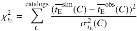 (22)with respect to m0, where the suffixes sim and obs refer to the simulated and observed catalogs.
The observables ρ∗(C), , and the microlensing optical depths τ(C) (12 observables) depend only on fthick and on the systematics ΔAK(C) (5 parameters). We performed a combined fit by minimizing the sum of  ,
,  and
and  , which is defined similar to
  , but since we have to take into account common systematics, some of the covariant matrices are not diagonal.
In our minimization procedure, we used the first order developement of the observables as functions of the parameters to be fitted, from the derivatives computed with our simulation. This allowed us to perform the fit with acceptable computing time, considering the very long runs needed for each model configuration.
6.1.2. Systematic and statistical uncertainties
We have carefully established the budget error for each observable as follows.
For the ρ∗(C) budget error, we have to take into account the uncertainty of ~5.3% on the size of the effective EROS field and the consequences of the 0.07 magnitude EROS calibration uncertainty. The impact of this calibration uncertainty on ρ∗(C) has been estimated from the published EROS-CMD tables, by changing the position of the I< 18.4 mag cut by the 0.07 systematics. We found that the uncertainty on ρ∗(C) due to this calibration error is ~5%. The final systematics results from the quadratic addition of both uncertainties (7.3%) and since it is a multiplicative systematics, it has to be considered as an uncertainty on a global normalization α; we therefore use a standard procedure to include the extra parameter α and fit the product  with
with  . We adopt 15% as the statistical uncertainty on ρ∗(C), which is dominated by residual uncertainties from the absorption model and blending effects.
For , we have to account for the systematics due to calibration uncertainties on both REROS and BEROS, thus giving a global systematics of 0.16 mag. In the covariance matrix associated with the fit minimization, this additive systematics, which is common to the four directions, contributes as a full matrix, to be added to the usual diagonal matrix built from the residual statistical uncertainty that is estimated to be 0.15 mag.
Statistical uncertainties from the EROS-CMD Poissonian fluctuation propagation are estimated as explained in the header of the published EROS-CMD (Rahal et al. 2009a). Considering the large statistics available in the EROS database, we can neglect the uncertainties due to the Poissonian fluctuations of the number of stars in the original EROS histogram used to produce the CMDs.
As a conclusion, the uncertainties on ρ∗(C), and σV − I(C) are dominated by the impact of the calibration uncertainties and the residual uncertainties from blending and absorption effects discussed above. The values used for the fit are summarized in Table 2.
6.1.3. Results from the fit
We remind that the fit is done with the best value for the random uncertainty on the tabulated absorptions AK: ϵAK = 0.085. The best fit is obtained with the following parameters.
First, regarding absorption systematics, we find ΔAK(βSct) = 0.09 mag, ΔAK(γSct) = 0.04 mag, ΔAK(γNor) = 0.11 mag, and ΔAK(θMus) = − 0.01 mag.
Second, regarding the fraction of the thick disk, we find fthick = 0.05 ± 0.6. This result does not differ from zero, showing that there is no need for an additional baryonic contribution to the thin disk within the framework of our simple model. We also tested the option of a non-luminous thick disk (made of compact unseen objects), assuming no contribution to the CMD (therefore only impacting the optical depths); we found finvisible thick = 0.5 ± 0.9, which is again not significantly different than zero. From this estimate, we can conclude that the total mass of an invisible thick disk is smaller than 7 × 10¹⁰M⊙ at 95%CL.
Third, regarding the IMF, we find m0 = 0.51 ± 0.25 M⊙, which is somewhat significantly different than the 0.2 nominal value of the local Chabrier IMF (Chabrier 2004). Our observations are therefore significantly sensitive to the low-mass side of the lens IMF. This sensitivity belongs to a non-local IMF, since it concerns only the lenses and not the solar neighborhood. Figure 8 shows both IMFs (the local and best fitted lens-IMF).
For this global fit of the CMDs, optical depths and microlensing durations, we find χ2 = 6.5 for 10 degrees of freedom with a fair repartition between the different types of observables (ρ∗, , τ and tE).
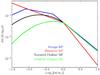 |
Fig. 8 Different mass functions considered in this paper: Standard Chabrier (black) corresponds to the local regular Chabrier IMF (Eq. (A.9) with m0 = 0.2 M⊙); the modified Chabrier (m0 = 0.51 M⊙, in green) gives the best fit for the lens IMF from our simple model. |
We exchanged in our simple model the Chabrier IMF for the Kroupa IMF (Kroupa 2001). The only consequence to this exchange was a significant decrease in the values, as expected from the larger contribution of low-mass objects (see Fig. 8 and Table 2). This degrades the fit by 7.4 units, showing that the Kroupa IMF is strongly disfavored by our data.
It is clear that a larger statistics of microlensing events toward the spiral arms would have the capability to better constrain the thick disk component and the lens-IMF.
Table 2 summarizes the best fit results for our simple model compared with previous simulations (model 1) considered in Rahal et al. (2009b), differing mainly through the extinction description.
Best fit results on the observables toward the 4 regions monitored in the EROS spiral arms program, compared with previous simulations (model 1) and observations published in Rahal et al. (2009b).
Figure 9 shows the mass density along the line of sight of γSct resulting from our simple fitted model.
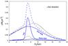 |
Fig. 9 Mass-density along the line of sight of γSct from the various Galactic structures (disks and bar), as a function of the distance from the Sun for our nominal simple model (thin black lines) and the Besançon model (thick blue lines). The total densities are shown with dashed lines. |
6.2. Besançon model: tuning the extinctions
In this section, our purpose is to test the agreement of the Besançon model with the EROS microlensing results. We used almost the same procedure as above, but fitting only the uncertainties on the K extinctions. The best fit is obtained for ϵAK = 0.10, ΔAK(βSct) = 0.14 mag, ΔAK(γSct) = 0.13 mag, ΔAK(γNor) = 0.15 mag, and ΔAK(θMus) = 0.04 mag. The global fit has a χ2 = 8.2 for 12 d.o.f, with specific contributions of  ,
,  ,
,  , and
, and  .
.
Not surprisingly, the values of and are worse than those of our simple model, since no parameters are fitted for the thick disk and the IMF, but the fit is globally satisfying (see Table 2 for the summary of the fitted parameters and observables). Figure 9 shows the mass density along the line of sight of γSct from the Galactic structures of the Besançon model (in blue), resulting from the best fitted extinction.
As for the previous simple model, we also tested the hypothesis of an invisible extra contribution to the thick disk for this model; we find that the best fitted value for such a thick disk favors an added contribution of 2.5 ± 4.7 times the modeled thick disk (χ2 = 8.0 per 11 d.o.f.). Again, there is no significant indication of the need for such an invisible contribution and the upper limit of a Besançon-like thick disk (somewhat thinner than in our simple model) is ~5 × 10¹⁰M⊙ at 95%CL.
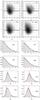 |
Fig. 10 Simulated CMDs toward the 4 monitored directions (top) with the magnitude (middle) and color (bottom) projections for the stars brighter than I = 18.4, expressed in million of stars per square degree per magnitude. Results from our simple model are plotted with black lines and results from the Besançon model with red lines; the distributions of the EROS observed populations of bright stars (I< 18.4) are superimposed on the projections as light gray histograms. |
7. Discussion
As a preliminary to the discussion, we recall here some of the hypotheses used throughout this paper: First, we assume the disk to have the same CMD as around the sun; then we rely on the extrapolation of the extinction map obtained in K band to I and V bands, and assume reasonable systematic uncertainties on this map.
7.1. Comparison with previous results and robustness
Figure 10 (to be compared with Fig. 3) shows that our best fitted models are able to reproduce satisfactorily the observed CMDs of the (I< 18.4) stars. Table 2 shows that the model we used previously (model 1) was also satisfactory. We tested the robustness of our results by changing some of the uncertainties (systematics and statistics) with unsignificant variations of the best fitted numbers.
Our model now incorporates enough details to allow one to use the CMD as an observable to be fitted. As a consequence, the main impact of this type of study, apart from constraining the parameters fthick (for our simple model) and m0, is to extract information on the underlying stellar populations of sources and lenses.
7.2. Lens and source populations
Figure 11 shows the fast variation of the simulated optical depth along the line of sight with the distance for the four studied directions and for both models considered in this paper.
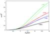 |
Fig. 11 Simulated optical depths toward the 4 monitored directions, as a function of the source distance, for our nominal simple model (thin lines) and the Besançon model (thick lines). |
This fast variation of the optical depth with the distance shows that the notion of catalog optical depth is crucial when dealing with sources distributed along a line of sight. This notion is not relevant when considering well-defined distance targets such as LMC, SMC, and M31; when considering only bright sources toward the Galactic Center, it is estimated that the relative uncertainty on the bright source’s positions is less than 10% (Paczyński & Stanek 1998) and it is still possible to ignore the spread of the sources and to use the classical concept of optical depth up to a given distance for the whole catalog. Previous studies concerning the Galactic spiral arms (Derue et al. 1999; Derue et al. 2001) performed a simplified analysis, by assuming all sources to be at 7 Kpc to compare the observed optical depth with simple models, but Rahal et al. (2009b) started to draw attention to the impact of the source distance spread. Now it is clear that precise studies in the Galactic plane are needed to know the distance distribution of the monitored catalog. Figure 12 shows the expected distance distributions of the lenses and sources in the EROS microlensing events obtained from our simulation (taking into account the EROS efficiencies). Again, the source distance distribution illustrates the relevance of the concept of optical depth toward a population in contrast with the optical depth up to a given distance.
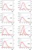 |
Fig. 12 Expected normalized distributions of the distances for the lensed sources – when taking into account the EROS microlensing detection efficiencies – (thin lines) and of the lenses (thick lines) from the simulation of our simple model (upper) and the Besançon model (lower). The sparsely-populated distributions around 4 kpc (for β Sct and γ Sct) correspond to the contribution of the bar objects. The dashed curves show, as a function of the distance, the average extinctions of the stars in the simulated EROS-like catalog (in V magnitude, on the right scale). It is strongly biased in favor of small extinctions mainly due to the magnitude selection I< 18.4. |
7.3. Constraining the Galactic model: the specific contribution of microlensing data
The good agreement of our Galactic models with the data shows that there is no need for other or more ingredients. The Besançon model predicts relatively small optical depths, and this observation is in agreement with the deficit of optical depth toward the inner bulge directions noticed by MOA-II (Awiphan et al. 2016), even if this is not very significant from our reduced statistics.
We also used our simulation to measure the domain of Galactic parameters that is compatible with our observations. We focused on parameters that are expected to impact the microlensing optical depths or durations, i.e., the bar inclination Φ (nominal value Φ = 13°); the thick disk contribution, parametrized by the fraction fthick, either visible (for the simple model) or invisible (for both models); the disk kinematics for which we explored our sensitivity through the scaling of the velocity dispersions (in expression (19)); and the IMF parameter m0, as defined in Sect. 6.
The impact of the Galactic bar is illustrated in Fig. 12, where it is clearly visible that it mainly intercepts the γ Sct line of sight; in the present case, owing to low statistics, our data can only distinguish between a small or a large bar angle, but cannot refine its current estimate. Nevertheless, it is clear that systematic microlensing study at relatively small Galactic longitude is a promising technique to precisely measure the bar inclination.
We show that there is no significant need for an extra thick disk component (visible or invisible); otherwise, from our data alone there are not enough constraints to exclude its existence and only a 95% CL upper limit on its total mass could be inferred (~7 × 10¹⁰M⊙ for the simple-model thick disk, ~5 × 10¹⁰M⊙ for an extra invisible component in the Besançon-model thick disk).
We found that we cannot constrain the velocity dispersion ellipsoids of the microlensing actors, since the transverse velocities involved in the microlensing durations are dominated by the orbital velocities.
Interestingly, we show that microlensing durations can constrain the low-mass end of the mass function (see Fig. 13), and more importantly, it can provide such constraints for non-local stellar populations (the disk lens population); this is in contrast with the other techniques, which can only measure the mass function around the Sun.
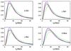 |
Fig. 13 Einstein duration tE distribution of the microlensing events expected by assuming 4 different IMFs: the standard Chabrier (black), the Besançon model (red), the modified Chabrier (with m0 = 0.57, green), and the Kroupa IMF (blue). |
The best fitted value we obtain for our parametrized Chabrier-type IMF of the lens population of the disk is m0 = 0.51 ± 0.25, which is in relative disagreement (by one standard deviation) with the parameter of the local mass function (m0 = 0.2) of the Chabrier model. This discrepancy originates in the longer mean durations of the observed events compared with the simulation based on the local IMF. The microlensing technique seems to be significantly sensitive to the IMF low-mass end.
We find that the Kroupa IMF does not correctly reproduce the mean durations of our microlensing events, because of the higher contribution of low-mass objects, inducing a deficit of predicted long duration events.
7.4. Limitations of this study
We have made a considerable effort to understand the CMDs and the microlensing data toward directions that have not been examined by other teams. For this reason, we note the limits we encountered during this study to avoid any missinterpretation. Knowledge of the absorption map was one of the most important limitations. Its precision and resolution within the studied fields are parameters that impact the CMD so strongly that we found it necessary to assume (reasonable) systematic and statistical dispersions to understand the observed densities of bright stars. The blending and the 2:3 estimated fraction of binary stars are also other sources of limitation for understanding the CMDs. All of these elements have fortunately a somewhat degenerated impact on the predicted stellar densities; without any correction to the extinctions, we found that the simulated CMDs had too many stars and were bluer than the data, which could be solved with a systematic extinction increase. These limitations impacts mainly the CMDs; the specific observables from microlensing (optical depth and durations) are mainly impacted through the distance distribution of the lenses.
8. Conclusions and perspectives
We have performed a complete simulation of the Galactic structure and the EROS acceptance, which is able to reproduce all the EROS exclusive observations toward the Galactic arms. In this view, we produced a debiased color–magnitude diagram from the Hipparcos catalog to feed our simulation with a realistic stellar population. This population was spatially distributed according to the Besançon Galactic model, and to a simple Galactic mass model including a thin disk and a central bar, with an adjustable thick disk contribution and IMF. Every simulated object was then considered as a potential gravitational lens as well as a potential source to gravitational lensing. Taking into account the dust extinction and EROS detection efficiencies, the observed color–magnitude diagrams and the microlensing optical depths and durations are correctly fitted with both our simple Galactic model (with no thick disk) and the Besançon model. We then used the simulation as a tool to obtain information on the configuration space of the microlensing actors (lens and source distance distributions). The large width found in this way for the source distance distribution validates the concept of “catalog optical depth” by contrast with the usual optical depth to a given distance. This concept is to be used as soon as the sources are widely distributed in distance. Finally, even with the small statistics of microlensing events, we were able to extract interesting constraints on the Galactic parameters – i.e., bar inclination confirmation, disk kinematics, mass function, and hidden matter – that have an impact on the microlensing distributions.
The running VISTA Variables in the Via Lactea (VVV) survey, which is monitoring stars within the Galactic plane in IR, is well suited to enlarge the field of view within the Galactic plane, by searching for microlensing in dusty regions. This survey should be able to better constrain the parameters mentioned above, with promising perpectives such as measuring the mass function in areas other than the solar neighborhood. The Large Synoptic Survey Telescope (LSST) will also have the capability to monitor a wide domain of the Galactic plane for microlensing, but only limited to the clear windows, free from large dust column densities.
Acknowledgments
This research was supported by the Perimeter Institute for Theoretical Physics and the John Templeton Foundation. Research at the Perimeter Institute was supported by the Government of Canada through Industry Canada and by the Province of Ontario through the Ministry of Economic Development and Innovation.
References
- Alcock, C., Akerlof, C. W., Allsman, R. A., et al. 1993, Nature, 365, 621 [NASA ADS] [CrossRef] [Google Scholar]
- Aubourg, É., Bareyre, P., Bréhin, S., et al. 1993, Nature, 365, 623 [NASA ADS] [CrossRef] [Google Scholar]
- Awiphan, S., Kerins, E., & Robin, A. 2016, MNRAS, 456, 1666 [NASA ADS] [CrossRef] [EDP Sciences] [Google Scholar]
- Binney S., & Tremaine S., 1987, Galactic Dynamics (Princeton, NJ: Princeton Univ. Press) [Google Scholar]
- Blanc, G., Afonso, C., Alard, C., et al. 2004, A&A, 423, 881 [NASA ADS] [CrossRef] [EDP Sciences] [Google Scholar]
- Brunthaler, A., Reid, M. J., Menten, K. M., et al., 2010, Astron. Nachr., 999, 789 [Google Scholar]
- Calchi Novati, S., Bozza, V., Bruni, I., et al. 2014, ApJ , 783, 86 [NASA ADS] [CrossRef] [Google Scholar]
- Chabrier, G. 2003, ApJ, 586, 133 [Google Scholar]
- Chabrier, G. 2004, the initial mass function: from Salpeter 1955 to 2005, eds. E. Corbelli, F. Palla, & H. Zinnecker, The Initial Mass Function 50 Years Later, 327, 10 [Google Scholar]
- Crotts, A. P. S., & Tomaney, A. B. 1996, ApJ, 473, L87 [NASA ADS] [CrossRef] [Google Scholar]
- Delfosse, X., Forveille, T., Ségranssan, D., et al. 2000, A&A, 364, 217 [Google Scholar]
- Derue, F., Afonso, C., Alard, C., et al. 1999, A&A, 351, 87 [Google Scholar]
- Derue, F., Afonso, C., Alard, C., et al. 2001, A&A, 373, 126 [NASA ADS] [CrossRef] [EDP Sciences] [Google Scholar]
- Dwek, E., Arendt, R. G., Hauser, M. G., et al. 1995, ApJ, 445, 716 [CrossRef] [Google Scholar]
- Epchtein, N., Deul, E., Derriere, S., et al. 1999, A&A, 349, 236 [NASA ADS] [Google Scholar]
- ESA 1997, The Hipparcos and Tycho Catalogues, ed. M. A. C. Perryman (Noordwijk: ESA), ESA SP, 1200 [Google Scholar]
- Fux, R. 1999, A&A, 345, 787 [NASA ADS] [Google Scholar]
- Gould, A. 1992, ApJ, 392, 442 [NASA ADS] [CrossRef] [EDP Sciences] [Google Scholar]
- Hamadache, C., Le Guillou, L., Tisserand, P., et al. 2006, A&A, 454, 185 [NASA ADS] [CrossRef] [EDP Sciences] [Google Scholar]
- HST 2002, HST archive, https://archive.stsci.edu/ [Google Scholar]
- Jahreiss, H., & Wielen, R. 1997, Hipparcos-Venice 97 (Noordwijk: ESA Publications), ESA Symp., 402, 675 [NASA ADS] [Google Scholar]
- Kroupa, P. 2001, MNRAS, 322, 231 [NASA ADS] [CrossRef] [Google Scholar]
- López-Corredoira, M., Cabrera-Lavers, A., Mahoney, T. J., et al. 2007, AJ, 133, 154 [NASA ADS] [CrossRef] [Google Scholar]
- Mao, S., & Stefano, R. D. 1995, ApJ, 440, 22 [NASA ADS] [CrossRef] [Google Scholar]
- Majaess D. J., Turner D. G., & Lane D. J. 2009, MNRAS, 398, 263 [NASA ADS] [CrossRef] [Google Scholar]
- Marshall, D. J., Robin, A. C., Reylé, C., et al. 2006, A&A, 453, 635 [NASA ADS] [CrossRef] [EDP Sciences] [Google Scholar]
- Moniez, M. 2010, Gen. Relativity Gravitation, 42, 2047 [NASA ADS] [CrossRef] [Google Scholar]
- Paczyński, B. 1986, ApJ, 304, 1 [NASA ADS] [CrossRef] [Google Scholar]
- Paczyński, B., & Stanek, K. Z. 1998, ApJ, 494, L219 [NASA ADS] [CrossRef] [Google Scholar]
- Pasetto, S., Grebel, E. K., Zwitter, T., et al., 2012a, A&A, 547, A70 [NASA ADS] [CrossRef] [EDP Sciences] [Google Scholar]
- Pasetto, S., Grebel, E. K., Zwitter, T., et al., 2012b, A&A, 547, A71 [NASA ADS] [CrossRef] [EDP Sciences] [Google Scholar]
- Popowski, P., Griest, K., Thomas, C. L., et al. 2005, ApJ, 631, 879 [NASA ADS] [CrossRef] [Google Scholar]
- Portail, M., Gerhard, O., Wegg, C., & Ness, M. 2017, MNRAS, 465, 1621 [NASA ADS] [CrossRef] [Google Scholar]
- Rahal, Y. R., Afonso, C., Albert, J.-N., et al. 2009a, Vizier Online Data Catalog: J/A+A/500/1027 [Google Scholar]
- Rahal, Y. R., Afonso, C., Albert, J.-N., et al. 2009b, A&A, 500, 1027 [NASA ADS] [CrossRef] [EDP Sciences] [Google Scholar]
- Rahvar S. 2015, Int. J. Mod. Phys. D, 24, 1530020 [NASA ADS] [CrossRef] [Google Scholar]
- Robin, A. C., Reylé, C., Derrière, S., & Picaud, S. 2003, A&A, 409, 523 [NASA ADS] [CrossRef] [EDP Sciences] [Google Scholar]
- Robin, A. C., Marshall, D. J., Schultheis, M., & Reylé, C. 2012, A&A, 538, A106 [NASA ADS] [CrossRef] [EDP Sciences] [Google Scholar]
- Schlegel, D.-J., Finkbeiner, D.-P. & Davis, M. 1998, ApJ, 500, 525 [NASA ADS] [CrossRef] [Google Scholar]
- Schlafly, E.-F., & Finkbeiner, D.-P. 2011, ApJ, 737, 103 [NASA ADS] [CrossRef] [Google Scholar]
- Schneider, P., Kochanek, C., & Wambsganss, J. 2006. Gravitational Lensing: Strong, Weak and Micro (Berlin: Springer) [Google Scholar]
- Sumi, T., Wozniak, P. R., Udalski A., et al. 2006, ApJ, 636, 240 [CrossRef] [Google Scholar]
- Turon, C., Réquième, Y., Grenon, M., et al. 1995, A&A, 304, 82 [NASA ADS] [Google Scholar]
- Udalski, A., Szymański, M., Kaluzny, J., et al. 1993, Act. Astr., 43, 289 [Google Scholar]
- Wegg, C., Gerhard, O. & Portail, M. 2015, MNRAS, 450, 4050 [NASA ADS] [CrossRef] [Google Scholar]
- Yoo., J., DePoy, D. L., Gal-Yam, A., et al. 2004, ApJ, 603, 139 [Google Scholar]
Appendix A: Producing a local debiased CMD from the HIPPARCOS catalog
The Hipparcos catalog provides equatorial coordinates (α,δ), apparent magnitudes VJ (=V), color indexes (B − V)J, (V − I), and parallaxes π. To produce a local color–magnitude diagram, we calculate the absolute magnitudes M from the relative magnitudes and from the parallax, neglecting the local absorption. Figure A.1 shows the distribution of these absolute magnitudes MV and MI as a function of the distance for the catalogued stars. It has been established (Jahreiss & Wielen 1997) that the Hipparcos catalog is complete until apparent visual magnitude V = 7.5, i.e., above the red curves of Fig. A.1. This means that for a given absolute magnitude MV, the catalog is complete up to the distance dc(MV) associated with the distance modulus μc = 7.5 − MV; for example, within 50 pc the catalog is complete up to MV = 4.0, which corresponds approximately to MI = 3.1. Since we want to estimate the local CMD, we considered only those objects closer than 50 pc to avoid bias due to the very fast density variations with the distance to the Galactic plane. Figure A.2 shows the full Hipparcos-Tycho MI versus V − I distribution and the distribution limited to stars within 50 pc (in red). It is clear that the full catalog is strongly biased in favor of bright (remote) objects.
To benefit from the whole statistics without suffering from selection bias, we calculate the differential volumic density of stars as a function of the absolute magnitude 0 <MV< 6 (interval chosen for statistical reasons, see next subsection) from the numbers of stars found within the corresponding completion distance  (A.1)divided by the corresponding completion volume 4π/ 3 × dc(MV)3. Those stars that we accounted for lie above the completion (red) curve and between the two horizontal full lines in Fig. A.1. As we need a diagram that is representative of the solar neighborhood, we also consider only those stars that are inside a sphere of radius 50 pc (left of the vertical line in Fig. A.1) to avoid depleted regions away from the Galactic median plane; indeed, as shown in Fig. A.3, the spatial 2D and 3D distributions of stars within 50 pc distance of the catalog do not show global anisotropies. With all these constraints, a total of 2307 stars from the Hipparcos catalog are used to build our debiased local CMD.
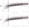 |
Fig. A.1 Hipparcos absolute magnitudes vs. distance distributions (up = MV, down = MI). The red curves indicate the absolute magnitude completeness limit as a function of the distance. The vertical line shows our distance limit to get the local stellar population. The horizontal full lines at MV = 0 and MV = 6 correspond to the domain that contains enough stars from the Hipparcos catalog to enable our debiasing procedure. |
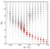 |
Fig. A.2 Hipparcos absolute color–magnitude diagram in MIC vs. (V − I)J. The black squares correspond to the full catalog (statistically biased). The red squares correspond to the subsample of stars closer than 50 pc; this subsample is statistically unbiased only for absolute magnitude MV< 4.0 (corresponding to MI< 3.1, above the horizontal line in the diagram). The size scales are different between the red and black squares for readability. |
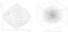 |
Fig. A.3 Two-dimensional and 3D distributions of the Hipparcos objects within 50 pc. The excess toward (α = 67°δ = 16°) corresponds to the Hyades open cluster. |
The upper panels of Fig. A.4 show the absolute magnitude and color distributions of all the Hipparcos stars within 50 pc (full lines) and of the stars that are closer than min(dc(MV),50 pc), where dc(MV) is the completion distance defined in Eq. (A.1) (dashed red lines).
We represent the Hipparcos catalog as a multi-dimensional distribution function defined by 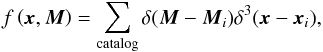 (A.2)where xi is the position of star i and Mi represents its absolute magnitude and color “vector” (i.e., its type). As explained above, to extract the unbiased local density for a given stellar type characterized by the vector M (here (MI,MV)), we only account for the objects that are both within the completion volume (d<dc(MV)) and closer than 50 pc, i.e.,
 ![\appendix \setcounter{section}{1} \begin{eqnarray} n(\vec{M})&=& \frac{3}{4\pi .\min[{d_{c}(M_V)}, 50~\mathrm{pc}]^3} \nonumber\\&& \times\int_{d< \min[{d_{c}(M_V)}, 50~\mathrm{pc}]} f( \vec{x},\vec{M}) k(d) {\rm d}^3 x, \end{eqnarray}](/articles/aa/full_html/2017/08/aa30488-17/aa30488-17-eq339.png) (A.3)where k(d) is a correction factor that takes into account the variation of the density within the completion volume (this correction varies from 1 to 1.09).
(A.3)where k(d) is a correction factor that takes into account the variation of the density within the completion volume (this correction varies from 1 to 1.09).
Appendix A.1: Extrapolating the local HIPPARCOS CMD
The number of usable Hipparcos objects (closer than min(dc(MV),50 pc)) is statistically limited in the faint (MV> 6) and bright (MV< 0) ends, as can be seen in Fig. A.4 (upper left, dashed line). Moreover, there is no star with MV> 9 within its corresponding completion distance dc(9) ≃ 5 pc (i.e., above the red curve of Fig. A.1), because the volume is too small; there is also no local star (within 50 pc) brighter than MV = − 3.
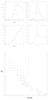 |
Fig. A.4 Top: raw distributions of MV and (V − I) of all Hipparcos stars within 50 pc (6911 objects). The dashed lines show the numbers of stars within the completion volume corresponding to their magnitude (see text). Middle: local debiased volumic density of stars (per magnitude unit, in pc-3) estimated from the ratio of stars within the completion volume and extrapolated beyond MV = 6. Bottom: debiased MV vs. V − I stellar density of stars closer than 50 pc. |
Therefore, when building a debiased density color–magnitude diagram, we need to examine specifically the contribution of the stars with absolute MV magnitudes out of [ 0,6 ] range to avoid statistical limitations or biases:
-
First, we can neglect the contribution of the brightest stars;indeed, the Hipparcos catalog contains only 35 stars brighter thanMV< 0 within 50 pc (complete sample). This corresponds to a maximum contribution of
![\appendix \setcounter{section}{1} \begin{equation} 35\times\left[\frac{10~\mathrm{kpc}}{50~\mathrm{pc}}\right]^3\times\frac{\Omega (1\degree \times 1\degree)}{4\pi}\sim 6800\, {\rm stars/sq\, deg} \end{equation}](/articles/aa/full_html/2017/08/aa30488-17/aa30488-17-eq351.png) (A.4)of MV< 0 stars within 10 kpc distance (typically less than 2 − 3% toward the directions studied in this paper). This contribution will be neglected in the following discussions5.
(A.4)of MV< 0 stars within 10 kpc distance (typically less than 2 − 3% toward the directions studied in this paper). This contribution will be neglected in the following discussions5. -
Stars fainter than MV = 6 have a minor, but not negligible contribution to a deep Galatic exposure. Instead of debiasing the statistically limited subsample of the Hipparcos catalog, we choose to linearly extrapolate the local stellar density of these faint stars as (see Fig. A.4 middle, left):
 (A.5)Since we deduce from Fig. A.2 (lower right branch) that
  (A.6)or equivalently
  (A.7)the type of these faint stars is also completely extrapolated.
Figure A.4 (bottom) shows the local CMD obtained following our complete procedure using the Hipparcos stars with 0 <MV< 6 within dc(MV) and our extrapolated distribution for 6 <MV< 8.
Appendix A.2: Comparison with the stellar density expected from the mass function: A coherence check
We can crosscheck the stellar number density found from the Hipparcos catalog and the density expected from the mass function as follows: stars with 0 <MV< 6 belong to the mass domain defined by 0.85 M⊙<m< 2.8 M⊙ (Delfosse et al. 2000). The local number density of objects within this mass range is given by  (A.8)where
  is the stellar mass function in the solar neighborhood. We use the mass function
  of Chabrier (2003), revised in Chabrier (2004),
 ![\appendix \setcounter{section}{1} \begin{eqnarray} \xi(\log m/\Msol)&=& 0.093\times \exp\left[ \frac{-(\log m/0.2~\Msol)^2}{2\times (0.55)^2}\right],\,m\le \Msol \nonumber \\ &=&0.041 (m/\Msol)^{-1.35},\,m> \Msol \label{chabrierfunction} \end{eqnarray}](/articles/aa/full_html/2017/08/aa30488-17/aa30488-17-eq362.png) (A.9)(see Fig. 8). We find that the mean density of disk stars with 0 <MV< 6 in a sphere of 50 pc centered on the sun (located at 26 pc from the disk plane, Majaess et al. 2009) is 0.012 pc-3. This is compatible with the estimates from the integral of the MV debiased distribution of the volumic density of stars plotted in Fig. A.4, nHipparcos = 0.0076 pc-3, when taking into account the fact that ~2:3 of the stars are in binary systems (Chabrier 2004) not deblended in the Hipparcos observations.
(A.9)(see Fig. 8). We find that the mean density of disk stars with 0 <MV< 6 in a sphere of 50 pc centered on the sun (located at 26 pc from the disk plane, Majaess et al. 2009) is 0.012 pc-3. This is compatible with the estimates from the integral of the MV debiased distribution of the volumic density of stars plotted in Fig. A.4, nHipparcos = 0.0076 pc-3, when taking into account the fact that ~2:3 of the stars are in binary systems (Chabrier 2004) not deblended in the Hipparcos observations.
Appendix B: Parameters of the Besançon Galactic model
The Sun is located at R⊙ = 8.0 kpc and z⊙ = 15 pc, which is different than in our simple model. The thin disk structures are parametrized in cylindrical galactocentric coordinates (r,z), and for various ranges of age, as follows: ![\appendix \setcounter{section}{2} \begin{eqnarray} \rho_{D}(r,z)_{\rm age} &\propto& \left[ \exp\left(-\frac{a^2}{R_d^2} \right) -\exp\left(-\frac{a^2}{R_h^2} \right) \right]~\mathrm{if~age<0.15~Gyr}, \nonumber \\ &\propto& \left[ \exp\left(- \sqrt{0.25 + \frac{a^2}{R_d^2}}\right) -\exp\left(-\sqrt{0.25 +\frac{a^2}{R_h^2}}\right) \right], \nonumber \\ && \mathrm{if~age>0.15~Gyr,} \end{eqnarray}](/articles/aa/full_html/2017/08/aa30488-17/aa30488-17-eq369.png) (B.1)where
(B.1)where
-
Rd = 5.0 kpc and Rh = 3.0 kpc if age < 0.15 Gyr;
-
Rd = 2.17 kpc and Rh = 1.33 kpc if age > 0.15 Gyr;
-
a2 = r2 + (z/ϵage)2;
-
ϵage and the local mass densities corresponding to ρD(r⊙,z⊙)age values are given in Table B.1 for the different ranges of stellar age, together with the IMFs.
The thick disk contribution is expressed by ![\appendix \setcounter{section}{2} \begin{eqnarray} \rho_{D}^{\rm thick}(r,z) &=& \rho_{D}^{\rm thick}(r_{\odot},z_{\odot}) \nonumber \\ && \times \left(1-\frac{z^2}{x_l (2h_z+x_l)}\right) \exp\left[-\frac{r-R_{\odot}}{R_{\rm thick}} \right]~\mathrm{if}~|z|<x_l, \nonumber\\ & & \times \frac{\exp(x_l/h_z)}{1+x_l/2h_z}\exp\left[-\frac{|z|}{h_z}\right] \exp \left[ -\frac{r-R_{\odot}}{R_{\rm thick}} \right]~ \mathrm{if}~|z|>x_l, \end{eqnarray}](/articles/aa/full_html/2017/08/aa30488-17/aa30488-17-eq379.png) (B.2)
(B.2)
where xl = 400 pc, hz = 800 pc and Rthick = 2.5 Kpc. Table B.1 also gives the total local densitiy  for the thick disk together with the IMF.
The two components of the bar are described in a Cartesian frame positioned at the Galactic center with the major axis X tilted by Φ = 12.8 degree with respect to the Galactic center-Sun direction. The mass density for each component of the bar is given by (Robin et al. 2012)  where
where ![\appendix \setcounter{section}{2} \begin{equation} R_s^{C_p}= \left[\left| \frac{X}{a}\right|^{C_n} + \left| \frac{Y}{b}\right|^{C_n} \right]^{\frac{C_p}{C_n}} + \left| \frac{Z}{c}\right|^{C_p}, \\ \end{equation}](/articles/aa/full_html/2017/08/aa30488-17/aa30488-17-eq386.png) (B.5)and fc is a cutoff function
(B.5)and fc is a cutoff function ![\appendix \setcounter{section}{2} \begin{eqnarray} f_c(X,Y)&=&1.~~~\mathrm{if}~X^2+Y^2<R_c^2, \\ &=&\exp\left[ -\frac{(\!\sqrt{X^2+Y^2}-R_C)^2}{0.25\,\rm{kpc}^2}\right]~\mathrm{if}~X^2+Y^2>R_c^2. \nonumber \end{eqnarray}](/articles/aa/full_html/2017/08/aa30488-17/aa30488-17-eq388.png) (B.6)The parameters for bar1 are ρ0 = 9.21 M⊙ pc-3 (6), with scale length factors a = 1.46 kpc, b = 0.49 kpc, c = 0.39 kpc, Rc = 3.43 kpc, and Cp = 3.007, Cn = 3.329. The total mass of this bar is 35.45 × 10⁹M⊙.
(B.6)The parameters for bar1 are ρ0 = 9.21 M⊙ pc-3 (6), with scale length factors a = 1.46 kpc, b = 0.49 kpc, c = 0.39 kpc, Rc = 3.43 kpc, and Cp = 3.007, Cn = 3.329. The total mass of this bar is 35.45 × 10⁹M⊙.
The parameters for bar2 are ρ0 = 0.026 M⊙ pc-3, with scale length factors a = 4.44 kpc, b = 1.31 kpc, c = 0.80 kpc, Rc = 6.83 kpc, and Cp = 2.786, Cn = 3.917. The total mass of this bar is 2.27 × 10⁹M⊙. The IMF for these two bars is dn/ dm ∝ (m/M⊙)-2.35.
Age, local mass density ρ(r⊙,z⊙), disk axis ratio ϵ, and IMF of the different stellar components of the disks in the Besançon model. WD represents the white dwarfs.
As far as kinematics is concerned, we use the ellipsoids of velocity dispersions provided for each structure and age in Table 4 of (Robin et al. 2003).
All Tables
Best fit results on the observables toward the 4 regions monitored in the EROS spiral arms program, compared with previous simulations (model 1) and observations published in Rahal et al. (2009b).
Age, local mass density ρ(r⊙,z⊙), disk axis ratio ϵ, and IMF of the different stellar components of the disks in the Besançon model. WD represents the white dwarfs.
All Figures
|
Fig. 1 Four directions toward the Galactic spiral arms monitored by EROS. |
| In the text | |
|
Fig. 2 Time sampling toward the 4 monitored targets in the Galactic spiral arms: average number of measurements per star and per week. |
| In the text | |
|
Fig. 3 Relative color–magnitude diagrams n(I,V − I) of the EROS catalogs toward the 4 directions toward the Galactic spiral arms. The gray scale gives the number density of stars per square degree, unit of magnitude, and unit of color index. |
| In the text | |
|
Fig. 4 Star detection probability in EROS vs. the relative magnitude BEROS = I + 0.6(V − I). |
| In the text | |
|
Fig. 5 Photometric point-to-point precision along the EROS light-curves vs. REROS = I (upper) and BEROS (lower). Vertical bars in I show the dispersion of this precision in the EROS catalog. The histograms show the magnitude distribution of the full EROS spiral arm catalog (all directions). |
| In the text | |
|
Fig. 6 Microlensing detection efficiency of the EROS survey toward the Galactic spiral arms, as a function of the event characteristic duration tE. |
| In the text | |
|
Fig. 7 The V − I observed (gray histograms) and the simulated distributions (simple model in black, Besançon model in red) for the bright stars (with I< 18.4), using the Marshall table without systematic/statistical uncertainties (to be compared with Fig. 10, bottom). |
| In the text | |
|
Fig. 8 Different mass functions considered in this paper: Standard Chabrier (black) corresponds to the local regular Chabrier IMF (Eq. (A.9) with m0 = 0.2 M⊙); the modified Chabrier (m0 = 0.51 M⊙, in green) gives the best fit for the lens IMF from our simple model. |
| In the text | |
|
Fig. 9 Mass-density along the line of sight of γSct from the various Galactic structures (disks and bar), as a function of the distance from the Sun for our nominal simple model (thin black lines) and the Besançon model (thick blue lines). The total densities are shown with dashed lines. |
| In the text | |
|
Fig. 10 Simulated CMDs toward the 4 monitored directions (top) with the magnitude (middle) and color (bottom) projections for the stars brighter than I = 18.4, expressed in million of stars per square degree per magnitude. Results from our simple model are plotted with black lines and results from the Besançon model with red lines; the distributions of the EROS observed populations of bright stars (I< 18.4) are superimposed on the projections as light gray histograms. |
| In the text | |
|
Fig. 11 Simulated optical depths toward the 4 monitored directions, as a function of the source distance, for our nominal simple model (thin lines) and the Besançon model (thick lines). |
| In the text | |
|
Fig. 12 Expected normalized distributions of the distances for the lensed sources – when taking into account the EROS microlensing detection efficiencies – (thin lines) and of the lenses (thick lines) from the simulation of our simple model (upper) and the Besançon model (lower). The sparsely-populated distributions around 4 kpc (for β Sct and γ Sct) correspond to the contribution of the bar objects. The dashed curves show, as a function of the distance, the average extinctions of the stars in the simulated EROS-like catalog (in V magnitude, on the right scale). It is strongly biased in favor of small extinctions mainly due to the magnitude selection I< 18.4. |
| In the text | |
|
Fig. 13 Einstein duration tE distribution of the microlensing events expected by assuming 4 different IMFs: the standard Chabrier (black), the Besançon model (red), the modified Chabrier (with m0 = 0.57, green), and the Kroupa IMF (blue). |
| In the text | |
|
Fig. A.1 Hipparcos absolute magnitudes vs. distance distributions (up = MV, down = MI). The red curves indicate the absolute magnitude completeness limit as a function of the distance. The vertical line shows our distance limit to get the local stellar population. The horizontal full lines at MV = 0 and MV = 6 correspond to the domain that contains enough stars from the Hipparcos catalog to enable our debiasing procedure. |
| In the text | |
|
Fig. A.2 Hipparcos absolute color–magnitude diagram in MIC vs. (V − I)J. The black squares correspond to the full catalog (statistically biased). The red squares correspond to the subsample of stars closer than 50 pc; this subsample is statistically unbiased only for absolute magnitude MV< 4.0 (corresponding to MI< 3.1, above the horizontal line in the diagram). The size scales are different between the red and black squares for readability. |
| In the text | |
|
Fig. A.3 Two-dimensional and 3D distributions of the Hipparcos objects within 50 pc. The excess toward (α = 67°δ = 16°) corresponds to the Hyades open cluster. |
| In the text | |
|
Fig. A.4 Top: raw distributions of MV and (V − I) of all Hipparcos stars within 50 pc (6911 objects). The dashed lines show the numbers of stars within the completion volume corresponding to their magnitude (see text). Middle: local debiased volumic density of stars (per magnitude unit, in pc-3) estimated from the ratio of stars within the completion volume and extrapolated beyond MV = 6. Bottom: debiased MV vs. V − I stellar density of stars closer than 50 pc. |
| In the text | |
Current usage metrics show cumulative count of Article Views (full-text article views including HTML views, PDF and ePub downloads, according to the available data) and Abstracts Views on Vision4Press platform.
Data correspond to usage on the plateform after 2015. The current usage metrics is available 48-96 hours after online publication and is updated daily on week days.
Initial download of the metrics may take a while.