| Issue |
A&A
Volume 603, July 2017
|
|
|---|---|---|
| Article Number | L1 | |
| Number of page(s) | 5 | |
| Section | Letters | |
| DOI | https://doi.org/10.1051/0004-6361/201731121 | |
| Published online | 06 July 2017 | |
NH3 (10–00) in the pre-stellar core L1544⋆
1 Centre for Astrochemical Studies, Max-Planck-Institute for Extraterrestrial Physics, Giessenbachstrasse 1, 85748 Garching, Germany
e-mail: caselli@mpe.mpg.de
2 INAF–Osservatorio Astrofisico di Arcetri, Largo E. Fermi 5, 50125 Firenze, Italy
3 Harvard-Smithsonian Center for Astrophysics, 60 Garden Street, Cambridge, MA 02138, USA
4 Observatorio Astronómico Nacional (IGN), Calle Alfonso XII, 3 Madrid, Spain
5 LERMA and UMR 8112 du CNRS, Observatoire de Paris, 61 Av. de l’Observatoire, 75014 Paris, France
6 Centre for Star and Planet Formation, Niels Bohr Institute and Natural History Museum of Denmark, University of Copenhagen, Øster Voldgade 5–7, 1350 Copenhagen, Denmark
7 SRON Netherlands Institute for Space Research, Landleven 12, 9747 AD Groningen, The Netherlands
8 Kapteyn Astronomical Institute, University of Groningen, The Netherlands
9 The Dublin Institute for Advanced Studies, 31 Fitzwilliam Place, Dublin 2, Ireland
10 INAF–Osservatorio Astronomico di Roma, 00040 Monte Porzio Catone, Italy
11 Center for Computational Science, University of Tsukuba, Tsukuba, 305-8577 Ibaraki, Japan
12 Université Grenoble Alpes, CNRS, IPAG, 38000 Grenoble, France
13 Leiden Observatory, Leiden University, PO Box 9513, 2300 RA Leiden, The Netherlands
Received: 7 May 2017
Accepted: 8 June 2017
Pre-stellar cores represent the initial conditions in the process of star and planet formation, therefore it is important to study their physical and chemical structure. Because of their volatility, nitrogen-bearing molecules are key to study the dense and cold gas present in pre-stellar cores. The NH3 rotational transition detected with Herschel-HIFI provides a unique combination of sensitivity and spectral resolution to further investigate physical and chemical processes in pre-stellar cores. Here we present the velocity-resolved Herschel-HIFI observations of the ortho-NH3(10 − 00) line at 572 GHz and study the abundance profile of ammonia across the pre-stellar core L1544 to test current theories of its physical and chemical structure. Recently calculated collisional coefficients have been included in our non-LTE radiative transfer code to reproduce Herschel observations. A gas-grain chemical model, including spin-state chemistry and applied to the (static) physical structure of L1544 is also used to infer the abundance profile of ortho-NH3. The hyperfine structure of ortho-NH3(10 − 00) is resolved for the first time in space. All the hyperfine components are strongly self-absorbed. The profile can be reproduced if the core is contracting in quasi-equilibrium, consistent with previous work, and if the NH3 abundance is slightly rising toward the core centre, as deduced from previous interferometric observations of para-NH3(1, 1). The chemical model overestimates the NH3 abundance at radii between ≃4000 and 15 000 AU by about two orders of magnitude and underestimates the abundance toward the core centre by more than one order of magnitude. Our observations show that chemical models applied to static clouds have problems in reproducing NH3 observations.
Key words: astrochemistry / line: profiles / radiative transfer / methods: observational / ISM: clouds / ISM: molecules
© ESO, 2017
1. Introduction
Since its discovery as the first polyatomic molecule in space (Cheung et al. 1968), ammonia has been widely used as a temperature and structural probe of dense cloud cores in low-mass (e.g. Benson & Myers 1989) and high-mass (e.g. Pillai et al. 2006) star-forming regions, and as a tracer of shocks along outflows driven by young stellar objects (e.g. Tafalla & Bachiller 1995). NH3 can form on the surface of dust grains through hydrogenation of atomic nitrogen and in the gas phase soon after the formation of N2. Unlike molecules such as CO, NH3 does not appear to be affected by freeze-out within dense and cold starless cores (Tafalla et al. 2002), despite its high binding energies (close to those of H2O). While the inversion transitions of ortho (o) and para (p) NH3 around 1.3 cm are easily accessible from the ground, the rotational transitions fall into the sub-millimeter and far-IR, and these can only be detected using space-borne receivers. The Einstein coefficients of the rotational transitions of NH3 are about 10 000 times larger than those of the inversion transitions (Ho & Townes 1983), implying significantly higher critical densities (≃107 cm-3 vs. ≃103 cm-3; Danby et al. 1988).
The first observation of the ground-state rotational transition of o-NH3(10 − 00) was carried out by Keene et al. (1983) toward OMC-1 using the Kuiper Airborne Observatory (KAO). About twenty years later, the Odin satellite detected o-NH3(10 − 00) toward the Orion Bar (Larsson et al. 2003), high-mass star-forming regions (Hjalmarson et al. 2005; Persson et al. 2007, 2009) and, for the first time, toward a dark cloud (ρ Oph A; Liseau et al. 2003). Multiple rotational transitions have also been detected using the Heterodyne Instrument for the Far Infrared (HIFI; de Graauw et al. 2010) instrument on board the Herschel Space Observatory in the direction of high-mass star forming regions (Persson et al. 2010; Gerin et al. 2016) and with the Infrared Space Observatory (ISO; Ceccarelli et al. 2002). The o-NH3(10 − 00) has also been detected with Herschel by Codella et al. (2010) toward the shock region L1157-B1, by Salinas et al. (2016) toward the protoplanetary disk TW Hydrae, and by Lis et al. (2016) in the direction of the starless core L1689N, next to the young protostar IRAS16293-2422. None of the above spectra show resolved hyperfine structure of o-NH3, including the one toward L1689N, where only one group of hyperfine components is detected. The 32 − 22 rotational transition of NH3 at 1.8 THz has also been observed with the Stratospheric Observatory For Infrared Astronomy (SOFIA) by Wyrowski et al. (2012, 2016) to measure the infall rate in high-mass star-forming clumps.
We report the first detection of the hyperfine structure of o-NH3(10 − 00) toward the isolated pre-stellar core L1544 in the Taurus molecular cloud complex, as part of the Water In Star-forming regions with Herschel (WISH) key project (van Dishoeck et al. 2011). The turbulence in L1544 is subsonic and the narrow spectral line widths, together with the high spectral resolution of HIFI, allow us to distinguish the quadrupole hyperfine structure that is due to the interaction between the molecular electric field gradient and the electric quadrupole moment of the nitrogen nucleus. These observations also confirm the dynamical structure that has been deduced by previous theoretical studies (Keto & Caselli 2008, 2010; Keto et al. 2015) constrained by ground-based (Caselli et al. 1999, 2002) and Herschel (Caselli et al. 2010, 2012) observations. In the following, we refer to the core envelope as the region beyond ≃4000 AU, where the number density drops below 105 cm-3 (Keto & Caselli 2010). Observations are described in Sect. 2, the o-NH3(10 − 00) spectrum is shown in Sect. 3 and the analysis is presented in Sect. 4. Discussion and conclusions can be found in Sect. 5.
2. Observations
The o-NH3(10 − 00) line (central frequency 572.49815977 GHz ±0.2 kHz; Cazzoli et al. 2009) has been observed with Herschel toward the pre-stellar core L1544 (coordinates RA(J2000) = 05h04m17 21, Dec(J2000) = 25°10′42.̋8) for 10.3 h on April 2, 2011, together with the o-H2O(110 − 101) (Caselli et al. 2012). The data presented here are archived at the Herschel science archive1 with the identification number (OBSID) 1342217688. The technical details of the observations, which include the simultaneous use of the wide-band (WBS) and the high-resolution (HRS) spectrometers of HIFI in both H and V polarisation, have been described in Caselli et al. (2012). We briefly summarise the details related to the HRS data for o-NH3, which are used here: the half-power beam width (HPBW) of the telescope at 572 GHz is 40′′ and the spectral (nominal) resolution is 64 m s-1 at 572.5 GHz. The individual spectra were reduced using the Herschel interactive processing environment (HIPE; Ott 2010), version 14.1, and subsequent analysis of the data was performed with the Continuum and Line-Analysis Single dish Software (CLASS) within the GILDAS package2. The latest in-flight-measured beam efficiencies were used to convert the intensity scale from antenna temperature into main-beam temperature (Tmb) 3. The H and V polarisation spectra are identical and they have been summed together to increase the sensitivity.
3. Results
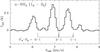 |
Fig. 1 Herschel HIFI spectrum of o-NH3(10 − 00) toward the pre-stellar core L1544. The three groups of hyperfine components (with the 0−1 group having one single component) are detected for the first time in space. They are all highly self-absorbed (see Sect. 3). The hyperfine structure is shown by black vertical lines (with LTE relative intensities) and labelled as in Cazzoli et al. (2009). The vertical dotted line marks the core velocity. The root-mean-square noise level is 4.7 mK. |
The continuum-subtracted o-NH3(10 − 00), centred at the frequency of the main hyperfine component (572.4983387 GHz), is shown in Fig. 1 together with the hyperfine structure from Table 3 of Cazzoli et al. (2009), adopting the Local Standard of Rest (LSR) velocity (VLSR) of L1544, 7.2 km s-1, as reported by Tafalla et al. (1998). This is the first observed interstellar o-NH3(10 − 00) spectrum clearly showing the main groups of hyperfine components. The mismatch between the VLSR and the centroid velocity of the main group of hyperfine components is due to heavy self-absorption (from the envelope) combined with Doppler-shifted emission (due to core contraction; Keto & Caselli 2010). In fact, NH3 is abundant across L1544 (Crapsi et al. 2007), and the outer portions of the contracting pre-stellar core, where the volume density is significantly lower than the critical density of o-NH3(10 − 00), are absorbing the redshifted part of the spectrum that is emitted toward the centre.
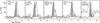 |
Fig. 2 Comparison between the isolated hyperfine component |

Self-absorption and Doppler-shifting due to the dynamics have already been detected in other molecular lines when observed toward the same line of sight. Figure 2 shows a comparison of the only isolated hyperfine component in the spectrum of o-NH3(10 − 00) ( →FN = 0 → 1; filled grey histogram) with other lines: C18O(1−0), o-H2D+(110 − 111), N2H+(1−0), HCO+(1−0), and o-H2O(110 − 101) (black histograms). The o-NH3 hyperfine component displays the characteristic blue-shifted infall profile (e.g. Evans 1999), with a self-absorption dip reaching the zero-level, thus indicating a large line optical depth (Myers et al. 1996). It is interesting to note that the NH3 line shows extra emission at low velocities (coming from the material approaching the core centre from the back) when compared to the low-density tracer C18O(1−0), which does not probe the central regions because of the large CO freeze-out (Caselli et al. 1999). Extra blue emission of the o-NH3(10 − 00) hyperfine component is also seen when compared to the o-H2D+(110 − 111) and N2H+(1−0) lines, although to a lesser extent. The “blue excess” disappears in the case of HCO+(1−0), which is also heavily absorbed (Tafalla et al. 1998). The resemblance between o-NH3(10 − 00) and HCO+(1−0) is quite striking, in view of the fact that the distribution of HCO+ across the core is known to be quite different from that of NH3, with HCO+ tracing the outer layers of the core while being depleted toward the centre because of the freeze-out of its main parent species CO (Tafalla et al. 2002, 2006). The H2O line is the most blue-shifted and displays the broadest absorption, thus suggesting higher optical depths (see Keto et al. 2014). This is probably caused by the large abundance of H2O (compared to NH3) in the L1544 outer layers, which is responsible for the absorption in a velocity range spanned by the lower density tracers in Fig. 2.
4. Analysis
The non-local thermal equilibrium (non-LTE) radiative transfer code MOLLIE (Keto 1990; Keto et al. 2004; Keto & Rybicki 2010) was used to interpret the o-NH3(10 − 00) spectrum in Fig. 1. We took into account the hyperfine structure, produced by the electric quadrupole coupling of the N nucleus with the electric field of the electrons, as well as the magnetic hyperfine structure that is due to the three protons (Cazzoli et al. 2009). The hyperfine collision rate coefficients were taken from the recent calculations of Bouhafs et al. (2017), which, for the first time, include the non-spherical structure of p-H2 (the main form of H2 in cold molecular gas, Flower et al. 2006; Brünken et al. 2014), so that they differ (by up to a factor ≃2) from those of Maret et al. (2009). The calculations were restricted to the lowest nine hyperfine levels of o-NH3, corresponding to the first two rotational levels (00 and 10), within a temperature range 5−30 K. Since only the ground-state o-NH3 transitions were considered, no scaling of the rotational rates was necessary: all hyperfine rates are equal to the pure rotational rates, and intra-multiplet rates are set to zero, as in the standard statistical approach.
Unlike for H2O and CO (Keto & Caselli 2008; Caselli et al. 2012; Keto et al. 2014), we did not develop any simplified chemistry for NH3 to be coupled with the hydro-dynamical evolution. Two different approaches were followed to simulate the observed spectrum: (1) the radial profile of o-NH3 follows that of p-NH3 deduced by Crapsi et al. (2007) using VLA observations of p-NH3(1,1), assuming an ortho-to-para NH3 abundance ratio of 1 and 0.74, and extrapolating to larger radii (see Eq. (1)); (2) the radial profile of o-NH3 was calculated using the chemical model predictions of Sipilä et al. (2015a,b) and Sipilä et al. (2016) applied to the L1544 physical structure deduced by Keto & Caselli (2010) and Keto et al. (2015), who demonstrated that other observed line profiles can be reproduced by the quasi-equilibrium contraction of an unstable Bonnor-Ebert sphere. The two abundance profiles are presented in Fig. 3 together with the profile of H2O deduced by Caselli et al. (2012) and refined by Keto et al. (2014).
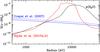 |
Fig. 3 Radial profile of the fractional abundance of o-NH3 with respect to H2, X(o-NH3), in L1544. The blue profile has been deduced from observations carried out by Crapsi et al. (2007) assuming an ortho-to-para NH3 abundance ratio of 1 (dashed curve) and 0.7 (solid curve); the red profile is the result of a chemical model calculation by Sipilä et al. (2015a,b). The black profile refers to the total (ortho+para) abundance of H2O from Keto et al. (2014). |
Crapsi et al. (2007) followed the same analysis as Tafalla et al. (2002). They parametrised the abundance profile of total (ortho+para) NH3, XNH3(r), starting from X(p-NH3) and assuming an ortho-to-para ratio of unity, with the function: 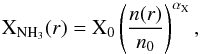 (1)and then finding the best-fit parameters: X0 = 8 × 10⁻⁹, n0 = 2.1 × 106 cm-3 (the average density within a radius of 14″) and αX = 0.16. The abundance profile of p-NH3 measured by Crapsi et al. (2007) is given by multiplying the right-hand side of Eq. (1) by 0.5; from this, we derived the abundance profile of o-NH3 assuming an ortho-to-para NH3 ratio of 1 (dashed blue curve in Fig. 3) and 0.7 (solid blue curve in Fig. 3). The latter value is expected in cold gas and would indicate a gas-phase formation for NH3 (Faure et al. 2013). As noted by Tafalla et al. (2002), Crapsi et al. (2007) found that the NH3 abundance slightly increases toward the core centre. We note that the interferometric observations of Crapsi et al. (2007) have an angular resolution of about 4′′ (~300 AU in radius), so they place stringent constraints on the abundance profile of NH35. A comparison of the blue curves with the (ortho+para) H2O abundance profile deduced by Keto et al. (2014) (black curve in Fig. 3) shows that the total NH3 is about 30 times more abundant than H2O within the central 1000 AU, while it is two orders of magnitude less abundant than H2O from about 8000 AU to 20 000 AU.
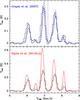 |
Fig. 4 MOLLIE radiative transfer results using the o-NH3 fractional abundance profiles from Fig. 3, overlapped with the observed spectrum: (top) blue solid and dashed curves refer to the Crapsi et al. (2007) profiles, assuming an ortho-to-para NH3 ratio of 0.7 and 1.0, respectively. (Bottom) The red thick curve refers to the Sipilä et al. (2015a,b) profile; the red thin curve is the same as the thick red curve, but divided by 2. |
The o-NH3 profile has a very different shape when the chemical model of Sipilä et al. (2015a,b), which includes spin-state chemistry, is considered (red curve in Fig. 3). The chemical abundance gradients in L1544 were simulated using the same procedure as described in Sipilä et al. (2016): the physical model for L1544 (Keto & Caselli 2010; Keto et al. 2014) was separated into concentric shells and the chemical evolution was calculated separately in each shell. The gas was initially atomic with the exception of H (all in H2) and D (in HD). The o-NH3 abundance profile (Fig. 3) was extracted from the model at the time when the CO column density was comparable to the observed value (1.3 × 1018 cm-2; see Caselli et al. 1999), taking into account telescope beam convolution. Other details of the chemical model are extensively discussed in Sipilä et al. (2015a,b). The predicted o-NH3 profile (red curve in Fig. 3) presents a broad peak between 5000 AU and 15 000 AU, it drops at larger radii because of photodissociation and at lower radii because of freeze-out.
The o-NH3(10 − 00) spectra simulated with MOLLIE are shown in Fig. 4 for the three o-NH3 abundance profiles in Fig. 3, together with the observed spectrum. This figure shows that the empirical abundance profile of Crapsi et al. (2007) reproduces the observed spectrum better than the abundance profile predicted by Sipilä et al. (2015a,b), although the simulated spectrum underestimates the brightness temperature at the lowest velocities of all groups of hyperfine components, as also found in the case of o-H2O (Caselli et al. 2012), which suggests that the contraction velocity within the core centre is slightly higher than the velocity used in our model. The red spectrum (based on the chemical model of Sipilä et al. 2015a,b) is significantly brighter than the detected line and the ratios between the low- and high-velocity peaks of the various hyperfine components are not well reproduced (as better shown by the red thin curve in Fig. 4, which is the red thick profile scaled down by a factor of two). It is interesting to note that the red curve is shifted to lower velocities than the blue curves. This is due to the large abundance of NH3 predicted at radii in the range of 4000−12 000 au (Fig. 3, red curve), which produces a bright optically thick line and causes absorption around the core LSR velocity, as the contraction velocity is lower in the core envelope, which produces the absorption (Keto & Caselli 2010).
5. Discussion and conclusions
Herschel observations of the o-NH3(10 − 00) line toward the dust peak of the L1544 pre-stellar core have been presented. The spectrum shows for the first time the three well-separated groups of hyperfine components. The three components are strongly self-absorbed and display the characteristic infall profile, with a blue peak significantly brighter than the red peak and a dip reaching the zero level, although for the →FN = 2 → 1 components, the red peak is blended with the blue peak of the 1−1 component. The observed spectrum can be well reproduced adopting the empirical NH3 abundance profile deduced by the interferometric observations of Crapsi et al. (2007) as well as the physical structure that was used to reproduce previous spectra: the Bonnor-Ebert sphere in quasi-static contraction, which is characterised by a central density of 107 cm-3 and a subsonic contraction velocity field peaking at a radius of 1000 AU (Keto & Caselli 2010; Caselli et al. 2012; Keto et al. 2015).
A poorer match with observations is seen when the o-NH3 profile predicted by the comprehensive chemical model of Sipilä et al. (2015a,b), applied to the (static) physical structure of L1544, is used as input in MOLLIE. This suggests that “pseudo-time dependent” chemical models (i.e. time-dependent chemical models applied to static clouds) have problems in reproducing the observed chemical structure of pre-stellar cores. The model predicts too much NH3 in the outer parts of the cloud6 and too little toward the centre, when compared with the abundance deduced by the interferometric observations of Crapsi et al. (2007). The predicted large NH3 abundance at radii around 10 000 AU is mainly caused by surface formation followed by reactive desorption (with 1% efficiency, which may be overestimated). Figure 2 shows that the o-H2O spectrum is more absorbed around the LSR velocity than that of o-NH3, suggesting that H2O is indeed more extended than NH3 in the outer low-density part of the envelope, while the red curve in Fig. 3 predicts NH3 abundances around 10 000 AU comparable to those of H2O (see Fig. 3). Toward the core centre, the predicted low NH3 abundance indicates that selective desorption mechanisms for NH3 (e.g. lower binding energies for NH3 adsorbed on CO and/or N2 ice layers, formed on top of the water ice, combined with ice heating or disruptive action by cosmic rays; Ivlev et al. 2015), not included in the model, may be at work. Another possibility could be that the production of gas phase NH3 is underestimated; the N2 abundance profile drops more slowly than the CO abundance profile in the other pre-stellar core L183 (Pagani et al. 2012), meaning that N2 desorption is more efficient than currently advocated and/or that production of N2 is ongoing in the gas phase, thus maintaining efficient production of NH3 through the usual routes in the gas phase. However, the assumption of a static cloud could also be the cause of the discrepancy with the empirical profile, and this will be discussed in a future paper (Sipilä et al., in prep.). It is clear that more work needs to be done to gain understanding of the gas-grain chemical processes regulating NH3 and N-bearing molecules in cold and quiescent objects such as L1544, the precursors of future stellar systems.
Taking into account the calibration errors of the Crapsi et al. (2007) observations, we cannot distinguish between these two values. However, the two slightly different abundance profiles show how possible small variations in the abundance can affect the simulated spectrum.
Between 4000 and 15 000 AU. Above 20 000 AU, the NH3 abundance from Crapsi et al. (2007) is larger than that predicted by Sipilä et al. (2015a,b); however, this does not affect the model profile based on Eq. (1) in Fig. 4, as at radii >20 000 AU, the volume density is lower than 3000 cm-3, and the absorbing column is negligible.
Acknowledgments
P.C. acknowledges the financial support from the European Research Council (ERC; project PALs 320620). M.T. acknowledges partial support from MINECO project AYA2016-79006-P. C.M.W. acknowledges support from Science Foundation Ireland Grant 13/ERC/I2907. A.F. acknowledges support from the Agence Nationale de la Recherche (ANR-HYDRIDES), contract ANR-12-BS05-0011-01. HIFI has been designed and built by a consortium of institutes and university departments from across Europe, Canada and the United States under the leadership of SRON Netherlands Institute for Space Research, Groningen, The Netherlands and with major contributions from Germany, France and the US. Consortium members are: Canada: CSA, U. Waterloo; France: CESR, LAB, LERMA, IRAM; Germany: KOSMA, MPIfR, MPS; Ireland: NUI Maynooth; Italy: ASI, IFSI-INAF, Osservatorio Astrofisico di Arcetri-INAF; The Netherlands: SRON, TUD; Poland: CAMK, CBK; Spain: Observatorio Astronómico Nacional (IGN), Centro de Astrobiología (CSIC-INTA). Sweden: Chalmers University of Technology – MC2, RSS & GARD; Onsala Space Observatory; Swedish National Space Board, Stockholm University – Stockholm Observatory; Switzerland: ETH Zurich, FHNW; USA: Caltech, JPL, NHSC.
References
- Benson, P. J., & Myers, P. C. 1989, ApJS, 71, 89 [NASA ADS] [CrossRef] [Google Scholar]
- Bouhafs, N., Rist, C., Daniel, F. et al. 2017, MNRAS, in press DOI: https://doi.org/10.1093/mnras/stx1331 [Google Scholar]
- Brünken, S., Sipilä, O., Chambers, E. T., et al. 2014, Nature, 516, 219 [NASA ADS] [CrossRef] [PubMed] [Google Scholar]
- Caselli, P., Walmsley, C. M., Tafalla, M., Dore, L., & Myers, P. C. 1999, ApJ, 523, L165 [NASA ADS] [CrossRef] [Google Scholar]
- Caselli, P., Walmsley, C. M., Zucconi, A., et al. 2002, ApJ, 565, 331 [NASA ADS] [CrossRef] [Google Scholar]
- Caselli, P., Keto, E., Pagani, L., et al. 2010, A&A, 521, L29 [NASA ADS] [CrossRef] [EDP Sciences] [Google Scholar]
- Caselli, P., Keto, E., Bergin, E. A., et al. 2012, ApJ, 759, L37 [Google Scholar]
- Cazzoli, G., Dore, L., & Puzzarini, C. 2009, A&A, 507, 1707 [NASA ADS] [CrossRef] [EDP Sciences] [Google Scholar]
- Ceccarelli, C., Baluteau, J.-P., Walmsley, M., et al. 2002, A&A, 383, 603 [NASA ADS] [CrossRef] [EDP Sciences] [Google Scholar]
- Cheung, A. C., Rank, D. M., Townes, C. H., Thornton, D. D., & Welch, W. J. 1968, Phys. Rev. Lett., 21, 1701 [Google Scholar]
- Codella, C., Lefloch, B., Ceccarelli, C., et al. 2010, A&A, 518, L112 [NASA ADS] [CrossRef] [EDP Sciences] [Google Scholar]
- Crapsi, A., Caselli, P., Walmsley, M. C., & Tafalla, M. 2007, A&A, 470, 221 [NASA ADS] [CrossRef] [EDP Sciences] [Google Scholar]
- Danby, G., Flower, D. R., Valiron, P., Schilke, P., & Walmsley, C. M. 1988, MNRAS, 235, 229 [NASA ADS] [CrossRef] [Google Scholar]
- de Graauw, T., Helmich, F. P., Phillips, T. G., et al. 2010, A&A, 518, L6 [NASA ADS] [CrossRef] [EDP Sciences] [Google Scholar]
- Evans, II, N. J. 1999, ARA&A, 37, 311 [NASA ADS] [CrossRef] [Google Scholar]
- Faure, A., Hily-Blant, P., Le Gal, R., Rist, C., & Pineau des Forêts, G. 2013, ApJ, 770, L2 [NASA ADS] [CrossRef] [Google Scholar]
- Flower, D. R., Pineau Des Forêts, G., & Walmsley, C. M. 2006, A&A, 449, 621 [NASA ADS] [CrossRef] [EDP Sciences] [Google Scholar]
- Gerin, M., Neufeld, D. A., & Goicoechea, J. R. 2016, ARA&A, 54, 181 [NASA ADS] [CrossRef] [Google Scholar]
- Hjalmarson, Å., Bergman, P., Biver, N., et al. 2005, Adv. Space Res., 36, 1031 [NASA ADS] [CrossRef] [Google Scholar]
- Ho, P. T. P., & Townes, C. H. 1983, ARA&A, 21, 239 [NASA ADS] [CrossRef] [Google Scholar]
- Ivlev, A. V., Röcker, T. B., Vasyunin, A., & Caselli, P. 2015, ApJ, 805, 59 [NASA ADS] [CrossRef] [Google Scholar]
- Keene, J., Blake, G. A., & Phillips, T. G. 1983, ApJ, 271, L27 [NASA ADS] [CrossRef] [Google Scholar]
- Keto, E. R. 1990, ApJ, 355, 190 [NASA ADS] [CrossRef] [Google Scholar]
- Keto, E., & Caselli, P. 2008, ApJ, 683, 238 [NASA ADS] [CrossRef] [Google Scholar]
- Keto, E., & Caselli, P. 2010, MNRAS, 402, 1625 [NASA ADS] [CrossRef] [Google Scholar]
- Keto, E., & Rybicki, G. 2010, ApJ, 716, 1315 [NASA ADS] [CrossRef] [Google Scholar]
- Keto, E., Rybicki, G. B., Bergin, E. A., & Plume, R. 2004, ApJ, 613, 355 [NASA ADS] [CrossRef] [Google Scholar]
- Keto, E., Rawlings, J., & Caselli, P. 2014, MNRAS, 440, 2616 [NASA ADS] [CrossRef] [Google Scholar]
- Keto, E., Caselli, P., & Rawlings, J. 2015, MNRAS, 446, 3731 [NASA ADS] [CrossRef] [Google Scholar]
- Larsson, B., Liseau, R., Bergman, P., et al. 2003, A&A, 402, L69 [NASA ADS] [CrossRef] [EDP Sciences] [Google Scholar]
- Lis, D. C., Wootten, H. A., Gerin, M., et al. 2016, ApJ, 827, 133 [NASA ADS] [CrossRef] [Google Scholar]
- Liseau, R., Larsson, B., Brandeker, A., et al. 2003, A&A, 402, L73 [NASA ADS] [CrossRef] [EDP Sciences] [Google Scholar]
- Maret, S., Faure, A., Scifoni, E., & Wiesenfeld, L. 2009, MNRAS, 399, 425 [NASA ADS] [CrossRef] [Google Scholar]
- Myers, P. C., Mardones, D., Tafalla, M., Williams, J. P., & Wilner, D. J. 1996, ApJ, 465, L133 [NASA ADS] [CrossRef] [Google Scholar]
- Ott, S. 2010, in Astronomical Data Analysis Software and Systems XIX, eds. Y. Mizumoto, K.-I. Morita, & M. Ohishi, ASP Conf. Ser., 434, 139 [Google Scholar]
- Pagani, L., Bourgoin, A., & Lique, F. 2012, A&A, 548, L4 [CrossRef] [EDP Sciences] [Google Scholar]
- Persson, C. M., Olofsson, A. O. H., Koning, N., et al. 2007, A&A, 476, 807 [NASA ADS] [CrossRef] [EDP Sciences] [Google Scholar]
- Persson, C. M., Olberg, M., Hjalmarson, Å., et al. 2009, A&A, 494, 637 [NASA ADS] [CrossRef] [EDP Sciences] [Google Scholar]
- Persson, C. M., Black, J. H., Cernicharo, J., et al. 2010, A&A, 521, L45 [NASA ADS] [CrossRef] [EDP Sciences] [Google Scholar]
- Pillai, T., Wyrowski, F., Carey, S. J., & Menten, K. M. 2006, A&A, 450, 569 [NASA ADS] [CrossRef] [EDP Sciences] [Google Scholar]
- Salinas, V. N., Hogerheijde, M. R., Bergin, E. A., et al. 2016, A&A, 591, A122 [NASA ADS] [CrossRef] [EDP Sciences] [Google Scholar]
- Sipilä, O., Caselli, P., & Harju, J. 2015a, A&A, 578, A55 [NASA ADS] [CrossRef] [EDP Sciences] [Google Scholar]
- Sipilä, O., Harju, J., Caselli, P., & Schlemmer, S. 2015b, A&A, 581, A122 [NASA ADS] [CrossRef] [EDP Sciences] [Google Scholar]
- Sipilä, O., Spezzano, S., & Caselli, P. 2016, A&A, 591, L1 [NASA ADS] [CrossRef] [EDP Sciences] [Google Scholar]
- Tafalla, M., & Bachiller, R. 1995, ApJ, 443, L37 [Google Scholar]
- Tafalla, M., Mardones, D., Myers, P. C., et al. 1998, ApJ, 504, 900 [NASA ADS] [CrossRef] [Google Scholar]
- Tafalla, M., Myers, P. C., Caselli, P., Walmsley, C. M., & Comito, C. 2002, ApJ, 569, 815 [NASA ADS] [CrossRef] [Google Scholar]
- Tafalla, M., Santiago-García, J., Myers, P. C., et al. 2006, A&A, 455, 577 [NASA ADS] [CrossRef] [EDP Sciences] [Google Scholar]
- van Dishoeck, E. F., Kristensen, L. E., Benz, A. O., et al. 2011, PASP, 123, 138 [NASA ADS] [CrossRef] [Google Scholar]
- Wyrowski, F., Güsten, R., Menten, K. M., Wiesemeyer, H., & Klein, B. 2012, A&A, 542, L15 [NASA ADS] [CrossRef] [EDP Sciences] [Google Scholar]
- Wyrowski, F., Güsten, R., Menten, K. M., et al. 2016, A&A, 585, A149 [NASA ADS] [CrossRef] [EDP Sciences] [Google Scholar]
All Figures
|
Fig. 1 Herschel HIFI spectrum of o-NH3(10 − 00) toward the pre-stellar core L1544. The three groups of hyperfine components (with the 0−1 group having one single component) are detected for the first time in space. They are all highly self-absorbed (see Sect. 3). The hyperfine structure is shown by black vertical lines (with LTE relative intensities) and labelled as in Cazzoli et al. (2009). The vertical dotted line marks the core velocity. The root-mean-square noise level is 4.7 mK. |
| In the text | |
|
Fig. 2 Comparison between the isolated hyperfine component |
| In the text | |
|
Fig. 3 Radial profile of the fractional abundance of o-NH3 with respect to H2, X(o-NH3), in L1544. The blue profile has been deduced from observations carried out by Crapsi et al. (2007) assuming an ortho-to-para NH3 abundance ratio of 1 (dashed curve) and 0.7 (solid curve); the red profile is the result of a chemical model calculation by Sipilä et al. (2015a,b). The black profile refers to the total (ortho+para) abundance of H2O from Keto et al. (2014). |
| In the text | |
|
Fig. 4 MOLLIE radiative transfer results using the o-NH3 fractional abundance profiles from Fig. 3, overlapped with the observed spectrum: (top) blue solid and dashed curves refer to the Crapsi et al. (2007) profiles, assuming an ortho-to-para NH3 ratio of 0.7 and 1.0, respectively. (Bottom) The red thick curve refers to the Sipilä et al. (2015a,b) profile; the red thin curve is the same as the thick red curve, but divided by 2. |
| In the text | |
Current usage metrics show cumulative count of Article Views (full-text article views including HTML views, PDF and ePub downloads, according to the available data) and Abstracts Views on Vision4Press platform.
Data correspond to usage on the plateform after 2015. The current usage metrics is available 48-96 hours after online publication and is updated daily on week days.
Initial download of the metrics may take a while.