| Issue |
A&A
Volume 603, July 2017
|
|
|---|---|---|
| Article Number | A127 | |
| Number of page(s) | 13 | |
| Section | Extragalactic astronomy | |
| DOI | https://doi.org/10.1051/0004-6361/201630181 | |
| Published online | 20 July 2017 | |
AGN spectral states from simultaneous UV and X-ray observations by XMM-Newton
1 Astronomical Institute, Academy of Sciences, Boční II 1401, 14131 Prague, Czech Republic
e-mail: This email address is being protected from spambots. You need JavaScript enabled to view it.
2 European Space Astronomy Centre of ESA, PO Box 78, Villanueva de la Cañada, 28691 Madrid, Spain
3 European Space Research & Technology Centre, Postbus 299, 2200 AG Noordwijk, The Netherlands
4 Institute of Space and Astronautical Science (JAXA), 3-1-1 Yoshinodai, Sagamihara, 252-5252 Kanagawa, Japan
5 Max-Planck-Institut für extraterrestrische Physik, Giessenbachstrasse 1, 85748 Garching, Germany
Received: 2 December 2016
Accepted: 5 April 2017
Abstract
Context. It is generally believed that the supermassive black holes in active galactic nuclei (AGN) and stellar-mass black holes in X-ray binaries (XRBs) work in a similar way.
Aims. While XRBs evolve rapidly and several sources have undergone a few complete cycles from quiescence to an outburst and back, most AGN remain in the same state over periods of years and decades, due to their longer characteristic timescale proportional to their size. However, the study of the AGN spectral states is still possible with a large sample of sources. Multi-wavelength observations are needed for this purpose since the AGN thermal disc emission dominates in the ultraviolet energy range, while the up-scattered hot-corona emission is detected in X-rays.
Methods. We compared simultaneous UV and X-ray measurements of AGN obtained by the XMM-Newton satellite. The non-thermal power-law flux was constrained from the 2−12 keV X-ray luminosity, while the thermal disc component was estimated from the UV flux at ≈ 2900 Å. The hardness (defined as a ratio between the X-ray and UV plus X-ray luminosity) and the total luminosity were used to construct the AGN state diagrams. For sources with reliable mass measurements, the Eddington ratio was used instead of the total luminosity.
Results. The state diagrams show that the radio-loud sources have on average higher hardness, due to the lack of the thermal disc emission in the UV band, and have flatter intrinsic X-ray spectra. In contrast, the sources with high luminosity and low hardness are radio-quiet AGN with the UV spectrum consistent with the multi-temperature thermal disc emission. The hardness-Eddington ratio diagram reveals that the average radio-loudness is stronger for low-accreting sources, while it decreases when the accretion rate is close to the Eddington limit.
Conclusions. Our results indicate that the general properties of AGN accretion states are similar to those of XRBs. This suggests that the AGN radio dichotomy of radio-loud and radio-quiet sources can be explained by the evolution of the accretion states.
Key words: black hole physics / accretion, accretion disks / galaxies: nuclei
© ESO, 2017
1. Introduction
Astronomical observations have confirmed two classes of black holes: stellar-mass black holes in X-ray binaries (XRBs) and supermassive black holes in active galactic nuclei (AGN). The black hole mass ranges from a few solar masses in XRBs to millions and billions of solar masses in AGN, which implies different sizes and timescales (for a recent review on AGN, see e.g. Merloni 2016; Netzer 2015, and references therein; for XRB, see e.g. Remillard & McClintock 2006; Done et al. 2007; Fender & Belloni 2012; Zhang 2013, and references therein).
A typical timescale of a complete cycle of an XRB outburst from quiescence through hard state to soft state is of the order of a few hundred days (Remillard & McClintock 2006; Dunn et al. 2010). This translates to 105−109 yr for AGN depending on the black hole mass. The shortest independently estimated timescales for an AGN phase has been reported by Schawinski et al. (2015) to be 105 yr. It is therefore quite unlikely, though not impossible, to detect a spectral state transition in an AGN. Some changing-look AGN were proposed to be candidates of such spectral changes (LaMassa et al. 2015; MacLeod et al. 2016; McElroy et al. 2016), but in some cases other interpretations have also been proposed (see e.g. Merloni et al. 2015). Most AGN, however, are not variable in X-rays by a factor larger than a few over decades (Strotjohann et al. 2016), suggesting that they remain in the same spectral state.
Nevertheless, accretion on the supermassive black holes is believed to be similar to accretion on the stellar-mass black holes (see e.g. Merloni et al. 2003; Koerding et al. 2006a). X-ray binaries are known for their specific evolutionary track in a hardness vs. intensity (or luminosity) diagram (“q-shaped” or “turtle-head”). The states evolve from the low-hard state up to the high state (still hard), then turning to the high-soft state with their flux dominated by the thermal emission. In the transition to the soft state, sources are observed to cease the production of strong radio emission. This is explained by quenching of the jet, and therefore this transition is represented by a jet line in the hardness intensity diagram (Fender et al. 2004). Only temporary blob ejections, also known as ballistic jets (Narayan & McClintock 2012), are reported in the transition from the hard to high-soft state, when sources occasionally cross back over the jet line in small cycles (these states are called “steep power-law” or “intermediate” states; Fender et al. 2004). Finally, the luminosity decreases and the source continuously declines to the low-hard state.
Koerding et al. (2006b) and Sobolewska et al. (2011) have suggested that different types of active galaxies correspond to different spectral states of XRBs. Bright Seyfert galaxies are supposed to correspond to thermal soft states, where an optically thick and geometrically thin disc is assumed to extend down to the innermost stable circular orbit around a black hole. The XRB spectrum in the soft state is dominated by the thermal emission of the accretion disc. The thermal emission shifts to the UV band for AGN (Malkan & Sargent 1982; Laor & Netzer 1989). However, it was noticed by Elvis et al. (1994) that the quasar spectra cannot be simply described by the thermal black-body emission of a thin accretion disc. Also, X-ray spectra are different to XRBs. AGN seem to have an additional spectral component that appears between the UV and X-ray bands, which can be explained by additional Comptonisation (Done et al. 2012; Done 2014).
At the low-luminosity regime, a specific class of AGN with low-ionised nuclear emission-line regions (LINERs) seems to correspond well to the low-hard states of XRBs (Sobolewska et al. 2011). In the low-hard state, the innermost regions of the disc become optically thin and the accretion flow is advection-dominated (Esin et al. 1997). In this state, non-thermal processes prevail in the spectrum and the characteristic spectral slope is significantly harder. The analogy between AGN and XRBs is also seen in their timing properties (McHardy et al. 2006).
Koerding et al. (2006b) have also suggested that different spectral states may explain the AGN radio-dichotomy. Most of AGN are radio-quiet while about 10-20% are radio-loud (Kellermann et al. 1989). The radio emission is due to a relativistic jet launched close to the supermassive black hole. However, it is not clear whether the AGN powerful jets are related to the most rapidly rotating black holes with the energy released by the Blandford-Znajek mechanism (Blandford & Znajek 1977) or whether they are non-persistent features depending on the current accretion rate onto a supermassive black hole. In XRBs, the jet is not present during the thermal state (see e.g. Fender et al. 2009, and references therein).
The radio-loud AGN could therefore correspond to the hard states (Falcke et al. 2004; Koerding et al. 2006b). Merloni & Heinz (2008) pointed out that two different states can be distinguished among radio-loud sources. While radio-loud low-luminosity AGN (low kinetic mode) correspond to the low-hard states of XRBs, radio-loud quasars at high luminosity (high kinetic mode) can be more likely associated with the giant radio flares seen in XRB transition (the “jet line” of Fender et al. 2004).
All previous studies on AGN spectral states are based on UV and X-ray fluxes measured non-simultaneously. Koerding et al. (2006b) have generated a disc-fraction luminosity diagram for a large sample of quasars from the Sloan Digital Sky Survey (Adelman-McCarthy et al. 2006) and from archival X-ray measurements from the ROSAT All-Sky Survey (Voges et al. 1999). They show that radio-loud AGN lack the thermal emission and their luminosity is dominated by X-rays from non-thermal processes. However, their results can be affected by the limited bandpass of the ROSAT/PSPC detector, and by the non-simultaneity of the data if the observed flux is significantly variable.
The X-ray variability is caused either by the changes in the intrinsic X-ray emission or by variable obscuration of the circumnuclear gas. Depending on the absorber’s location, the characteristic timescale of the latter can be from months to years if the absorber is part of a distant torus (Risaliti et al. 2002; Miniutti et al. 2014), or from days to weeks if the absorber is located closer in the so-called broad-line region, e.g. NGC 4388 (Elvis et al. 2004), NGC 1365 (Risaliti et al. 2005), NGC 4151 (Puccetti et al. 2007), NGC 7582 (Bianchi et al. 2009), PG1535+547 (Ballo et al. 2008), and Fairall 51 (Svoboda et al. 2015).
In this paper, we aim to extend the previous analysis by Koerding et al. (2006b) in five very important aspects:
-
1)
only simultaneous UV and X-ray data are considered;
-
2)
2−12 keV X-ray flux by XMM-Newton are used, and ROSAT operated in 0.1−2.4 keV energy range;
-
3)
UV flux measurements are used to estimate accretion-disc luminosity instead of an approximation from the optical range;
-
4)
spectral slopes in UV and X-ray energy domains are used as an indication of the accretion state;
-
5)
deeper observations are used, resulting in a sample that has a lower sensitivity limit.
The first two aspects are motivated mainly by the large X-ray variability previously reported for several AGN. The simultaneity and the extended X-ray energy range should minimise the effect of variable X-ray absorption on the source luminosity estimates. The 2−12 keV energy band also provides better estimates of the energetics and total X-ray luminosity, since the power emitted by the corona emerges primarily in the hard X-rays. The last two improvements are achievable thanks to the higher sensitivity of the current instruments (on board XMM-Newton).
The paper is organised as follows. Section 2 describes which data resources were employed when creating the sample. Section 3 shows the hardness-intensity diagrams for AGN based on simultaneous measurements by the XMM-Newton satellite. The results are discussed in Sect. 4. The main conclusions are summarised in Sect. 5.
2. Method
2.1. Data resources and sample creation
We used publicly available archives of X-ray and UV measurements performed by the XMM-Newton satellite in the years 2000−2015. The most recent X-ray catalogue is the third XMM-Newton serendipitous source catalogue (hereafter 3XMM Rosen et al. 2016). The UV data are taken from the XMM-Newton serendipitous ultraviolet source survey (Page et al. 2012), version 2.1 (hereafter OMC).
The UV and X-ray catalogues were cross-correlated to ensure that the measurements in the two bands are quasi-simultaneous. The match was found to be positive because, first, the identification numbers of the observations were identical and, second, the coordinates of the UV and X-ray detections were within 3 arcsec, which is the nominal accuracy of the astrometric reconstruction. We note that the identity of the identification numbers does not ensure a strict simultaneity. However, the difference in start/end times of the UV and X-ray exposures (≈minutes) is negligible with respect to the typical variability timescales in AGN.
To select only AGN with measured redshift, we cross-correlated this catalogue with the AGN catalogue by Véron-Cetty & Véron (2010), and with the catalogue of quasars from the SDSS survey, data release 12 (Alam et al. 2015). We also added AGN from the SDSS (DR12) archive that were classified as galaxies of the subclass “AGN” (using CasJobs1 for the search query). Finally, we also used sources from the XMM-COSMOS survey (Hasinger et al. 2007; Scoville et al. 2007; Lusso et al. 2012). For all cross-matches with the XMM-Newton catalogue, we used 3 arcsec as the maximum distance between the coordinates from the two catalogues.
Using the Véron catalogue, we also excluded all sources classified as nuclear HII regions. These are the sources that were originally considered as active galaxies, but were re-classified later. Their activity is not primarily from accretion onto the central supermassive black hole, but rather from a large star formation in the nuclear region. We also excluded known blazars from our sample. Their X-ray flux is dominated by a strongly beamed jet emission, and therefore they cannot be used to study the relation between the thermal emission of the accretion disc and the non-thermal contribution from the corona, the main astrophysical goal of our study.
We also removed sources with low significance of the UV detection (the critical UV significance is 3σ) and with extended UV emission (FWHM major-axes greater than the calibrated PSF FWHM with >3σ confidence). The latter is to eliminate uncertainties when the UV emission might not correspond to the UV emission from the accretion disc. We did not consider underexposed observations as well. An observation is considered underexposed when the exposure time in either the UV or the X-rays is lower than 1 ks or the uncertainty in an UV or X-ray flux measurement exceeds 100%. Furthermore, we also removed sources with flat (Γ < 1.5) or steep (Γ > 3.5) X-ray slopes (see Sect. 2.3, determining the X-ray slope from the XMM-Newton catalogue).
Finally, we removed sources for which the only available UV/optical measurements correspond to the UV flux at lower wavelengths than 1240 Å in their rest frame. This flux could be contaminated by Lyα emission. Moreover, even if the thermal emission dominated, it might already correspond to a high-energy tail instead of the increasing part (in the energy domain) heading towards the thermal peak. Since the position of the thermal peak depends on a generally unknown combination of black hole mass and spin, we cannot make any predictions about the UV slope in such cases, which is important for the extrapolation of the UV flux to a reference wavelength (see Sect. 2.4).
If a source was observed multiple times by XMM-Newton, we retained in our sample only the observation corresponding to the best combination of the X-ray exposure time and the UV significance. We defined a total observation significance as the sum of a ratio between the exposure and the maximum exposure of the source and a ratio between the UV significance and the maximum UV significance of the source. The observation with the highest total significance was selected, so that each source is represented by one measurement only. This is to have a homogeneous representation of different sources, which would allow us to compare number densities at different parts of the diagram with the same quantity for XRBs.
Main sample.
We refer to this created sample of sources as the main sample. It contains 1522 sources, from which 680 sources have been observed in radio surveys. However, some of them are only flagged as observed but with not constrained radio flux in the Véron catalogue. Only 175 sources have constrained radio-flux measurements. They are mainly adopted from the VLA NVSS (Condon et al. 1998) and FIRST (Becker et al. 1995) surveys. Radio measurements at 20 cm are preferentially taken from the cross-matched values of the SDSS and FIRST survey (Becker et al. 1995) from the SDSS archive, but when the radio measurements at 20 cm were positive only in the Véron catalogue, we chose those values. Table 1 summarises the number of sources for which radio measurements are available. Further details on the main sample construction is given in Appendix A.1.
For further analysis, we use this set of cosmological parameters in our analysis: H0 = 67.8 km s-1 Mpc-1, ΩM = 0.308, Λ0 = 0.69 (Ade et al. 2016). The analysis was done using the Interactive Data Language (IDL) software, version 8.2. The plots are created with Python using the Matplotlib and Numpy packages, and also Gnuplot software.
2.2. Correction on Galactic extinction and redshift
The UV flux measurements are affected by the Galactic extinction. For the de-reddening, we used a relation by Güver & Özel (2009):  (1)where NH is the column density taken from the LAB survey (Kalberla et al. 2005), and RV = 3.1 specifies the ratio of the total to selective extinction (see e.g. Savage & Mathis 1979). We used an IDL procedure FM_UNRED based on parametrisation by Fitzpatrick (1999).
Our sample is very heterogeneous in redshift. It includes local AGN, as well as more distant ones with redshift going up to z ≈ 3. Redshift correction (also known as K-correction) of the observed fluxes is therefore inevitable. For this purpose, we approximated the spectral flux density as a power law in each energy range:  (2)where i = r,uv,x denotes radio, UV, and X-ray energy domains, respectively. The K-correction can be then prescribed as
  (3)For the radio spectral slope, we adopted the value αr = 0.5 of an average AGN spectral energy distribution (SED) from the literature (Ho & Ulvestad 2001). The UV SED, however, has a very large dispersion among all AGN (Richards et al. 2006). Therefore, for the observations where more UV filters had significant detection, we constrained the UV slope directly from our data. Since our sample spans a wide range in the redshift, we always used the nearest UV or optical filters to the observed-frame reference wavelength (1 + z) × λref, where λref = 2910 Å2. The reference wavelength is chosen to correspond to the UVW1 band, so that little or no extrapolation is needed for sources at low redshift that are observed in this band. We calculated the UV slope in the wavelength domain as
  (4)where Fa and Fb are observed flux densities in the nearest filters to the reference wavelength in the observed frame, and λa, and λb are the mean wavelengths of the employed filters. When only a single filter was available, we used βdefault = −1.5 based on previous UV studies of quasars (Scott et al. 2004; Richards et al. 2006). We measured a mean value of our sample (when the UV slope could be constrained using Eq. (4)), and we got βmean ≈ −1.4 with a relatively large dispersion σ ≈ 1.4, which is consistent with previously reported measurements. Since some measured UV slopes were very discrepant from this value, we used βdefault for K-corrections of all sources with the measured UV slope outside the interval (βmean−σ, βmean + σ) in order not to introduce any artificial increase/decrease of the source UV luminosity by extrapolation using an unreliable power-law index.
Measured UV fluxes and the UV slope can be significantly affected by the interstellar scattering and absorption in the host galaxy (intrinsic extinction). We have not a priori included any correction for the intrinsic extinction because the exact shape of the extinction curve is precisely known only for some nearby galaxies and is dependent on the AGN SED, metallicities, and other individual properties of galaxies (see e.g. Calzetti et al. 1994; Czerny et al. 2004; Gaskell et al. 2004).
However, we do not expect a large effect of the intrinsic extinction on constraining the disc luminosity. The disc luminosity is estimated from the UV flux measurements at the reference wavelength in the rest frame of each galaxy. Thus, all sources would be affected in a similar way if the extinction curve is not dramatically different from one source to another. Systematic uncertainties due to the intrinsic extinction will be included in an arbitrary conversion factor from the UV to the disc luminosity (see the definition in Sect. 2.4). However, the intrinsic extinction can still affect the measured UV slopes especially for low-luminosity sources, which we discuss in Sect. 4.3.
The distribution of the K-corrected UV and X-ray luminosities of the main sample is shown in Fig. 1. The UV flux at the wavelength of the UVW1 filter, LUVW1, peaks around log LUVW1 ≈ 45, while the X-ray luminosity, LX, is typically one magnitude lower, log LX ≈ 44. In the next sections, we estimate the corona (power-law) luminosity as an extrapolation of the X-ray luminosity and the accretion disc luminosity as proportional to the measured UV luminosity.
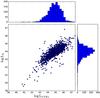 |
Fig. 1 Distribution of the measured UV and X-ray luminosities of our main sample. Both quantities are also plotted in histograms on the sides. Both luminosities are redshift corrected (see the main text for the details). |
2.3. Corona (power-law) luminosity
The corona (power-law) luminosity can be defined from the X-ray luminosity by extrapolating it to the energy interval 0.1−100 keV. Beyond these energy limits, the corona emission is usually diminished by low- and high-energy cut-offs. For the power-law luminosity, we can therefore write  (5)where DL is the luminosity distance constrained from the redshift measurement z, and F0.1−100 keV is the X-ray flux at the 0.1–100 keV energy calculated by an extrapolation of the observed 2–12 keV flux
 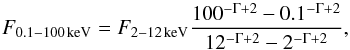 (6)where Γ is the photon index. The 100 keV threshold3 is selected to roughly correspond to an average value of the high-energy cut-off based on deep hard X-ray observations of type-1 AGN with INTEGRAL, Swift, and Nustar (Malizia et al. 2014; Fabian et al. 2015).
The photon index Γ can be constrained from the flux measurements in two neighbouring X-ray bands in the 3XMM catalogue. When calculating the photon index Γ, we assumed that the X-ray flux between energies Ea and Eb can be described as a power law:  (7)Using F0.5−2 keV and F2−12 keV we get for the photon index
 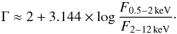 (8)We used the photon index as an indicator of a nature of the X-ray spectrum. While X-ray spectra that are too flat suggest a large effect of X-ray absorption, spectra that are too steep might be incompatible with AGN emission or suggest a low quality of the hard-band X-ray spectrum. Therefore, only sources with a photon index Γ in the interval 1.5 < Γ < 3.5 were considered in the sample creation. The mean value of the photon index of the main sample is Γmean = 1.7 ± 0.34. This value is consistent with reported values of the average photon index of unobscured AGN in the literature (Nandra & Pounds 1994; Steffen et al. 2006; Young et al. 2009; Liu et al. 2016).
2.4. Thermal disc luminosity
The thermal disc emission is characterised by a multi-colour black-body emission from accretion rings (Mitsuda et al. 1984), since the temperature decreases with the radius r, ![Mathematical equation: \begin{equation} T = \left[{\frac{3c^6}{4 \pi G^2 \sigma}\left({\frac{r}{r_{\rm g}}}\right)^{-3}\frac{\dot{M}}{M^2}}\right]^{\frac{1}{4}}, \end{equation}](/articles/aa/full_html/2017/07/aa30181-16/aa30181-16-eq56.png) (9)where
(9)where  is the gravitational radius, M is the black hole mass, Ṁ is the accretion rate, σ is the Stefan-Boltzmann constant, G is the gravitational constant, and c is the speed of light. The temperature at a given r in terms of rg is then inversely proportional to the one-fourth power of the black hole mass (assuming Ṁ ∝ M).
 ![Mathematical equation: \begin{equation} \label{temperature} T_{r[r_{\rm g}]} \propto M^{-\frac{1}{4}}. \end{equation}](/articles/aa/full_html/2017/07/aa30181-16/aa30181-16-eq64.png) (10)The characteristic peak temperature of the thermal emission is of the order of 1 keV (3 keV) for a non-rotating (highly rotating) stellar-mass black hole. This corresponds to 221 Å (73.6 Å) for a 106M⊙, and 1240 Å (413 Å) for a 109M⊙ supermassive black hole.
(10)The characteristic peak temperature of the thermal emission is of the order of 1 keV (3 keV) for a non-rotating (highly rotating) stellar-mass black hole. This corresponds to 221 Å (73.6 Å) for a 106M⊙, and 1240 Å (413 Å) for a 109M⊙ supermassive black hole.
For black hole mass less than 109M⊙ and spin a> 0, the rest-frame emission at longer wavelengths than 1240 Å always correspond to the rising part (in the energy domain) of the thermal disc emission and can be roughly approximated as a power law (therefore, we can use Eq. (2)). However, at wavelengths shorter then 1240 Å the emission might instead correspond to the high-energy tail of the thermal emission, and using a power-law approximation of the UV energy distribution would be invalid. Therefore, any measurements corresponding to rest-frame wavelengths shorter than 1240 Å were not considered.
For all sources of the main sample, we constrained the UV flux at the rest wavelength λref = 2910 Å, which is the mean wavelength of the UVW1 band. Owing to the cosmological redshift, different UV/optical filters might be closer to this rest-frame reference wavelength. The procedure to constrain the UV flux at the rest-frame reference wavelength was the following. First, we determined the rest-frame wavelengths of the mean wavelengths of all UV and optical filters on the Optical Monitor, UVW2 (2120 Å at z = 0), UVM2 (2310 Å at z = 0), UVW1 (2910 Å at z = 0), U (3440 Å at z = 0), B (4500 Å at z = 0), and V (5430 Å at z = 0). Then, we chose the two nearest filters to the rest-frame wavelength λref = 2910 Å, from which we constrained the UV spectral slope and the observed flux at the rest-frame wavelength. Finally, we multiplied the observed UV flux by a K-correction factor (1 + z) to get the intrinsic UV flux at the rest wavelength λref.
We used the redshift and Galactic extinction corrected UV flux to estimate the disc luminosity LD, which can be defined as  (11)where DL is the luminosity distance constrained from the redshift measurement z and A is an arbitrary factor, which can be chosen so that the sum of the disc and power-law luminosity, Ltot, roughly corresponds to the bolometric luminosity.
Therefore, we cross-correlated our sample with a sample of active galaxies studied by Vasudevan & Fabian (2009) who calculated the bolometric corrections from the simultaneous X-ray/UV and optical measurements by XMM-Newton. We obtained 13 sources present in both samples5. The multiplicative factor was constrained using the MPFIT procedure (Markwardt 2009) as A ≈ 2.4, with the standard deviation σA ≈ 0.6.
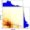 |
Fig. 2 Redshift-hardness distribution of the main sample. The coloured 2D histogram shows the number of sources in a particular bin of redshift and hardness interval. The inserted curves indicate the mean value (blue solid line), median value (blue dashed line), and the ratio of the median to mode (red dot-dashed line) of the hardness per redshift bin. The side-bar histograms show the total number of sources per hardness and redshift bins, respectively. |
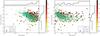 |
Fig. 3 Hardness-luminosity diagram for AGN. The coloured circles correspond to sources with constrained radio flux measurements, the colour denoting the relative radio loudness of the source. Radio-quiet sources, which have been detected only with an upper limit are shown by cyan triangles. The smaller green crosses correspond to sources with no available radio flux measurement. The side histograms show an average value of the relative radio-loudness in respective bins either in hardness (top) or luminosity (right). The histograms are calculated using only sources with constrained radio flux measurements. The plot is shown in logarithmic scale of hardness (left) for better comparison with XRBs and in linear scale (right) to show the hard-state part of the diagram in greater detail. |
2.5. Spectral hardness
The diagram showing the spectral hardness on one axis and the X-ray intensity on the other (the “Hardness-Intensity Diagram”) is widely used to track the spectral state evolution in black hole XRBs (Fender et al. 2004). For XRBs, the thermal emission and the hard X-ray emission are both measured in X-rays. However, as the thermal emission shifts to the UV energy band for AGN, the hardness needs to be defined between the UV and X-ray flux for AGN, for example as the ratio of the power-law luminosity against the total luminosity (sum of the power-law and disc luminosity):  (12)The redshift-hardness distribution of the main sample is shown in Fig. 2. Most of the sources are at the redshift z< 1.35 (see the upper panel of the figure). At higher redshifts, the UVW1 flux, which is the most commonly used filter in the Optical Monitor, corresponds to the rest-frame wavelength λ< 1240 Å. The sources at higher redshifts are included only if they have significant measurements in either optical band, U, B, or V. The highest concentration of the sources is at redshift around z ≈ 1 and hardness 0 <H< 0.3.
A mean (median) value of the hardness as a function of redshift is shown in Fig. 2 by a blue solid (dashed) line. The plot indicates that the average value of the hardness is always lower than 0.4. We note that the typical value of the hardness is significantly lower than a similar quantity in Koerding et al. (2006b) due to the different calculation of the disc and power-law luminosities. Figure 2 also reveals that the average hardness decreases with the redshift. However, this might be due to an observational bias, when at higher redshift more luminous sources usually in thermal (soft) states are observed. The red (dot-dashed) line shows the ratio of the median to mode (maximum value of the distribution in the given redshift interval). A large deviation of this curve from the median curve at high redshift indicates that the maximum value of the hardness at the high-redshift bins is much lower than for low-redshift intervals.
The radio loudness is defined as the ratio between the radio luminosity and the total luminosity:  (13)where 4.85 GHz corresponds to 6 cm wavelength. For sources, when the only available radio measurement is at 20 cm, the radio flux at 6 cm is estimated using Eq. (2). For practical purposes, we deal mainly with a relative radio loudness, calculated as the difference between the radio loudness and the minimal value of the radio loudness of the sample:
 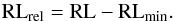 (14)
(14)
3. Results
3.1. Radio-loudness in the hardness-luminosity plane
The hardness-luminosity diagram for our main sample is shown in Fig. 3. Each source in the sample is represented by a point in the diagram. The sources with constrained radio flux measurements are emphasised by coloured circles whose colour corresponds to their relative radio loudness. Sources with no available radio flux measurements are marked by green crosses. Radio-quiet sources, marked as cyan triangles, are sources that were observed in radio surveys but only with an upper limit, which corresponds to the FIRST survey sensitivity limit (about 1 mJy). Such sources have a blank “nR” flag in the Véron catalogue.
The plot is shown in two versions using either a logarithmic or a linear hardness scale. The first (shown in the left panel) is more appropriate for comparison with XRBs, whose state diagrams are usually shown in logarithmic scale. The second plot shown in linear scale (right panel) reveals the hard-state part of the diagram in greater detail. It is apparent from the plots that the radio-quiet sources are on average softer with a relatively low hardness, which is less than 0.4 for most sources. In contrast, the sources with significant radio emission are spread over the hardness, and some of them appear in the upper right corner where radio-quiet sources are rarely represented.
The side-plot histograms show an average relative radio-loudness calculated per respective bin in hardness (top) and luminosity (right). Only sources with constrained radio flux measurements are used to compute these histograms. To avoid low-number statistics in the less populated parts of the diagram, we defined the bins to have an equal number of radio-loud sources in each bin.
The histogram reveals increasing radio loudness with hardness. We note that according to the definition of relative radio-loudness in Eq. (14), the increment of the average relative radio-loudness by one corresponds to an increase in the radio luminosity by one order of magnitude. The histogram of radio loudness as a function of luminosity reveals that the average radio loudness is higher for sources with high (log L> 46) and low (log L< 44) luminosities (but see how this changes for the Eddington ratio instead of luminosity, as shown in Fig. 8).
To quantify the statistical significance of the relation between radio loudness and hardness, we applied the Pearson statistical test, which gives the Pearson coefficient r = 0.246 and p-value p = 0.001. This result suggests a weak but statistically significant positive correlation. The statistical significance of this correlation is enhanced when low-luminosity sources are not included in the test (we also show that these sources might have hardness measurements which are systematically lower than their actual intrinsic values). For sources with the total luminosity log L> 44, the Pearson coefficient increases to r = 0.322 and the p-value decreases to p = 5 × 10⁻⁵, indicating that the radio loudness is higher for harder sources and lower for softer sources.
The low-luminosity radio-loud sources might correspond to analogous low-hard states in XRBs. They standardly populate the lower right corner of the diagram. However, their position in the AGN diagram, compared to the XRB one, is moved towards the left (which is especially apparent in the plot with the linear scale of hardness). The most likely explanation for this discrepancy is a significant contribution of a host galaxy that is unavoidable in low-luminosity sources and contributes more to UV than to X-rays. Consequently, the sources appear much softer in the hardness-luminosity diagram. In the most extreme case, when their AGN contribution is negligible in UV and their entire UV flux is due to the host galaxy, such sources would have intrinsically the greatest possible hardness, H = 1, but the “observed” hardness would be much lower.
3.2. Comparison with non-active galaxies
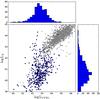 |
Fig. 4 Distribution of UV and X-ray fluxes measurements for non-active galaxies (dark blue). The distribution of AGN is overlaid (light grey). |
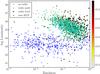 |
Fig. 5 Hardness-intensity diagram for non-active (blue crosses) and active galaxies (the same notation as in Fig. 3). |
To better understand the contribution of the host galaxy to the AGN UV spectrum, we performed a similar analysis to that done with AGN for galaxies that are considered to be inactive. The sample is created from the simultaneous XMM-Newton observations, as described in Sect. 2.1, by cross-correlation with the 2MASS catalogue of galaxies (Huchra et al. 2012). We removed all sources classified as quasars or AGN in the 2MASS catalogue, and also those sources which are present in our AGN sample. We also removed sources with undetected UV or X-ray (above 2 keV) flux, sources with an extended UV emission, and sources with zero or negative redshift. We applied correction on the Galactic reddening.
The distribution of measured UV and X-ray fluxes for the sample of non-active galaxies is shown in Fig. 4. The X-ray flux is significantly weaker with respect to the UV flux when compared to AGN, which are overlaid in the plot and denoted by light grey dots. Some of the sources with high X-ray luminosity probably contain a hidden active nucleus because the X-ray luminosity due to starlight in the host galaxy can hardly exceed log LX ≈ 42 (Gilfanov & Merloni 2014). While their X-ray luminosity exceeds the possible contribution of the host galaxy, the UV luminosity can still be entirely due to the host galaxy, since the host-galaxy UV contribution peaks at log LUV,host−galaxy ≲ 43.
Figure 5 shows the hardness-luminosity diagram for both non-active and active galaxies together. The disc and power-law luminosity of non-active galaxies are calculated in a similar but simpler way, as proportional to UV and X-ray luminosity (Ldisc ≈ 2 × LUVW1, and Lpower−law ≈ 10 × L2−10keV) for all sources. The plot is shown in a logarithmic scale in the hardness for better clarity. The plot reveals that the non-active galaxies appear very soft, which is the consequence of the significantly larger contribution of the host galaxy in UV than in the X-ray domain.
In general, the level of mixing of AGN with non-active galaxies is very low in Fig. 5. However, some non-active galaxies in our sample exhibit a luminosity exceeding log Ltot ≈ 43, where low-luminosity AGN appear. This implies that the apparent softness of low-luminosity AGN (log L< 44) may indeed be due to the contribution of the host galaxy. Therefore, for these sources it is essential to correctly estimate the host-galaxy contribution. However, the effect due to the host-galaxy contamination is not easy to estimate from the available data; a possible treatment will be discussed in Sect. 4.2.
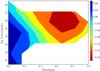 |
Fig. 6 Distribution of the photon index difference ΔΓ = Γ−Γmean (indicated by colour) of the whole sample in the hardness-luminosity diagram. Negative values correspond to harder X-ray spectra and positive values to softer ones. |
3.3. UV and X-ray spectral slope in the hardness-luminosity plane
Higher sensitivity of the X-ray and UV measurements by XMM-Newton allows us to construct hardness-luminosity diagrams, which – instead of radio loudness – show the X-ray hardness and UV slope, respectively. To have a more detailed look at the hard-state part of the diagram, we use the linear scale of the hardness in these plots. Because there are a relatively large number of sources with measured X-ray and UV slopes, we show these plots using coloured contours instead of scatter plots. Figure 6 shows the relative difference of the X-ray photon index with respect to its average value: ΔΓ = Γ−Γmean. Negative values of ΔΓ (red) correspond to lower values of the photon index and thus flatter X-ray spectra. The locations of these sources in the diagram are consistent with the expected location of sources in the hard state.
Similarly, Fig. 7 shows the relative difference in the UV slope, defined as Δβ = β−βmean. Only sources with measured UV slopes are used for this plot. The UV slope is calculated in the wavelength domain and thus the positive value (red) corresponds to a flatter spectrum. Steeper spectra are characteristic of the disc thermal emission, while flat UV spectra indicate that the UV emission might be dominated by other spectral components. Flat UV spectra are especially found at low-luminosity sources, which might indicate a large effect of the host galaxy contribution there.
3.4. XMM-SDSS subsample
A significant part of our sample has complementary measurements in the optical domain from the Sloan Digital Sky Survey (SDSS; Gunn et al. 2006). For sources from the 7th SDSS data release, Shen et al. (2011) also constrained the black hole mass, which may be used to scale the luminosity to the Eddington luminosity. As the Eddington ratio better corresponds to the real accretion state than the total luminosity, especially given that our sample spans a wide range in the black hole mass, we decided to use only the 316 sources sources with measured black hole mass. We note that the mass estimates are the virial masses, which may be discrepant from the true black hole masses (see Shen et al. 2011 for a more detailed discussion), but they are the best available estimates we have for our analysis (see also Sect. 4.4).
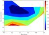 |
Fig. 7 Distribution of the UV slope difference Δβ = β−βmean (indicated by colour) in the hardness-luminosity diagram . Only sources with measured UV slope from the XMM-Newton Optical Monitor are considered. |
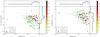 |
Fig. 8 Radio-loudness in the hardness-luminosity (left) and the hardness-Eddington ratio (right) diagram for sources of the XMM-SDSS subsample. |
Figure 8 shows the radio-loudness in the hardness versus luminosity plot (left panel) and versus the Eddington ratio (right panel) for the XMM-SDSS subsample. Both plots show a higher concentration of radio-loud sources in the harder part of the diagram. However, the vertical positions of several sources significantly change between the plots. The luminosity plot shows that the radio-loud sources are on average more luminous than the radio-quiet sources. On the other hand, the distribution of the Eddington ratios between radio-quiet and radio-loud sources is comparable. The average radio-loudness is stronger for lower-accreting sources, while it decreases when the accretion rate approaches the Eddington limit.
Sources at the low Eddington ratio are clearly harder than most sources in the sample. An average value of the hardness is HSDSS,mean ≈ 0.25 for the whole subsample, while for the low Eddington ratio sources (λEdd< −1.4) the hardness is HlowEdd. ≈ 0.5. The XMM-SDSS subsample does not contain any sources whose luminosity is lower than log Ltot ≈ 44, and thus the effect of a host galaxy is not prominent in this sample. The diagram with the Eddington ratio is more reminiscent of the analogous diagram for XRBs, indicating that the Eddington ratio is a more appropriate proxy of the accretion rate.
4. Discussion
4.1. Similarity of the AGN and XRB spectral-state evolutionary diagrams
The AGN hardness-luminosity diagrams (Figs. 3 and 8) can be qualitatively compared with an analogous diagram created for a sample of XRBs (e.g. Fig. 8 of Dunn et al. 2010). The global appearance is quite similar for sources above log Ltot> 44. Radio-loud sources concentrated towards the right part of the hardness-luminosity diagram indicate that jets are launched when the sources are in the hard states characterised by a higher ratio between the X-ray and UV emission, harder X-ray spectra, and flatter UV spectra. In contrast, the jets seem to be almost absent in the soft states (upper left part of the state diagrams), when the sources are characterised by a much stronger UV bump due to the thermal disc emission and softer X-ray spectral slope, confirming the long-held belief that most luminous AGN are indeed radio quiet.
A remarkable difference between our AGN (Fig. 3) and XRB diagrams was found in the low-luminosity range. Low-luminosity AGN are softer than the low-hard state analogies would be in the hardness-luminosity diagram. The most likely explanation for this difference is a significant contribution of the host galaxy to the UV flux. This “galaxy dilution” problem is well known in surveys selecting AGN via their optical/UV emission (see e.g. Merloni 2016), and is the most severe limitation when attempting to characterise genuine analogues of the low-hard state in AGN samples. A proper decomposition of the nuclear and host-galaxy contribution is therefore crucial to correctly place the low-luminosity sources in the diagram, and we discuss this in the following section.
4.2. Host galaxy contamination
In the absence of very high spatial resolution observations, available only for the nearest galaxies, the only reliable deconvolution of the host galaxy contamination is obtained by a detailed modelling of the AGN SED (see e.g. Ho 1999, 2008, and references therein). This has been done so far for only nearby low-luminosity AGN, and there is not yet a fully accepted consensus on the UV emission of a special class of low-luminosity AGN, the LINERs. While Ho (2008) concluded that these sources completely lack the UV emission from the nucleus, Maoz (2007) found a significant contribution that can be associated with the nuclear activity.
In the first case, where all UV flux is from the star light, the affected sources should be moved entirely to the right in the diagram (the hardness would be equal to one). For the second case, we can compare the results by Maoz (2007) with the measurements of our final sample. However, the only source from his study that fulfils our strict filtering criteria for creating the final sample is NGC 3998. Its hardness from the analysis by Maoz (2007) is HMaoz, NGC 3998 = 0.86. The hardness from our main sample without any host-galaxy correction is HNGC 3998 = 0.21 ± 0.01, which is significantly lower. This clearly indicates that the disc luminosity is largely overestimated in such sources.
A detailed analysis of the host-galaxy contribution of all low-luminosity sources in our sample is beyond the scope of this paper. However, we could use some empirical relations to estimate its contribution. One possibility would be to use the mean values of the UV and X-ray flux measurements of non-active galaxies shown in Fig. 4. However, the AGN hosts may be even brighter since the nuclear activity may be related to the enhanced star formation, as shown by, e.g., Vanden Berk et al. (2005) and Santini et al. (2012). Subtracting an average host-galaxy contribution based on non-active galaxies might therefore be insufficient.
A tight correlation between the emission of the host galaxy and bolometric AGN luminosity was found by Netzer (2009). Therefore, we used the relation obtained from their Fig. 13 to estimate the star-formation luminosity as  (15)where LSFR = νLν,60 μm is the infrared luminosity measured at 60 micrometres, and Lbol is the bolometric luminosity.
We used the total luminosity Ltot (= Ldisc + Lpower−law) as an approximate estimate of the bolometric luminosity. We further constrain the star formation rate (SFR) using the relation by Calzetti et al. (2010)6:  (16)The UV luminosity can be then estimated from the SFR using a relation based on GALEX NUV data (Murphy et al. 2011; Hao et al. 2011; Kennicutt & Evans 2012):
  (17)Because the average frequency of the UVW1 and GALEX-NUV bands differ, we multiplied the obtained UV luminosity by the ratio between these frequencies (i.e. by a factor 2301/2910 ≈ 0.79) to estimate the contribution of the host galaxy in LUVW1.
Similarly, we can estimate the X-ray luminosity from the SFR (Gilfanov & Merloni 2014; Mineo et al. 2014). We used the relation by Gilfanov & Merloni (2014):  (18)Figure 9 shows the hardness-luminosity diagram after the applied host-galaxy correction using Eqs. (17) and (18). The plot is shown in the linear scale for hardness to focus on changes in the hard part of the diagram, and can therefore be directly compared to the right panel of Fig. 3. The radio-loud sources moved to the right in the diagram, towards higher hardness as expected. For NGC 3998, we get a “corrected” value of the hardness HNGC 3998 = 0.48 ± 0.01, which is, however, still insufficient.
 |
Fig. 9 Hardness-luminosity diagram with applied host-galaxy correction according to Eqs. (17) and (18). The notation is the same as in Fig. 3. The side histograms show an average value of the relative radio-loudness in respective bins either in hardness (top) or luminosity (right). |
We note that while the detailed spectral decomposition would be the best way to treat the low-luminosity sources, several indirect methods can be employed in future extensions of current work. One way to estimate the intrinsic UV emission of low-luminosity sources is from the broad H-alpha luminosity (Stern & Laor 2012), i.e. from the reprocessing of the central flux in the broad-line region. Intrinsic luminosities can also be estimated from the reprocessed emission at the torus, which is observed in the mid-IR band. This emission is closely related to the intrinsic emission from the central AGN (Asmus et al. 2015). However, the spectral energy decomposition of a large sample of AGN with deep multi-wavelength observations is clearly the most reliable way.
4.3. Effect of the intrinsic reddening on measured UV slopes
Not only hardness might be affected by the host galaxy, but also the measured UV slope. The UV slope shown in the binned AGN hardness-luminosity diagram (Fig. 7) was calculated according to Eq. (4) and was corrected for the Galactic extinction. However, it was not corrected for an intrinsic extinction due to the host galaxy.
The intrinsic extinction could be estimated as in Eq. (1). However, the ratio of the total to selective extinction RV typically has a different shape than the Galactic profile (see e.g. Calzetti et al. 1994; Richards et al. 2003; Gaskell & Benker 2007). Based on the SDSS quasar extinction measurements by Richards et al. (2003), Czerny et al. (2004) derived a simple empirical formula, 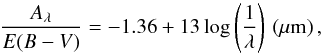 (19)valid in the range of (1 /λ) between 1.5 and 8.5 (μm)-1.
We used this formula to estimate extinction at UVW1 (2910 Å), UVM2 (2310 Å), and UVW2 (2120 Å) wavelengths. We get A2910 Å = 5.6, A2310 Å = 6.9, and A2120 Å = 7.4, respectively. For the difference in the measured and intrinsic UV slope between the UVW1 and UVM2 bands, we obtained  (20)The difference in the UV slope is thus linearly proportional to the intrinsic reddening. For high intrinsic reddening, E(B−V) ≳ 0.1, the UV slope difference between the intrinsic and measured value is ΔβUVW1−UVM2 ≳ 0.5. However, for a typical intrinsic reddening of quasars, Gaskell et al. (2004) concluded that more than 90 % of the SDSS quasar sample has intrinsic reddening E(B−V) < 0.055 (see also Vasudevan & Fabian 2007; Lusso et al. 2010). This corresponds to ΔβUVW1−UVM2 ≈ 0.25, which is smaller than the distribution of uncorrected UV slopes (see Fig. 7). However, the intrinsic reddening might be significantly higher in the case of low-luminosity sources, for which a more robust analysis is needed to estimate the effect of the intrinsic reddening, and this should be investigated in future work.
 |
Fig. 10 Comparison of the mass measurements from the X-ray variability by Ponti et al. (2012) with the virial mass constraints from Shen et al. (2011). The dashed line represents the 1:1 ratio, showing that the methods are in very good agreement. |
4.4. Mass and hardness-ratio (Eddington) diagrams
A significant uncertainty in the hardness-luminosity diagrams for AGN is the mass of the central black hole. The range of possible masses is large, in extremes from 105 to 1010 solar masses. Therefore, a more appropriate quantity than the luminosity is the luminosity scaled by the black hole mass, i.e. the Eddington ratio. The most reliable method for determining mass, the reverberation technique (Peterson et al. 2004), has been applied only to a small sample of local AGN. Therefore, the black hole mass in AGN is usually constrained from empirical correlations between the mass and the luminosity of a specific emission line or the continuum flux density at a specific wavelength in the optical band; however, it is affected by a large uncertainty (see e.g. Denney et al. 2009).
Another possible technique to constrain the black hole mass is through X-ray variability (Zhou et al. 2010; Ponti et al. 2012). Although some information about the X-ray variability is reported in the most recent release of the 3XMM catalogue, there are several reasons why this information cannot be directly used. First, the reported values correspond to maximal variability detected over the exposure, and so the real variability is, in general, lower. Second, the variability measurements are sensitive to high background-flare events that need to be omitted from the light curve used for the calculations. Last, we found that the reported values are often not consistent between different detectors (PN and MOS). Therefore, the light curves would need to be properly analysed in detail, which is beyond the scope of this paper.
Instead, we used the virial black hole mass measurements from the SDSS catalogue (Shen et al. 2011). The estimates are done on the width of Hα, Hβ, Mg II, and C IV emission lines. Although these measurements might be affected by systematic uncertainties (unavoidable in the conversion between the line luminosity and the mass or bolometric luminosity), we found that there is a quite good agreement of measured masses for sources with the mass constrained from the X-ray variability (see Fig. 10).
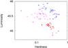 |
Fig. 11 Hardness-luminosity diagram for three sources with the largest number of observations available in the XMM-Newton catalogue: CDFS J03321-2747 (red), CDFS J03324-2741B (blue), CDFS J03324-2740 (magenta). The crosses represent the simultaneous data, while the open circles show the extreme values of any possible combinations of UV and X-ray fluxes. |
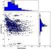 |
Fig. 12 Hardness-luminosity diagram for sources with multiple observations available in the XMM-Newton catalogue. The blue points represent all simultaneous UV and X-ray observations, while the grey points represent all possible combinations of measured UV and X-ray flux for each source with multiple observations. The side-plot histograms show fractional distribution (in percent) of the hardness and luminosity for simultaneous measurements (blue boxes) and all possible combined measurements (grey boxes), respectively. |
4.5. Variability of source positions in the hardness-luminosity diagrams and effects of non-simultaneity
Thanks to the simultaneity of the UV and X-ray observations by XMM-Newton, in our analysis we can rule out any effects of source variability when observations from different epochs are compared. However, the UV and X-ray emission are not supposed to originate at exactly the same region. While the X-rays are believed to come from a more central region (X-ray corona, X-ray reflection at the innermost accretion disc), the UV flux may be dominated by emission coming from more distant parts of the accretion disc. Thus, despite the simultaneity of observations, some variability of source positions in the hardness-luminosity diagrams can still be expected in both hardness and luminosity. Therefore, we further investigate the variability of source positions in the diagram for sources with multiple observations available.
Figure 11 shows the hardness-luminosity diagram for three sources with the highest number of different observations in the XMM-Newton catalogue. The hardness and luminosity constrained from the simultaneously measured UV and X-ray fluxes are shown by crosses, while the open circles show the extreme values obtained from any possible combination of measured UV and X-ray flux without requiring its simultaneity. The lowest hardness is obtained when the minimum X-ray and maximum UV flux are combined, and vice versa for the highest hardness. Similarly for luminosity, the highest value is obtained by a combination of maximum values of measured fluxes and the lowest from minimum ones. The plot shows a quite large scatter in the hardness-luminosity diagram position even for simultaneous data. The extreme values obtained by a combination of (non-simultaneously) measured minimum and maximum values of UV and X-ray fluxes are not largely offset from the simultaneous data. This clearly illustrates that the scatter in the hardness-luminosity relation is not dominated by the non-simultaneity of the data, but rather by some intrinsic variability of the accretion-disc corona system.
The luminosity-hardness plane for all sources with available multiple observations in the XMM-Newton catalogue is shown in Fig. 12. The simultaneous measurements (blue points) are overlaid on all possible combinations of their non-simultaneous measurements (grey points). The side-plot histograms show the fractional distribution of different values of hardness and luminosity. Because the distributions are not very different, a strict simultaneity of UV and X-ray measurements is not critical in this kind of analysis. This is consistent with a similar conclusion made by Vagnetti et al. (2010), who analysed αox distribution of the AGN observations by XMM-Newton. They also realised that the intrinsic variability is significantly greater than any artificial variability caused by non-simultaneity.
4.6. Sample selection and biases
We have shown the AGN state diagrams for a sample of bona fide identified AGN in the XMM-Newton EPIC and OM serendipitous source catalogues. We excluded blazars, whose X-ray emission is dominated by a relativistically boosted radiation from collimated jets, extended sources, and also heavily X-ray obscured sources where no direct X-ray emission from the nuclear region is expected to be detected. The advantage of the sample is that it contains a large number of sources sensitively and simultaneously measured in the UV and X-ray bands by the same satellite.
Still, the sample is not homogeneous enough to be directly used to investigate the source density in different parts of the diagram and compare it with XRBs, for which this quantity was constrained by Dunn et al. (2010). Deep and wide surveys are necessary to have a more homogeneous sample. The main advantage of such surveys is the availability of multi-wavelength measurements, which allow a more detailed analysis, in particular to properly calculate the UV de-reddening and contribution of the host galaxies. This is most critical for low-luminosity sources, which are, however, not well represented in the existing samples. Therefore, even deeper and more sensitive surveys are needed to significantly improve the analysis done in this paper.
The next X-ray missions, such as e-ROSITA (Predehl et al. 2014) or Athena (Nandra et al. 2013), will provide data with the required sensitivity, as will the planned radio facilities, such as ASKAP/EMU in the southern hemisphere or APERITIF/WODAN in the north (for a review see e.g. Norris et al. 2013), and finally the SKA radio interferometer (Dewdney et al. 2009) will significantly increase the sensitivity of the radio measurements.
5. Conclusions
We studied the analogy between the accreting black holes in XRBs and active galactic nuclei by investigating the spectral states of AGN and their relation to the radio properties. We employed simultaneous UV and X-ray observations of AGN performed by the XMM-Newton satellite in the period 2000-13 to compare their total luminosity with hardness, defined as the ratio of the X-ray power-law luminosity against the total luminosity composed of thermal disc emission, as well as the non-thermal corona X-ray emission.
We found that radio loudness increases on average with hardness, suggesting that the jet emission occurs in the hard accretion states, consistently with XRBs and with previous results obtained by Koerding et al. (2006b) using non-simultaneous measurements of quasars. By analysis of sources with multiple observations, we realised that the scatter in the hardness-luminosity relation is not dominated by the non-simultaneity of the data, but rather by some intrinsic variability of the accretion-disc corona system.
The high sensitivity of the detectors on board the XMM-Newton satellite also allowed us to study low-luminosity sources (log Ltot< 44). However, we found that especially their UV emission is strongly affected by their host-galaxy contamination, leading to a significant underestimate of the hardness. A more detailed spectral decomposition is needed to properly constrain the intrinsic luminosity of such sources.
We showed the AGN state diagrams for a subsample of sources that were present in the SDSS survey and for which virial black hole mass estimates were available. The Eddington ratio calculated from the black hole mass is more appropriate for characterising the accretion state than the total luminosity. The hardness-Eddington ratio diagram revealed that the average radio-loudness is higher for low-accreting sources, while it decreases when the accretion rate is close to the Eddington limit.
A significant improvement in our analysis can be achieved with more sensitive multi-wavelength observational surveys. The three most important aspects are the precise measurements of the radio, UV, and X-ray intrinsic luminosities properly corrected for the host-galaxy contamination; the large size and homogeneity of the sample; and the reliable mass measurements of central supermassive black holes.
We never used the UV flux measurements corresponding to the rest-frame wavelength shorter than λcrit = 1240 Å, which is explained in greater detail in Sect. 2.4.
The uncertainty of the total X-ray flux is of the order of 10% assuming the photon index Γ = 1.7 and the high-energy cut-off that varies between 60 and 300 keV.
We also constrained the hard X-ray photon index from the energy intervals 2−4.5 keV and 4.5−12 keV, as 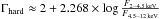 , which has the advantage of avoiding the contamination by the soft X-ray absorption. Its average value is consistent with the broad-band value Γhard = 1.7 ± 0.8, but has a much larger dispersion, indicating a larger scatter, which might be due to a lower signal-to-noise ratio in the narrower hard bands. Therefore, we used only the broad-band value of the X-ray photon index as defined from the 0.5−2 keV and 2−12 keV energy bands.
3C 390.3, Mrk 110, PG 0953+414, PG 1226+023, FAIRALL9, 3C 120, Mrk 1095, Mrk 590, Mrk 79, NGC 5548, NGC 7469, PG 0052+251, PG 2130+099.
LSFR is constrained from the infrared luminosity νLν,70 μm at 70 μm in the relation by Calzetti et al. (2010), but we made an assumption that within the general uncertainties we can assume that the infrared spectrum between these two bands is relatively flat (see e.g. Symeonidis et al. 2016).
Acknowledgments
The authors thank the anonymous referee for the helpful suggestions and comments that led to a significant improvement of this work. J.S. also acknowledges very useful discussions with Ignacio de la Calle, Giovanni Miniutti, Sara Elisa Motta, Margherita Giustini, Gabriele Ponti, Barbara de Marco, Marion Cadolle Bel, Erin Kara, and Victoria Grinberg. This research was financially supported from the Grant Agency of the Czech Republic within the project No. 14-20970P. The research was also partially funded by the European Union Seventh Framework Program (FP7/2007−2013) under grant 312789. The presented work is based on observations obtained with XMM-Newton, an ESA science mission with instruments and contributions directly funded by ESA Member States and NASA.
References
- Ade, P. A. R., Aghanim, N., Arnaud, M., et al. 2016, A&A, 594, A13 [NASA ADS] [CrossRef] [EDP Sciences] [Google Scholar]
- Adelman-McCarthy, J., Agüeros, M., Allam, S., et al. 2006, ApJS, 162, 38 [NASA ADS] [CrossRef] [Google Scholar]
- Alam, S., Albareti, F. D., Prieto, C. A., et al. 2015, ApJS, 219, 12 [NASA ADS] [CrossRef] [Google Scholar]
- Asmus, D., Gandhi, P., Hönig, S. F., Smette, A., & Duschl, W. J. 2015, MNRAS, 454, 766 [NASA ADS] [CrossRef] [Google Scholar]
- Ballo, L., Giustini, M., Schartel, N., et al. 2008, A&A, 483, 137 [NASA ADS] [CrossRef] [EDP Sciences] [Google Scholar]
- Becker, R. H., White, R. L., & Helfand, D. J. 1995, ApJ, 450, 559 [NASA ADS] [CrossRef] [Google Scholar]
- Bianchi, S., Piconcelli, E., Chiaberge, M., et al. 2009, ApJ, 695, 781 [NASA ADS] [CrossRef] [Google Scholar]
- Blandford, R., & Znajek, R. 1977, MNRAS, 179, 433 [Google Scholar]
- Bolton, A. S., Schlegel, D. J., Aubourg, É., et al. 2012, AJ, 144, 144 [NASA ADS] [CrossRef] [Google Scholar]
- Calzetti, D., Kinney, A. L., & Storchi-Bergmann, T. 1994, ApJ, 429, 582 [NASA ADS] [CrossRef] [Google Scholar]
- Calzetti, D., Wu, S.-Y., Hong, S., et al. 2010, ApJ, 714, 1256 [NASA ADS] [CrossRef] [Google Scholar]
- Condon, J. J., Cotton, W. D., Greisen, E. W., et al. 1998, AJ, 115, 1693 [NASA ADS] [CrossRef] [Google Scholar]
- Czerny, B., Li, J., Loska, Z., & Szczerba, R. 2004, MNRAS, 348, L54 [NASA ADS] [CrossRef] [Google Scholar]
- Denney, K. D., Peterson, B. M., Dietrich, M., Vestergaard, M., & Bentz, M. C. 2009, ApJ, 692, 246 [NASA ADS] [CrossRef] [Google Scholar]
- Dewdney, P., Hall, P., Schilizzi, R., & Lazio, T. 2009, Proc. IEEE, 97, 1482 [NASA ADS] [CrossRef] [Google Scholar]
- Done, C. 2014, in Suzaku-MAXI 2014: Expanding the Frontiers of the X-ray Universe, eds. M. Ishida, R. Petre, & K. Mitsuda, Conf. Proc., 300 [Google Scholar]
- Done, C., Gierliński, M., & Kubota, A. 2007, A&ARv, 15, 1 [NASA ADS] [CrossRef] [EDP Sciences] [Google Scholar]
- Done, C., Davis, S. W., Jin, C., Blaes, O., & Ward, M. 2012, MNRAS, 420, 1848 [NASA ADS] [CrossRef] [Google Scholar]
- Dunn, R. J. H., Fender, R. P., Körding, E. G., Belloni, T., & Cabanac, C. 2010, MNRAS, 403, 61 [NASA ADS] [CrossRef] [Google Scholar]
- Elvis, M., Wilkes, B. J., McDowell, J. C., et al. 1994, ApJS, 95, 1 [NASA ADS] [CrossRef] [Google Scholar]
- Elvis, M., Risaliti, G., Nicastro, F., et al. 2004, ApJ, 615, L25 [NASA ADS] [CrossRef] [Google Scholar]
- Esin, A., McClintock, J., & Narayan, R. 1997, ApJ, 489, 865 [NASA ADS] [CrossRef] [Google Scholar]
- Fabian, A. C., Lohfink, A., Kara, E., et al. 2015, MNRAS, 451, 4375 [NASA ADS] [CrossRef] [Google Scholar]
- Falcke, H., Koerding, E. G., & Markoff, S. 2004, A&A, 414, 895 [NASA ADS] [CrossRef] [EDP Sciences] [Google Scholar]
- Fender, R., & Belloni, T. 2012, Science, 337, 540 [NASA ADS] [CrossRef] [PubMed] [Google Scholar]
- Fender, R. P., Belloni, T. M., & Gallo, E. 2004, MNRAS, 355, 1105 [NASA ADS] [CrossRef] [Google Scholar]
- Fender, R. P., Homan, J., & Belloni, T. 2009, MNRAS, 396, 1370 [NASA ADS] [CrossRef] [Google Scholar]
- Fitzpatrick, E. 1999, PASP, 111, 63 [NASA ADS] [CrossRef] [Google Scholar]
- Gaskell, C. M., & Benker, A. J. 2007, ArXiv e-prints [arXiv:0711.1013] [Google Scholar]
- Gaskell, C. M., Goosmann, R. W., Antonucci, R., & Whysong, D. H. 2004, ApJ, 616, 147 [NASA ADS] [CrossRef] [Google Scholar]
- Gilfanov, M., & Merloni, A. 2014, Space Sci. Rev., 183, 121 [NASA ADS] [CrossRef] [Google Scholar]
- Gunn, J. E., Siegmund, W. A., Mannery, E. J., et al. 2006, AJ, 131, 2332 [NASA ADS] [CrossRef] [Google Scholar]
- Güver, T., & Özel, F. 2009, MNRAS, 400, 2050 [NASA ADS] [CrossRef] [Google Scholar]
- Hao, C.-N., Kennicutt, R. C., Johnson, B. D., et al. 2011, ApJ, 741, 124 [NASA ADS] [CrossRef] [Google Scholar]
- Hasinger, G., Cappelluti, N., Brunner, H., et al. 2007, ApJS, 172, 29 [NASA ADS] [CrossRef] [Google Scholar]
- Ho, L. C. 1999, ApJ, 516, 34 [Google Scholar]
- Ho, L. C. 2008, ARA&A, 46, 475 [NASA ADS] [CrossRef] [Google Scholar]
- Ho, L. C., & Ulvestad, J. S. 2001, ApJS, 133, 77 [NASA ADS] [CrossRef] [Google Scholar]
- Huchra, J. P., Macri, L. M., Masters, K. L., et al. 2012, ApJS, 199, 26 [NASA ADS] [CrossRef] [Google Scholar]
- Kalberla, P. M. W., Burton, W. B., Hartmann, D., et al. 2005, A&A, 440, 9 [Google Scholar]
- Kellermann, K. I., Sramek, R., Schmidt, M., Shaffer, D. B., & Green, R. 1989, AJ, 98, 1195 [NASA ADS] [CrossRef] [Google Scholar]
- Kennicutt, R. C., & Evans, N. J. 2012, ARA&A, 50, 531 [NASA ADS] [CrossRef] [Google Scholar]
- Koerding, E. G., Falcke, H., & Corbel, S. 2006a, A&A, 456, 439 [NASA ADS] [CrossRef] [EDP Sciences] [Google Scholar]
- Koerding, E. G., Jester, S., & Fender, R. P. 2006b, MNRAS, 372, 1366 [NASA ADS] [CrossRef] [Google Scholar]
- LaMassa, S. M., Cales, S., Moran, E. C., et al. 2015, ApJ, 800, 144 [NASA ADS] [CrossRef] [Google Scholar]
- Laor, A., & Netzer, H. 1989, MNRAS, 238, 897 [NASA ADS] [CrossRef] [Google Scholar]
- Liu, Z., Merloni, A., Georgakakis, A., et al. 2016, MNRAS, 459, 1602 [NASA ADS] [CrossRef] [Google Scholar]
- Lusso, E., Comastri, A., Vignali, C., et al. 2010, A&A, 512, A34 [NASA ADS] [CrossRef] [EDP Sciences] [Google Scholar]
- Lusso, E., Comastri, A., Simmons, B. D., et al. 2012, MNRAS, 425, 623 [NASA ADS] [CrossRef] [Google Scholar]
- MacLeod, C. L., Ross, N. P., Lawrence, A., et al. 2016, MNRAS, 457, 389 [NASA ADS] [CrossRef] [Google Scholar]
- Malizia, A., Molina, M., Bassani, L., et al. 2014, ApJ, 782, L25 [NASA ADS] [CrossRef] [Google Scholar]
- Malkan, M. A., & Sargent, W. L. W. 1982, ApJ, 254, 22 [NASA ADS] [CrossRef] [Google Scholar]
- Maoz, D. 2007, MNRAS, 377, 1696 [NASA ADS] [CrossRef] [Google Scholar]
- Markwardt, C. 2009, Astronomical Data Analysis Software and Systems XVIII, ASP Conf. Ser., 411 [Google Scholar]
- McElroy, R. E., Husemann, B., Croom, S. M., et al. 2016, A&A, 593, L8 [NASA ADS] [CrossRef] [EDP Sciences] [Google Scholar]
- McHardy, I. M., Koerding, E. G., Knigge, C., Uttley, P., & Fender, R. P. 2006, Nature, 444, 10 [Google Scholar]
- Merloni, A. 2016, Lect. Notes Phys., 905, 101 [NASA ADS] [CrossRef] [Google Scholar]
- Merloni, A., & Heinz, S. 2008, MNRAS, 388, 1011 [NASA ADS] [Google Scholar]
- Merloni, A., Heinz, S., & Di Matteo, T. 2003, MNRAS, 345, 21 [Google Scholar]
- Merloni, A., Dwelly, T., Salvato, M., et al. 2015, MNRAS, 452, 69 [NASA ADS] [CrossRef] [Google Scholar]
- Mineo, S., Gilfanov, M., Lehmer, B. D., Morrison, G. E., & Sunyaev, R. 2014, MNRAS, 437, 1698 [NASA ADS] [CrossRef] [Google Scholar]
- Miniutti, G., Sanfrutos, M., Beuchert, T., et al. 2014, MNRAS, 437, 1776 [NASA ADS] [CrossRef] [PubMed] [Google Scholar]
- Mitsuda, K., Inoue, H., Koyama, K., et al. 1984, PASJ, 36, 741 [NASA ADS] [Google Scholar]
- Murphy, E. J., Condon, J. J., Schinnerer, E., et al. 2011, ApJ, 737, 67 [NASA ADS] [CrossRef] [Google Scholar]
- Nandra, K., & Pounds, K. A. 1994, MNRAS, 268, 405 [NASA ADS] [CrossRef] [Google Scholar]
- Nandra, K., Barret, D., Barcons, X., et al. 2013, ArXiv e-prints [arXiv:1306.2307] [Google Scholar]
- Narayan, R., & McClintock, J. E. 2012, MNRAS, 419, L69 [NASA ADS] [CrossRef] [Google Scholar]
- Netzer, H. 2009, MNRAS, 399, 1907 [NASA ADS] [CrossRef] [Google Scholar]
- Netzer, H. 2015, ARA&A, 53, 365 [NASA ADS] [CrossRef] [Google Scholar]
- Norris, R. P., Afonso, J., Bacon, D., et al. 2013, PASA, 30, 54 [Google Scholar]
- Page, M., Brindle, C., Talavera, A., et al. 2012, MNRAS, 426, 903 [Google Scholar]
- Peterson, B. M., Ferrarese, L., Gilbert, K. M., et al. 2004, ApJ, 613, 682 [NASA ADS] [CrossRef] [Google Scholar]
- Ponti, G., Papadakis, I., Bianchi, S., et al. 2012, A&A, 542, A83 [NASA ADS] [CrossRef] [EDP Sciences] [Google Scholar]
- Predehl, P., Andritschke, R., Becker, W., et al. 2014, in Proc. SPIE 9144, eds. T. Takahashi, J.-W. A. den Herder, & M. Bautz, 91441T [Google Scholar]
- Puccetti, S., Fiore, F., Risaliti, G., et al. 2007, MNRAS, 377, 607 [NASA ADS] [CrossRef] [Google Scholar]
- Remillard, R., & McClintock, J. 2006, ARA&A, 44, 49 [NASA ADS] [CrossRef] [Google Scholar]
- Richards, G. T., Hall, P. B., Vanden Berk, D. E., et al. 2003, AJ, 126, 1131 [NASA ADS] [CrossRef] [Google Scholar]
- Richards, G., Lacy, M., Storrie-lombardi, L. J., et al. 2006, ApJS, 470 [Google Scholar]
- Risaliti, G., Elvis, M., & Nicastro, F. 2002, ApJ, 571, 234 [NASA ADS] [CrossRef] [Google Scholar]
- Risaliti, G., Elvis, M., Fabbiano, G., Baldi, A., & Zezas, A. 2005, ApJ, 623, L93 [NASA ADS] [CrossRef] [Google Scholar]
- Rosen, S. R., Webb, N. A., Watson, M. G., et al. 2016, A&A, 590, A1 [NASA ADS] [CrossRef] [EDP Sciences] [Google Scholar]
- Santini, P., Rosario, D. J., Shao, L., et al. 2012, A&A, 540, A109 [NASA ADS] [CrossRef] [EDP Sciences] [Google Scholar]
- Savage, B. D., & Mathis, J. S. 1979, ARA&A, 17, 73 [NASA ADS] [CrossRef] [Google Scholar]
- Schawinski, K., Koss, M., Berney, S., & Sartori, L. 2015, MNRAS, 451, 2517 [NASA ADS] [CrossRef] [Google Scholar]
- Scott, J. E., Kriss, G. A., Brotherton, M., et al. 2004, ApJ, 615, 135 [NASA ADS] [CrossRef] [Google Scholar]
- Scoville, N., Aussel, H., Brusa, M., et al. 2007, ApJS, 172, 1 [NASA ADS] [CrossRef] [Google Scholar]
- Shen, Y., Richards, G., Strauss, M. A., et al. 2011, ApJS, 194, 45 [NASA ADS] [CrossRef] [Google Scholar]
- Sobolewska, M. A., Siemiginowska, A., & Gierliński, M. 2011, MNRAS, 413, 2259 [NASA ADS] [CrossRef] [Google Scholar]
- Steffen, A. T., Strateva, I., Brandt, W. N., et al. 2006, AJ, 131, 16 [Google Scholar]
- Stern, J., & Laor, A. 2012, MNRAS, 423, 600 [NASA ADS] [CrossRef] [Google Scholar]
- Strotjohann, N. L., Saxton, R. D., Starling, R. L. C., et al. 2016, A&A, 592, A74 [NASA ADS] [CrossRef] [EDP Sciences] [Google Scholar]
- Svoboda, J., Beuchert, T., Guainazzi, M., et al. 2015, A&A, 578, A96 [NASA ADS] [CrossRef] [EDP Sciences] [Google Scholar]
- Symeonidis, M., Giblin, B. M., Page, M. J., et al. 2016, MNRAS, 459, 257 [NASA ADS] [CrossRef] [Google Scholar]
- Vagnetti, F., Turriziani, S., Trevese, D., & Antonucci, M. 2010, A&A, 519, A17 [NASA ADS] [CrossRef] [EDP Sciences] [Google Scholar]
- Vanden Berk, D. E., Shen, J., Yip, C.-W., et al. 2005, AJ, 131, 18 [Google Scholar]
- Vasudevan, R. V., & Fabian, A. C. 2007, MNRAS, 381, 19 [Google Scholar]
- Vasudevan, R. V., & Fabian, A. C. 2009, MNRAS, 392, 1124 [NASA ADS] [CrossRef] [Google Scholar]
- Véron-Cetty, M.-P., & Véron, P. 2010, A&A, 518, A10 [NASA ADS] [CrossRef] [EDP Sciences] [Google Scholar]
- Voges, W., Aschenbach, B., Boller, T., et al. 1999, A&A, 349, 389 [NASA ADS] [Google Scholar]
- Young, M., Elvis, M., & Risaliti, G. 2009, ApJ, 708, 1388 [Google Scholar]
- Zhang, S.-N. 2013, Front. Phys., 8, 630 [NASA ADS] [CrossRef] [Google Scholar]
- Zhou, X.-L., Zhang, S.-N., Wang, D.-X., & Zhu, L. 2010, ApJ, 710, 16 [NASA ADS] [CrossRef] [Google Scholar]
Appendix A: Details of the main sample creation
In this section, we describe the details of the procedure used to create our main sample. The main parent samples are the third XMM-Newton serendipitous source catalogue, data release 6 (Rosen et al. 2016), which contains 9160 observations with more than half a million clear X-ray detections, and the XMM-Newton serendipitous ultraviolet source survey (Page et al. 2012), which includes 7170 observations of more than 4.3 million different sources. Requiring the quasi-simultaneity by linking the identification observation numbers, we found 49 842 matched entries between the XMM-Newton UV and X-ray catalogues.
From this parent sample, we selected only AGN using the Véron (Véron-Cetty & Véron 2010), SDSS (Alam et al. 2015), and XMM-COSMOS (Hasinger et al. 2007) survey catalogues as described in Sect. 2. For the SDSS AGN subclass, we used the redshift measurements that were obtained from the fits without using quasar templates, denoted as “z_noqso” (Bolton et al. 2012). We selected only sources with reliable redshift measurements (i.e. with “zwarning_noqso = 0”).
When there was positive cross-matching from multiple catalogues, we preferentially adopted values for the redshift measurements in this order: 1) SDSS (redshift from visual inspection of the spectra); 2) the Véron catalogue; and 3) XMM-COSMOS. However, if the value of the redshift was less than or equal to zero in a more preferred catalogue, we chose the value from the other catalogue. We only considered sources with redshift higher than zmin = 0.001.
Table A.1 summarises how the sample was further slimmed down by applying various filtering to avoid uncertainties related with extended UV emission, low significance of detections, etc.
Filtering procedure to create the main sample.
All Tables
All Figures
|
Fig. 1 Distribution of the measured UV and X-ray luminosities of our main sample. Both quantities are also plotted in histograms on the sides. Both luminosities are redshift corrected (see the main text for the details). |
| In the text | |
|
Fig. 2 Redshift-hardness distribution of the main sample. The coloured 2D histogram shows the number of sources in a particular bin of redshift and hardness interval. The inserted curves indicate the mean value (blue solid line), median value (blue dashed line), and the ratio of the median to mode (red dot-dashed line) of the hardness per redshift bin. The side-bar histograms show the total number of sources per hardness and redshift bins, respectively. |
| In the text | |
|
Fig. 3 Hardness-luminosity diagram for AGN. The coloured circles correspond to sources with constrained radio flux measurements, the colour denoting the relative radio loudness of the source. Radio-quiet sources, which have been detected only with an upper limit are shown by cyan triangles. The smaller green crosses correspond to sources with no available radio flux measurement. The side histograms show an average value of the relative radio-loudness in respective bins either in hardness (top) or luminosity (right). The histograms are calculated using only sources with constrained radio flux measurements. The plot is shown in logarithmic scale of hardness (left) for better comparison with XRBs and in linear scale (right) to show the hard-state part of the diagram in greater detail. |
| In the text | |
|
Fig. 4 Distribution of UV and X-ray fluxes measurements for non-active galaxies (dark blue). The distribution of AGN is overlaid (light grey). |
| In the text | |
|
Fig. 5 Hardness-intensity diagram for non-active (blue crosses) and active galaxies (the same notation as in Fig. 3). |
| In the text | |
|
Fig. 6 Distribution of the photon index difference ΔΓ = Γ−Γmean (indicated by colour) of the whole sample in the hardness-luminosity diagram. Negative values correspond to harder X-ray spectra and positive values to softer ones. |
| In the text | |
|
Fig. 7 Distribution of the UV slope difference Δβ = β−βmean (indicated by colour) in the hardness-luminosity diagram . Only sources with measured UV slope from the XMM-Newton Optical Monitor are considered. |
| In the text | |
|
Fig. 8 Radio-loudness in the hardness-luminosity (left) and the hardness-Eddington ratio (right) diagram for sources of the XMM-SDSS subsample. |
| In the text | |
|
Fig. 9 Hardness-luminosity diagram with applied host-galaxy correction according to Eqs. (17) and (18). The notation is the same as in Fig. 3. The side histograms show an average value of the relative radio-loudness in respective bins either in hardness (top) or luminosity (right). |
| In the text | |
|
Fig. 10 Comparison of the mass measurements from the X-ray variability by Ponti et al. (2012) with the virial mass constraints from Shen et al. (2011). The dashed line represents the 1:1 ratio, showing that the methods are in very good agreement. |
| In the text | |
|
Fig. 11 Hardness-luminosity diagram for three sources with the largest number of observations available in the XMM-Newton catalogue: CDFS J03321-2747 (red), CDFS J03324-2741B (blue), CDFS J03324-2740 (magenta). The crosses represent the simultaneous data, while the open circles show the extreme values of any possible combinations of UV and X-ray fluxes. |
| In the text | |
|
Fig. 12 Hardness-luminosity diagram for sources with multiple observations available in the XMM-Newton catalogue. The blue points represent all simultaneous UV and X-ray observations, while the grey points represent all possible combinations of measured UV and X-ray flux for each source with multiple observations. The side-plot histograms show fractional distribution (in percent) of the hardness and luminosity for simultaneous measurements (blue boxes) and all possible combined measurements (grey boxes), respectively. |
| In the text | |
Current usage metrics show cumulative count of Article Views (full-text article views including HTML views, PDF and ePub downloads, according to the available data) and Abstracts Views on Vision4Press platform.
Data correspond to usage on the plateform after 2015. The current usage metrics is available 48-96 hours after online publication and is updated daily on week days.
Initial download of the metrics may take a while.