| Issue |
A&A
Volume 603, July 2017
|
|
|---|---|---|
| Article Number | A33 | |
| Number of page(s) | 25 | |
| Section | Interstellar and circumstellar matter | |
| DOI | https://doi.org/10.1051/0004-6361/201630048 | |
| Published online | 04 July 2017 | |
ATLASGAL-selected massive clumps in the inner Galaxy
V. Temperature structure and evolution⋆
1 Max-Planck-Institut für Radioastronomie, auf dem Hügel 69, 53121, Bonn, Germany
e-mail: agiannetti@mpifr-bonn.mpg.de
2 INAF–Istituto di Radioastronomia & Italian ALMA Regional Centre, via P. Gobetti 101, 40129 Bologna, Italy
3 INAF–Osservatorio Astronomico di Cagliari, via della Scienza 5, 09047 Selargius (CA), Italy
4 School of Physical Sciences, University of Kent, Ingram Building, Canterbury, Kent CT2 7NH, UK
Received: 11 November 2016
Accepted: 7 March 2017
Context. Observational identification of a solid evolutionary sequence for high-mass star-forming regions is still missing. Spectroscopic observations give the opportunity to test possible schemes and connect the phases identified to physical processes.
Aims. We aim to use the progressive heating of the gas caused by the feedback of high-mass young stellar objects to prove the statistical validity of the most common schemes used to observationally define an evolutionary sequence for high-mass clumps, and characterise the sensitivity of different tracers to this process.
Methods. From the spectroscopic follow-ups carried out towards submillimeter continuum (dust) emission-selected massive clumps (the ATLASGAL TOP100 sample) with the IRAM 30 m, Mopra, and APEX telescopes between 84 GHz and 365 GHz, we selected several multiplets of CH3CN, CH3CCH, and CH3OH emission lines to derive and compare the physical properties of the gas in the clumps along the evolutionary sequence, fitting simultaneously the large number of lines that these molecules have in the observed band. Our findings are compared with results obtained from optically thin CO isotopologues, dust, and ammonia from previous studies on the same sample.
Results. The chemical properties of each species have a major role on the measured physical properties. Low temperatures are traced by ammonia, methanol, and CO (in the early phases), the warm and dense envelope can be probed with CH3CN, CH3CCH, and, in evolved sources where CO is abundant in the gas phase, via its optically thin isotopologues. CH3OH and CH3CN are also abundant in the hot cores, and we suggest that their high-excitation transitions are good tools to study the kinematics in the hot gas associated with the inner envelope surrounding the young stellar objects that these clumps are hosting. All tracers show, to different degrees according to their properties, progressive warming with evolution. The relation between gas temperature and the luminosity-to-mass (L/M) ratio is reproduced by a simple toy model of a spherical, internally heated clump.
Conclusions. The evolutionary sequence defined for the clumps is statistically valid and we could identify the physical processes dominating in different intervals of L/M. For L/M ≾ 2 L⊙M⊙-1 a large quantity of the gas is still accumulated and compressed at the bottom of the potential well. Between 2 L⊙M⊙-1 ≾ L/M ≾ 40 L⊙M⊙-1 the young stellar objects gain mass and increase in luminosity; the first hot cores hosting intermediate- or high-mass ZAMS stars appear around L/M ~ 10 L⊙M⊙-1. Finally, for L/M ≳ 40 L⊙M⊙-1 Hii regions become common, showing that dissipation of the parental clump dominates.
Key words: ISM: molecules / stars: formation / stars: massive / submillimeter: ISM / ISM: lines and bands
Tables from A.1 to A.8 are only available at the CDS via anonymous ftp to cdsarc.u-strasbg.fr (130.79.128.5) or via http://cdsarc.u-strasbg.fr/viz-bin/qcat?J/A+A/603/A33
© ESO, 2017
1. Introduction
High-mass stars (M ≳ 10 M⊙) are the main drivers of physics and chemistry of the interstellar medium. Through powerful molecular outflows, winds, strong UV radiation, as well as supernova explosions, they influence the environment, regulate star formation, and dominate the energy budget, from their immediate surroundings to entire galaxies.
Despite the prominent role that massive stars have for the evolution of their host galaxies (Kennicutt & Evans 2012), the physical processes connected to their formation are still far from being clear. This limits the advancements in star formation and galaxy evolution research (e.g. Scannapieco et al. 2012).
The observational characterisation of the initial conditions (temperature, density, magnetic field, degree of fragmentation, ionisation fraction, etc.) of the process and how they change with time due to the feedback of the newly-formed stars constitutes a fundamental step in this direction. Such a study requires the identification of an evolutionary sequence. The process of high-mass star formation can be divided into four broad phases, described in Zinnecker & Yorke (2007):
-
1.
Compression: cold, dense cores and filaments are formedthrough gravoturbulent fragmentation (Mac Low &Klessen 2004), marking the location wherestar-formation will take place.
-
2.
Collapse: as gravity takes over, these dense pockets of gas collapse, forming protostellar embryos that start warming up their local environment.
-
3.
Accretion: the protostars continue to gain mass. Numerical simulations show that, due to the high-accretion rates, these objects become very large (R ~ 100 R⊙, Hosokawa & Omukai 2009), until they reach M ~ 10 M⊙. Then the protostar starts contracting, and begins burning hydrogen before reaching its final mass.
-
4.
Disruption: the combined mechanical and radiative feedback from massive stars, during and at the end of their lives, progressively ionise, dissociate, and ultimately completely disperse the parent molecular cloud.
From an observational perspective, two main schemes are used to separate evolutionary stages, based on the infrared- (IR) and radio-continuum properties, and on the luminosity-to-mass ratio, respectively. The former classification rests on the idea that the dust, whose emission is initially not visible at wavelengths <100 μm due to the low temperatures expected in quiescent sources, is warmed-up by the feedback from young stellar objects (YSOs) and becomes detectable in more evolved stages. With time, the YSOs become more luminous and ionise more and more material, which is detected in radio-continuum emission as an Hii region. Alternatively, the L/M ratio was successfully used in the low-mass regime to define an evolutionary sequence (Saraceno et al. 1996); Molinari et al. (2008) proposed to use the same indicator for high-mass sources. Two phases are identified: the accelerated accretion phase, in which the YSO accretes mass and increases in L, leaving the mass of the parent clump nearly unchanged, and the clump dispersal phase, where the YSO has reached its final mass and starts dissociating the nearby gas. Therefore L/M should increase with time. The first method is purely phenomenological and can be severely influenced by extinction and different distances, whereas the second borrows an efficient distance-independent indicator of evolution from the low-mass regime and applies it to a completely different scale. The robustness of the evolutionary sequence defined must therefore be independently tested, and a link between the observational and theoretical phases is needed.
One of the expected effects of the copious amount of energetic photons emitted by high-mass stars, in combination with their mechanical feedback from outflows and winds, is the progressive heating of the surrounding gas, both directly by the photons and through collisions with dust grains. Hot molecular cores (or hot cores) are the direct result of this process (Cesaroni 2005). The warm-up is not instantaneous, with important consequences for the molecular abundances (Viti et al. 2004; Garrod et al. 2008; Garrod & Widicus Weaver 2013). The progressive increase in temperature can be used to statistically validate the evolutionary schemes discussed in the previous paragraph.
Previous work made use of ammonia and dust continuum emission to investigate variations in the physical conditions of the clumps as a function of evolution, finding evidence for only a marginal increase in the average temperature and central density (e.g. Wienen et al. 2012; Giannetti et al. 2013; Elia et al. 2013; König et al. 2017). The most dramatic changes happen in the dense inner layers of the clumps, and molecules that selectively trace this gas are likely to be more sensitive to changes in the physical conditions, allowing a clear distinction between the phases. Molinari et al. (2016) observed CH3CCH J = 12 → 11 in a sample of 51 high-mass sources spanning  . The authors show that the temperature increases by a factor ~ 2 from
  to
to 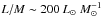 , confirming that this molecule is sensitive to the warm-up. However, of the 23 detected sources, the vast majority have temperatures in the range 30–45 K, and the statistics are poor for high L/M ratios, where the change in temperature is evident. The evolutionary trend must therefore be confirmed with a larger sample and a more extensive set of molecules and transitions, probing a larger range in temperature.
In this work we compare the physical properties derived with commonly-used temperature tracers for a statistically significant sample of high-mass star-forming regions to test the statistical validity of the evolutionary sequence defined by the IR and radio-continuum properties of the source and by L/M, identify the physical process (compression, collapse, accretion, disruption) dominating each phase, and determine the best tracers and transitions to follow the warm-up process, and characterise the emitting region of different species.
2. The sample
The inner ± 60° of the Galactic plane hosts most of the massive stars and clusters in our Galaxy as well as most of its molecular gas (Urquhart et al. 2014b). The APEX Telescope Large Area Survey of the Galaxy (ATLASGAL; Schuller et al. 2009) is the first complete survey at 870 μm of the inner Galactic plane, covering 420 square degrees in the region − 80° ≤ l ≤ −60°, between − 2° ≤ b ≤ 1° and | l | ≤ 60° with | b | ≤ 1.5°. ATLASGAL delivered the most comprehensive inventory of objects at 870 μm within this region at an unprecedented sensitivity (50–70 mJy beam-1) and angular resolution (~ 19.2′′); the survey is complete at 99% above 0.3–0.4 Jy beam-1, allowing to detect all cold and massive clumps with M ≳ 1000 M⊙ within 20 kpc (Contreras et al. 2013; Csengeri et al. 2014; Urquhart et al. 2014a), and thus providing a full census of high-mass star-forming regions in the inner Galaxy.
Taking advantage of the unbiased nature of this survey we selected a flux limited sample, the TOP100 (Giannetti et al. 2014), with additional infrared criteria to avoid biasing the sample towards the hottest and most luminous sources. This sample includes 110 sources and consists almost entirely of clumps that have the potential of forming massive stars, following the criteria of Kauffmann & Pillai (2010) and Urquhart et al. (2013a) (Giannetti et al. 2014; König et al. 2017). The classification for the TOP100 was recently refined in the work by König et al. (2017), separating the sources into four categories, depending on their IR and radio-continuum properties as follows:
-
Seventy-micron weak sources (70w; 16 objects) – sources thatare not detected at 24 μm and show no clear compact 70 μm emission or are seen in absorption at this wavelength, that should represent the earliest stages of the high-mass star-formation process;
-
Infrared-weak clumps (IRw; 33 objects) – clumps associated with a compact 70 μm object, that are not detected in emission in MIPSGAL (Carey et al. 2009) at 24 μm or that are associated with a weak IR source, with a flux below 2.6 Jy corresponding to a B3 star at 4 kpc (Heyer et al. 2016);
-
Infrared-bright objects (IRb; 36 objects) – objects associated with a strong IR source, with a 24 μm flux above 2.6 Jy. If the source is saturated in MIPSGAL we use MSX (Price et al. 2001) to determine the source flux;
-
Compact Hii regions (Hii; 25 objects) – IR-bright clumps also showing radio-continuum emission at ~ 5 or 9 GHz in the CORNISH- (Hoare et al. 2012; Purcell et al. 2013), the RMS surveys (Urquhart et al. 2008, 2009), or targeted observations towards methanol masers (Walsh et al. 1998).
The association radius used for the submm, IR, and radio-continuum sources is 10″, corresponding to the ATLASGAL HWHM and in agreement with the angular separation between high-mass star-formation indicators (e.g. Urquhart et al. 2013a,b). Within each subsample, the sources are among the brightest ATLASGAL clumps in their class. Comparing the distance and mass distributions of the different evolutionary classes, we find that no bias is present for these two parameters; furthermore, the TOP100 includes sources with widely different properties in terms of infrared- and radio-continuum emission, spanning four orders of magnitude in L/M (König et al. 2017). These characteristics make the TOP100 a statistically significant and representative sample of high-mass clumps in the inner Galaxy, and an ideal sample for our purpose to test the evolutionary schemes described in Sect. 1.
The present paper is part of a series investigating the process of high-mass star formation in a broad context. In addition to the work by König et al. (2017), which addresses the dust continuum emission and the total luminosity of the clumps, obtaining the new classification and confirming that the vast majority of the clumps in the sample have the ability to form high-mass stars, we use spectroscopic follow-up observations to characterise the properties of the molecular- and ionised gas. In Giannetti et al. (2014) we study the CO content of the clumps in the TOP100, showing that the abundance of CO is lower than expected in the cold and dense gas typical of clumps in early stages of evolution, and increases to canonical values in more evolved sources, closely mimicking the behaviours of low-mass cores. The TOP100 sample is included in the work of Kim et al. (2017) as well, where mm-recombination lines are used to characterise the ionised gas and identify potentially young compact Hii regions. Mid-J CO lines, observed with CHAMP+ at APEX in a region of 1′ × 1′ around the clumps of the TOP100, are analysed in Navarete et al. (2017) comparing their emission to warm dust, looking for evolutionary trends, and investigating how those commonly found in the low-mass regime change when considering high-mass clumps. Finally, the 36 sources in the first quadrant were studied by Csengeri et al. (2016), focussing on the emission from the outflow tracer SiO and its excitation.
Summary of the observations.
3. Selection of the tracers
To reveal the progressive warm-up of the gas, we needed to rely on efficient thermometers. The selected species should be sensitive to a broad range of physical conditions (i.e. a large number of lines with widely different excitations must be observed), should be abundant, and should have different chemical properties. The latter strongly influences the emitting region of a species, substantially affecting the measured temperature. Using multiple tracers is therefore fundamental to understand the importance of feedback, to characterise the volume of gas that different species probe, and identify those more sensitive to the warm-up process, that is, those with the highest potential for the definition of an evolutionary sequence.
We selected three species, methyl acetylene (CH3CCH), acetonitrile (CH3CN) and methanol (CH3OH). The first two are symmetric top molecules, among the most efficient thermometers available. For each total angular momentum quantum number, J, they have groups of rotational transitions with different K quantum numbers that span a wide range in energy above the ground state, but are close together in frequency. Because K describes the projection of the angular momentum along the symmetry axis, the lowest energy state for each K-ladder is the one with J = K, and the energy of the level increases with increasing K. The group of transitions with J → J−1,ΔK = 0 have increasing energy for higher values of K (see e.g. Kuiper et al. 1984). The dipole moment for these species is parallel to the symmetry axis, therefore radiative transitions with ΔK ≠ 0 are forbidden: different K-ladders are connected only through collisions, and this makes their ratio sensitive to the kinetic temperature (Bergin et al. 1994). The relative intensity of J → J−1 groups between different J levels, on the other hand, can potentially depend on density, too. The great potential of these molecules resides, therefore, in the separation of temperature and density effects in their excitation.
Methyl acetylene has a small dipole moment of 0.7804 D (Muenter & Laurie 1980). Several works have shown that the lower J lines of this molecule are thermalised for densities of molecular hydrogen ~ 104 cm-3 (Askne et al. 1984; Bergin et al. 1994). Because of these properties, CH3CCH is commonly used as a thermometer: it is found to have an extended emitting region and to trace relatively cold gas (e.g. Fontani et al. 2002; Bisschop et al. 2007).
CH3CN has a larger dipole moment (3.922 D, Gadhi et al. 1995), and is therefore harder to thermalise. Several works discuss the use of this molecule as a temperature tracer in astrophysical environments (e.g. Askne et al. 1984; Bergin et al. 1994). Acetonitrile is the prototypical hot core tracer; indeed it is classified solely as a “hot” species by Bisschop et al. (2007) and it is one of the first choices to derive the gas properties in the hot gas therein (e.g. Remijan et al. 2004; Sanna et al. 2014). Chemical models of star-forming regions, however, predict two abundance peaks for this molecule (Garrod et al. 2008): the early-time peak follows the evaporation of HCN from grains, from which CH3CN is formed in the gas phase through  (1)the late-time peak, on the other hand, is due to direct evaporation of acetonitrile from the dust grains for temperatures in excess of ~ 80–100 K, leading to abundances ~ 2 orders of magnitude higher than in the cold gas, explaining the efficacy of this species in tracing hot material.
Methanol is widespread in the ISM and it is one of the basic blocks for the formation of more complex, biologically relevant molecules (e.g. Garrod & Widicus Weaver 2013). CH3OH is a slightly-asymmetric rotor, that can be effectively used as a probe of temperature and density in interstellar clouds (Leurini et al. 2004, 2007b). This species is formed through surface chemistry by successive hydrogenation of CO, and it is found to be one of the major constituents of ice mantles on dust grains (Gibb et al. 2004). Its strong binding energy to the grain surface, due to hydrogen bonding, determine the co-evaporation of CH3OH with water at ~ 110 K and a strong enhancement of the abundance in hot cores. The abundance in hot gas is consistent with that observed in ices in cold protostellar envelopes, indicating that the molecules there are directly sublimated from the mantles (Garrod & Widicus Weaver 2013). Methanol is found in cold gas as well (Smith et al. 2004), which poses a long-standing problem in understanding how this species is released into the gas phase at such low temperatures. Proposed mechanisms include, for example, spot heating, shocks, and exothermic reactions on the grain surface (e.g. Roberts et al. 2007, and references therein).
In the following we shall compare the physical properties traced by these species to search for evidence of progressive warm-up in the evolutionary sequence defined by the infrared and radio-continuum properties of the clump and its L/M ratio. In addition we will characterise the volume of gas that these molecules are tracing, and we will compare the results with other tracers from previous works on the same sample: submm dust emission by König et al. (2017), NH3 (1, 1) and (2, 2) inversion transitions from Wienen et al. (2012), and CO isotopologues from Giannetti et al. (2014).
4. Observations
We observed multiple lines of CH3CN, CH3CCH, and CH3OH, with the APEX, IRAM-30 m, and Mopra telescopes, between 85 GHz and 350 GHz. Table 1 gives an overview of these observations. All line temperatures in this work are reported in the main-beam temperature scale, according to the efficiencies listed in the table.
4.1. IRAM-30 m
Thirty-six of the TOP100 sources are observable from the northern sky and were observed in the 3-mm band with the IRAM-30 m telescope. These observations were previously presented by Csengeri et al. (2016) and we refer the reader to their paper for a detailed discussion. The authors report a calibration uncertainty ≲ 10%. These observations were carried out between the 8th and 11th of April 2011. The velocity resolution of the lines reported in this paper is listed in Table 1.
4.2. Mopra
The observations were carried out with the ATNF Mopra 22 m telescope in May 2008 as pointed observations in position switching mode. The HEMT receiver was tuned to 89.3 GHz and the MOPS spectrometer was used in broadband mode to cover the frequency range from 85.2–93.4 GHz with ~ 0.9 km s-1 velocity resolution. The beam size at these frequencies is ~ 35″. The typical observing time per source was 15 min. The system temperature was 200 K on average. Pointing was checked every hour with line pointings on SiO masers. Each day G327 and M17 were observed as a check in the line setup chosen for the survey. The calibration uncertainty for this dataset is 20%.
The processing of the spectra resulting from the on-off observing mode, the time and polarisation averaging, and baseline subtraction were done with the ASAP package. The data was then exported to the CLASS spectral line analysis software of the GILDAS package for further processing.
4.3. APEX
The FLASH+ (Klein et al. 2014) heterodyne receiver on the APEX 12 m telescope was used to observe the ATLASGAL TOP100 sample in CH3CN (19–18), CH3CCH (20–19), and CH3OH (7–6) on June 15th and 24th, August 11th, 23rd, 24th and 26th 2011. The observations were performed in position switching mode with reference positions offset from the central position of the sources by (600′′, 0′′). Pointing and focus were checked on planets at the beginning of each observing session. The pointing was also regularly checked on Saturn and on hot cores (G10.62, G34.26, G327.3−0.6, NGC 6334I and Sgr B2 (N)) during the observations. Comparison of sources observed multiple times show that the calibration uncertainty is ≲ 15% for this dataset.
5. MCWeeds
To extract physical parameters from this large set of lines, a simultaneous fit was performed, including all available spectra for a given source. Weeds (Maret et al. 2011) provides a simple and fast way to generate synthetic spectra assuming LTE, but lacks automatic optimisation algorithms. Here PyMC (Patil et al. 2010) comes into play, implementing Bayesian statistical models and fitting algorithms; therefore we developed MCWeeds, providing an external interface between these two packages to automatise the fitting procedure.
MCWeeds allows to simultaneously fit the lines from an arbitrary number of species and components, combining multiple spectral ranges. The fitting is performed using one of the methods offered by PyMC, that is, maximum a posteriori estimates (MAP), “normal approximations” (NormApprox; Gelman et al. 2003) or Monte Carlo Markov chains (MCMCs)1. This is therefore a very flexible approach, giving the possibility of obtaining both a very fast fitting procedure or a very detailed one, generating probability distribution functions for each of the model parameters. MCWeeds can be accessed both from inside CLASS or from shell.
A simple flow chart of the main steps performed by the programme is shown in Fig. 1. As indicated in the figure, an input file must be defined, containing all the information to perform the fit, including: the species that must be included in the fit, the spectral ranges to be considered and the corresponding data file, the fitting algorithm to be used and its parameters, and the priors or the values for all of the models parameters (i.e. column density, temperature, size of the emitting region, radial velocity and linewidth for each species, rms noise, and calibration uncertainty for each of the spectral ranges). MCWeeds retrieves the spectra in the specified frequency ranges from the data files, and the line properties from the JPL- (Pickett et al. 1998), CDMS- (Müller et al. 2001), or a local database, to generate the synthetic spectrum, given the model parameters. The PyMC model is automatically built using the priors specified in the input file; the likelihood is computed as the product of the probabilities for each channel, assuming a Gaussian uncertainty, with a σ equal to the rms noise.
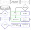 |
Fig. 1 Simple schematic flow-chart of MCWeeds. The steps performed when using MCMCs are highlighted in blue and those for MAP or normal approximation in green. A more detailed description is given in the text. |
A detailed discussion of priors, their meaning and choice can be found in, for example, Jaynes & Bretthorst (2003). For the purposes of the present work, the definition of a prior for the fit parameters avoids the generation of unphysical parameters (e.g. a negative linewidth, or temperature) during the fit procedure, as well as giving the possibility to incorporate any previous information available in the fit (see Sect. 5).
The fit is performed according to the method specified in the input file, as indicated in the first decision box of Fig. 1. In the case of MAP or NormApprox, the optimisation is performed with one of the methods available in SciPy optimize package. For MCMCs a set of parameters is generated, which is used to derive the synthetic spectrum. The model spectrum is compared to the observations; the likelihood P(D | M) (the probability of the data given the model) and the posterior P(M | D) (the probability of the model given the data) are computed. Based on this, the newly-generated set of parameters is accepted or rejected (see, e.g. Hastings 1970), and the procedure is repeated until the number of iterations requested is reached (last decision point). Finally, the results are summarised in an HTML page, containing the best fit parameters, their uncertainties, the best fit spectrum superimposed on the observations and, for MCMCs, the probability distribution function, the trace plot and the autocorrelation of each of the fit parameters. When using MCMCs additional convergence tests can be performed:
-
the Raftery-Lewis procedure (Raftery &Lewis 1995) estimates the number of iterationsrequested to achieve convergence, as well as the burn-in periodand the thinning factor (see Sect. 5) to getindependent samples;
-
the Geweke test (Geweke 1992a), that checks whether the mean estimates converged by comparing the mean and the variance of the samples in consecutive intervals from the beginning and the end of the chains;
-
and the Gelman-Rubin statistic (Geweke 1992b), which tests if multiple chains converge to the same distribution from random starting points, comparing the variance within- and between chains.
Example of the fits produced with MCWeeds in the context of this work are shown in Figs. 2–4, for CH3CCH, CH3CN, and CH3OH, respectively. Trace plots, probability distribution functions, and autocorrelation plots are shown in Figs. A and A.1 in the online material.
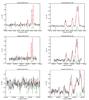 |
Fig. 2 Example of the fit performed with MCWeeds for CH3CCH. The K components are indicated in green. The best fit model is shown in red. The source on the left is an IRw and the source on the right belong to Hii. |
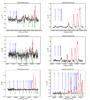 |
Fig. 3 Example of the fit performed with MCWeeds for CH3CN. The K components of CH3CN are indicated in green and those of CH313CN are indicated in blue. The best fit model is shown in red. The source on the left is an IRw and the source on the right belong to Hii. |
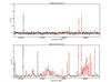 |
Fig. 4 Example of the fit performed with MCWeeds for CH3OH. The best fit model is shown in red. The lines not reproduced by the model are contaminating species and are excluded from the spectral ranges used for the fit (cf. Table 2) The top panel show the results for an IRw source and the bottom panel for an Hii. The νt = 1 band is visible between ~ 337 500 and ~380 000 MHz. |
The synthetic spectrum is produced according to the following equations (Comito et al. 2005; Maret et al. 2011): 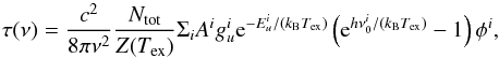 (2)
(2)![\begin{equation} \tb(\nu) = \eta \left[ J_\nu(\tex) - J_\nu(\tbg) \right] \left( 1 - \expo{-\tau(\nu)} \right)\label{eq:weeds_tb}, \end{equation}](/articles/aa/full_html/2017/07/aa30048-16/aa30048-16-eq76.png) (3)where τ(ν) and TB(ν) are the line optical depth and brightness temperature at a given frequency ν; kB is the Boltzmann constant, h is the Planck constant, Ntot is the column density of the molecule considered, Z(Tex) is the rotational partition function, Ai is the Einstein coefficient for spontaneous emission,
(3)where τ(ν) and TB(ν) are the line optical depth and brightness temperature at a given frequency ν; kB is the Boltzmann constant, h is the Planck constant, Ntot is the column density of the molecule considered, Z(Tex) is the rotational partition function, Ai is the Einstein coefficient for spontaneous emission,  ,
,  ,
,  are the upper level degeneracy and energy, and the rest frequency of line i, and φi is its profile. Tex and TBG are the excitation temperature and the background temperature, respectively. We assumed that the lines have a Gaussian profile and that TBG = 2.73 K. In Eq. (3), η is the beam dilution factor, calculated as:
  (4)where ϑs and ϑbeam are the source- and beam FWHM sizes.
Wilner et al. (1995), on the basis of the calculations by Rowan-Robinson (1980) and Wolfire & Cassinelli (1986), show that the temperature structure in a clump heated by a central massive star can be described by the power-law: ![\begin{equation} T = 233 \left(\frac{L}{\lsuntab} \right)^{\frac{1}{4}} \left(\frac{R}{\mathrm{AU}} \right)^{-\frac{2}{5}} \rm [K],\label{eq:t_str} \end{equation}](/articles/aa/full_html/2017/07/aa30048-16/aa30048-16-eq97.png) (5)where R is the radius of the region with a temperature T, around a star with bolometric luminosity L. We therefore inverted this expression to define the size of the emitting region as a deterministic variable, dependent on the bolometric luminosity of the source, and on the temperature generated in each step of the chain (see below). Assigning a size for the emitting region of each species and component allows us to derive η, correcting for the dilution; this correction considers the appropriate beam for each combination of frequency and telescope.
(5)where R is the radius of the region with a temperature T, around a star with bolometric luminosity L. We therefore inverted this expression to define the size of the emitting region as a deterministic variable, dependent on the bolometric luminosity of the source, and on the temperature generated in each step of the chain (see below). Assigning a size for the emitting region of each species and component allows us to derive η, correcting for the dilution; this correction considers the appropriate beam for each combination of frequency and telescope.
With respect to conventional rotation diagrams, our method has several advantages: firstly, the opacity is taken into account for each line, secondly, all lines have the same intrinsic width, because line broadening by optical depth effects is taken into account, and lastly, blending of the lines can be taken into account including the contaminating species in the routine.
The spectral ranges used and the priors considered in the model for each molecule of interest are listed in Tables 2 and 3, respectively. We used loosely-informative priors for the parameters of the fit, choosing broad Gaussian functions centred on representative of typical values of temperatures, column densities and linewidths in regions of high-mass star formation (e.g. van der Tak et al. 2000; Fontani et al. 2002; Beuther et al. 2002). For the source radial velocity we chose a mean (μ) equal to the measured velocity in C17O(3–2) from Giannetti et al. (2014) (if C17O J = 3 → 2 was not detected, we use the velocity of N2H+J = 1 → 0 from the 3 mm surveys; see Urquhart et al., in prep., and Csengeri et al. 2016). For the linewidths and the temperatures we used truncated Gaussians (the lower and upper limits are indicated in Table 3 with “low” and “high”, respectively), in order to exclude very low, highly unlikely values for the analysed data; the upper limits are sufficiently high to have no impact on the procedure. For the hot component we increased the mean of the priors, in agreement with the idea that the material in the hot core is warmer and more turbulent; we also scaled the mean of the column density distribution using Eq. (4), assuming a size of ~ 1″. As a final remark, in the case of temperature, we made use of the prior to keep the cool and the hot components distinct, by defining non-overlapping domains, separated at 100 K. Multiple priors were tested, to ensure that the results are not significantly influenced by this choice; the fit has very strong observational constraints that dominate the information. Values of the rotational partition functions used, evaluated for a set of temperatures, are listed in Table 4. The values of the partition function Z for the temperatures in our modelling were determined by interpolation, using a linear fit of the measured values in a log (T) vs. log (Z) space.
In order to obtain the full posterior distribution, and thus the most accurate estimates for the parameters, as well as their uncertainties, the spectra were fitted using MCMCs with an adaptive Metropolis-Hastings sampler as the fitting algorithm (Haario et al. 2001). The number of iterations for CH3CCH and CH3OH was set to 210 000 for each source, the burn-in (number of iterations to be discarded at the beginning of the chain, when the distribution is not yet representative of the stationary one; Raftery & Lewis 1995) was chosen to be 50 000, and the thinning factor (number of iterations to be discarded between one sampling and the next, to minimise correlation between successive points; Raftery & Lewis 1995) was set to 20 for CH3CCH and to 50 for CH3OH. The adaptive sampling was delayed by 20 000 iterations (i.e. the number of iterations performed before starting to tune the standard deviation of the proposal distribution; Haario et al. 2001). For CH3CN we used longer chains with 260 000 iterations, a burn-in of 60 000 and a delay of 30 000; we used a thinning factor of 50 for this species as well. For each molecule and iteration, a set of column density, velocity, linewidth and temperature was generated. According to Eq. (5), from the generated temperature and bolometric luminosity of the source (taken from König et al. 2017), a size of the emitting region was computed and translated to arcseconds using the distances listed in Table A.1. For isotopologues, all parameters were the same, except for column density, which was reduced by a factor equal to the relative isotopic abundance. In order to take into account the uncertainty in the relative calibration of different telescopes and wavelengths, we used different calibration factors for the separate J multiplets of CH3CCH and CH3CN. This allowed the programme to rescale the spectra by a normally-distributed factor with mean one and σ = 0.07, according to Sect. 4; this distribution was truncated at a maximum of 30% in either direction.
Spectral ranges used for the fit.
Priors used in the models for the molecules of interest.
Measurements of the rotational partition function for the species of interest.
In order to account for contamination and for strong lines in the spectra, CH3OCHO, C2H5CN, 33SO2, and c-C3H were included in the model of methyl acetylene (these lines are relevant only for the J = 20 → 19 multiplet in bright sources, like the one shown in Fig. 2, right); CCH, CH3OCHO, and CH3OH are considered for that of acetonitrile. All methyl acetylene lines, from (5–4) to (20–19), are well described by a single temperature component; on the other hand, CH3CN and CH3OH need a second temperature component for sources detected in the highest excitation lines, as discussed in Sect. 6. The radial velocity of both temperature components is assumed to be the same, whereas all other parameters are independent. To take into account the variation of the 12C/13C isotopic ratio with galactocentric distance, we use the relation ![\begin{equation} \frac{[^{12}\mathrm{C}]}{[^{13}\mathrm{C}]} = 6.1 D_{\rm GC} [\mathrm{kpc}] + 14.3\label{eq:c_isotopic_ratio} \end{equation}](/articles/aa/full_html/2017/07/aa30048-16/aa30048-16-eq146.png) (6)from Giannetti et al. (2014), and we fix the carbon isotopic abundance for each source to the appropriate value obtained with this expression.
(6)from Giannetti et al. (2014), and we fix the carbon isotopic abundance for each source to the appropriate value obtained with this expression.
6. Detection rates and fit results
In the following we consider only sources with a “good detection”, that is, those sources detected with a S/N> 3 for at least two transitions. Detection rates for individual molecules are listed in Table 5, and the number of observed sources per species is indicated. The table also shows how the detection rate depends on the evolutionary class for the TOP100, increasing with time, from 30–40% for sources quiescent at 70 microns, up to 95–100% for Hii regions. In addition, for the analysis we discard all the sources with a 95% highest probability density (HPD) interval exceeding 20 K for cool components and 60 K for hot components. This removes sources with excessive uncertainties in the temperatures. Tests with model spectra show that in these cases the best-fit temperature is overestimated.
Detection rates for the different species considered in this work.
Properties obtained with the different species considered in this work.
The extensive set of observations that we have for the TOP100 now permits us a consistent comparison of properties of the gas as traced by different molecules. Examples of the fit obtained with MCWeeds for CH3CCH, CH3CN, and CH3OH are shown in Figs. 2–4, respectively. The complete results of the fitting procedure are reported in Tables A.2 to A.8; figures are incorporated in the ATLASGAL database, and can be accessed at atlasgal.mpifr-bonn.mpg.de/top100. In addition to the fit images, the trace of the chain, the distributions of the values, and the autocorrelation plots are available for each of the parameters of interest. Figures A and A.1 show examples of these plots for two sources in the TOP100.
In Giannetti et al. (2014) several sources in the TOP100 show multiple velocity components along the line-of-sight in low-J transitions of CO isotopologues. Because of the line series of the methyl acetylene and acetonitrile, and the close-by trasitions in the methanol band, multiple velocity components may complicate the derivation of temperatures and column densities. In contrast to what is found with CO isotopologues, the species considered in this work have relatively simple spectra, characterised by a single velocity component. The only source clearly showing two components is AGAL043.166+00.011, which was excluded from the following analysis. The difference in velocity among different tracers is within 1 km s-1, in line with the spectral resolution of the data. This, in combination with the fact that only a single velocity component is observed for the more complex species considered in this work, makes it easy to identify the main contributor to the dust continuum emission observed in ATLASGAL and HiGAL (Molinari et al. 2010) and analysed in König et al. (2017).
Temperatures obtained from the data of different species can be systematically different, but they are always correlated, as discussed in more detail in Sect. 7. The properties of the emitting material for the different tracers are summarised in Table 6 and illustrated in Fig. 5, which shows the empirical cumulative distribution function (ECDF, built with all good detections, using the best-fit results) of: a) temperature; b) line FWHM; c) size of the emitting region and d) column density for all available species. In addition, thanks to the association of a spatial scale for the emitting region of different species and temperature components, we could correct for the beam filling factor, deriving source-averaged abundances relative to H2 (see Fig. 6 and Table 6). Opacity effects were also accounted for directly in the models (cf. Eqs. (2) and (3)), and by simultaneously fitting the 13C-substituted isotopologue of acetonitrile. In deriving the abundances we considered two cases, comparing the size of the emitting region (ϑs), as obtained from the fit, with the beam size (ϑb): ϑb ≳ ϑs and ϑb ≪ ϑs. In the former case, we computed the abundance as the ratio:  (7)where
  and
and  . Here M(r<R) indicates the mass within a radius R derived from the fit, obtained by scaling the total mass from the SED fit assuming that nH2 ∝ r-1.5, consistent with the measurements by Beuther et al. (2002). Assuming a different value for the power-law slope has an impact on the measured abundances; the effect of varying the exponent between − 1 and − 2 is discussed in the next sections. On the other hand, if the beam size is much smaller than the size of the emitting region, we derive the abundance in the usual way, as the ratio of column densities:
  (8)the column density of molecular hydrogen is taken from König et al. (2017). Below we briefly summarise the fit results for each molecule.
6.1. Methyl acetylene
The simultaneous fit of the (5–4), (6–5) and (20–19) series indicates that CH3CCH emission can be satisfactorily reproduced with a single temperature component. Figure 5 shows that the temperatures derived using methyl acetylene range between 20 K and 60 K, associated with narrow linewidths, consistent with those observed for C17O(3–2). The fit shows that the emitting region for CH3CCH is of the order of 0.5 pc (Fig. 5), or 25″ at 4 kpc. Together with the necessity of a single temperature component to fit lines with a wide range of excitations and the non-detection of high-excitation lines, this indicates that this species is tracing the bulk of the dense gas in the clump, and it is not significantly enhanced at high temperatures.
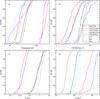 |
Fig. 5 Empirical cumulative distribution functions for a) temperatures, b) line FWHMs, c) source diameter, and d) molecular column density. The different tracers and components are drawn with different colours, as indicated in the legend in the lower right corner of panel b). “CO” refers to properties obtained from C17O and C18O transitions from Giannetti et al. (2014), and NH3 properties are taken from Wienen et al. (2012). Dust properties from König et al. (2017) are included only in panels a) and c). |
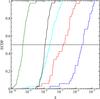 |
Fig. 6 Empirical cumulative distribution function for the abundance relative to molecular hydrogen. CH3CCH, and the hot and cool components of CH3CN and CH3OH are drawn with different colours, as indicated in panel b) of Fig. 5. |
The minor systematic adjustments to the calibration factors (see Sect. 5) of the spectra for different J transitions lends support to the claim that this molecule is not too far from LTE, as discussed in Bergin et al. (1994). In fact, if it were subthermally excited, high-J transitions would be systematically fainter. The column densities of CH3CCH are found to be in the range 2.3 × 10¹⁴−3.6 × 1015 cm-2 (central 90% credible interval, hereafter CI; all ranges refer to this interval), corresponding to abundances with respect to H2 between 5 × 10⁻⁹ and 2.8 × 10⁻⁸ (Fig. 6 and Table 6), calculated with Eq. (7). Varying the power-law index for the density profile by ±0.5 changes the abundance by approximately ~20–30% up or down, depending on the value of the exponent. Linewidths are narrow, distributed between 1.9–6.4 km s-1 (Fig. 5), with a median of ~3.5 km s-1.
6.2. Acetonitrile
Combining the (5–4) and (6–5) transitions with the (19–18), we find that two temperature components are necessary to reproduce all observed lines for the 34 sources detected in the line series observed as part of the FLASH+ survey. On the one hand, warm gas dominates at 3 mm, with temperatures virtually always in the range ~ 30–80 K (hereafter the cool component), and column densities between 1.0 × 10¹³−2.6 × 1014 cm-2. This component also contributes significantly to the K = 0,1 of the (19–18), but it is not sufficient to excite the higher-K lines. The linewidths characterising acetonitrile are broader than those of C17O and methyl acetylene, with a median of ~ 5.4 km s-1 (3.9–8.9 km s-190% CI), showing that the material traced is more turbulent. The emitting region of this component is of the order of ~ 0.4 pc, or ~ 20″ at 4 kpc. According to Eq. (7) the median abundance of CH3CN in the warm gas is ~ 4.6 × 10⁻¹⁰. The variation of the density profile imply variations of a factor 1.5 for the abundance. When properly accounting for opacity effects and contamination by hot material, we find that acetonitrile is not exclusively a hot core tracer, but is abundant also at lower temperature, extending over dense regions in the clump. On the other hand, hot gas is responsible for the emission in high-excitation lines. To adequately reproduce the (19–18) multiplet, temperatures of ~ 200 K are needed (Fig. 3, right); the emitting region is of the order of 0.01 pc, broadly in line with typical properties of hot cores (e.g. Cesaroni 2005; Sanna et al. 2014). The very small emitting region implies very high column densities, with a median value of ~ 1017 cm-2 (due to the small filling factor), which translates to a median abundance of 1.6 ~ 10-7. If the power-law index for the density profile changes by ± 0.5, the abundance is scaled by approximately a factor of ~ 10 in each direction. The lines are sligthly broader than for the cool component, with a median of ~ 6.6 km s-1.
6.3. Methanol
The FLASH+ survey covers the Jk (7–6) band, both from the torsional ground state (νt = 0) and the first torsionally-excited state (νt = 1). The significant difference in excitation of the lines in the two torsionally excited states makes our observations sensitive to both hot and cold gas; in fact, a temperature in excess of 150 K is needed to reproduce the lines of the first torsionally-excited state for the band at 337 GHz.
Methanol is the species with the highest absolute detection rate, with only a very weak dependence on the evolutionary class (see Table 5). A total of 35 sources are detected also in the νt = 1 state, which mainly belong to the most evolved clumps. Similarly to CH3CN, in these sources the full set of lines is well reproduced only when including a second, hot component in the fit. CH3OH traces the lowest temperatures among all the considered tracers, between 10–30 K. Methanol is, as mentioned in Sect. 3, a slightly-asymmetric rotor and the line ratios for this species are sensitive to both temperature and density (Leurini et al. 2004, 2007b). Therefore, the excitation temperature measured under the assumption of LTE may not be representative of the emitting gas kinetic temperature, and consitutes a lower limit for this quantity. Leurini et al. (2007b) perform non-LTE modelling of this molecule in a sample of high-mass star-forming regions, showing that kinetic temperatures of the emitting gas range between 17 and 36 K; the effect of non-thermalisation on the measured temperature is therefore non-negligible, but likely small. A direct comparison between LVG and LTE modelling for the same source is carried out by Leurini et al. (2004), finding similar column densities, but a lower temperature (10 vs. 17 K) assuming LTE. In our model of a spherical clump with a power-law gradient in temperature, the emitting region is always more extended than the beam for the cool component. The column densities are found to range between 4.0 × 1014 cm-2 and 1.1 × 1016 cm-2, which are translated to a median abundance of ~ 2.3 × 10⁻⁸ (Fig. 6), again demonstrating that methanol is very abundant also in cold gas. The temperatures traced by torsionally-excited lines on the other hand, are only marginally lower than those determined with acetonitrile, with a median of ~ 180 K, coming from a region a few hundredths of a parsec in size. The properties of the gas traced by these transitions are in good agreement with interferometric studies (e.g. Leurini et al. 2007a; Beuther et al. 2007). CH3OH, as expected, is more abundant in hot gas on average by a factor ~ 100, due to the evaporation from grains (Fig. 6). If the density power-law exponent is changed between − 1 and − 2, the abundance in the hot gas is modified by a factor ~ 5 up and down. The linewidths of methanol transitions are consistent with those of CH3CN in cold gas, although the temperatures derived are closer to C17O, and marginally larger in hot gas.
Median temperature per class, as measured with all molecular tracers considered.
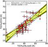 |
Fig. 7 Correlation between the temperature as measured by CH3CN and CH3CCH. All the other combinations between the tracers analysed are included in the online material in Fig. A. The best fit is shown as a blue solid line. The uncertainties due to the line parameters are indicated by the shaded region – dark- and light yellow for 68% and 95% HPD intervals, respectively. The intrinsic scatter in the relation is indicated by the dashed black lines. At the bottom right of the panels the Spearman correlation coefficient is indicated. |
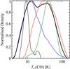 |
Fig. 8 Kernel density estimate of the probability density function, normalised to its maximum for displaying purposes, for the excitation temperature as traced by CO isotopologues. The thin lines represent the different classes: black – 70w, blue – IRw, red – IRb, and green – Hii. The thick black line refer to the entire TOP100 sample. |
7. Discussion
In Sect. 6 we found that all temperatures from the different molecules are correlated. Figures 7 and A summarise these results. The tightest correlations are found between methyl acetylene, acetonitrile and dust, which confirms that they are good tracers of temperature in the envelope. C17O is also well correlated with these tracers, but shows a much larger scatter and uncertainties. The dust temperature for the sources in the TOP100 was derived and discussed in detail in König et al. (2017). Comparing their values with those obtained using the other probes available, we find that dust is tracing systematically lower temperatures than CH3CN and CH3CCH; this can be explained as a combination of the different regions over which the emission is integrated (only the dense, central region around the dust emission peak for molecular lines and the entire clump for dust), and the fit of the warm gas emission in the SED with a second component (see König et al. 2017). That a higher temperature is derived from CH3CN compared to CH3CCH indicates that the abundance of the former tracer is markedly more sensitive to the star-formation activity, which is also supported by the larger measured linewidths. The methanol results show weaker trends with respect to CH3CN and CH3CCH, suggesting that it is not as good as these species as a tracer of warm-up. It is characterised by a marginal change in the measured temperature along the evolutionary sequence for the cool component (cf. Table 7). On the other hand, the temperature of the hot component is well correlated with that measured with CH3CN. Ammonia does not stand out as an optimal tracer for warm-up when using only the low-excitation JK = (1,1) and (2,2) radio inversion lines, despite being commonly used as a thermometer. The median temperature traced by NH3 varies of only a few degrees Kelvin along the entire evolutionary sequence, as observed in previous works (e.g. Wienen et al. 2012; Giannetti et al. 2013, and Table 7). This molecule has the lowest correlation coefficients with the other tracers, in part because it was observed with a much larger beam (see Wienen et al. 2012). The temperature from NH3 best correlates with Td, which is consistent with the ammonia tracing an extended region (see also Sect. 7.4), similar to that used to compute the SEDs. However, in a Td vs.TNH3 the best-fit relation shows that, with respect to dust, NH3 traces hotter material in very cold sources and colder gas in warmer, more evolved clumps, reducing the differences between different classes.
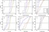 |
Fig. 9 Comparison between empirical cumulative distribution functions of the temperature for the four evolutionary classes defined for the TOP100. Each panel show one of the species analised in this work. The four evolutionary classes are indicated in a different colour, according to the legend shown in the lower right corner of panel c). The solid line at p = 0.5 shows the median of the distributions. |
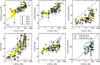 |
Fig. 10 L/M ratio vs. temperature. The black solid line indicates the line-of-sight- and beam-averaged temperature for a spherical clump model passively heated by a central object accounting for the total luminosity. The thick grey line shows the non-parametric regression of the data, with uncertainties indicated by the yellow-shaded area. |
7.1. Temperature distribution from CO isotopologues: separation between IR-weak and IR-bright sources
The four evolutionary classes defined for the TOP100 by König et al. (2017), and used throughout this work, separate IR-bright and IR-weak sources on the basis of their 24 μm fluxes, using a threshold of 2.6 Jy, which roughly divides sources that need a hot component to fit the complete SED from those that do not.
A kernel density estimation (Rosenblatt 1956; Parzen 1962) for the CO isotopologues excitation temperatures from Giannetti et al. (2014) shows a minimum at ~ 20 K (Fig. 8), corresponding to the CO evaporation temperature, confirming that, once CO is evaporated back into the gas phase, the gas traced is hotter, and more closely affected by the feedback from young stellar objects. The CO temperature also nicely separates IRw and IRb: these two classes are thus not only different in terms of temperature, but also represent objects in which CO is mostly locked onto dust grains in dense gas for the former class, and in which it is mostly in the gas phase for the latter. This gives a clear physical meaning to the threshold chosen by König et al. (2017) to distinguish these two classes. Therefore, the four classes defined for the TOP100 all represent physically distinct evolutionary stages.
7.2. Feedback from high-mass YSOs: warm-up of the gas
The feedback from forming stars causes the progressive heating of the surrounding gas. Thanks to the fact that the TOP100 is a representative sample of high-mass star-forming regions in different evolutionary stages we can evaluate this effect by comparing all the available tracers for the different groups of objects, to validate the scheme used to classify them. To test whether we see the gas being heated by the feedback from the nascent massive young stellar objects, and determine to what degree the various species are influenced by it, we divided the TOP100 in the four classes described in Sect. 2, to compare the ECDFs of the temperature for each molecule (Fig. 9). We then made use of the Anderson-Darling test (Scholz & Stephens 1987), implemented in the R package kSamples2, to assess whether or not they are drawn from a common distribution. The tests show that the temperatures found in consecutive classes (70w, IRw, IRb, Hii) increase, with p-values always below 0.9% (cf. Table 8), allowing to reject the null hypothesis that the temperature is not increasing in more evolved sources at a level >2.5σ, for methyl acetylene and acetonitrile, the best thermometers available to us. The typical temperature of each class also appear different and increasing from methanol. This confirms the trends seen in dust temperature (König et al. 2017), ammonia (e.g. Wienen et al. 2012) and CO (Giannetti et al. 2014).
In conclusion, we find that all probes indicate a progressive warm-up of the gas with evolution, albeit with significantly different behaviours which are determined by the properties of the species and of the transitions. Methyl acetylene and acetonitrile are the most sensitive to the warm-up process, methanol and ammonia (when using the two lowest inversion transitions) show only a marginal increase in temperature along the evolutionary sequence.
Whereas the classes defined for the TOP100 on the basis of the IR- and radio continuum properties of the clumps only allow for a comparison between their average properties, the L/M ratio defines a continuous sequence in time. We can thus investigate directly whether the temperature and the L/M ratio are correlated. In Fig. 10 we show the temperature traced by all molecular probes available for the TOP100 as a function of the luminosity-to-mass ratio. A non-parametric regression3 with bootstrapped uncertainties (estimated using the 2.5% and 97.5% quantiles) was performed for each tracer with the R package np (Hayfield & Racine 2008): it indicates that a correlation between these parameters exists for all tracers, confirming that L/M is a good indicator of evolution as well (e.g. Molinari et al. 2008, 2016), and that the forming cluster has a strong impact on the physical properties of the surrounding environment on a clump scale.
A simple toy model was constructed, considering a spherical clump with power-law density and temperature profiles; the line-of-sight and beam-averaged temperature was calculated at the peak of column density, to be compared with the available tracers for the TOP100. The density gradient was assumed to be proportional to r-1.5. Consistently with the analysis performed through MCWeeds, the T-profile is described by Eq. (5). The average temperature was calculated by weighting the values in individual pixels by the mass in that pixel and beam response, assuming it is Gaussian. The results are superimposed to the data points in the panels of Fig. 10.
Resulting p-values of Anderson-Darling tests for the three species considered in this work.
CH3CCH and CH3CN:
Methyl acetylene and acetonitrile are in good agreement with this simple model for L/M ratios above a few  , confirming that these molecules are reliable tracers of physical properties and passive heating in the dense layers of the clump. Changing the slope of the density profile by ± 0.5 moves the curve up or down, enveloping the data points for these two molecules. As discussed in Sect. 3, CH3OH and CH3CN are formed mainly on dust grains and are released in the gas phase for temperatures above 80–100 K. With this in mind, to compare the results of the hot components to the model, we only considered in the average the regions where the temperature exceeds 80 K, in which the abundance is substantially increased. The bottom right panel of Fig. 10 shows the results of this procedure: the trend and average T are well reproduced for acetonitrile.
The good match of the observed T vs.L/M relation for  for CH3CCH, CH3CN, and, to a lesser degree, C17O from Giannetti et al. (2014) with the predictions of our spherical clump model, centrally heated by a star having a luminosity equal to the observed bolometric luminosity, indicates that the heating of the gas in the cluster environment is dominated by its most massive member. This supports the findings by Urquhart et al. (2014c), showing that the observed bolometric luminosity agrees better with the luminosity of the most massive star, rather than the luminosity of the entire cluster, for clumps with M> few × 103M⊙ (adopting the ATLASGAL fluxes from Contreras et al. 2013; the masses obtained with these fluxes are typically a factor of ~ 3 higher than obtained from the SEDs, König, priv. comm.). The authors argue that this lends support to the idea that high-mass stars form first, while the rest of the cluster members must yet reach the ZAMS, thus having a minor contribution to Lbol. A similar conclusion is obtained by Zhang et al. (2015), and Sanna et al. (2014) show that at least in the case of the high-mass star-forming region G023.01–00.41, the luminosity and the feedback are indeed dominated by the most massive star.
Acetonitrile is vastly undetected in cold and young sources with  and this is not simply a column density effect. Assuming that CH3CN has an abundance equal to the median in the detected sources for the cool component, the column density should be sufficient to detect this molecule: the predicted CH3CN column densities are found to range between 1–6 × 1013 cm-2, suggesting a lower abundance or central density, or a smaller emitting region. In contrast to acetonitrile, all other molecules are detected in several sources in the interval
 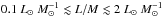 . The temperature derived from methyl acetylene in this interval of L/M is approximately 20 K and relatively constant. Our toy model predicts a temperature lower than observed, possibly suggesting that some mechanism providing additional heating is present. It is interesting to note that, according to Urquhart et al. (2014c), the distribution of sources associated with a massive YSO or an UCHii region in a M−L plot is enveloped by two lines of constant luminosity-to-mass ratios, between
  and
and  . The lower threshold in L/M well matches the flattening of the temperature as a function of L/M for CH3CCH, as well as the detection threshold for CH3CN.
Molinari et al. (2016) find a similar behaviour for the temperature traced by CH3CCH, using the J = 12 → 11 rotational transition, but for sources in the range 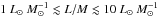 , levelling to ~ 35 K. The authors discuss how this can be caused by the excess heating of the forming cluster. Our data show no such plateau in this regime, and the data points are already broadly consistent with our toy model. The use of lower J transitions, which are also excited in colder and less dense gas, may be the cause of this discrepancy. On the one hand, thanks to the lines at 3 mm, we may be more sensitive to this cold gas, reducing the measured average temperatures, on the other hand, because thermalisation of higher J levels is more difficult, this could be due to sub-thermal excitation (cf. the results of Bergin et al. 1994). Finally, a low signal-to-noise ratio for the (12–11) series can lead to overestimates of the temperature (cf. Sect. 6) as well. Molinari et al. (2016) also find that high-mass star-forming regions with
  are not detected in CH3CCH (12–11), attributing this to an inefficient evaporation of this species from the grains in cold gas. We detect sources in this regime, seven of which also have reliable temperatures (five more clumps were detected; the fits yield consistent temperatures, but the uncertainties exceed 20 K), which is not consistent with an inefficient evaporation from the grains, rather pointing to an effect of excitation. Their hypothesis that star-formation activity is not strong enough to excite the observed transitions well matches our results for CH3CN, too. The clumps in the TOP100 have been observed as part of the Methanol Multibeam (MMB) survey (Green et al. 2009; Breen et al. 2015). Sixty-six clumps are found to be associated with Class-II methanol maser emission (König et al. 2017). Only three sources associated with masers are undetected in CH3CN, and only one 70w source is found to show methanol maser emission. This, combined with the increasing detection rate of CH3CN with L/M and evolutionary class, and the larger detection rate in 70w, suggest that, in fact, the detection of CH3CN can be considered an early signpost of the beginning of the warm-up phase. The forming high-mass YSOs raise the temperature to the point where HCN is released from grains, leading to the formation of acetonitrile. As time proceeds, the gas is continuously heated up until hot cores are formed and they become detectable in single-dish observations. Therefore, as also indicated by the larger linewidths with respect to CH3CCH and ammonia, CH3CN is a good tracer of active star-formation in general and of the warm-up process in particular, from its very beginning to the development of a hot core. The observed threshold in temperature for this species could be also the result of excitation, rather than chemistry. The potential of this species as a tracer of star-formation activity remains unaltered: instead of marking the point where T exceeds a given value, it would indicate sources with densities high enough to excite the selected 3 mm transitions. The detection rate as a function of evolutionary class would then indicate a density increasing with time (see also Sect. 7.6).
Summary of the properties of the tracers.
CH3OH:
methanol traces both cold and hot gas. For the cool co- mponent the linewidths are broad, even exceeding those of CH3CN (see Fig. 5), despite the temperatures derived are lower. The different behaviour of methanol with respect to CH3CN and CH3CCH, and the toy model, as well as the small range in temperature probed by this species, confirm that CH3OH is less sensitive to the warm-up process with respect to acetonitrile and methyl acetylene. As discussed in Sect. 6.3, methanol is sensitive to both temperature and density and could be subthermally excited, which may explain at least in part this behaviour, but the results from non-LTE modelling of this molecule show that it indeed traces and is abundant in cold gas (e.g. Leurini et al. 2004, 2007b). Because CH3OH has a high abundance also in cold gas (cf. Fig. 6) and it is commonly observed in outflows, the large observed linewidths are most likely the result of this molecule tracing material launched by the YSOs and a large volume of gas. In a recent work Leurini et al. (2016) show that around a low-mass class 0 protostar CH3OH is likely entrained in the outflow or in a disk wind. For the hot component we find that our toy model is in qualitative agreement with the observations, despite the lower degree of correlation with L/M with respect to CH3CN.
CO isotopologues:
C17O shows a large range of temperatures, from very cold to hot gas, with a weak dependence of the measured Tex also for low L/M ratios, contrary to CH3CCH. This behaviour can be explained by depletion in dense and cold gas. For temperatures below ~ 20–25 K CO is efficiently removed from the gas phase and locked onto dust grains for densities exceeding few × 104 cm-3 (Bacmann et al. 2002; Giannetti et al. 2014, for low- and high-mass objects, respectively). In this case, a significant fraction of the emission comes from the external layers of the clumps, where the density is low and CO isotopologues can be subthermally excited; in addition, the volume of gas traced by the (3–2) transition may be smaller than that of the (1–0), leading to lower measured temperatures. All 70w sources and ~ 70% of clumps classified as IRw have a temperature as measured by CO below 20 K, whereas the vast majority of IRb and Hii objects have temperatures in excess of this threshold. At  the temperature of the dense gas in the inner envelope is raised above 20–25 K and CO is thus released from the grain surfaces. In this regime the emission is dominated by the warm, dense gas in the clump, and the temperatures are broadly consistent with methyl acetylene and acetonitrile, but are characterised by larger uncertainties. This is in agreement with the discussion in Sect. 7.1.
NH3:
ammonia is not ideal to trace the gas warm-up throughout the star formation process, at least when using only the (1, 1) and (2, 2) inversion transitions. It is clear from Fig. 5 that only cold gas is traced, with temperatures similar to the average ones obtained by the SED fit, but with a less clear separation between the evolutionary classes. This is due to a combination of optical depth effects and the limited temperature sensitivity of the (1, 1) and (2, 2) ratio.
To summarise, CH3CCH is the best tracer of the physical conditions in the dense envelope, closely followed by CH3CN, if the source size and the contribution from the hot component are taken into account. To get a mass-averaged temperature for the entire clump, dust is a good option. Both methanol and acetonitrile are equally efficient in revealing the presence of hot gas. Because we find that high-J and high-K lines of CH3CN and torsionally excited lines of CH3OH are not significantly contaminated by the presence of warm and cold gas, we propose that these lines are well suited to study the kinematics of the hot gas in the close proximity of young stellar objects. Table 9 and Fig. 11 provide quick references to this summary.
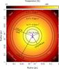 |
Fig. 11 Schematic view of the region of the clump and the typical temperatures traced by different molecules. This represents a clump with the typical properties traced by the different molecules, as observed in this work (cf. Fig. 5). The circles indicate the approximate radius at the median temperature traced by the species marked near to it (cf. Table 6), according to the colourscale. CO appears twice as it traces the outskirts of clumps when the temperature in the inner region is below 25 K, and the bulk of the dense gas when the temperature is above this threshold (see text). |
7.3. Dependence of temperature on the L/M ratio: an evolutionary sequence
Inspecting the relation between temperature and L/M ratio (Fig. 10) and using the classification defined for the TOP100 we identify three intervals in the luminosity-to-mass ratio, corresponding to different stages.
For  the derived gas temperatures depend only weakly on the ratio, or remains constant. In this interval, only 70w and IRw sources are present. Depending on the tracer used, for
  the relation between the temperature and the luminosity-to-mass ratio becomes steeper, revealing the direct correlation between these quantities in this regime, and showing that thermal feedback of the young stellar objects is now influencing the entire clump.
A threshold is identified above which hot cores begin to appear, for  . In this work we define a hot core as a source that was detected in the J = 19 → 18 line series of CH3CN and/or in the νt = 1 band of methanol. The fit results described in Sects. 6.2 and 6.3 indicate that hot gas with T ≳ 150 K must be present in these sources.
In the TOP100 37 objects fulfil these criteria, mainly in the IRb and Hii classes. The presence of a hot core is reported in Tables A.5 and A.8. There is a very good correspondence between the two tracers, with only one clump detected in CH3CN not detected in CH3OH (AGAL305.209+00.206 was not observed in methanol) and three sources detected in CH3OH, but not in acetonitrile, due to the contamination of CCH. As for the other tracers, the detection rate increases with evolution: no 70w source is detected, 20% of IRw clumps, 41% of IRb and 82% of Hii are found to harbour a hot core. Clearly, hot molecular gas is still present in the expanding envelopes of compact Hii regions, whose high opacity shields it from the ionising photons of the central source. The higher detection rate is likely a combination of a larger volume of gas significantly heated by the young stellar objects and multiple unresolved sources. The temperature in the envelope from CH3CN and CH3CCH of the 19 sources that host a hot core, but do not show radio-continuum emission yet, is marginally larger than that found in the remaining IRb, possibly suggesting that these clumps are more evolved.
The position of the sources with  in a M−L plot, as well as their bolometric luminosities, indicate that the first intermediate- or high-mass ZAMS stars have appeared, as discussed also in Molinari et al. (2016). Further evidence that this change is caused by the substantial heating from luminous ZAMS stars comes from the work of Urquhart et al. (2013a,b, 2014c), investigating in detail the properties of ATLASGAL sources associated with methanol masers and UCHii regions: from Fig. 21 in Urquhart et al. (2014c) it appears evident that massive YSOs and UCHii are consistent with this value in L/M.
Finally, for L/M values in excess of  Hii regions become predominant, marking the point where the dissipation of the parental clump starts to dominate.
7.4. Emitting regions and qualitative comparison with chemical models
In Sect. 6.2 we find that acetonitrile is characterised by two distinct components, one warm and extended and the other hot and compact, showing that this species is not tracing exclusively the gas in the immediate surroundings of high-mass young stellar objects, in agreement with the findings for NGC 7538 IRS9 by Öberg et al. (2013). CH3CN is therefore not a pure hot molecule, as usually assumed (e.g. Bisschop et al. 2007). As for the origin of the extended emission, astrochemical models predict a significant abundance of acetonitrile in warm gas, following the release of HCN from grains, leading to the gas-phase formation of CH3CN, for T ≳ 30 K (Garrod et al. 2008). If CH3CN is formed in the gas phase after evaporation of HCN from dust grains, the temperature traced by acetonitrile should show a minimum above the evaporation temperature of HCN. As discussed in Sect. 7.2, such a threshold effect is seen in Figs. 5 and 10; excluding two detected 70w sources, all clumps have temperature in excess of 20–30 K, which also corresponds to a threshold in L/M ~ 2 L⊙/M⊙. This minimum average T for the warm component falls below the models predictions, possibly indicating a lower evaporation temperature for HCN or a different desorption mechanism. The observations reported in this work are consistent with the predictions of the chemical models concerning the presence of an early and a late abundance peaks, characterising an extended warm component and the hot core, respectively. The measured median abundances of acetonitrile are a factor of ~ 5–10 higher than predicted by Garrod et al. (2008, we consider models with a medium warm-up timescale for this comparison), and their ratio is consistent with the model. Considering the uncertainties in the model and in the observations, predicted and observed abundances for CH3CN are in broad agreement.
Gratier et al. (2013) argue that bright acetonitrile lines can be associated with photon-dominated regions (PDRs), using deep spectra of the Horsehead Nebula taken at the DCO+ and HCO emission peaks, associated with dense, relatively cold gas and the PDR, respectively. The authors find abundances 30 times larger in the diffuse and UV-illuminated gas than in the dense core, concluding that the detection of CH3CN does not automatically imply high-densities. PDRs are associated with strong emission of polycyclic aromatic hydrocarbons (PAHs), which have strong bands at 8 μm. Using the fluxes at this wavelength from the SEDs, taken from König et al. (2017), we can verify whether the extended component is coming from PDRs, rather than warm, dense gas in the envelope, passively heated by the forming high-mass stars. If this were the case, a correlation should exist between eight micron fluxes and integrated line fluxes. Spearman’s and Kendall’s correlation tests reveal no correlation among these two quantities; a stronger correlation is found between the line flux and the bolometric luminosity of the source (ρ = 0.4, τ = 0.3, with p-values below 5 × 10⁻⁴), dominated by the high-mass YSOs, indicating that passive heating of the envelope is connected to the presence of acetonitrile in the gas phase.
Leurini et al. (2007b) show that to effectively populate the CH3OH torsionally-excited states radiative pumping is required. The necessity of an intense radiation field to excite these transitions makes them reliable tracers of hot cores that need the radiative and mechanical feedback from nascent high-mass YSOs. The energy of the first torsionally-excited transitions of methanol corresponds to a wavelength range of ~ 20−35 μm. If the photons at this wavelength are responsible for the excitation of the νt = 1 band at ~ 337 GHz band, and CH3OH, νt = 1 is thermalised with the radiation, an increase in the luminosity in the previously mentioned wavelength range leads to a higher temperature, as traced by these transitions. The closest measured continuum fluxes are those of WISE, MIPSGAL and MSX (21–24μm), and a Spearman test demonstrates that the temperature of the hot methanol component is more strongly correlated with the luminosity at these wavelengths, than with the bolometric luminosity of the source (ρ ~ 0.55 and ρ ~ 0.65, respectively, see Fig. 12). In contrast, high-excitation transitions from CH3CN are more tightly correlated with Lbol, suggesting that passive heating plays a more important role in this case. To conclude, the data indicate that methanol torsionally-excited lines and high-excitation transitions of CH3CN trace the hot core, but they are sensitive to the radiation field and to the passive heating from the massive YSO, respectively. For CH3OH, the observations are not in agreement with the models of Garrod et al. (2008). In cold gas, the abundance of CH3OH is much larger than predicted by the model (even considering subthermal excitation, see Sects. 6.3 and 7.2) and lower for the gas in the hot core, reflecting known problems related to desorption of this molecule and its overproduction on the grains (Garrod et al. 2008). However, in the hot gas, the measured abundance is consistent with the reduced ice abundance models described in Garrod et al. (2008).
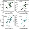 |
Fig. 12 Relations between the temperature of the hot components of CH3CN and CH3OH, and the bolometric- or 22 μm luminosity. In the top right corner of each panel the Spearman ρ is indicated. |
Our results indicate that the emitting region of CH3CCH is extended, and that it traces predominantly cold and warm gas in the envelope; as discussed in Sect. 6.1, we see no indications for a hot component suggesting a strong increase in abundance in hot cores, in contrast to CH3CN and CH3OH. A jump in abundance at temperatures higher than ≈20 K, analogous to CO, is also excluded by the gradual, regular increase in temperature observed from the ECDFs (cf. Fig. 9 and Sect. 7.3). For temperatures lower than this value, the possibility remains that methyl acetylene is mostly locked in grains. The extended nature of the emitting region and the absence of a strong jump in abundance for CH3CCH in hot gas is confirmed by interferometric observations of a small sample of high-mass star-forming regions in Öberg et al. (2013) and Fayolle et al. (2015). These works find that only a minor fraction (10–15%) of the single-dish line flux is recovered by interferometric data on scales of 4″, showing that most of the emission is originated in the envelope, also for high-excitation lines. A strong debate is ongoing in literature about how CH3CCH is formed, focusing on whether or not surface chemistry is necessary to explain the observed abundances of this species (e.g. Occhiogrosso et al. 2013; Hickson et al. 2016). We find that the detection rate of CH3CCH increases with evolutionary class, but we find no correlation between the temperature traced by methyl acetylene and its abundance, even when considering only sources with distances below 6 kpc, which would indicate a progressively more efficient evaporation from the grains due to the warm-up. This finding is in contrast with the results form Miettinen et al. (2006), but is based on a much larger number of sources. Therefore, if methyl acetylene is formed onto dust grains, it needs efficient routes of formation at low temperatures, such as the progressive hydrogenation reactions of C3 proposed by Hickson et al. (2016), as well as desorption mechanisms able to release a significant quantity of CH3CCH already for T ~ 20 K, to explain the scales and temperatures traced. Because no clear jump in abundance is seen in hot cores for this species also when the mantle is sublimated, only a small quantity of methyl acetylene must remain in the ice when a temperature of ~ 110 K is reached, either due to reprocessing or nearly complete sublimation at lower temperatures.
Giannetti et al. (2013) previously compared NH3 (1, 1) and (2, 2) emission with dust continuum for a sample of massive clumps, using data with comparable spatial resolution. In their maps the emitting regions of these tracers are very similar, and the temperatures are closely related. An extended emitting region for ammonia is in agreement with the properties derived from this species in the TOP100.
7.5. Reliability of CH3CN as a thermometer
In the previously-mentioned study of the Horsehead nebula, Gratier et al. (2013) find that CH3CN is subthermally excited with relevant implications for the derivation of column densities. The authors compare results from large velocity gradient models with traditional rotational diagrams distinguishing three regimes: LTE, moderate- and strong subthermal excitation. The volume densities to have 3 mm transitions in LTE should be of the order of a few 105 cm-3, whereas nH2 ≳ 4 × 104 cm-3 is sufficient to enter the regime of moderate subthermal excitation, for which the ratio of different K lines is still a good indicator of TK. This is of the order of the median volume density averaged along the line of sight for the TOP100. Independent tests performed with RADEX (van der Tak et al. 2007) confirm that ~ 104 cm-3 is sufficient to obtain reliable estimates of TK in this sample. The tight correlation between temperatures derived with CH3CN and CH3CCH give additional support to the idea that acetonitrile is a good thermometer in massive and dense clumps.
The J = 19 → 18 lines have a much higher critical density, however; the high temperatures required to excite these lines ensure that the emission comes predominantly from the hot core, where densities are much higher (≳107−8 cm-3, Garrod & Widicus Weaver 2013), again providing a reliable temperature probe for these regions.
Although the derived temperatures are reliable, column densities may be underestimated by a factor of a few, according to the discussion in Gratier et al. (2013).
7.6. Evolution of linewidths and volume densities
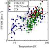 |
Fig. 13 Relation between temperature and line FWHM for CH3CN, CH3CCH and CO. The solid line indicates a mach number of 4. |
The forming stars continuously inject turbulence in the surrounding medium through outflows and winds. This leads to a local increase of the turbulent linewidth. Thus, as time passes and temperature increases, lines also become broader. Figure 13 shows that for CH3CN, CH3CCH, and C17O the measured gas temperatures also correlate with linewidths, that are always supersonic. CH3CN and CH3CCH linewidths are less contaminated by external layers in the envelope, and have a steeper dependence on the temperatures, becoming progressively more supersonic. The linewidths can also be broadened by infall motions: Wyrowski et al. (2016) use ammonia absorption to investigate the presence of infall in a sample of high-mass star-forming regions, finding that 72% of the sources show infall signatures and that the associated velocity is 3–30% of the free-fall value. Assuming a typical 10% of the free-fall velocity, we obtain an infall velocity of ≈0.3 km s-1 for the clumps in the TOP100, which has a negligible effect in terms of broadening. Hajigholi et al. (2016), however, show that in the inner regions of the envelope the infall proceeds with a velocity 0.4–0.7 of the free-fall value, which is also in line with a progressive broadening of the linewidth on smaller scales.
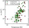 |
Fig. 14 Relation between volume density of molecular hydrogen at the peak of submm emission and temperature. This relation also shows that nH2 increases with evolution. |
Figure 14 illustrates that a relation exists between the temperature in the inner part of the envelope and the volume density of molecular hydrogen, calculated at the peak of continuum emission as nH2 = NH2/ 2R, where R is the source radius, as measured from dust. Following the discussion in Sect. 7.3, we deduce that the density in the central part of the source increases with evolution, due to the progressive accumulation of material at the bottom of the clump potential well.
These trends lend further support to the statistical validity of the evolutionary schemes analysed in this work.
7.7. Gravitational stability: best tracers
The virial stability of the clumps in the TOP100 was discussed in detail in Giannetti et al. (2014), and successively re-analised in light of the more accurate masses from the SED fit (König et al. 2017), using C17O (3–2) to derive linewidths. In this work we compared several molecular tracers; depending on which species is used to measure the linewidth, variations of a factor of ~ 2 are found in the median values for the FWHM in cold and warm gas. As a consequence, the virial mass varies of a factor of 4, as it depends on the square power of the linewidth, an uncertainty that has to be added to those for size and density profile.
Our results show that when investigating the stability of whole clumps, methyl acetylene is the most reliable tracer, as it comes from the dense part of the clump envelope, similar to that traced by dust continuum; CH3CCH also show no strong jumps in abundance across the evolutionary sequence. C17O (3–2) linewidths are in general well correlated with those of CH3CCH, however, it tends to slightly overestimate the linewidths in cold sources. Therefore, this transition also allows to reliably derive virial masses, except in the earliest evolutionary stages. CH3CN is more appropriate for the region surrounding the high-mass YSOs, and shows linewidths that are, on average, a factor 1.5 larger than those measured with methyl acetylene, due to its sharp variations in abundance connected to star-formation activity. The FWHM measured by the low-excitation methanol lines have very little correlation with clump properties, and are likely strongly influenced by the presence of outflows (cf. Leurini et al. 2016). Therefore, they are not reliable for this kind of analysis. The linewidths of methanol torsionally-excited lines and from CH3CN (19–18) are well correlated, and both these species can be used to test the stability of the hot core, provided that a measure of the mass and of the emitting region is available.
8. Conclusions and summary
The physical conditions traced by several commonly-used tracers were compared for the TOP100, a representative sample of high-mass star-forming regions in the disk of our Galaxy, identifying the most reliable probes for the envelope and for hot cores.
 |
Fig. 15 Simplified representation of the different phases identified for the TOP100, summarising our results. The colourscale indicates the progressive warm-up of the clump around a young stellar object. The physical processes dominating in the corresponding interval of L/M are also shown. |
The use of this sample to study the physical conditions of the gas and investigate whether the common paradigms used to classify high-mass star-forming regions in terms of evolution are consistent with the expected warm-up in time. From the comparison of the different tracers we find that they can probe widely different volumes of gas and physical properties (cf. Fig. 11), spanning temperatures between ~ 10 K and ~ 300 K, and linewidths in the range 1–15 km s-1. A major role in this sense is played by the specific chemistry of each species (formation routes, depletion, role of surface chemistry and evaporation from grains, etc.), which also influences their sensitivity to the warm-up process. In detail, CH3CCH show no significant jump in abundance and has narrow linewidths, indicating that it is tracing the dense and relatively quiescent material in the envelope. CH3CN is not exclusively a hot core tracer, but it is abundant in warm gas, associated with star-forming clumps as well. Because of its chemical properties, this molecule is an efficient tracer of the warm-up process, from its beginning to the development of a hot core. CH3OH traces both hot cores and cold gas, but it is a reliable probe of temperature only in the first case. C17O is a fair probe of physical conditions, especially for evolved sources, but the uncertainties are much larger when compared to those obtained by methyl acetylene and acetonitrile. NH3 is not a good tracer of warm-up when using only the (1, 1) and (2, 2) inversion transitions.
The detection of torsionally-excited methanol and high-excitation CH3CN lines (J = 19 → 18 was used in this work) implies temperatures in excess of 150 K, presenting an easy way to identify hot cores. CH3OH νt = 1 levels are pumped by IR radiation from high-mass YSOs, whereas the CH3CN (19–18) line series is excited by collision. The negligible contamination of cold and warm gas to high-J and high-K lines of acetonitrile and to torsionally-excited lines of methanol make these transitions suitable to study the kinematics of the hot gas in the immediate surroundings of young stellar objects.
We compared the abundance of CH3CN and CH3OH with those predicted by the models described in Garrod et al. (2008). The hot core and envelope abundances for CH3CN are ~ 4 × 10⁻¹⁰ and 10-7, respectively; the abundance ratio in hot and warm gas is in broad agreement with the models. On the contrary, the abundance of CH3OH is much larger than predicted by the model for cold gas; for hot gas, CH3OH abundance is consistent with the predictions of Garrod et al. (2008) only when using the reduced ice abundance models.
Linking these findings with potential ways of defining an evolutionary sequence, we conclude that both the L/M ratio and the classification based on the IR and radio continuum properties of the source define a statistically valid evolutionary sequence, demonstrated by the progressive warm-up of the gas in the clump, as well as the increase in linewidths and volume density of molecular hydrogen. The different phases of the process can thus be separated as follows (Fig. 15):
-
: material is still being accumulated and compressed (see Sect. 7.2, 7.3 and the discussion in Molinari et al. 2016), as suggested by the low detection rate of CH3CN and, to a lower extent, CH3CCH. This is in agreement with the higher volume density needed to excite acetonitrile lines, and with the subthermal excitation of CO. In this interval of L/M ratios (proto-)stellar activity is just starting: only two sources (17%) are associated with methanol masers, and a limited fraction show weak IR emission. We are therefore observing the compression and collapse phases.
-
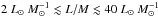 : the young stellar objects accrete material and grow in mass, reaching the ZAMS at
  . When they begin to burn hydrogen, they significantly increase their feedback on the surrounding environment (see Sect. 7.3); hot cores and compact Hii regions start to appear around this value in L/M as well. After reaching the ZAMS the young stellar object is still accreting mass. The fraction of sources associated with a maser increases substantially in this interval of L/M: it is 33% below and 80% above this threshold.
 -
 : radio continuum becomes common, marking the point where dissipation starts to dominate. The detection rate of methanol masers remains stable at ~ 80%.
These findings constitute the foundations for a complete study of the process of high-mass star formation throughout our Galaxy: it is now possible to identify virtually all massive star-forming regions in the Galaxy (as seen by ATLASGAL, Urquhart et al., in prep.) and classify them in terms of evolution, as an example, to investigate the timescales of the process and the statistical lifetime of each phase.
A more detailed description of these methods is given in the PyMC documentation https://pymc-devs.github.io/pymc/index.html
We used a Gaussian kernel, with a bandwidth selected with Kullback-Leibler cross-validation (Hurvich et al. 1998), and a local constant estimator.
Acknowledgments
This work was carried out within the Collaborative Research Council 956, sub-project A6, funded by the Deutsche Forschungsgemeinschaft (DFG). This paper is based on data acquired with the Atacama Pathfinder EXperiment (APEX). APEX is a collaboration between the Max Planck Institute for Radioastronomy, the European Southern Observatory, and the Onsala Space Observatory. This work also make use of observations carried out with the Mopra telescope and with the IRAM 30 m Telescope, under project number 181-10. The Mopra radio telescope is part of the Australia Telescope National Facility which is funded by the Australian Government for operation as a National Facility managed by CSIRO. IRAM is supported by INSU/CNRS (France), MPG (Germany) and IGN (Spain). T.Cs. acknowledges support from the DFG via the SPP (priority programme) 1573 “Physics of the ISM”. This research made use of Astropy, a community-developed core Python package for Astronomy (Astropy Collaboration et al. 2013, http://www.astropy.org), of NASA’s Astrophysics Data System, of Matplotlib (Hunter 2007), and of the Veusz plotting package (http://home.gna.org/veusz/). We thank the anonymous referee for their constructive and useful report that allowed to improve the clarity of this work.
References
- Askne, J., Hoglund, B., Hjalmarson, A., & Irvine, W. M. 1984, A&A, 130, 311 [NASA ADS] [Google Scholar]
- Astropy Collaboration, Robitaille, T. P., Tollerud, E. J., et al. 2013, A&A, 558, A33 [NASA ADS] [CrossRef] [EDP Sciences] [Google Scholar]
- Bacmann, A., Lefloch, B., Ceccarelli, C., et al. 2002, A&A, 389, L6 [NASA ADS] [CrossRef] [EDP Sciences] [Google Scholar]
- Bergin, E. A., Goldsmith, P. F., Snell, R. L., & Ungerechts, H. 1994, ApJ, 431, 674 [NASA ADS] [CrossRef] [Google Scholar]
- Beuther, H., Schilke, P., Menten, K. M., et al. 2002, ApJ, 566, 945 [NASA ADS] [CrossRef] [Google Scholar]
- Beuther, H., Zhang, Q., Bergin, E. A., et al. 2007, A&A, 468, 1045 [NASA ADS] [CrossRef] [EDP Sciences] [Google Scholar]
- Bisschop, S. E., Jørgensen, J. K., van Dishoeck, E. F., & de Wachter, E. B. M. 2007, A&A, 465, 913 [NASA ADS] [CrossRef] [EDP Sciences] [Google Scholar]
- Breen, S. L., Fuller, G. A., Caswell, J. L., et al. 2015, MNRAS, 450, 4109 [NASA ADS] [CrossRef] [Google Scholar]
- Brown, L. D., Cai, T. T., & DasGupta, A. 2001, Stat. Sci., 16, 101 [Google Scholar]
- Carey, S. J., Noriega-Crespo, A., Mizuno, D. R., et al. 2009, PASP, 121, 76 [NASA ADS] [CrossRef] [Google Scholar]
- Cesaroni, R. 2005, in Massive Star Birth: A Crossroads of Astrophysics, eds. R. Cesaroni, M. Felli, E. Churchwell, & M. Walmsley, IAU Symp., 227, 59 [Google Scholar]
- Comito, C., Schilke, P., Phillips, T. G., et al. 2005, ApJS, 156, 127 [NASA ADS] [CrossRef] [Google Scholar]
- Contreras, Y., Schuller, F., Urquhart, J. S., et al. 2013, A&A, 549, A45 [NASA ADS] [CrossRef] [EDP Sciences] [Google Scholar]
- Csengeri, T., Urquhart, J. S., Schuller, F., et al. 2014, A&A, 565, A75 [NASA ADS] [CrossRef] [EDP Sciences] [Google Scholar]
- Csengeri, T., Leurini, S., Wyrowski, F., et al. 2016, A&A, 586, A149 [NASA ADS] [CrossRef] [EDP Sciences] [Google Scholar]
- Elia, D., Molinari, S., Fukui, Y., et al. 2013, ApJ, 772, 45 [NASA ADS] [CrossRef] [Google Scholar]
- Fayolle, E. C., Öberg, K. I., Garrod, R. T., van Dishoeck, E. F., & Bisschop, S. E. 2015, A&A, 576, A45 [NASA ADS] [CrossRef] [EDP Sciences] [Google Scholar]
- Fontani, F., Cesaroni, R., Caselli, P., & Olmi, L. 2002, A&A, 389, 603 [NASA ADS] [CrossRef] [EDP Sciences] [Google Scholar]
- Gadhi, J., Lahrouni, A., Legrand, J., & J., D. 1995, J. Chim. Phys., 92, 1984 [CrossRef] [EDP Sciences] [Google Scholar]
- Garrod, R. T., Weaver, S. L. W., & Herbst, E. 2008, ApJ, 682, 283 [NASA ADS] [CrossRef] [Google Scholar]
- Garrod, R. T., & Widicus Weaver, S. L. 2013, Chem. Rev., 113, 8939 [Google Scholar]
- Gelman, A., Carlin, J., Stern, H., & Rubin, D. 2003, Bayesian Data Analysis, Second Edition, Chapman & Hall/CRC Texts in Statistical Science (Taylor & Francis) [Google Scholar]
- Geweke, J. 1992a, in Bayesian Statistics 4, eds. J. M. Bernardo, J. Berger, A. P. Dawid, & J. F. M. Smith (Oxford: Oxford University Press), 169 [Google Scholar]
- Geweke, J. 1992b, in Bayesian Statistics 4, eds. J. M. Bernardo, J. Berger, A. P. Dawid, & J. F. M. Smith (Oxford: Oxford University Press), 625 [Google Scholar]
- Giannetti, A., Brand, J., Sánchez-Monge, Á., et al. 2013, A&A, 556, A16 [NASA ADS] [CrossRef] [EDP Sciences] [Google Scholar]
- Giannetti, A., Wyrowski, F., Brand, J., et al. 2014, A&A, 570, A65 [NASA ADS] [CrossRef] [EDP Sciences] [Google Scholar]
- Gibb, E. L., Whittet, D. C. B., Boogert, A. C. A., & Tielens, A. G. G. M. 2004, ApJS, 151, 35 [NASA ADS] [CrossRef] [PubMed] [Google Scholar]
- Gratier, P., Pety, J., Guzmán, V., et al. 2013, A&A, 557, A101 [NASA ADS] [CrossRef] [EDP Sciences] [Google Scholar]
- Green, J. A., Caswell, J. L., Fuller, G. A., et al. 2009, MNRAS, 392, 783 [NASA ADS] [CrossRef] [Google Scholar]
- Haario, H., Saksman, E., & Tamminen, J. 2001, Bernoulli, 7, 223 [CrossRef] [MathSciNet] [Google Scholar]
- Hajigholi, M., Persson, C. M., Wirström, E. S., et al. 2016, A&A, 585, A158 [NASA ADS] [CrossRef] [EDP Sciences] [Google Scholar]
- Hastings, W. K. 1970, Biometrika, 57, 97 [Google Scholar]
- Hayfield, T., & Racine, J. S. 2008, J. Stat. Software, 27 [Google Scholar]
- Heyer, M., Gutermuth, R., Urquhart, J. S., et al. 2016, A&A, 588, A29 [NASA ADS] [CrossRef] [EDP Sciences] [Google Scholar]
- Hickson, K. M., Wakelam, V., & Loison, J.-C. 2016, Mol. Astrophys., 3, 1 [NASA ADS] [CrossRef] [Google Scholar]
- Hoare, M. G., Purcell, C. R., Churchwell, E. B., et al. 2012, PASP, 124, 939 [NASA ADS] [CrossRef] [Google Scholar]
- Hosokawa, T., & Omukai, K. 2009, ApJ, 691, 823 [NASA ADS] [CrossRef] [Google Scholar]
- Hunter, J. D. 2007, Comput. Sci. Eng., 9, 90 [Google Scholar]
- Hurvich, C. M., Simonoff, J. S., & Tsai, C. 1998, J. Roy. Stat. Soc.: Ser. B (Statistical Methodology), 60, 271 [CrossRef] [Google Scholar]
- Jaynes, E., & Bretthorst, G. 2003, Probability Theory: The Logic of Science (Cambridge University Press) [Google Scholar]
- Kauffmann, J., & Pillai, T. 2010, ApJ, 723, L7 [NASA ADS] [CrossRef] [Google Scholar]
- Kennicutt, R. C., & Evans, N. J. 2012, ARA&A, 50, 531 [NASA ADS] [CrossRef] [Google Scholar]
- Kim, W.-J., Wyrowski, F., Urquhart, J. S., Menten, K. M., & Csengeri, T. 2017, A&A, 602, A37 [NASA ADS] [CrossRef] [EDP Sciences] [Google Scholar]
- Klein, T., Ciechanowicz, M., Leinz, C., et al. 2014, IEEE Trans. Terahertz Sci. Technol., 4, 588 [NASA ADS] [CrossRef] [Google Scholar]
- König, C., Urquhart, J. S., Csengeri, T., et al. 2017, A&A, 599, A139 [NASA ADS] [CrossRef] [EDP Sciences] [Google Scholar]
- Kuiper, T. B. H., Kuiper, E. N. R., Dickinson, D. F., Turner, B. E., & Zuckerman, B. 1984, ApJ, 276, 211 [NASA ADS] [CrossRef] [Google Scholar]
- Leurini, S., Schilke, P., Menten, K. M., et al. 2004, A&A, 422, 573 [NASA ADS] [CrossRef] [EDP Sciences] [Google Scholar]
- Leurini, S., Beuther, H., Schilke, P., et al. 2007a, A&A, 475, 925 [NASA ADS] [CrossRef] [EDP Sciences] [Google Scholar]
- Leurini, S., Schilke, P., Wyrowski, F., & Menten, K. M. 2007b, A&A, 466, 215 [NASA ADS] [CrossRef] [EDP Sciences] [Google Scholar]
- Leurini, S., Codella, C., Cabrit, S., et al. 2016, A&A, 595, L4 [NASA ADS] [CrossRef] [EDP Sciences] [Google Scholar]
- Mac Low, M.-M., & Klessen, R. S. 2004, Rev. Mod. Phys., 76, 125 [NASA ADS] [CrossRef] [Google Scholar]
- Maret, S., Hily-Blant, P., Pety, J., Bardeau, S., & Reynier, E. 2011, A&A, 526, A47 [NASA ADS] [CrossRef] [EDP Sciences] [Google Scholar]
- Miettinen, O., Harju, J., Haikala, L. K., & Pomrén, C. 2006, A&A, 460, 721 [NASA ADS] [CrossRef] [EDP Sciences] [Google Scholar]
- Molinari, S., Pezzuto, S., Cesaroni, R., et al. 2008, A&A, 481, 345 [NASA ADS] [CrossRef] [EDP Sciences] [Google Scholar]
- Molinari, S., Swinyard, B., Bally, J., et al. 2010, PASP, 122, 314 [NASA ADS] [CrossRef] [Google Scholar]
- Molinari, S., Merello, M., Elia, D., et al. 2016, ApJ, 826, L8 [Google Scholar]
- Muenter, J. S., & Laurie, V. W. 1980, J. Chem. Phys., 45, 855 [NASA ADS] [CrossRef] [Google Scholar]
- Müller, H. S. P., Thorwirth, S., Roth, D. A., & Winnewisser, G. 2001, A&A, 370, L49 [NASA ADS] [CrossRef] [EDP Sciences] [Google Scholar]
- Navarete, F., Leurini, S., Giannetti, A., et al. 2017, A&A, submitted [Google Scholar]
- Öberg, K. I., Boamah, M. D., Fayolle, E. C., et al. 2013, ApJ, 771, 95 [NASA ADS] [CrossRef] [Google Scholar]
- Occhiogrosso, A., Viti, S., & Balucani, N. 2013, MNRAS, 432, 3423 [NASA ADS] [CrossRef] [Google Scholar]
- Parzen, E. 1962, Ann. Math. Stat., 33, 1065 [NASA ADS] [CrossRef] [MathSciNet] [Google Scholar]
- Patil, A., Huard, D., & Fonnesbeck, C. 2010, J. Stat. Software, 35, 1 [Google Scholar]
- Pickett, H. M., Poynter, R. L., Cohen, E. A., et al. 1998, J. Quant. Spectr. Rad. Transf., , 60, 883 [Google Scholar]
- Price, S. D., Egan, M. P., Carey, S. J., Mizuno, D. R., & Kuchar, T. A. 2001, AJ, 121, 2819 [NASA ADS] [CrossRef] [Google Scholar]
- Purcell, C. R., Hoare, M. G., Cotton, W. D., et al. 2013, ApJS, 205, 1 [NASA ADS] [CrossRef] [Google Scholar]
- Raftery, A. E., & Lewis, S. M. 1995, in Practical Markov chain Monte Carlo, eds. W. R. Gilks, & D. J. Spiegelhalter (Chapman and Hall), 115 [Google Scholar]
- Remijan, A., Sutton, E. C., Snyder, L. E., et al. 2004, ApJ, 606, 917 [NASA ADS] [CrossRef] [Google Scholar]
- Roberts, J. F., Rawlings, J. M. C., Viti, S., & Williams, D. A. 2007, MNRAS, 382, 733 [NASA ADS] [CrossRef] [Google Scholar]
- Rosenblatt, M. 1956, Ann. Math. Stat., 27, 832 [CrossRef] [MathSciNet] [Google Scholar]
- Rowan-Robinson, M. 1980, ApJS, 44, 403 [NASA ADS] [CrossRef] [Google Scholar]
- Sanna, A., Cesaroni, R., Moscadelli, L., et al. 2014, A&A, 565, A34 [NASA ADS] [CrossRef] [EDP Sciences] [Google Scholar]
- Saraceno, P., Andre, P., Ceccarelli, C., Griffin, M., & Molinari, S. 1996, A&A, 309, 827 [NASA ADS] [Google Scholar]
- Scannapieco, C., Wadepuhl, M., Parry, O. H., et al. 2012, MNRAS, 423, 1726 [Google Scholar]
- Scholz, F. W., & Stephens, M. A. 1987, J. Amer. Stat. Assoc., 82, 918 [Google Scholar]
- Schuller, F., Menten, K. M., Contreras, Y., et al. 2009, A&A, 504, 415 [NASA ADS] [CrossRef] [EDP Sciences] [Google Scholar]
- Smith, I. W. M., Herbst, E., & Chang, Q. 2004, MNRAS, 350, 323 [NASA ADS] [CrossRef] [Google Scholar]
- Urquhart, J. S., Hoare, M. G., Lumsden, S. L., Oudmaijer, R. D., & Moore, T. J. T. 2008, in Massive Star Formation: Observations Confront Theory, eds. H. Beuther, H. Linz, & T. Henning, ASP Conf. Ser., 387, 381 [Google Scholar]
- Urquhart, J. S., Hoare, M. G., Purcell, C. R., et al. 2009, A&A, 501, 539 [NASA ADS] [CrossRef] [EDP Sciences] [Google Scholar]
- Urquhart, J. S., Moore, T. J. T., Schuller, F., et al. 2013a, MNRAS, 431, 1752 [Google Scholar]
- Urquhart, J. S., Thompson, M. A., Moore, T. J. T., et al. 2013b, MNRAS, 435, 400 [NASA ADS] [CrossRef] [Google Scholar]
- Urquhart, J. S., Csengeri, T., Wyrowski, F., et al. 2014a, A&A, 568, A41 [NASA ADS] [CrossRef] [EDP Sciences] [Google Scholar]
- Urquhart, J. S., Figura, C. C., Moore, T. J. T., et al. 2014b, MNRAS, 437, 1791 [NASA ADS] [CrossRef] [Google Scholar]
- Urquhart, J. S., Moore, T. J. T., Csengeri, T., et al. 2014c, MNRAS, 443, 1555 [NASA ADS] [CrossRef] [Google Scholar]
- van der Tak, F. F. S., van Dishoeck, E. F., & Caselli, P. 2000, A&A, 361, 327 [NASA ADS] [Google Scholar]
- van der Tak, F. F. S., Black, J. H., Schöier, F. L., Jansen, D. J., & van Dishoeck, E. F. 2007, A&A, 468, 627 [NASA ADS] [CrossRef] [EDP Sciences] [Google Scholar]
- Viti, S., Collings, M. P., Dever, J. W., McCoustra, M. R. S., & Williams, D. A. 2004, MNRAS, 354, 1141 [NASA ADS] [CrossRef] [Google Scholar]
- Walsh, A. J., Burton, M. G., Hyland, A. R., & Robinson, G. 1998, MNRAS, 301, 640 [NASA ADS] [CrossRef] [Google Scholar]
- Wienen, M., Wyrowski, F., Schuller, F., et al. 2012, A&A, 544, A146 [NASA ADS] [CrossRef] [EDP Sciences] [Google Scholar]
- Wilner, D. J., Welch, W. J., & Forster, J. R. 1995, ApJ, 449, L73 [NASA ADS] [CrossRef] [Google Scholar]
- Wolfire, M. G., & Cassinelli, J. P. 1986, ApJ, 310, 207 [CrossRef] [Google Scholar]
- Wyrowski, F., Güsten, R., Menten, K. M., et al. 2016, A&A, 585, A149 [NASA ADS] [CrossRef] [EDP Sciences] [Google Scholar]
- Zhang, Q., Wang, K., Lu, X., & Jiménez-Serra, I. 2015, ApJ, 804, 141 [NASA ADS] [CrossRef] [Google Scholar]
- Zinnecker, H., & Yorke, H. W. 2007, ARA&A, 45, 481 [NASA ADS] [CrossRef] [Google Scholar]
Appendix A: Additional figures
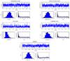 |
Fig. A.1 Example of trace plot (top), probability distribution function (bottom left), and autocorrelation plot (bottom right), for AGAL014.632–00.577 (for each parameter, indicated at the top of each panel). The plots refer to CH3CN. |
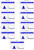 |
Fig. A.2 Example of trace plot (top), probability distribution function (bottom left), and autocorrelation plot (bottom right) for AGAL034.258+00.154 (for each parameter, indicated at the top of each panel). The plots refer to CH3CN. |
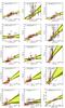 |
Fig. A.3 Correlations between temperatures as measured by different tracers. In each panel we include the best fit result as a blue solid line. The uncertainties due to the line parameters are indicated by the shaded region – dark- and light yellow for 68% and 95%, respectively. The intrinsic scatter in the relation is indicated by the dashed black lines. At the bottom right of the panels the Spearman correlation coefficient is shown. |
All Tables
Resulting p-values of Anderson-Darling tests for the three species considered in this work.
All Figures
|
Fig. 1 Simple schematic flow-chart of MCWeeds. The steps performed when using MCMCs are highlighted in blue and those for MAP or normal approximation in green. A more detailed description is given in the text. |
| In the text | |
|
Fig. 2 Example of the fit performed with MCWeeds for CH3CCH. The K components are indicated in green. The best fit model is shown in red. The source on the left is an IRw and the source on the right belong to Hii. |
| In the text | |
|
Fig. 3 Example of the fit performed with MCWeeds for CH3CN. The K components of CH3CN are indicated in green and those of CH313CN are indicated in blue. The best fit model is shown in red. The source on the left is an IRw and the source on the right belong to Hii. |
| In the text | |
|
Fig. 4 Example of the fit performed with MCWeeds for CH3OH. The best fit model is shown in red. The lines not reproduced by the model are contaminating species and are excluded from the spectral ranges used for the fit (cf. Table 2) The top panel show the results for an IRw source and the bottom panel for an Hii. The νt = 1 band is visible between ~ 337 500 and ~380 000 MHz. |
| In the text | |
|
Fig. 5 Empirical cumulative distribution functions for a) temperatures, b) line FWHMs, c) source diameter, and d) molecular column density. The different tracers and components are drawn with different colours, as indicated in the legend in the lower right corner of panel b). “CO” refers to properties obtained from C17O and C18O transitions from Giannetti et al. (2014), and NH3 properties are taken from Wienen et al. (2012). Dust properties from König et al. (2017) are included only in panels a) and c). |
| In the text | |
|
Fig. 6 Empirical cumulative distribution function for the abundance relative to molecular hydrogen. CH3CCH, and the hot and cool components of CH3CN and CH3OH are drawn with different colours, as indicated in panel b) of Fig. 5. |
| In the text | |
|
Fig. 7 Correlation between the temperature as measured by CH3CN and CH3CCH. All the other combinations between the tracers analysed are included in the online material in Fig. A. The best fit is shown as a blue solid line. The uncertainties due to the line parameters are indicated by the shaded region – dark- and light yellow for 68% and 95% HPD intervals, respectively. The intrinsic scatter in the relation is indicated by the dashed black lines. At the bottom right of the panels the Spearman correlation coefficient is indicated. |
| In the text | |
|
Fig. 8 Kernel density estimate of the probability density function, normalised to its maximum for displaying purposes, for the excitation temperature as traced by CO isotopologues. The thin lines represent the different classes: black – 70w, blue – IRw, red – IRb, and green – Hii. The thick black line refer to the entire TOP100 sample. |
| In the text | |
|
Fig. 9 Comparison between empirical cumulative distribution functions of the temperature for the four evolutionary classes defined for the TOP100. Each panel show one of the species analised in this work. The four evolutionary classes are indicated in a different colour, according to the legend shown in the lower right corner of panel c). The solid line at p = 0.5 shows the median of the distributions. |
| In the text | |
|
Fig. 10 L/M ratio vs. temperature. The black solid line indicates the line-of-sight- and beam-averaged temperature for a spherical clump model passively heated by a central object accounting for the total luminosity. The thick grey line shows the non-parametric regression of the data, with uncertainties indicated by the yellow-shaded area. |
| In the text | |
|
Fig. 11 Schematic view of the region of the clump and the typical temperatures traced by different molecules. This represents a clump with the typical properties traced by the different molecules, as observed in this work (cf. Fig. 5). The circles indicate the approximate radius at the median temperature traced by the species marked near to it (cf. Table 6), according to the colourscale. CO appears twice as it traces the outskirts of clumps when the temperature in the inner region is below 25 K, and the bulk of the dense gas when the temperature is above this threshold (see text). |
| In the text | |
|
Fig. 12 Relations between the temperature of the hot components of CH3CN and CH3OH, and the bolometric- or 22 μm luminosity. In the top right corner of each panel the Spearman ρ is indicated. |
| In the text | |
|
Fig. 13 Relation between temperature and line FWHM for CH3CN, CH3CCH and CO. The solid line indicates a mach number of 4. |
| In the text | |
|
Fig. 14 Relation between volume density of molecular hydrogen at the peak of submm emission and temperature. This relation also shows that nH2 increases with evolution. |
| In the text | |
|
Fig. 15 Simplified representation of the different phases identified for the TOP100, summarising our results. The colourscale indicates the progressive warm-up of the clump around a young stellar object. The physical processes dominating in the corresponding interval of L/M are also shown. |
| In the text | |
|
Fig. A.1 Example of trace plot (top), probability distribution function (bottom left), and autocorrelation plot (bottom right), for AGAL014.632–00.577 (for each parameter, indicated at the top of each panel). The plots refer to CH3CN. |
| In the text | |
|
Fig. A.2 Example of trace plot (top), probability distribution function (bottom left), and autocorrelation plot (bottom right) for AGAL034.258+00.154 (for each parameter, indicated at the top of each panel). The plots refer to CH3CN. |
| In the text | |
|
Fig. A.3 Correlations between temperatures as measured by different tracers. In each panel we include the best fit result as a blue solid line. The uncertainties due to the line parameters are indicated by the shaded region – dark- and light yellow for 68% and 95%, respectively. The intrinsic scatter in the relation is indicated by the dashed black lines. At the bottom right of the panels the Spearman correlation coefficient is shown. |
| In the text | |
Current usage metrics show cumulative count of Article Views (full-text article views including HTML views, PDF and ePub downloads, according to the available data) and Abstracts Views on Vision4Press platform.
Data correspond to usage on the plateform after 2015. The current usage metrics is available 48-96 hours after online publication and is updated daily on week days.
Initial download of the metrics may take a while.