| Issue |
A&A
Volume 603, July 2017
|
|
|---|---|---|
| Article Number | A110 | |
| Number of page(s) | 16 | |
| Section | Astrophysical processes | |
| DOI | https://doi.org/10.1051/0004-6361/201629672 | |
| Published online | 18 July 2017 | |
Modified viscosity in accretion disks
Application to Galactic black hole binaries, intermediate mass black holes, and active galactic nuclei
1 Center for Theoretical Physics, Polish Academy of Sciences, Al. Lotnikow 32/46, 02-668 Warsaw, Poland
e-mail: This email address is being protected from spambots. You need JavaScript enabled to view it.
2 School of Physics, Huazhong University of Science and Technology, 430074 Wuhan, PR China
Received: 8 September 2016
Accepted: 13 April 2017
Abstract
Aims. Black holes (BHs) surrounded by accretion disks are present in the Universe at different scales of masses, from microquasars up to the active galactic nuclei (AGNs). Since the work of Shakura & Sunyaev (1973, A&A, 24, 337) and their α-disk model, various prescriptions for the heat-production rate are used to describe the accretion process. The current picture remains ad hoc due the complexity of the magnetic field action. In addition, accretion disks at high Eddington rates can be radiation-pressure dominated and, according to some of the heating prescriptions, thermally unstable. The observational verification of their resulting variability patterns may shed light on both the role of radiation pressure and magnetic fields in the accretion process.
Methods. We compute the structure and time evolution of an accretion disk, using the code GLADIS (which models the global accretion disk instability). We supplement this model with a modified viscosity prescription, which can to some extent describe the magnetisation of the disk. We study the results for a large grid of models, to cover the whole parameter space, and we derive conclusions separately for different scales of black hole masses, which are characteristic for various types of cosmic sources. We show the dependencies between the flare or outburst duration, its amplitude, and period, on the accretion rate and viscosity scaling.
Results. We present the results for the three grids of models, designed for different black hole systems (X-ray binaries, intermediate mass black holes, and galaxy centres). We show that if the heating rate in the accretion disk grows more rapidly with the total pressure and temperature, the instability results in longer and sharper flares. In general, we confirm that the disks around the supermassive black holes are more radiation-pressure dominated and present relatively brighter bursts. Our method can also be used as an independent tool for the black hole mass determination, which we confront now for the intermediate black hole in the source HLX-1. We reproduce the light curve of the HLX-1 source. We also compare the duration times of the model flares with the ages and bolometric luminosities of AGNs.
Conclusions. With our modelling, we justify the modified μ-prescription for the stress tensor τrφ in the accretion flow in microquasars. The discovery of the Ultraluminous X-ray source HLX-1, claimed to be an intermediate black hole, gives further support to this result. The exact value of the μ parameter, as fitted to the observed light curves, may be treated as a proxy for the magnetic field strength in the accretion flow in particular sources, or their states.
Key words: black hole physics / X-rays: binaries / X-rays: galaxies / accretion, accretion disks / hydrodynamics / instabilities
© ESO, 2017
1. Introduction
Accretion disks are ubiquitous in the astrophysical black holes (BHs) environment, and populate a large number of known sources. Black hole masses range from stellar mass black holes in X-ray binaries, through intermediate mass black holes (IMBHs), up to the supermassive blackholes in quasars and active galaxy centers (active galactic nuclei, AGNs). The geometrically thin, optically thick accretion disk that is described by the theory of Shakura and Sunyaev is probably most relevant for the high/soft spectral states of black hole X-ray binaries, as well as for some active galaxies, such as narrow line Seyfert 1s and numerous radio quiet quasars (Brandt et al. 1997; Peterson et al. 2000; Foschini et al. 2015). The basic theory of a geometrically thin stationary accretion is based on the simple albeit powerful α prescription for the viscosity in the accreting plasma, introduced by Shakura & Sunyaev (1973). This simple scaling of viscous stress with pressure is also reproduced in the more recent numerical simulations of magnetised plasmas (Hirose et al. 2006; Jiang et al. 2013; Mishra et al. 2016). However, the latter are still not capable of modelling the global dynamics, time variability, and radiation emitted in the cosmic sources, and hence cannot be directly adopted to fit the observations.
The global models, however, must go beyond the stationary model, as the time-dependent effects connected with non-stationary accretion are clearly important. In particular, a number of observational facts support the idea of a cyclic activity in the high-accretion-rate sources. One of the best studied examples is the microquasar GRS 1915+105, which in some spectral states exhibits cyclic flares of its X-ray luminosity, well fitted to the limit cycle oscillations of an accretion disk on timescales of tens or hundreds of seconds Taam et al. (1997), Belloni et al. (2000), Neilsen et al. (2011). Those heartbeat states are known since 1997, when the first XTE PCA observations of this source were published (Taam et al. 1997), while recently yet another microquasar of that type, IGR J17091-3624, was discovered (Revnivtsev et al. 2003; Kuulkers et al. 2003; Capitanio et al. 2009); heartbeat states were also found for this source (Altamirano et al. 2011b; Capitanio et al. 2012; Pahari et al. 2014; Janiuk et al. 2015). Furthermore, a sample of sources proposed in Janiuk & Czerny (2011) was suggested to undergo luminosity oscillations, possibly induced by the non-linear dynamics of the emitting gas. This suggestion was confirmed by the recurrence analysis of the observed time series, presented in Suková et al. (2016).
One possible driver of the non-linear process in the accretion disk is its thermal and viscous oscillation induced by the radiation pressure term; it can be dominant for high enough accretion rates in the innermost regions of the accretion disk, which are the hottest. The timescales of such oscillations depend on the black hole mass, and are on the order of tens to hundreds of seconds for stellar mass BH systems. For a typical supermassive black hole of 108M⊙, the process would require timescales of hundreds of years. Therefore, in active galactic nuclei (AGNs) we cannot observe the evolution under the radiation pressure instability directly. Nevertheless, statistical studies may shed some light on the sources’ evolution. For instance, the Giga-Hertz Peaked quasars (Czerny et al. 2009) have very compact sizes, which would directly imply their ages. In the case of a limit-cycle kind of evolution, these sources would in fact not be very young, but “reactivated”. Another observational hint is the shape of distortions or discontinuities in the radio structures. These structures may reflect the history of the central power source of a quasar, which has been through subsequent phases of activity and quiescence. An exemplary source of that kind, quasar FIRST J164311.3+315618, was studied in Kunert-Bajraszewska & Janiuk (2011), and found to exhibit multiple radio structures. Another class of objects, which are claimed to contain the BH accretion disk, are the Ultraluminous X-ray sources (ULXs). ULXs are a class of sources that have a luminosity larger than the Eddington one for the heaviest stellar-mass objects (> 1040 erg s-1). Therefore, ULXs are frequently claimed to contain accreting black holes with masses larger than the most massive stars and lower than AGNs (103−106M⊙ intermediate-mass black holes, IMBHs). An example object in this class is HLX-1, which is possibly the best known candidate for an IMBH (Farrell et al. 2009; Lasota et al. 2011; Servillat et al. 2011; Godet et al. 2012). This source is located near the spiral galaxy ESO 243-49 (Wiersema et al. 2010; Soria et al. 2013) with peak luminosity exceeding 1042 erg s-1. HLX-1 also exhibits periodic limit-cycle oscillations. During seven years of observations of its X-Ray variability, six significant bursts lasting a few tens of days have been noticed. The mass of the black hole inside HLX-1 is estimated at about 104−105M⊙ (Straub et al. 2014). In this work, we investigate a broad range of theoretical models of radiation-pressure-driven flares and prepare the results for easy confrontation with observational data. The appearance of the radiation pressure instability in hot parts of accretion disks can lead to significant outburst for all scales of the black hole mass. Temperature and heat production rate determine the outburst frequency and shape. Different effective prescriptions for turbulent viscosity affect the instability range and the outburst properties. Thus, by confronting the model predictions with observed flares, we can put constraints on those built-in assumptions.
The attractiveness of the radiation pressure instability as a mechanism to explain various phenomena across the whole black hole mass scale has been outlined by Wu et al. (2016). In the present paper we expand this work by making a systematic study showing how the model parameters modify the local stability curve and global disk behaviour. We expand the parameter space of the model and identify the key parameters characterising the data. We develop a convenient way to compare the models to the data by providing simple fits to model predictions for the parameters directly measurable from the data. This approach makes the dependence of the models on the parameters much more clear, and it allows for much easier comparison of the model with observational data.
2. Model
2.1. Radiation pressure instability
In the α-model of the accretion disk, the non-zero component τrφ of the stress tensor is assumed to be proportional to the total pressure. The latter includes the radiation pressure component, which scales with temperature as T4 and blows up in hot, optically thick disks for large accretion rates. In general, an adopted assumption about the dependence of the τrφ on the local disk properties leads to a specific prediction of the behaviour of the disk heating. This in turn affects the heating and cooling balance between the energy dissipation and radiative losses.
Such a balance, under the assumption of hydrostatic equilibrium, is calculated numerically with a closing equation for the locally dissipated flux of energy given by the black hole mass and global accretion rate. The local solutions of the thermal balance and structure of a stationary accretion disk at a given radius may be conveniently plotted in the form of a so-called stability curve of the shape S. Here, distinct points represent the annulus in a disk, with temperature and surface density determined by the accretion rate. For small accretion rates, the disk is gas pressure dominated and stable. The larger the global accretion rate, the more annuli of the disk will be affected by the radiation pressure and the extension of the instability zone grows in radius. The hottest areas of the disk are heated rapidly, the density decreases, and the local accretion rate grows; more material is transported inwards. The disk annulus empties because of both increasing accretion rate and decreasing density, so there is no self-regulation of the disk structure. However, the so called “slim-disk” solution (Abramowicz et al. 1988), where the advection of energy provides an additional source of cooling in the highest accretion rate regime (close to the Eddington limit), provides a stabilising branch. Hence, the advection of some part of energy allows the disk to survive and oscillate between the hot and cold states. Such oscillating behaviour leads to periodic changes in the disk luminosity. To model such oscillations, obviously, the time-dependent structure of the accretion flow needs to be computed, instead of the stationary solutions described by the S-curve.
2.2. Equations
We are solving the time-dependent vertically averaged disk equations with radiation pressure in the Newtonian approximation, following the methods described in Janiuk et al. (2002), and subsequent papers (Janiuk & Czerny 2005; Czerny et al. 2009; Janiuk et al. 2015). The disk is rotating around the central object with mass M with Keplerian angular velocity  , and maintains the local hydrostatic equilibrium in the vertical direction P = C3ΣΩ2H. The latter gives the necessary relationship between pressure P, angular velocity Ω, and disk vertical thickness H. C3 is the correction factor regarding the vertical structure of the disk. In our model
  . The vertically averaged stationary model is described in the paper (Janiuk et al. 2002). In the stationary (initial condition) solution, the disk is emitting the radiation flux proportional to the accretion rate, Ṁ, fixed by the mass and energy conservation laws:
  (1)where
  is the inner boundary condition term. In the time-dependent solution the accretion rate is a function of radius, and the assumed accretion rate at the outer disk radius forms a boundary condition. We solve two partial differential equations describing the viscous and thermal evolution of the disk:
 ![Mathematical equation: \begin{equation} \frac{\partial \Xi }{\partial t} = \frac{12}{y^2} \frac{\partial^2 }{\partial y^2} \Bigg[ \Xi \nu \Bigg], \label{eq:diffusion} \end{equation}](/articles/aa/full_html/2017/07/aa29672-16/aa29672-16-eq25.png) (2)where y = 2r1/2 and Ξ = 2r1/2Σ, and
(2)where y = 2r1/2 and Ξ = 2r1/2Σ, and  (3)The first equation represents the thin accretion disk’s mass diffusion, and the second equation is the energy conservation. Here ν is the effective kinematic viscosity coefficient, connected with stress tensor as follows:
  (4)Thus, calculation of ν requires the assumption about the heating term. The radial velocity in the flow is given by:
 ![Mathematical equation: \begin{equation} v_r = - \frac{3}{\Sigma} r^{-1/2} \frac{\partial}{\partial r} \Bigg[ \nu \Sigma r^{1/2} \Bigg]. \end{equation}](/articles/aa/full_html/2017/07/aa29672-16/aa29672-16-eq31.png) (5)The quantity β is the ratio between gas and total (gas and radiation) pressure
(5)The quantity β is the ratio between gas and total (gas and radiation) pressure  . The advection term,
 ![Mathematical equation: \begin{equation} q_{\rm adv} = \frac{4 - 3 \beta}{12 - 10.5 \beta} \Bigg[ \frac{{\rm d} \ln \rho}{{\rm d} t} + v_r \frac{{\rm d} \ln \Sigma}{{\rm d} r} \Bigg], \end{equation}](/articles/aa/full_html/2017/07/aa29672-16/aa29672-16-eq34.png) (6)is computed through the radial derivatives. For the initial condition qadv is taken to be a constant, of order unity. The vertically averaged heating rate is given by:
(6)is computed through the radial derivatives. For the initial condition qadv is taken to be a constant, of order unity. The vertically averaged heating rate is given by:  (7)where τrφ is the vertically averaged stress tensor:
  (8)and the radiative cooling rate per unit time per surface unit is
  (9)where κ is the electron scattering opacity, equal to 0.34 cm-2 g-1. Coefficients C1 and C2 in Eqs. (7) and (9) are derived from the averaged stationary disk model (Janiuk et al. 2002) and are equal to:
  , C2 = 6.25 respectively.
2.3. Expression for the stress tensor – different prescriptions
The difficulty in finding the proper physical description of the turbulent behaviour of gas in the ionised area of an accretion disk led to the adoption of several distinct theoretical prescriptions of the non-diagonal terms in the stress tensor term τrφ. Gas ionisation should lead to the existence of a magnetic field created by the moving electrons and ions. The magnetic field in the disk is turbulent and remains in thermodynamical equilibrium with the gas in the disk. For a proper description of the disk viscosity, different complex phenomena should be included in τrφ. For a purely turbulent plasma we can expect the proportionality between the density of kinetic energy of the gas particles and the energy of the magnetic field (Shakura & Sunyaev 1973). However, the disk geometry allows the magnetic field energy to escape (Sakimoto & Coroniti 1989; Nayakshin et al. 2000). Following Shakura & Sunyaev (1973), one can therefore assume the non-diagonal terms in the stress tensor are proportional to the total pressure with a constant viscosity α:  (10)On the other hand, Lightman & Eardley (1974) proved the instability of the model described by Shakura & Sunyaev (1973). Following that work, Sakimoto & Coroniti (1981) proposed another formula which led to a set of stable solutions without any appearance of the radiation pressure instability:
  (11)Later, Merloni and Nayakshin (Merloni & Nayakshin 2006), motivated by the heartbeat states of GRS 1915+105, investigated the square-root formula
 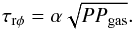 (12)This prescription was introduced by Taam & Lin (1984) in the context of the Rapid Burster and used later by Done & Davis (2008) and Czerny et al. (2009) both for galactic sources and AGNs.
In the current work, we apply a more general approach and introduce the entire family of models, with the contribution of the radiation pressure to the stress tensor parameterised by a power-law relation with an index μ ∈ [ 0,1 ]. We therefore construct a continuous transition between the disk, which is totally gas pressure dominated, and the radiation pressure that influences the heat production (Szuszkiewicz 1990; Honma et al. 1991; Watarai & Mineshige 2003; Merloni & Nayakshin 2006). The formula for the stress tensor is a generalisation of the formulae in Eqs. ()−() and is given by: 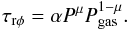 (13)In this work, we investigate the behaviour of the accretion disk described by formula (13) for a very broad range of black holes and different values of μ. A similar analysis has been performed also by Merloni & Nayakshin (2006) for different values of α (here, we fix our α with a constant value, which is at the level of 0.02). Regarding the existence of a magnetic field inside the accretion disk, the viscosity can be magnetic in origin, and can reach different values for differently magnetised disks. As the strong global magnetic field can stabilise the disk (Czerny et al. 2003; Sa¸dowski 2016), the parameter μ can be treated as an effective prescription of magnetic field.
2.4. Numerics
We use the code GLADIS (GLobal Accretion Disk InStability), whose basic framework was initially described by Janiuk et al. (2002). The code was subsequently developed and applied in a number of works to model the evolution of accretion disks in Galactic X-ray binaries and AGNs (Janiuk & Czerny 2005; Czerny et al. 2009; Janiuk & Misra 2012). The code allows for computations with a variable time-step down to a thermal timescale, adjusting to the speed of local changes of the disk structure. Our method was recently used for modelling the behaviour of the microquasar IGR J17091 (Janiuk et al. 2015). In that work, we used the prescription for a radiation-pressure dominated disk (with μ = 1, explicitly), but with an explicit formula approximating wind outflow, which regulates the amplitudes of the flares, or even temporarily leads to a completely stable disk. Here, we modified the methodology, and added the parameter μ, which allows for a continuous transition between the gas and radiation pressure dominated cases, for example, with μ ∈ [ 0,1 ], as described by Eq. (13). We neglect the wind outflow, though, as in many sources the observable constraints for its presence are too weak.
2.5. Parameters and characteristics of the results
We start time-dependent computations from a certain initial state. This evolves for some time until the disk develops a specific regular behaviour pattern. We can get either a constant luminosity of the disk (i.e. stable solution), flickering, or periodic lightcurves, depending on the model parameters. We parameterise the models by the global parameters: the black hole mass M, the external accretion rate, as well as the physical prescription for the stress, α and μ. In this study we mostly limited our modelling to a constant (arbitrary) value of α = 0.02, since the scaling with α is relatively simple, and we wanted to avoid computing the four-dimensional grid of the models. We discuss our motivation below, and we also perform a limited analysis of the expected dependence on this parameter.
Those parameters are not directly measured for the observed sources. In the current work, we focus on the unstable accretion disks. We thus construct from our models a set of output parameters that can be relatively easily measured from the observational data: the average bolometric luminosity L, the maximum bolometric luminosity Lmax, the minimum bolometric luminosity Lmin, the relative amplitude of a flare,  , and the period, P.
In order to parameterise the shape of the light curve, we also introduce a dimensionless parameter Δ, which is equal to the radio of the flare duration to the period. We define flare duration as the time between the moments where the luminosity is equal to (Lmax + Lmin)/2 on the ascending slope of the flare, and the luminosity (Lmax + Lmin)/2 on the descending slope of the flare. We then compare L, A, P and Δ obtained for several distinct black hole mass scales. In Table 1 we summarise the model input parameters. The accretion rate ṁ is presented in Eddington units  . The Eddington accretion rate ṀEdd is proportional to the Eddington luminosity, and inversely proportional to the accretion efficiency
  . In this work, we focus on the case of an accretion disk around a Schwarzschild BH with radius
  . We assume accretion efficiency
  for all models in this paper.
In Table 2 we summarise the probed characteristics of the resulting flares.
Summary of the model input parameters.
Summary of the characteristic quantities used to describe the accretion disk flares.
2.5.1. Value of α viscosity parameter
Our choice of α = 0.02 as a reference value was motivated by observations of AGNs. Siemiginowska & Czerny (1989) interpreted the quasar variability as the local thermal timescale at a radius corresponding to the observed wavelength in the accretion disk, and they determined the value of 0.1 for a small sample of quasars. The same method, for larger sample objects (Palomar-Green quasar sample), gave the constraints 0.01 <α< 0.03 for sources with luminosities 0.01LEdd<L<LEdd (Starling et al. 2004). Values in the range 0.104 <α< 0.337 were found for blazars from their intra-day variability (Xie et al. 2009) but those variations, even if related to the accretion disk, might be coming from Doppler-boosted emission and the timescale is then under-estimated.
The stochastic model of AGN variability (Kelly et al. 2009; Kozłowski 2016) allows for determination of the characteristic timescales and their scaling. Kelly et al. (2009) give the value of the viscosity parameter α = 10-3 estimated at the distance of 100 RSchw, but the actual value implied by Eq. (5)in Kelly et al. (2009) is 0.2. This value would be lower if the radius was smaller. More precise results come from Kozłowski (2016). From this paper we have ![Mathematical equation: \begin{equation} \tau_{\rm char} [{\rm years}] = 0.97 \Bigg[ \frac{M}{8 \times 10^8~M_{\odot}} \Bigg] ^{0.38\, \pm\, 0.15}\cdot \end{equation}](/articles/aa/full_html/2017/07/aa29672-16/aa29672-16-eq75.png) (14)This characteristic timescale is obtained at a fixed wavelength band, or disk temperature, and the location of a fixed disk temperature T in the Shakura-Sunyaev disk also depends on the black hole mass. We thus identify this timescale with the thermal timescale, and obtain an expression for the viscosity parameter
(14)This characteristic timescale is obtained at a fixed wavelength band, or disk temperature, and the location of a fixed disk temperature T in the Shakura-Sunyaev disk also depends on the black hole mass. We thus identify this timescale with the thermal timescale, and obtain an expression for the viscosity parameter ![Mathematical equation: \begin{equation} \alpha = 0.4 \left(\frac{T}{10^{4} {\rm K}}\right)^{-2} \left[ \frac{M}{8 \times 10^8~M_{\odot}} \right] ^{0.12\, \pm\, 0.15}\cdot \end{equation}](/articles/aa/full_html/2017/07/aa29672-16/aa29672-16-eq77.png) (15)We see that the viscosity does not depend on the black hole mass within the error. The variability study of (Kozłowski 2016) was perfomed predominantly in the r SDSS band (6231 Å), quasars being mostly at redshift 2. The conversion between the local disk temperature and the maximum disk contribution at a given wavelength is given approximately as hν = 2.43kT (where h and k are the Planck and Boltzmann constants). Therefore the dominant temperature in the Kozłowski (2016) sample is about 28 000 K, and the corresponding viscosity parameter is 0.044 for the black hole mass ~ 8.0 × 10⁸M⊙ and 0.015 for ~ 8.0 × 10⁴M⊙.
(15)We see that the viscosity does not depend on the black hole mass within the error. The variability study of (Kozłowski 2016) was perfomed predominantly in the r SDSS band (6231 Å), quasars being mostly at redshift 2. The conversion between the local disk temperature and the maximum disk contribution at a given wavelength is given approximately as hν = 2.43kT (where h and k are the Planck and Boltzmann constants). Therefore the dominant temperature in the Kozłowski (2016) sample is about 28 000 K, and the corresponding viscosity parameter is 0.044 for the black hole mass ~ 8.0 × 10⁸M⊙ and 0.015 for ~ 8.0 × 10⁴M⊙.
In following sections of this paper, we thus fix the parameter α = 0.02 in most of the models. For the exact determination of the HLX-1 mass we tried to slightly change this parameter. For the case of microquasars, we computed a small grid for one particular value of mass, accretion rate, and μ. We noticed the power dependencies between the observables (P, A, Δ) and the value of α. These functions are described in Sect. 8.1.
3. Local stability analysis
We first perform a local stability analysis in order to formulate basic expectations and limit the parameter space. In general, the disk is locally thermally unstable if for some temperature T and radius r, the local heating rate grows with the temperature faster than the local cooling rate: 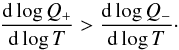 (16)In this analysis, we consider timescales that are different for the thermal and viscous phenomena which is justified for a thin disk.
3.1. Stability and timescales
For thin, opaque accretion disks, we have strong timescale separation between thermal (connected with the local heating and cooling) and viscous phenomena. The thermal timescale, for a disk rotating with angular velocity Ω, is tth = α-1Ω-1. The appearance of viscous phenomena, connected with the large-scale angular momentum transfer is connected with the disk thickness, so that  . We focus now on the thermal phenomena. On thermal timescales the local disk surface density is constant, and only the vertical inflation is allowed. Therefore, for that timescale we can assume Σ = const. From Eqs. (7) and (12) we have:
 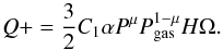 (17)Assuming that the disk maintains the vertical hydrostatic equilibrium H = P/ (C3ΣΩ2), and defining
  , we can rewrite Eq. () as:
  (18)Then, if we assume a constant Σ regime, we have:
 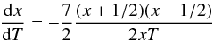 (19)and
  (20)where
 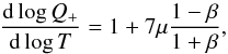 . Finally, from Eqs. (9) and (16), we have:
  (21)which is fulfilled if the condition:
  (22)is satisfied (Szuszkiewicz 1990). This gives the necessary condition for the instability for the case of μ-model, so that the instability occurs only if μ> 3/7.
3.2. Magnetised disk and its equivalence to μ model
The existence of strong magnetic fields can stabilise the radiation-pressure dominated disk (Svensson & Zdziarski 1994; Czerny et al. 2003; Sa¸dowski 2016). We can assume a significant magnetic contribution to the total pressure P, defining it as follows:  (23)Let us define the disk magnetisation coefficient
  . We put the formula () into the Shakura-Sunyaev stress-energy tensor (i.e. for μ = 0 in Eq. (18)), and then we get:
  (24)Here, the value of
  means that there is an equipartition between the energy density of the gas radiation and magnetic energy density. It corresponds to the complete stabilisation of the disk, so that
  . From the formula (22) we can connect β′ and μ as follows:
  (25)Regarding the observed features, the model of the magnetised disk is equivalent to the μ model for the radiation-pressure dominated disks in terms of appearance of thermal instability. The major difference is that the greater total pressure makes the disk thicker. This fact can have some influence on the behaviour of the light curve, which we discuss below.
3.3. Disk magnetisation and amplitude
The energy Eq. () can give us a direct connection between the heating rate and pressure. If we assume that the heating rate dominates the cooling rate, we have:  (26)where C is a constant on the thermal timescale and depends on the local values of Σ and Ω. This simple, first-order differential equation gives us the following dependence on the heating growth:
  (27)It explains why flares are sharper for bigger μ. It can also give another criterion for determination of a proper value of μ, and can be used as a test for the validity of μ-model in confrontation with the observational data. If we assume that most of the luminosity comes from a hot, thermally unstable region of the disk (Janiuk et al. 2015) and we apply it to (27), we get:
  (28)Regarding the timescale separation, and assuming that the flaring of the disk is stopped by the viscous phenomena after t ≈ tvisc, we get the following formula for the dependence between the relative amplitude and the viscous to thermal timescales rate:
 ![Mathematical equation: \begin{equation} \log A = \frac{4}{7} \frac{1}{1-\mu} \log \Bigg[ \frac{t_{\rm visc}}{t_{\rm th}} \Bigg]\cdot \end{equation}](/articles/aa/full_html/2017/07/aa29672-16/aa29672-16-eq116.png) (29)Furthermore, we can derive a useful formula that connects the presence of magnetic fields with the amplitude of the limit-cycle oscillations:
(29)Furthermore, we can derive a useful formula that connects the presence of magnetic fields with the amplitude of the limit-cycle oscillations: ![Mathematical equation: \begin{equation} \log A = \frac{1}{2} \frac{1}{ \beta'} \log \Bigg[ \frac{t_{\rm visc}}{t_{\rm th}} \Bigg]\cdot \end{equation}](/articles/aa/full_html/2017/07/aa29672-16/aa29672-16-eq117.png) (30)In the remainder of this article, we perform a more detailed analysis of the relation between the outburst amplitude and other light curve properties on the μ parameter, which is possibly corresponding to the scale of magnetic fields.
(30)In the remainder of this article, we perform a more detailed analysis of the relation between the outburst amplitude and other light curve properties on the μ parameter, which is possibly corresponding to the scale of magnetic fields.
4. Results – stationary model
First, we compute an exemplary set of stationary models, to verify the expected parameter range of the instability. Equation (22) gives the relation between the maximum gas-to-total pressure ratio and the minimum value of the μ parameter. We perform numerical computations for an intermediate black hole mass of 3 × 10⁴M⊙, and plot the stability curve at the radius  cm. The disk is locally unstable if the slope
  is negative (Eq. (16)). It gives the necessary, but not the sufficient condition for the global instability as for the appearance of the significant flares, the area of the instability should be sufficiently large. We compute the S-curves (see Sect. 1), which are presented in Fig. 1 for different values of μ. The bigger μ, the bigger the negative slope area on the S-curve, and therefore the larger the range of the instability. However, only the hot, radiation-pressure-dominated area of the disk remains unstable, and for larger radii the S-curve bend moves towards the enormously large, super-Eddingtonian external accretion rate. In effect, for sufficiently large radii, the disk remains stable. The same trend is valid also for stellar mass (microquasars) and supermassive (AGN) black holes (Janiuk & Czerny 2011).
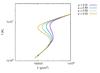 |
Fig. 1 Local stability curves for μ = 0.51, μ = 0.55, μ = 0.59 and μ = 0.63. Parameters: M = 3 × 10⁴M⊙, α = 0.02, and ṁ = 0.7. The chosen radius is |

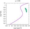 |
Fig. 2 T and Σ variability for the model with μ = 0.5 for a typical IMBH accretion disk. The computation shows a weakly developed instability. Parameters: M = 3 × 10⁴M⊙, α = 0.02, and ṁ = 0.25. The plot is made for the radius |
5. Results – time dependent model
In this section, we focus on the numerical computations of the full time-dependent model. We perform the full computations of the radiation pressure instability models since the stability curves give us only the information about the local disk stability. However, the viscous transport (Eq. (2)) and the radial temperature gradients deform the local disk structure, and the time evolution of the disk at a fixed radius resulting from the global simulations does not necessarily follow the expectations based on local stability analysis.
Figures 2 and 3 present the stability curves (red) and the global solutions of the dynamical model plotted at the same single radius (green). Stronger bending of the shape of the light curves appears for larger μ (Figs. 1–3) resulting in broader development of the instability, visible in the shape of light curves (Figs. 4, 5). Low values of μ cause the presence of the instability within a small range of radii, therefore the instability is additionally dumped by the stable zones. The time-dependent solution never sets on the stability curve, the covered area in Fig. 2 is very small, and the corresponding global light curve shows only small flickering. The growth of the instability for large values of μ results in the dynamical values of T forming two coherent sets (see Fig. 3), and the solution follows the lower branch of the stability curve. This part of the evolution describes the prolonged period between the outbursts.
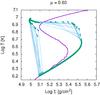 |
Fig. 3 T and Σ variability for the model with μ = 0.6 for a typical IMBH accretion disk. The models present a strongly developed instability, leading to huge outbursts. Parameters: M = 3 × 10⁴M⊙, α = 0.02, and ṁ = 0.25 for the radius |
For comparison with the observed data we need to know the global time behaviour of the disk for a broad parameter range. We ran a grid of models for typical stellar mass M = 10 M⊙, for intermediate black hole mass M = 3 × 10⁴M⊙, and for supermassive black holes (M = 108M⊙). We adopted α = 0.02 throughout all the computations, and accretion rates ranged between 10-1.6 and 10-0.2 in Eddington units. For each mass, we present the relations between period, amplitude, and duration divided by period. According to Czerny et al. (2009), the threshold accretion rate is (the sufficient rate for the flares to appear) is at the level of 0.025 for AGNs. For our models, the critical value of accretion rate is at the level of 0.025−0.1 of the Eddington rate. Below, we present our results through a set of mutual correlations between observable characteristics of the flares, P, A, and Δ (see Table 1), and the model parameters, ṁ, M, and μ.
5.1. Light curve shapes
Here we define different characteristic modes of the flares. Since we have a dynamical system described by a set of non-linear partial differential equations, we expect that the flares will form different patterns of variability, which should be comparable to the observed patterns. For that non-linear system we can distinguish between the flickering behaviour and the strong flares. In Figs. 4 and 5, we present typical cases of flickering and outburst flares. The difference between the flickering and outburst modes lies not only in their amplitudes; as we can see in Fig. 5, the long low luminosity phase, when the inner disk area remains cool, is not present in the flickering case, presented in Fig. 4. The latter, corresponds to the temperature and density variations presented in Fig. 2, where the surface density of the disk does not change significantly. In contrast, Fig. 5 presents the case where the surface density changes significantly and Σ needs a long time to grow to the value where rapid heating is possible. In the case of flickering we can distinguish two phases of the cycle: (i) heating, when the temperature in the inner regions of the disk is growing rapidly, and (ii) advective, when the inner annuli cool down significantly, and are then extinguished when the disk is sufficiently cool. Now, after a strong decrease of advection, the heating phase repeats again. In the case of the burst, the phases (i) and (ii) are much more developed and advection is able to achieve instantaneous thermal equilibrium of the disk, in contradiction to flickering, where the disk is always unstable. The instantaneous equilibrium leads to the third phase (iii), diffusive, when the surface density in the inner annuli of the disk is growing up to the moment when the stability curve has a negative slope, and the cooling rate, Q−, is significantly smaller in comparison to the heating rate, Q+. Then, the phase of heating repeats.
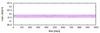 |
Fig. 4 Typical flickering light curve for intermediate mass black hole and smaller μ (M = 3 × 10⁴, μ = 0.5ṁ = 0.25). |
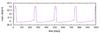 |
Fig. 5 Typical outburst light curve for intermediate mass black hole and larger μ (M = 3 × 10⁴, μ = 0.6ṁ = 0.25). |
5.2. Amplitude maps
Figure 6 shows dependencies between the accretion rate, μ coefficient, and flare amplitude. The black area corresponds to cases of stable solutions without periodic flares. The violet area corresponds to a small flickering, and red and yellow areas correspond to bright outbursts. Since for a given accretion rate and μ the AGN disks are much more radiation-pressure-dominated (Janiuk & Czerny 2011), the critical values of the accretion rates in Eddington units are the lowest for AGNs. Thus, the stabilising influence of a magnetic field is more pronounced for the microquasars, than for AGNs. Our results include different variability patterns. As shown in Fig. 6, for a given set of μ and accretion rate, the relative amplitude varies by many orders of magnitude (from small flares, changing the luminosity by only a few percent, up to the large outbursts with amplitudes of ~ 200 for microquasars, ~ 1000 for intermediate black holes, and ~ 2000 for AGN). The flare amplitude grows with accretion rate and with μ. To preserve the average luminosity on sub-Eddington level, also the light curve shape should change with at least one of these parameters. Let Δ be flare duration to period ratio, as defined in Sect. 1. To preserve the average luminosity L, the energy emitted during the flare plus energy emitted during quiescence (between the flares) should be lower than the energy emitted during one period. Since the radiation pressure instability reaches only the inner parts of the disk, the outer stable parts of the disk radiate during the entire cycle, maintaining the luminosity at the level of Lmin. This level can be computed from Eq. (1) since the outer border of the instability zone is known (Janiuk & Czerny 2011; Janiuk et al. 2015).
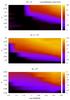 |
Fig. 6 Amplitude map for different values of accretion rates and μ for the accretion disk around a stellar-mass black hole (M = 10 M⊙, upper panel), around an intermediate-mass black hole (M = 3 × 10⁴M⊙, middle panel), and around a supermassive black hole (M = 108M⊙, lower panel). Black regions represent no flares and a lack of instability. |
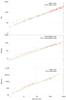 |
Fig. 7 Dependence between period and amplitude of flares for a stellar-mass black hole (M = 10 M⊙, upper panel), an intermediate-mass black hole (M = 3 × 10⁴M⊙, middle panel), and a supermassive black hole (M = 108M⊙, lower panel). Computations were made for a range of μ but values for a different μ lie predominantly along the main correlation trend resulting in a very low scatter. |
5.3. Amplitude and period
In Figure 7, we present the dependence between period and amplitude for the microquasars, intermediate mass black holes and AGN, respectively. In general, the amplitude grows with the period P, μ, and accretion rate ṁ.Figure 7 was made for the three grids of these models which result in significant limit-cycle oscillations (i.e. Lmax/Lmin> 1.2). In our work we used regular and rectangular grids. For M = 10 M⊙ and M = 3 × 10⁴M⊙ we chose α = 0.02 (as explained in Sect. 2.5.1), and the parameter ranges were μ = { 0.44,0.46,...,0.80 } and log ṁ = { −1.6,...−0.4,−0.2 }. For M = 108M⊙ we chose a different range and sampling, μ = { 0.44,0.45,...,0.56 }, but the same range of ṁ. The range of ṁ was adjusted to cover all the values for which the instability appears. The values of μ were chosen to consist of supercritical ones, according to Eq. (22) (i.e. larger than μcr = 3/7). The upper cut-off of μ (i.e. 0.8 for XRBs and IMBHs, and 0.56 for AGNs) was chosen because of computational complexity that arises for larger μ. Nevertheless, the observed properties of the sources (see, e.g. Table 5 in Sect. 8) suggest that in any case the values of μ are limited.
The results shown by points in Fig. 7 can be fitted with the following formula: ![Mathematical equation: \begin{equation} \log P ~ [{\rm s}] \approx 0.83 \log \frac{ L_{\rm max}}{ L_{\rm min}} + 1.15 \log M + 0.40. \label{eq:20160713} \end{equation}](/articles/aa/full_html/2017/07/aa29672-16/aa29672-16-eq159.png) (31)Here P is the period in seconds and M is the mass in Solar masses. The above general relation gains the following forms, if we want to use it for the sources with different black hole mass scales:
(31)Here P is the period in seconds and M is the mass in Solar masses. The above general relation gains the following forms, if we want to use it for the sources with different black hole mass scales: ![Mathematical equation: \begin{equation} \log P_{\rm MICR} ~ [{\rm s}] \approx 0.83 \log \frac{ L_{\rm max}}{ L_{\rm min}} + 1.15 \log \frac{M}{10~M_\odot} + 1.55, \end{equation}](/articles/aa/full_html/2017/07/aa29672-16/aa29672-16-eq160.png) (32)for the microquasars (see fit on Fig. 7), then
(32)for the microquasars (see fit on Fig. 7), then ![Mathematical equation: \begin{equation} \log P_{\rm IMBH} ~ [{\rm days}] \approx 0.83 \log \frac{ L_{\rm max}}{ L_{\rm min}} + 1.15 \log \frac{M}{3 \times 10^4~M_\odot} + 0.53 \label{eq:20160713i} \end{equation}](/articles/aa/full_html/2017/07/aa29672-16/aa29672-16-eq161.png) (33)for intermediate mass black holes (see fit on Fig. 7), and finally
(33)for intermediate mass black holes (see fit on Fig. 7), and finally ![Mathematical equation: \begin{eqnarray} \log P_{\rm AGN} ~ [{\rm yr}] \approx 0.83 \log \frac{ L_{\rm max}}{ L_{\rm min}} + 1.15 \log \frac{M}{10^8~M_\odot} + 2.1 \label{eq:20160713a} \end{eqnarray}](/articles/aa/full_html/2017/07/aa29672-16/aa29672-16-eq162.png) (34)for active galaxies (see fit on Fig. 7).
(34)for active galaxies (see fit on Fig. 7).
From the formula (31) we can estimate the values of masses of objects, if the values of P and A are known. The period-amplitude dependence is universal, and, in the coarse approximation, does not depend on μ. The positive correlation between period and amplitude indicates that those observables originate in one non-linear process, operating on a single timescale. Although the variability patterns can vary for different accretion rates, for a given mass, the period and amplitude are strongly correlated and can describe the range of instability development. It can, in general, be adjusted by the specific model parameters, but the basic disk variability pattern is universal in that picture.
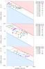 |
Fig. 8 Dependence between the amplitude and width of flares for a stellar-mass black hole (M = 10 M⊙, upper panel), an intermediate-mass black hole (M = 3 × 10⁴M⊙, middle panel), and a supermassive black hole (M = 108M⊙, lower panel). The ranges of μ are given for each figure. The colour lines represent isolines for different μ. We note that the scatter is now larger than in Fig. 7. |
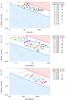 |
Fig. 9 Upper graph: dependence between period and width of flares for a stellar-mass black hole (M = 10 M⊙). The graph was prepared for a range of μ ∈ [ 0.44:0.8 ]. Middle graph: dependence between period and width of flares for an intermediate-mass black hole (M = 3 × 10⁴M⊙). The graph was prepared for a range of μ ∈ [ 0.44:0.8 ]. Lower graph: dependence between period and width of flares for a supermassive black hole (M = 108M⊙). The graph was prepared for a range of μ ∈ [ 0.44:0.56 ]. The colored lines represent isolines for different μ. |
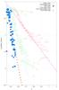 |
Fig. 10 Dependence between width, μ parameter and mass. One triangle represents one model. Triangles represent the model for the stellar-mass black hole accretion disks (M = 10 M⊙), squares represent the model for the intermediate mass black hole accretion disks (M = 3 × 10⁴M⊙) and diamonds represent the model for the supermassive black hole accretion disks (M = 3 × 10⁸M⊙). Lines represent fits for each mass. |
5.4. Amplitude and width
In Fig. 8 the relation between the flare amplitude and its width is presented. Both values are dimensionless and show similar reciprocal behaviour for the black hole accretion disks flares across many orders of magnitude. The value of Δ can help us to distinguish between different states of the source. It should be also noted that Δ depends on the amplitude of the outburst only for small amplitudes, while for the larger ones, Δ remains approximately constant. The most convenient classification is to introduce the “flickering” mode (A< 50), which corresponds to the large ratio of the flare duration to its period (Δ > 0.15), and the “outburst” mode (A> 50), which corresponds to the small flare duration to period ratio (Δ < 0.15), The latter appears for high μ and ṁ, while the former occurs for low μ and ṁ.
5.5. Width, period, and μ
In Fig. 9 the relation between the period of flares and width of flares is presented. The timescale of flare scales is approximately inversely proportional to the mass. According to Fig. 9, the flare duration to period rate Δ only weakly depends on the value of accretion rate. The dependence on μ is more significant for all the probed masses. Thus, the flare shape is determined mostly by the microphysics of the turbulent flow and its magnetisation, which is hidden in the μ parameter, and not by the amount of inflowing matter expressed by the value of accretion rate ṁ. In Fig. 10, we present the result from Fig. 9 with linear log fits connecting the values of Δ, μ, and the black hole mass M, which can be described by the formula:  (35)From Eq. (35), we can conclude that the flare shape depends predominantly on the disk magnetisation.We note that Eq. (35) enables us to estimate the behaviour of the sources even for the values of μ higher than those used in Fig. 7.As a result, for larger μ we get in general narrower flares. This effect is even more pronounced for larger black hole masses. Therefore, the outburst flares are more likely to occur for larger values of μ.
5.6. Amplitude and accretion rate
In Fig. 11 we show the dependence between relative amplitudes and accretion rates ṁ for the stellar mass, intermediate mass, and supermassive black holes, respectively. We see a monotonic dependence for any value of μ and mass. Because of the nonlinearity of evolution equations with respect to ṁ, we cannot present any simple scaling relation between ṁ and amplitudes nor periods.
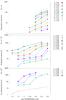 |
Fig. 11 Upper graph: dependence between amplitude and accretion rate for a stellar-mass black hole (M = 10 M⊙). Middle graph: dependence between amplitude and accretion rate for an intermediate-mass black hole (M = 3 × 10⁴M⊙). Lower graph: dependence between amplitude and accretion rate for stellar-mass black hole (M = 108M⊙). The graph was prepared for a range of μ. We can see simple unambiguous dependence for different μ-models. |
5.7. Limitations for the outburst amplitudes and periods
In Figs. 8 and 9 the dark areas mark our numerical estimations for the possibly forbidden zones in the case of microquasar accretion disks. From those figures, we get the following fitting formulae: ![Mathematical equation: \begin{eqnarray} && 0.3 \times A^{-0.5} < \Delta < 2 A^{-0.5} \label{eq:ess1} \\ && 3 \times (P~[s])^{-0.6} < \Delta < 50 \times 16 P~[s]^{-0.6}. \label{eq:ess2} \end{eqnarray}](/articles/aa/full_html/2017/07/aa29672-16/aa29672-16-eq173.png) Equations (36) and (37) result in the following estimation for P and A
Equations (36) and (37) result in the following estimation for P and A![Mathematical equation: \begin{equation} 1.96 \times A^{0.83} < P ~[s] < 630 \times A^{0.83}. \label{eq:ess3} \end{equation}](/articles/aa/full_html/2017/07/aa29672-16/aa29672-16-eq174.png) (38)In Figs. 8 and 9 we have shown the estimated range of the possibly forbidden zones in the case of the accretion disks around the intermediate-mass black holes. From those figures, we can derive the following formulae:
(38)In Figs. 8 and 9 we have shown the estimated range of the possibly forbidden zones in the case of the accretion disks around the intermediate-mass black holes. From those figures, we can derive the following formulae: ![Mathematical equation: \begin{eqnarray} && 0.07 \times A^{-0.5} < \Delta < 2.5 \times A^{-0.5} \label{eq:esi1} \\ && 0.3 (P~[{\rm days}])^{-0.6} < \Delta < 9 \times P[{\rm days}]^{-0.6}. \label{eq:esi2} \end{eqnarray}](/articles/aa/full_html/2017/07/aa29672-16/aa29672-16-eq175.png) Equations (39) and (40) result in the following estimation for P and A:
Equations (39) and (40) result in the following estimation for P and A:  (41)In Figs. 8 and 9 the dark shaded areas mark our estimations for the possibly forbidden zones for the case of supermassive black hole accretion disks. We get the following formulae from those figures:
 ![Mathematical equation: \begin{eqnarray} && 5 \times A^{-0.5} < \Delta < 70 \times A^{-0.5} \label{eq:esa1} \\ && 0.35 \times (P ~[{\rm yr}])^{-0.6} < \Delta < 2.5 \times (P ~[{\rm yr}])^{-0.6}. \label{eq:esa2} \end{eqnarray}](/articles/aa/full_html/2017/07/aa29672-16/aa29672-16-eq177.png) Equations (42) and (43) result in the following estimation for P and A:
Equations (42) and (43) result in the following estimation for P and A:  (44)
(44)
6. HLX-1 mass determination
The grids of models deliver some information about the correlation between the observed light curve features and the model parameters. From the Eq. (31) we can determine the mass of an object directly from its light curve: ![Mathematical equation: \begin{equation} M [M_\odot] = 0.45 P[s]^{0.87} A^{-0.72}. \label{eq:massestimation} \end{equation}](/articles/aa/full_html/2017/07/aa29672-16/aa29672-16-eq179.png) (45)The Δ−μ−M dependence from Fig. 10 and Eq. (35), combined with Eq. (45) gives us the exact estimation on μ
(45)The Δ−μ−M dependence from Fig. 10 and Eq. (35), combined with Eq. (45) gives us the exact estimation on μ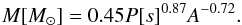 (46)The Ultraluminous X-ray sources (ULXs) are X-ray sources that exceed the Eddington limit for accretion on stellar-mass black holes (for M = 10 M⊙ the limit reaches 1.26 × 1039erg/s). It is thought that some of those objects consist of black holes with masses at the level of 100−106M⊙. Those objects are not the product of collapse of single massive stars (Davis et al. 2011). HLX-1 is the best known case of a ULX being an IMBH candidate, which has undergone six outbursts spread in time over several years with; an average period of about 400 days, a duration time of about 30−60 days, and a ratio between its maximum and minimum luminosity Lmax/Lmin of about several tens. The average bolometric luminosity ((ΣiLiΔti)/(ΣiΔti)), when Li is the luminosity at a given moment and Δti is the gap between two observation points. The SWIFT XRT observation is at the level of 1.05 × 1042 × (K/ 5) erg s-1, where K is the bolometric correction. The exact value of the bolometric correction is strongly model-dependent. The fits of the thermal state with the diskbb model (Servillat et al. 2011) imply a disk temperature Tin in the range of 0.22−0.26 keV, which, combined with the 0.2−10 keV flux and the distance to the source, implies a black hole mass of about 104, if the model is used with the appropriate normalization, and a bolometric correction of 1.5 for the 0.3−10 keV spectral range. The use of the diskbb model for larger black hole mass, 105, implies an inner temperature, Tin of 0.08 keV, much lower than observed, but then a much larger bolometric correction at 6.6. However, the larger mass cannot be ruled out on the basis of the spectral analysis since it is well known that the disk emission is much more complex than the diskbb predictions, and in particular the inner disk emission has colour temperature much higher than the local black body by a factor 2−3 (e.g. Done & Davis 2008; and see also Sutton et al. 2017). Thus the overall disk emission may not be significantly modified for the outer radii, and the hottest tail can still extend up to the soft X-ray band. A factor of 5 qualitatively accounts for that trend (Maccarone et al. 2003; Wu et al. 2016). In fact our method, which determines the mass, accretion rate, and parameters μ and α does not depend on the scaling factor connected with the bolometric luminosity and its validity is only indicative, in contradiction to P, A, and Δ estimations, that are the outcome of the non-linear internal dynamics of the accretion disk and give independent approximations on the disk parameters (e.g. see Eqs. (45) and (46)). The redshift of ESO 243-49, the host galaxy ofHLX-1, is equal to z = 0.0243, and the distance is around 95 Mpc (depending on the cosmological constants, but the uncertainty is quite small). The inclination angle is not well constrained by the observations. As we see from Eq. (44), the BH mass of HLX-1 is not sensitive to the luminosity but depends on the amplitude (A).
The observed values of the source variability period, P ≈ 400 days, and amplitude A ≈ 20 and Δ ≈ 0.13, used in the Eqs. (45) and (46), result in a black hole mass of MBH,HLX−1 ≈ 1.9 × 10⁵M⊙ and μ ≈ 0.54. These values are close to the model parameters, which are necessary to reproduce the light curve. Therefore, we conclude that our model of an accretion disk with the modified viscosity law gives a proper explanation of HLX-1 outbursts. The model to data comparison, being the result of our analysis, is presented in the Fig. 12.
The observation presented in Fig. 12 and our numerical model were presented also in Wu et al. (2016). In that article, the source HLX-1 was also compared to a broad ensemble of XRBs and AGNs. In Wu et al. (2016) we already outlined the method presented in the current work, but here we present much a more detailed description of our generalised model. In particular, we tested the large parameter space of our computations, and verified their influence on the observable characteristics of the sources. We also slightly better determined the mass of the black hole in this source. According to Eqs. (45) and (46), and Fig. 12, taking into account the value of bolometric luminosity, we propose the following parameters for HLX-1: M = 1.9 × 10⁵M⊙, ṁ = 0.09−0.18, α = 0.02 and μ = 0.54.
7. Disk flare estimations
We derive the general estimations for the oscillation period P, its amplitude A, and relative duration Δ thanks to computing a large grid of models. We achieve this despite the uncertainty of the viscosity parameter μ. The results are presented in Table 3.
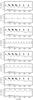 |
Fig. 12 Comparison between the SWIFT XRT observational light curve of HLX-1 and the models for different bolometric corrections K. Model parameters: μ = 0.54,α = 0.02,ṁ = 0.009 ∗ K and M = 1.9 × 10⁵M⊙. |
We compare the allowed parameters of duration to period ratios (Cols. 3 and 4), periods (Cols. 5 and 6), and flare durations (Cols. 7 and 8). We get three values of relative amplitude for each source to present possible limitations for periods and duration times. The amplitude A = 2 represents faint flares, like those in the microquasar IGR J17091 (Janiuk et al. 2015). The amplitude A = 10 corresponds to a more developed instability case, like that in the ρ states of object GRS1915 (Belloni et al. 2000). The amplitude A = 100 is connected with the huge bursts, as in HLX-1 presented in Fig. 12. The timescales presented in the Tables are on the order of minutes for the microquasars, of months for the HLXs, and of millenia for the AGN, which correspond to their viscous timescale. The period is strongly dependent on the amplitude and can change by several orders of magnitude for each mass. The estimations given here were made for the values of μ which are sufficient for the outbursts, but do not determine exactly the value of this parameter. Figure 15 (see next section) presents a universal dependence between duration times and bolometric luminosities for the X-ray sources of different scales (microquasars with M = 10 M⊙, IMBHs with M = 3 × 10⁴M⊙, and AGN with M = 108M⊙). Exact duration values from the fit presented in Eq. (51) are shown in Table 4. For microquasars, the values included in Table 3 correspond to the typical values for small and intermediate flares, the same for the case of IMBHs. In case of AGN, the appearance of big flares is necessary to verify our model with the observational data presented in the Fig. 15.
Outburst duration values for three kinds of source.
Outburst duration values for three kinds of source.
8. Summary and discussion
In this work, we studied the accretion disk instability induced by the dominant radiation pressure, with the use of the generalised prescription for the stress tensor. We adopted a power-law dependence, with an index μ, to describe the contribution of the radiation pressure to the heat production. In other words, the strength of the radiation pressure instability deepens with growing μ. We computed a large grid of time-dependent models of accretion disks, parameterised by the black hole mass, and mass accretion rate. We used the values of these parameters, which are characteristic for the microquasars, intermediate black holes, or AGN. One of our key findings is that this model can be directly applicable for determination of the black hole mass and accretion rate values, for example, for the Ultraluminous X-ray source HLX-1, and possibly also for other sources. We also found that the critical accretion rate, for which the thermal instability appears, decreases with growing μ (see Fig. 6). Also, the amplitudes of the flares of accretion disks in AGN are larger than the amplitudes of flares in microquasars and in IMBHs. The flare period grows monotonously with its amplitude, for any value of mass (see Fig. 7). The outburst width remains in a well-defined relationship with its amplitude (see Fig. 8). We also found that there is a significant negative correlation between μ and the ratio of the flare duration to the variability period, Δ. On the other hand, the dependence between the outburst amplitude A and the mass accretion rate ṁ is non-linear and complicated. Our results present different variability modes (Figs. 4 and 5). The flickering mode is presented in Fig. 4. In this mode the relative amplitude is small, and flares repeat after one another. In the burst mode the amplitude is large, and the maximum luminosity can be hundreds of times greater than minimal. An exemplary light curve is shown in Fig. 5. In this mode we observe long separation between the flares (i.e. an extended low luminosity state), dominated by the diffusive phenomena. A slow rise of the luminosity is the characteristic property of the disk instability model.
Characteristic quantities of the RXTE PCA light curves for Galactic sources presented in Altamirano et al. (2011b; Cols. 4−6) supplemented with HLX and AGNs, and estimations of the mass−α relations and magnetisation of sources (Cols. 7,8).
8.1. Mass – α relation
Since the thermal and viscous timescales strongly depend on α, which has only ad-hoc character (King 2012) and does not constitute any fundamental physical quantity, α is the parameter describing development of the MHD turbulence in the accretion disk. Thus α should, to some extent, vary depending on the source source and its state; for example, the value of α for the AGN accretion disks can differ from its value for the disks in X-ray binaries. In Fig. 13 we present different light curve shapes for six different values of α. In Fig. 14 we present the dependence of the light curve observables on α.
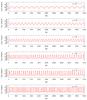 |
Fig. 13 Light curves for six different values of α for M = 10 M⊙, ṁ = 0.64, and μ = 0.6. |
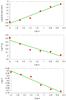 |
Fig. 14 Dependence between the α parameter and observables for M = 10 M⊙, ṁ = 0.64, and μ = 0.6 for α ∈ [ 0.01:0.32 ]. |
The formulae describing fits in Fig. 14 are as follows:  (47)where OX = A, P [in s], or Δ. The coefficients are as follows bA = 2.25 ± 0.11, cA = 0.85 ± 0.05, bP = −0.3 ± 0.05, cP = 1.85 ± 0.07, bΔ = −0.29 ± 0.03, cΔ = −0.87 ± 0.05. According to Eqs. () and () we obtain from Eq. () the following:
 ![Mathematical equation: \begin{eqnarray} && M [M_\odot] = 0.45 P[s]^{0.87} A^{-0.72} \left(\frac{\alpha}{0.02}\right)^{1.88}, \label{eq:mea} \\ && \mu = 3/7 + \frac{- \log \Delta + 0.87 \log (\frac{\alpha}{0.02})}{1.49 + 1.04 \log P - 0.864 \log A}\cdot \label{eq:muea} \end{eqnarray}](/articles/aa/full_html/2017/07/aa29672-16/aa29672-16-eq295.png)
8.2. Radiation pressure instability in microquasars
Quantitatively, our numerical computations, as well as the fitting formula (31), give the adequate description of the characteristic “heartbeat” oscillations of the two known microquasars: GRS 1915+105, and IGR 17091-324. Their profiles resemble those observed in the so-called ρ state of these sources, as found, for example, on 27th May, 1997 (Pahari et al. 2014).
For the microquasar IGR J17091, the period of the observed variability is less than 50s, as observed in the most regular heartbeat cases, that is, in the ρ and ν states (Altamirano et al. 2011a). The ν class is the second most regular variability class after ρ, much more regular than any of the other ten classes described in Belloni et al. (2000) (α, β, γ, δ, θ, κ, λ, μ, φ, χ).
The ρ state is sometimes described as “extremely regular” (Belloni et al. 2000), with a period of about 60−120 s for the case of GRS1915. The class ν includes typical Quasi-Periodic Oscillations with relative amplitude large than 2 and a period of 10−100 s.
We apply the results of the current work to model the heartbeat states qualitatively.
Equations (31) and (35) allow us to determine the values of BH masses for the accretion disks and the μ parameter. The results are given in Table 5. For the ρ-type light curves we can estimate the mass−α parameter of IGR J17091-3624 at the level of 3.2−3.5 and GRS 1915+105 at the level of 3.7−3.9. μ = 0.58−0.63 for the IGR J17091-3624 and 0.58−0.66 for the GRS1915, respectively. From the ν-type light curves we get significantly larger values of M−α parameters and μs.
Our model thus works properly for the periodic and regular oscillations, which are produced in the accretion disk for a broad range of parameters, if only the instability appears. Irregular variability states α, β, λ and μ should be regarded as results of other physical processes. The explanation of class κ of the microquasar GRS 1915 variable state, (Belloni et al. 2000) which presents modulated QPOs, seems to be on the border of applicability. In general, the method is correct for estimation of the order of magnitude, although not perfect for exact determination of the parameters due to the nonlinearity of the model. For this paper we assumed a constant value of α = 0.02 which could not be true for all values of masses. For a source with known mass, such as GRS1915 (Greiner et al. 2001; Steeghs et al. 2013), we can use previous estimations as a limitation for the value of α, as presented in Sect. 6. Steeghs et al. (2013) estimated the mass of GRS1915 at the level 10.1 ± 0.6 M⊙. From the high-frequency QPO comparison method used by Rebusco et al. (2012) we know the GRS/IGR mass ratio, which is at the level of 2.4. Combining the results of Rebusco et al. (2012) and later the GRS1915 mass estimation from Steeghs et al. (2013), for the IGRJ17091 we get M = 4.2 ± 0.25 M⊙. Results of Iyer et al. (2015) suggest the probable mass range of IGRJ17091 is between 8.7 and 15.6 M⊙.
Determination of α values based on the known IGR and GRS mass values (Rebusco et al. 2012; Steeghs et al. 2013; Iyer et al. 2015) and mass-α relation presented in Table 5.
From Tables 5 and 6 we conclude the possible dependence between α and the variability state or the source type. For the ν state of IGR we found α ≈ 0.0155−0.0165, for the ρ state of this source α ≈ 0.021−0.024, for the ν state of GRS α ≈ 0.021−0.023 and for the ρ state of GRS α ≈ 0.032−0.035. Those values can change if we assume the BHs spin, which can be near to extreme in the case of GRS1915 (Done et al. 2004) and very low, even retrograde in the case of IGR J17091 (Rao & Vadawale 2012). In our current model we neglect the presence of the accretion disk corona. If we follow the mass estimation done by Iyer et al. (2015), we get quite a consistent model for both microquasars’ ν and ρ variability states – α ≈ 0.023 for the ν state and α ≈ 0.033 the ρ state, if only we assume the mass of IGR at the level of 9−10 M⊙, that is, close to the lower limit from results of Iyer et al. (2015).
We get the above results under the assumption of negligible influence of coronal emission on the light curve. According to Merloni & Nayakshin (2006), power fraction f emitted by the corona is given by following formula: ![Mathematical equation: \begin{equation} f = \sqrt{\alpha} \Bigg[ \frac{P}{P_{\rm gas}} \Bigg]^{1 - \mu}\cdot \end{equation}](/articles/aa/full_html/2017/07/aa29672-16/aa29672-16-eq340.png) (50)For our model with α = 0.02, the values of f are low, where
(50)For our model with α = 0.02, the values of f are low, where  , which for the values of μ investigated in the paper fulfills the inequality of 0.0125 <f< 0.141, if we assume a threshold maximal value of the gas-to-total pressure rate
  from Eq. (22). According to the fact that the (heartbeat) states are strongly radiation-pressure dominated and the coronal emission rate is lower for lower values of the μ parameter, (which are more likely to reproduce the observational data), we can regard the coronal emission as negligible.
8.3. Disk instability in supermassive black holes
In the scenario of radiation pressure instability, with a considerable supply of accreting matter, the outbursts should repeat regularly every 104−106 yr (Czerny et al. 2009). From the grid of models performed in (Czerny et al. 2009), done for μ = 0.5 ( ) and 107M⊙<M< 3 × 10⁹, they obtained the following formula expressing correlation between the duration time, α parameter and bolometric luminosity Lbol:
 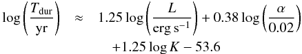 (51)which, for the special case α = 0.02 and neglecting the bolometric correction, has the following form:
  (52)The formula () also found its confirmation in observational data for different scales of BH masses, as presented in Fig. 15. This applies despite the assumption of μ = 0.5 since the expected dependence on μ is weak. If we combine Eqs. (31) and (35), we get:
  (53)From Fig. 15 we can suggest the approximate dependence
  (54)since for the same model input parameters (e.g. log ṁ = −0.2, α = 0.02 and μ = 0.56) the amplitude could be even a hundred times larger for the case of AGNs than for microquasars. Combining Eqs. (53) and (54) and adopting Lbol = ṁLEdd, ⊙ where LEdd, ⊙ = 1.26 × 1038erg s-1, we get:
  (55)The Eq. (55) can be inverted:
  (56)The above equation is a generalised version of the results from Czerny et al. (2009) and Wu et al. (2016).
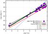 |
Fig. 15 Correlation between the bolometric luminosity and the outburst duration for different-scale BHs. Thick lines represent the best fit from Wu et al. (2016), and the prediction from Czerny et al. (2009). Thin lines represent Eq. (56) for several different values of μ, assuming ṁ = 0.1. |
In Fig. 15 we present the observational points from Wu et al. (2016), and the theoretical lines as a result from Eq. (56) for several values of μ. We assumed that the Eddington accretion rate and the accretion efficiency are roughly independent for different BH masses. The proportionality coefficient in Eq. (51) changes from 1.25 to 1.91−1.2μ, that is, 1.19 for μ = 0.6. For most of the known AGNs, except for the Low Luminosity AGNs, their luminosity in Eddington units is over 0.02 (McHardy et al. 2006), and the sources remain in their soft state, so the radiation pressure instability model should apply. The weak sources claimed to be AGNs, such as NGC 4395 and NGC 4258 (Lasota et al. 1996; Filippenko & Ho 2003) are claimed to be in the hard state, being not described accurately by the accretion disk model of Shakura-Sunyaev.
It should be possible to study the evolution of those sources statistically. Based on the known masses, accretion rates, and timescales for AGN, the luminosity distribution for the samples of AGN with similar masses or accretion rates can be acquired. This should allow us to reproduce an average light curve for a range of masses and accretion rates for a survey of the known AGNs (Wu 2009). The averaged light curve for a big ensemble of AGN will help us to provide expected luminosity distributions or luminosity-mass, luminosity-duration relations for the AGNs existing in the universe. However, high-amplitude outbursts may complicate the study since the detection of the sources between the flares may be strongly biased as the sources become very dim. Existence of the likely value of μ ≈ 0.6, proven by comparison of Eqs. (51) and (55), could also help in mass determination of newly discovered objects.
Another interesting situation comprises the so-called Changing-Look-AGN, such as IC 751 (Ricci et al. 2016). Although most AGN have a variability timescale on the order of thousands of years, the shape of model light curves (sharp and rapid luminosity increases) could suggest that, for some cases, luminosity changes can be observed.
8.4. Explanation of the HLX-1 light curve irregularity
The light curve of HLX-1, presented in the upper panel of Fig. 12, despite very regular values of peak luminosity ( between 42.5 and 42.6), presents significant variability of the flare duration. According to our model, for any constant input parameter (mass, Eddington rate, α and μ), period, duration, and amplitude should remain constant. To our knowledge, the only explanation for such a phenomenon is variation in the input parameters. The variability of the central object mass is too faint (approx. 10-8 per one cycle for any accreting source) to be visible. The variability of ṁ is possible, bearing in mind the fact that accretion rate of HLX-1 (order of 10-3M⊙ per one duty cycle) can be significantly disturbed by the tidal disruption of the minor bodies such as planets with mass ranging from 10-6M⊙ to 10-3M⊙. A detailed description of this process can be found in Evans & Kochanek (1989) and Del Santo et al. (2014) presented its application for the case of phenomena inside the globular clusters. The Eddingtion rate ṁ is a global parameter, strongly connected with the accretion disk neighbourhood (ṁ can change rapidly in the case of tidal disruption). In contradiction, μ and α are the local parameters approaching the MHD turbulence. As α can be connected with the rate of the typical velocity of turbulent movement to the sound speed (Shakura & Sunyaev 1973), μ can represent the magnetisation of the disk, as shown by the Eq. (25). In the HLX-1 observation, out of the four observables, only the Δ parameter was changing significantly between different flares. According to Eq. () this follows from changing μ. Specifically, the growth of μ from 0.48 to 0.56 is responsible for Δ decreasing from 0.4 to 0.1. According to those results, μ was growing during the sampling time, which can be explained by a decrease in disk magnetisation.
8.5. Conclusions
We propose a possible application of the modified viscosity model as a description of a regular variability pattern (heartbeat states) of black hole accretion disks for the microquasars, IMBHs and AGNs. The model works for optically thick, geometrically thin disks and determines the range and scale of the radiation pressure instability. The parameter μ, which describes viscosity, can reproduce a possibly stabilising influence of the strong magnetic field in the accretion disk. Nonlinearity of the models causes appearance of different modes of the disk state (stable disk, flickering, outbursts). Thanks to the computation of computing a large grid of models we are able to present quantitative estimations for the variability periods and amplitudes, and our model light curves reproduce several different variability patterns. Also, many observables, such as, L, P, A, and Δ, can be used directly to determine the physical parameters, like α, μ, M, and ṁ. Finally, our model can be successfully applied to the mass and accretion rate determination for the intermediate black hole HLX-1 at the level of 1.9 × 10⁵M⊙ and 0.09−0.18 respectively, updating the result from Wu et al. (2016). The prospects of further applications to microquasars and AGNs are promising.
Acknowledgments
We thank Petra Sukova for helpful discussions, Conor Wildy for the language corrections and the anonymous referee for constructive comments. This work was supported in part by the grants DEC-2012/05/E/ST9/03914 and 2015/18/M/ST9/00541 from the Polish National Science Center.
References
- Abramowicz, M. A., Czerny, B., Lasota, J. P., & Szuszkiewicz, E. 1988, ApJ, 332, 646 [NASA ADS] [CrossRef] [Google Scholar]
- Altamirano, D., Belloni, T., Linares, M., et al. 2011a, ApJ, 742, L17 [NASA ADS] [CrossRef] [Google Scholar]
- Altamirano, D., Linares, M., van der Klis, M., et al. 2011b, ATel, 3225, 1 [NASA ADS] [Google Scholar]
- Belloni, T., Klein-Wolt, M., Méndez, M., van der Klis, M., & van Paradijs, J. 2000, A&A, 355, 271 [NASA ADS] [Google Scholar]
- Brandt, W. N., Mathur, S., & Elvis, M. 1997, MNRAS, 285, L25 [NASA ADS] [CrossRef] [Google Scholar]
- Capitanio, F., Giroletti, M., Molina, M., et al. 2009, ApJ, 690, 1621 [NASA ADS] [CrossRef] [Google Scholar]
- Capitanio, F., Del Santo, M., Bozzo, E., et al. 2012, MNRAS, 422, 3130 [NASA ADS] [CrossRef] [Google Scholar]
- Czerny, B., Nikołajuk, M., Różańska, A., et al. 2003, A&A, 412, 317 [NASA ADS] [CrossRef] [EDP Sciences] [Google Scholar]
- Czerny, B., Siemiginowska, A., Janiuk, A., Nikiel-Wroczyński, B., & Stawarz, Ł. 2009, ApJ, 698, 840 [NASA ADS] [CrossRef] [Google Scholar]
- Davis, S. W., Narayan, R., Zhu, Y., et al. 2011, ApJ, 734, 111 [NASA ADS] [CrossRef] [Google Scholar]
- Del Santo, M., Nucita, A. A., Lodato, G., et al. 2014, MNRAS, 444, 93 [NASA ADS] [CrossRef] [Google Scholar]
- Done, C., & Davis, S. W. 2008, ApJ, 683, 389 [NASA ADS] [CrossRef] [Google Scholar]
- Done, C., Wardziński, G., & Gierliński, M. 2004, MNRAS, 349, 393 [NASA ADS] [CrossRef] [Google Scholar]
- Evans, C. R., & Kochanek, C. S. 1989, ApJ, 346, L13 [NASA ADS] [CrossRef] [Google Scholar]
- Farrell, S. A., Webb, N. A., Barret, D., Godet, O., & Rodrigues, J. M. 2009, Nature, 460, 73 [NASA ADS] [CrossRef] [PubMed] [Google Scholar]
- Filippenko, A. V., & Ho, L. C. 2003, ApJ, 588, L13 [NASA ADS] [CrossRef] [Google Scholar]
- Foschini, L., Berton, M., Caccianiga, A., et al. 2015, A&A, 575, A13 [NASA ADS] [CrossRef] [EDP Sciences] [Google Scholar]
- Godet, O., Plazolles, B., Kawaguchi, T., et al. 2012, ApJ, 752, 34 [NASA ADS] [CrossRef] [Google Scholar]
- Greiner, J., Cuby, J. G., & McCaughrean, M. J. 2001, Nature, 414, 522 [NASA ADS] [CrossRef] [PubMed] [Google Scholar]
- Hirose, S., Krolik, J. H., & Stone, J. M. 2006, ApJ, 640, 901 [NASA ADS] [CrossRef] [Google Scholar]
- Honma, F., Kato, S., & Matsumoto, R. 1991, PASJ, 43, 147 [NASA ADS] [Google Scholar]
- Iyer, N., Nandi, A., & Mandal, S. 2015, ApJ, 807, 108 [NASA ADS] [CrossRef] [Google Scholar]
- Janiuk, A., & Czerny, B. 2005, MNRAS, 356, 205 [NASA ADS] [CrossRef] [Google Scholar]
- Janiuk, A., & Czerny, B. 2011, MNRAS, 414, 2186 [Google Scholar]
- Janiuk, A., & Misra, R. 2012, A&A, 540, A114 [NASA ADS] [CrossRef] [EDP Sciences] [Google Scholar]
- Janiuk, A., Czerny, B., & Siemiginowska, A. 2002, ApJ, 576, 908 [NASA ADS] [CrossRef] [Google Scholar]
- Janiuk, A., Grzedzielski, M., Capitanio, F., & Bianchi, S. 2015, A&A, 574, A92 [NASA ADS] [CrossRef] [EDP Sciences] [Google Scholar]
- Jiang, Y.-F., Stone, J. M., & Davis, S. W. 2013, ApJ, 778, 65 [NASA ADS] [CrossRef] [Google Scholar]
- Kelly, B. C., Bechtold, J., & Siemiginowska, A. 2009, ApJ, 698, 895 [Google Scholar]
- King, A. 2012, Mem. Soc. Astron. Ital., 83, 466 [Google Scholar]
- Kozłowski, S. 2016, ApJ, 826, 118 [NASA ADS] [CrossRef] [Google Scholar]
- Kunert-Bajraszewska, M., & Janiuk, A. 2011, ApJ, 736, 125 [NASA ADS] [CrossRef] [Google Scholar]
- Kuulkers, E., Lutovinov, A., Parmar, A., et al. 2003, ATel, 149, 1 [NASA ADS] [Google Scholar]
- Lasota, J.-P., Abramowicz, M. A., Chen, X., et al. 1996, ApJ, 462, 142 [NASA ADS] [CrossRef] [Google Scholar]
- Lasota, J.-P., Alexander, T., Dubus, G., et al. 2011, ApJ, 735, 89 [NASA ADS] [CrossRef] [Google Scholar]
- Lightman, A. P., & Eardley, D. M. 1974, ApJ, 187, L1 [NASA ADS] [CrossRef] [Google Scholar]
- Maccarone, T. J., Gallo, E., & Fender, R. 2003, MNRAS, 345, L19 [NASA ADS] [CrossRef] [Google Scholar]
- McHardy, I. M., Koerding, E., Knigge, C., Uttley, P., & Fender, R. P. 2006, Nature, 444, 730 [NASA ADS] [CrossRef] [PubMed] [Google Scholar]
- Merloni, A., & Nayakshin, S. 2006, MNRAS, 372, 728 [NASA ADS] [CrossRef] [Google Scholar]
- Mishra, B., Fragile, P. C., Johnson, L. C., & Kluźniak, W. 2016, MNRAS, 463, 3437 [NASA ADS] [CrossRef] [Google Scholar]
- Nayakshin, S., Rappaport, S., & Melia, F. 2000, ApJ, 535, 798 [NASA ADS] [CrossRef] [Google Scholar]
- Neilsen, J., Remillard, R. A., & Lee, J. C. 2011, ApJ, 737, 69 [NASA ADS] [CrossRef] [Google Scholar]
- Pahari, M., Yadav, J. S., & Bhattacharyya, S. 2014, ApJ, 783, 141 [NASA ADS] [CrossRef] [Google Scholar]
- Peterson, B. M., McHardy, I. M., Wilkes, B. J., et al. 2000, ApJ, 542, 161 [NASA ADS] [CrossRef] [Google Scholar]
- Rao, A., & Vadawale, S. V. 2012, ApJ, 757, L12 [NASA ADS] [CrossRef] [Google Scholar]
- Rebusco, P., Moskalik, P., Kluźniak, W., & Abramowicz, M. A. 2012, A&A, 540, L4 [NASA ADS] [CrossRef] [EDP Sciences] [Google Scholar]
- Revnivtsev, M., Gilfanov, M., Churazov, E., & Sunyaev, R. 2003, ATel, 150, 1 [NASA ADS] [Google Scholar]
- Ricci, C., Bauer, F. E., Arevalo, P., et al. 2016, ApJ, 820, 5 [NASA ADS] [CrossRef] [Google Scholar]
- Sakimoto, P. J., & Coroniti, F. V. 1981, ApJ, 247, 19 [NASA ADS] [CrossRef] [Google Scholar]
- Sakimoto, P. J., & Coroniti, F. V. 1989, ApJ, 342, 49 [NASA ADS] [CrossRef] [Google Scholar]
- Sądowski, A. 2016, MNRAS, 459, 4397 [NASA ADS] [CrossRef] [Google Scholar]
- Servillat, M., Farrell, S. A., Lin, D., et al. 2011, ApJ, 743, 6 [NASA ADS] [CrossRef] [Google Scholar]
- Shakura, N. I., & Sunyaev, R. A. 1973, A&A, 24, 337 [NASA ADS] [Google Scholar]
- Siemiginowska, A., & Czerny, B. 1989, in NATO Advanced Science Institutes (ASI) Series C, 290, ed. F. Meyer, 29 [Google Scholar]
- Soria, R., Hau, G. K. T., & Pakull, M. W. 2013, ApJ, 768, L22 [NASA ADS] [CrossRef] [Google Scholar]
- Starling, R. L. C., Siemiginowska, A., Uttley, P., & Soria, R. 2004, MNRAS, 347, 67 [NASA ADS] [CrossRef] [Google Scholar]
- Steeghs, D., McClintock, J. E., Parsons, S. G., et al. 2013, ApJ, 768, 185 [NASA ADS] [CrossRef] [Google Scholar]
- Straub, O., Godet, O., Webb, N., Servillat, M., & Barret, D. 2014, A&A, 569, A116 [NASA ADS] [CrossRef] [EDP Sciences] [Google Scholar]
- Suková, P., Grzedzielski, M., & Janiuk, A. 2016, A&A, 586, A143 [NASA ADS] [CrossRef] [EDP Sciences] [Google Scholar]
- Sutton, A. D., Swartz, D. A., Roberts, T. P., et al. 2017, ApJ, 836, 48 [NASA ADS] [CrossRef] [Google Scholar]
- Svensson, R., & Zdziarski, A. A. 1994, ApJ, 436, 599 [NASA ADS] [CrossRef] [Google Scholar]
- Szuszkiewicz, E. 1990, MNRAS, 244, 377 [NASA ADS] [Google Scholar]
- Taam, R. E., & Lin, D. N. C. 1984, ApJ, 287, 761 [NASA ADS] [CrossRef] [Google Scholar]
- Taam, R. E., Chen, X., & Swank, J. H. 1997, ApJ, 485, L83 [NASA ADS] [CrossRef] [Google Scholar]
- Watarai, K.-y., & Mineshige, S. 2003, ApJ, 596, 421 [NASA ADS] [CrossRef] [Google Scholar]
- Wiersema, K., Farrell, S. A., Webb, N. A., et al. 2010, ApJ, 721, L102 [NASA ADS] [CrossRef] [Google Scholar]
- Wu, Q. 2009, MNRAS, 398, 1905 [NASA ADS] [CrossRef] [Google Scholar]
- Wu, Q., Czerny, B., Grzedzielski, M., et al. 2016, ApJ, 833, 79 [NASA ADS] [CrossRef] [Google Scholar]
- Xie, Z. H., Ma, L., Zhang, X., et al. 2009, ApJ, 707, 866 [NASA ADS] [CrossRef] [Google Scholar]
All Tables
Summary of the characteristic quantities used to describe the accretion disk flares.
Characteristic quantities of the RXTE PCA light curves for Galactic sources presented in Altamirano et al. (2011b; Cols. 4−6) supplemented with HLX and AGNs, and estimations of the mass−α relations and magnetisation of sources (Cols. 7,8).
Determination of α values based on the known IGR and GRS mass values (Rebusco et al. 2012; Steeghs et al. 2013; Iyer et al. 2015) and mass-α relation presented in Table 5.
All Figures
|
Fig. 1 Local stability curves for μ = 0.51, μ = 0.55, μ = 0.59 and μ = 0.63. Parameters: M = 3 × 10⁴M⊙, α = 0.02, and ṁ = 0.7. The chosen radius is |
| In the text | |
|
Fig. 2 T and Σ variability for the model with μ = 0.5 for a typical IMBH accretion disk. The computation shows a weakly developed instability. Parameters: M = 3 × 10⁴M⊙, α = 0.02, and ṁ = 0.25. The plot is made for the radius |
| In the text | |
|
Fig. 3 T and Σ variability for the model with μ = 0.6 for a typical IMBH accretion disk. The models present a strongly developed instability, leading to huge outbursts. Parameters: M = 3 × 10⁴M⊙, α = 0.02, and ṁ = 0.25 for the radius |
| In the text | |
|
Fig. 4 Typical flickering light curve for intermediate mass black hole and smaller μ (M = 3 × 10⁴, μ = 0.5ṁ = 0.25). |
| In the text | |
|
Fig. 5 Typical outburst light curve for intermediate mass black hole and larger μ (M = 3 × 10⁴, μ = 0.6ṁ = 0.25). |
| In the text | |
|
Fig. 6 Amplitude map for different values of accretion rates and μ for the accretion disk around a stellar-mass black hole (M = 10 M⊙, upper panel), around an intermediate-mass black hole (M = 3 × 10⁴M⊙, middle panel), and around a supermassive black hole (M = 108M⊙, lower panel). Black regions represent no flares and a lack of instability. |
| In the text | |
|
Fig. 7 Dependence between period and amplitude of flares for a stellar-mass black hole (M = 10 M⊙, upper panel), an intermediate-mass black hole (M = 3 × 10⁴M⊙, middle panel), and a supermassive black hole (M = 108M⊙, lower panel). Computations were made for a range of μ but values for a different μ lie predominantly along the main correlation trend resulting in a very low scatter. |
| In the text | |
|
Fig. 8 Dependence between the amplitude and width of flares for a stellar-mass black hole (M = 10 M⊙, upper panel), an intermediate-mass black hole (M = 3 × 10⁴M⊙, middle panel), and a supermassive black hole (M = 108M⊙, lower panel). The ranges of μ are given for each figure. The colour lines represent isolines for different μ. We note that the scatter is now larger than in Fig. 7. |
| In the text | |
|
Fig. 9 Upper graph: dependence between period and width of flares for a stellar-mass black hole (M = 10 M⊙). The graph was prepared for a range of μ ∈ [ 0.44:0.8 ]. Middle graph: dependence between period and width of flares for an intermediate-mass black hole (M = 3 × 10⁴M⊙). The graph was prepared for a range of μ ∈ [ 0.44:0.8 ]. Lower graph: dependence between period and width of flares for a supermassive black hole (M = 108M⊙). The graph was prepared for a range of μ ∈ [ 0.44:0.56 ]. The colored lines represent isolines for different μ. |
| In the text | |
|
Fig. 10 Dependence between width, μ parameter and mass. One triangle represents one model. Triangles represent the model for the stellar-mass black hole accretion disks (M = 10 M⊙), squares represent the model for the intermediate mass black hole accretion disks (M = 3 × 10⁴M⊙) and diamonds represent the model for the supermassive black hole accretion disks (M = 3 × 10⁸M⊙). Lines represent fits for each mass. |
| In the text | |
|
Fig. 11 Upper graph: dependence between amplitude and accretion rate for a stellar-mass black hole (M = 10 M⊙). Middle graph: dependence between amplitude and accretion rate for an intermediate-mass black hole (M = 3 × 10⁴M⊙). Lower graph: dependence between amplitude and accretion rate for stellar-mass black hole (M = 108M⊙). The graph was prepared for a range of μ. We can see simple unambiguous dependence for different μ-models. |
| In the text | |
|
Fig. 12 Comparison between the SWIFT XRT observational light curve of HLX-1 and the models for different bolometric corrections K. Model parameters: μ = 0.54,α = 0.02,ṁ = 0.009 ∗ K and M = 1.9 × 10⁵M⊙. |
| In the text | |
|
Fig. 13 Light curves for six different values of α for M = 10 M⊙, ṁ = 0.64, and μ = 0.6. |
| In the text | |
|
Fig. 14 Dependence between the α parameter and observables for M = 10 M⊙, ṁ = 0.64, and μ = 0.6 for α ∈ [ 0.01:0.32 ]. |
| In the text | |
|
Fig. 15 Correlation between the bolometric luminosity and the outburst duration for different-scale BHs. Thick lines represent the best fit from Wu et al. (2016), and the prediction from Czerny et al. (2009). Thin lines represent Eq. (56) for several different values of μ, assuming ṁ = 0.1. |
| In the text | |
Current usage metrics show cumulative count of Article Views (full-text article views including HTML views, PDF and ePub downloads, according to the available data) and Abstracts Views on Vision4Press platform.
Data correspond to usage on the plateform after 2015. The current usage metrics is available 48-96 hours after online publication and is updated daily on week days.
Initial download of the metrics may take a while.