| Issue |
A&A
Volume 603, July 2017
|
|
|---|---|---|
| Article Number | A59 | |
| Number of page(s) | 24 | |
| Section | Astrophysical processes | |
| DOI | https://doi.org/10.1051/0004-6361/201629660 | |
| Published online | 06 July 2017 | |
Electromagnetic cascade masquerade: a way to mimic γ-axion-like particle mixing effects in blazar spectra
1 Federal State Budget Educational Institution of Higher Education, M.V. Lomonosov Moscow State University, Skobeltsyn Institute of Nuclear Physics (SINP MSU), 1(2), Leninskie gory, GSP-1119991 Moscow, Russia
e-mail: This email address is being protected from spambots. You need JavaScript enabled to view it.
; This email address is being protected from spambots. You need JavaScript enabled to view it.
2 Federal State Budget Educational Institution of Higher Education, M.V. Lomonosov Moscow State University, Department of Physics, 1(2), Leninskie gory, GSP-1, 119991 Moscow, Russia
Received: 5 September 2016
Accepted: 13 February 2017
Abstract
Context. Most of the studies on extragalactic γ-ray propagation performed up to now only accounted for primary γ-ray absorption and adiabatic losses, known as the “absorption-only model”. However, there is growing evidence that this model is oversimplified and must be modified in some way. In particular, it was found that the intensity extrapolated from the optically-thin energy range of some blazar spectra is insufficient to explain the optically-thick part of these spectra. This effect was interpreted as an indication for γ-axion-like particle (ALP) oscillation. On the other hand, there are many hints that a secondary component from electromagnetic cascades initiated by primary γ-rays or nuclei may be observed in the spectra of some blazars.
Aims. We study the impact of electromagnetic cascades from primary γ-rays or protons on the physical interpretation of blazar spectra obtained with imaging Cherenkov telescopes.
Methods. We used the publicly-available code ELMAG to compute observable spectra of electromagnetic cascades from primary γ-rays. For the case of primary proton, we developed a simple, fast and reasonably accurate hybrid method to calculate the observable spectrum. We performed the fitting of the observed spectral energy distributions (SEDs) with various physical models: the absorption-only model, the “electromagnetic cascade model” for the case of primary γ-rays, and several versions of the hadronic cascade model for the case of primary protons. We distinguish the following species of hadronic cascade models: 1) the “basic hadronic model”, in which it is assumed that the proton beam travels undisturbed by the extragalactic magnetic field and that all observable γ-rays are produced by primary protons through photohadronic processes with subsequent development of electromagnetic cascades; 2) the “intermediate hadronic model”, which is the same as the basic hadronic model, but the primary beam is terminated at some redshift zc; and 3) the “modified hadronic model” that includes the contribution from primary, redshifted and partially-absorbed, γ-rays.
Results. Electromagnetic cascades show at least two very distinct regimes labelled by the energy of the primary γ-ray (E0): the one-generation regime for the case of E0 < 10 TeV, and the universal regime for E0 > 100 TeV and redshift to the source zs > 0.02. Spectral signatures of the observable spectrum for the case of the basic hadronic model, zs = 0.186 and low energy (E < 200 GeV), are nearly the same as for a purely electromagnetic cascade, but for E > 200 GeV the spectrum is much harder for the case of the basic hadronic model. In the framework of the intermediate hadronic model, the observable spectrum depends only slightly on the primary proton energy, but it strongly depends on zc at E > 500 GeV. As a rule, both electromagnetic and hadronic cascade models provide acceptable fits to the observed SEDs. We show that the best-fit model intensity in the multi-TeV region of the spectrum in the framework of the electromagnetic cascade model is typically greater than the one for the case of the absorption-only model. Finally, for the case of blazar 1ES 0229+200 we provide strong constraints on the intermediate hadronic model, assuming models for the blazar emission and the magnetic field around the source.
Key words: astroparticle physics / radiation mechanisms: non-thermal / methods: numerical / BL Lacertae objects: general / cosmic background radiation
© ESO, 2017
1. Introduction
The development of ground-based γ-ray astronomy with imaging Cherenkov telescopes has been very fast during the last two decades (for a review see, e.g. Hillas 2012). Indeed, only seven years after the detection of TeV photons from the active galactic nucleus (AGN) Mkn 421 in Punch et al. (1992), the first detailed study of a blazar (an AGN with the jet presumably pointed towards the observer) spectrum was performed by Aharonian et al. (1999). Almost immediately, these observations were utilized to put some constraints on the intensity of extragalactic background light (EBL; Stecker & de Jager 1993; de Jager et al. 1994 for the former observations; and in Aharonian et al. 1999 for the latter).
Indeed, primary very high energy (VHE, E> 100 GeV) γ-rays are absorbed on EBL photons by means of the γγ → e+e− process (Nikishov 1962; Gould & Shroeder 1967), and for the case of primary energy E ~ 100 TeV and higher, on the cosmic microwave background (CMB) as well (Jelley 1966). More recently, the signatures of this absorption process were observed with the Fermi LAT instrument (Ackermann et al. 2012) and the H.E.S.S. Cherenkov telescope, Abramowski et al. (2013a) with high statistical significances of ~ 6σ and 8.8σ, respectively.
However, Horns & Meyer (2012) find that the strength of absorption at high optical depth (τγγ> 2, hereafter simply τ) appears to be lower than expected. They obtain this result on a sample of blazar spectra measured with imaging Cherenkov telescopes by comparing the distributions of the flux points for the τ regions 1 <τ< 2 and τ> 2 around the intensity extrapolated from the optically-thin regime τ< 1. The statistical significance of this effect, according to Horns & Meyer (2012), is 4.2σ. Although Biteau & Williams (2015) do not confirm this result, very recently Horns (2016) again finds an indication for this anomaly with another analysis method. This sort of an anomaly, in fact, closely resembles the so-called “TeV-IR crisis” (Protheroe & Meyer 2000) that was derived from the already mentioned observations of Mkn 501 (Aharonian et al. 1999). The “TeV-IR crisis”, however, was later found to be less severe after the development of more advanced EBL models. On the contrary, the “new” anomaly of Horns & Meyer (2012) and Horns (2016) persists for most of these contemporary models of EBL intensity.
The authors of Horns & Meyer (2012) interpret their result as an indication for the existence of some non-conventional physical effect, for instance, the process of oscillations of γ-rays into axion-like particles (ALPs) and back into photons within magnetic fields on the way from the source to the observer (γ → ALP). Indeed, photons reconverted from ALPs near the observer can significantly enhance the observed intensity in the τ> 2 region. Moreover, once the anomaly is well established, it is possible to put constraints on the γ-ALP mixing parameters ma (the mass of ALP) and gaγ (the photon-ALP coupling constant). In Meyer et al. (2013) a lower limit on the gaγ was found, depending on the ma value. For any fixed ma in the range considered in Meyer et al. (2013), some values of gaγ greater than the lower limit gaγ−min(ma) could explain the observed anomaly. Together with the upper limits from the CAST experiment (Andriamonje et al. 2007), this result allows the construction of a confidence interval for gaγ.
Besides the anomaly at τ> 2, there exists another signature of γ → ALP oscillation, namely a step-like irregularity that is situated at the energy lower than the starting energy of the VHE anomaly (e.g. Sanchez-Conde et al. 2009). The drop of intensity associated with this spectral feature is usually about one third because photons, which have two polarization states, attain equipartition with ALPs, which have one polarization state. A very recent analysis of Fermi LAT data (Ajello et al. 2016) (observations of the NGC 1275 Seyfert galaxy were used), however, did not find this signature. Moreover, other bounds (Ayala et al. 2014; Abramowski et al. 2013b; Payez et al. 2015; Wouters & Brun 2013) on the parameters of γ-ALP mixing allow strong constraint of the scenario considered in Meyer et al. (2013). Therefore, the hypothesis that the VHE anomaly is explained by γ → ALP oscillation appears to be less attractive than before; one needs to search for some other physical mechanism of the anomaly.
In this respect, we note that most of extragalactic γ-ray propagation studies were performed with account of only two elementary processes: the absorption of primary photons by means of pair-production, and their adiabatic losses. This model (hereafter “the absorption-only model”) rests on the assumption that the secondary electrons and positrons (hereafter simply “electrons” unless otherwise stated) are deflected and delayed by the extragalactic magnetic field (EGMF), thus the cascade photons produced by these electrons by means of the inverse Compton (IC) scattering do not contribute to the observed spectrum.
However, the EGMF strength B in voids of the large-scale structure (LSS) may be small enough to violate this assumption. The existing constraints (Blasi et al. 1999; Pshirkov et al. 2016; Dolag et al. 2005; Neronov & Vovk 2010; Dermer et al. 2011; Taylor et al. 2011; Vovk et al. 2012; Abramowski et al. 2014; Takahashi et al. 2012, 2013) on the EGMF strength on characteristic coherence scale 1 Mpc (Akahori & Ryu 2010), some of which have been summarized such as in Fig. 4 of Dzhatdoev (2015a), do not exclude the probability that cascade emission may contribute to the observed spectrum.
The recent work Finke et al. (2015), using a more conservative method than the above-mentioned references, excludes B< 10-19 G again on characteristic coherence scale 1 Mpc with statistical significance 5σ. Arlen et al. (2014) do not find any reason to reject the null hypothesis of B = 0 at all. Tashiro & Vachaspati (2015) found B ~ 10-14G. Their study was performed using the angular correlation pattern of Fermi LAT (Atwood et al. 2009) diffuse γ-rays, however it is not clear how much this result may be affected by the existence of comparatively strong magnetic fields in galaxy clusters.
Moreover, there are some hints that the cascade component does contribute to the observed spectrum of blazars at energies E< 300 GeV. Neronov et al. (2012), using observations of Mkn 501 in a flaring state by the Fermi LAT instrument and the VERITAS Cherenkov telescope (Abdo et al. 2011) during the 2009 multiwavelength campaign, obtain the energy spectrum dN/ dE (dN is the number of photons per energy bin dE) from 300 MeV up to 5 TeV. They find that the Fermi LAT spectrum in the 10−200 GeV energy range had a power-law (dN/ dE = C·E− γ) index γ = 1.1 ± 0.2, whereas in the 300 GeV−5 TeV γ ~ 2. It is interesting that the Fermi LAT lightcurves in the 0.3−3 GeV and 3−30 GeV energy bins do not show any evidence of strong, fast variability, whereas in the 30−300 GeV energy bin the flare is readily identified on the lightcurve. Neronov et al. (2012) find that this kind of behaviour of the spectral and timing characteristics is typical for an intergalactic cascade, assuming B ~ 10-16−10-17 G on the maximum spatial scale 1 Mpc.
Another result supporting the incompleteness of the absorption-only model was also obtained with the Fermi LAT telescope. Furniss et al. (2015) find a correlation between 10−500 GeV energy fluxes of blazars that have relatively hard, γ< 3, observed spectra above 10 GeV and the fraction along the line of sight occupied by voids in the LSS. This effect may be explained by the same physical mechanism, namely the cascade emission that is likely to be angle-broadened by the EGMF at an energy below 200−300 GeV. Finally, Chen et al. (2015) find the evidence for the existence of “pair halos” (extended emission) around the positions of various blazars, again with Fermi LAT data, thus giving additional support to the hypothesis that the cascade component may contribute to the observed spectra.
These works motivated us to study how the inclusion of the cascade component into the fitting of the VHE spectra would influence the data interpretation, especially in the optically-thick, τ> 1 region. Our paper is by far not the first study of intergalactic cascade spectra; besides the already mentioned work (Neronov et al. 2012), there are many others that include more or less detailed discussions of these, such as Aharonian et al. (1999, 2002), d’Avesac et al. (2007), Murase et al. (2012), and Takami et al. (2013).
However, in a very recent conference paper, Dzhatdoev (2015b) shows that if the primary spectrum is hard enough, γ ~ 1, and the cutoff in the spectral energy distribution (SED) of the source is situated at a sufficiently high energy, Ec ≫ 1 TeV, then the intersection of a low-energy cascade component and a high-energy primary (absorbed) component forms a kind of “ankle” that to some extent may mimic the γ-ALP mixing effect mentioned above. One of the main aims of the present paper is to discuss this effect in more depth. We will see that the last model is qualitatively different from other “electromagnetic cascade models”, meaning those models that involve intergalactic cascades initiated by primary γ-rays.
There exists another class of intergalactic cascade models of blazar spectra dealing with primary protons or nuclei that initiate secondary photons by means of photopion losses and pair production with subsequent development of electromagnetic cascades (“hadronic cascade models”) (e.g. Uryson 1998; Essey & Kusenko 2010a; Essey et al. 2010b, 2011; Murase et al. 2012; Takami et al. 2013; Essey & Kusenko 2014; Zheng et al. 2016). We compare hadronic models with the electromagnetic cascade model of Dzhatdoev (2015b) to reveal their advantages and difficulties.
The paper is organized as follows. In Sect. 2 we discuss some general properties of cascades from primary photons or protons developing on EBL/CMB and give a detailed description of our calculation method for the case of primary protons. In Sect. 3 we define the sample of blazar spectra to be used in the analysis; in this paper we focus on the observations performed with Cherenkov telescopes. In Sect. 4 we present the fits to observed SEDs. Sect. 5 contains discussion and constraints on the hadronic cascade model. Finally, in Sect. 6 the conclusions to our work are drawn.
2. Electromagnetic cascades from primary γ-rays and primary nuclei
After a primary γ-ray, travelling through the Universe, is absorbed by an EBL photon, secondary electrons may upscatter CMB/EBL photons and produce the new generation of “cascade” photons by means of the IC process. If the energy of the primary photon is high enough and the source is sufficiently distant, the number of generations in this kind of a cascade may be considerably higher than unity. In this case the spectrum of the cascade takes a universal form. On the contrary, if the energy of the primary photon is sufficiently low, but still high enough to be absorbed on EBL, the cascade takes a “degenerate” form and may be well-described by a one-generation approximation (see e.g. Dermer et al. 2011). In the next subsection we discuss both regimes and the transition between them.
When the calculations presented in this section were almost finished, we noticed the insightful paper by Berezinsky & Kalashev (2016) that discusses the universal regime in depth. We will express our results in terms of their work, when applicable. All results presented in this section are calculated for the case of a cascade particle threshold of 10 GeV, unless otherwise stated, and a redshift to the source zs = 0.186. We find the latter value to be convenient because we will see that three out of six blazars studied in this paper (Sect. 3) have redshifts very close to 0.186. In the present paper we use the ROOT (Brun & Rademakers 1997) analysis framework for drawing figures and performing a part of the analysis.
2.1. Cascades from primary γ-rays
Throughout this paper we use the publicly-available code ELMAG (Kachelriess et al. 2012) version 2.02 to calculate the observable spectra of γ-rays for the case of primary photons. In what follows, when running the ELMAG code, we assume the Kneiske & Dole (2010; hereafter KD10) EBL model. The KD10 model was the first to be implemented in the ELMAG code, therefore this code is the best-tested and most reliable with this model. All calculations with ELMAG presented in this paper are full direct MC simulations (with parameter αsmp = 0).
There has been a considerable amount of discussion as to whether pair beams resulting from the development of electromagnetic cascades are subject to plasma instabilities and additional, with respect to the IC process, energy losses. The conclusions of various studies are conflicting: although Broderick et al. (2012), Schlickeiser et al. (2012), Chang et al. (2014), and Menzler & Schlickeiser (2015) find that these effects are considerable and must be accounted for, at least in the Fermi LAT region of the spectrum; whereas Miniati & Elyiv (2013), Venters & Pavlidou (2013), Sironi & Giannios (2014), and Kempf et al. (2016) argue that plasma losses are subdominant with respect to IC losses. The last work from this list (Kempf et al. 2016) runs a detailed numerical simulation and finds that the growth rate of the instability is likely not sufficient to cause an appreciable effect. Therefore, we do not include this kind of a process in our calculations.
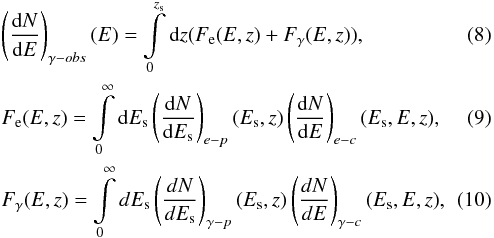
To demonstrate the basic regimes of electromagnetic cascade development on CMB/EBL, Fig. 1 presents observable spectra for different primary energies for the case of monoenergetic primary injection. Two principal components may be readily identified in Fig. 1: the cascade component itself, and the primary, absorbed, component that is seen in the right part of the graph for the case of E0 ≤ 10 TeV. The higher the energy, the more the primary component is attenuated due to a rapid rise of the τ value with increasing energy. A slight shift of the primary energy to the lower values is due to adiabatic losses. For the case of the primary energy above 10 TeV, the primary photons are almost completely absorbed due to very large value of τ for these energies.
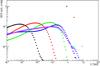 |
Fig. 1 Primary and secondary components (observable spectra) of γ-rays from primary monoenergetic injection. Black circles – primary energies E0= 1 TeV, red – 3 TeV, green – 10 TeV, blue – 30 TeV, cyan – 100 TeV, and magenta – 1000 TeV= 1 PeV. |
Figure 1 reveals two very different regimes: for the case of E0 ≤ 10 TeV the energy of the maximum in the spectral energy distribution, SED = E2dN/ dE, of the cascade component is approximately  ; whereas for the case of E0 ≥ 100 TeV the cascade spectrum is practically independent of energy. The first case may be well-described by the one-generation approximation, and the second case is essentially the universal regime. As we will see, the universality of the cascade spectrum is “weak” (Berezinsky & Kalashev 2016), meaning that the spectrum of observable γ-rays is practically independent of the energy and type, photon/electron, of the primary particle, but depends on zs. The transition between these regimes appears to be very sharp, such that the cascade completely changes its mode of propagation within only one decade of the primary energy. The physical reason for this kind of a fast transition is clear, namely the rapid rise of the γγ interaction rate in the energy range of 10−100 TeV (see, e.g. Kachelriess et al., 2012, Fig. 2 left panel). To our knowledge, no study before us has remarked upon this kind of a fast transition between these completely different regimes of cascade development.
Additional graphs of electromagnetic cascade spectra in the universal regime are presented in Appendix A. They demonstrate that the property of cascade universality is fulfilled in the observable energy range 10 GeV−30 TeV within four decades of the primary energy (from 100 TeV to 1 EeV) with an accuracy ≤30% that is independent of the primary particle type for zs ≥ 0.02.
To be able to distinquish between two categories of observable γ-rays, primary (redshifted) (type 1) and cascade (type 2) photons, we modified the output of the ELMAG code and created a database that contains an observable spectrum for every primary photon. For every array that contains an observable spectrum we performed the following classification procedure. If an array contained only one non-zero entry and the redshifted value of the primary energy fitted the energy range of the corresponding bin with the non-zero entry, the array was classified as a type 1 event. Otherwise it was classified as a type 2 event. Appendix B contains several graphs that show primary, absorbed, and cascade components for various primary spectra. These figures demonstrate that the contribution of the cascade component to the total intensity is appreciable at 100 GeV, roughly the threshold for Cherenkov telescope observations, but is only appreciable above this value if the primary spectrum is hard enough such that γ< 2 and the cutoff energy of the spectrum Ec> 10 TeV.
2.2. Cascades from primary protons
For the case of primary protons we developed an original code based on a hybrid approach. First of all, we propagated primary protons from the source to the observer, z = 0, with a small step δz = 10-5. We updated their energy at every step and computed their mean energy loss according to Berezinsky et al. (2006), Eq. (8). In this work we are interested in the case of proton energy losses on CMB. Full energy losses of a proton with energy Ep per unit time are: 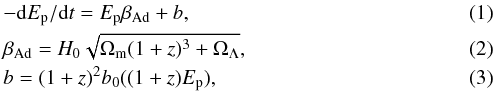 where H0 = 67.8 km s-1 Mpc-1, Ωm = 0.308 (Planck Collaboration XIII 2016), ΩΛ ≈ 1−Ωm, and b0 = −(dEp/ dt)pair + pion, representing pair production and pion production energy losses at z = 0.
The next step was the calculation of energy spectra of particles produced by primary protons. We followed Kelner & Aharonian (2008) to calculate these energy spectra. For the pair production process, the spectra of electrons (dNe/ dEe) and positrons are identical, and for the case of pair production on CMB (Kelner & Aharonian 2008, Eq. (67)):  (4)where k is the Boltzmann constant; T = (1 + z)T0 (T0 = 2.725 K is the CMB temperature at z = 0); γp = Ep/mpc2 is the proton Lorentz factor;
  , where
  is the energy of the secondary electron in the comoving frame (i.e. in the same frame where Ep is measured);
 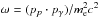 is the energy of the photon, in the rest frame of the proton, in units of electron rest energy (pp, pγ are four-momenta of the proton and photon, respectively);
  , where
  and
and 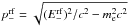 are the energy and the momentum of the electron in the rest frame of the proton, respectively; and (
 ); Σ(ω,E−,ξ) is the double-differential cross-section as a function of energy and emission angle of the electron in the rest frame of the proton (Blumenthal 1970, Eq. (10)), and (
 where the angle between the momenta of the photon and the electron is denoted as (θ−). Four examples of calculated electron SED for the case of z = 0 are shown in Fig. 2 for different values of primary proton energy Ep0. The maximum of the SED for the case of Ep0 = 100 EeV was normalized to one in this figure.
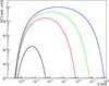 |
Fig. 2 Spectra of secondary electrons generated in the pair production process. Black line – Ep0 = 1 EeV, red – 10 EeV, green – 30 EeV, blue – 100 EeV. |
The case of photopion losses is also covered in Kelner & Aharonian (2008). We used equations from Sect. II of their work with the energy of a CMB photon ϵ = (1 + z)ϵ(z = 0) and calculated the spectra of (γ, e+, νe, νμ,  ). Because we are interested only in primary energies below 100 EeV, we neglected the flux of e− and
  . According to Kelner & Aharonian (2008), Fig. 6 (right panel), the flux of e− and contribute only about 0.1% of the total flux at Ep = 100 EeV and z = 0. We checked that both panels of Kelner & Aharonian (2008) (Fig. 6) are well-reproduced for all types of particles for which we performed our calculations. As an example of this calculation we present the SEDs of secondary γ-rays and positrons in Fig. 3 for the case of z = 0 for different values of primary proton energy. The maximum of the SED for the case of γ-rays and Ep0 = 100 EeV was normalized to 1 in this figure.
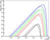 |
Fig. 3 Secondary γ (solid) and positron (dashed) SEDs for the case of photopion losses. Black lines – Ep0 = 30 EeV, red – 50 EeV, green – 70 EeV (green), blue – 100 EeV. |
We then proceeded to calculate observable, meaning cascade, γ-ray spectra. The energies of secondary γ-rays and electrons in Figs. 2 and 3 are mostly above 100 TeV, therefore the cascade universality assumption may be applied to reduce computer time requirements; this kind of a calculation is presented in the following Sect. 2.2.1. As an alternative, to validate the results obtained in the cascade universality approximation, we performed a full calculation of observable spectra without this assumption (Sect. 2.2.2). Synchrotron radiation was neglected in these calculations. In both these subsections we are interested only in the shape of the observable γ-ray spectrum. The normalization of the spectrum is discussed in Sect. 5.
2.2.1. Observable γ-ray spectra in the universal spectrum approximation
Here we assumed “weak universality”, as described above. Using the ELMAG code, we calculated an array of cascade spectra for the case of primary γ-rays with fixed energy 1 PeV but different z, which was distributed randomly and uniformly from 0 to 0.30. Although adiabatic losses do affect the energy of propagating protons, only “active”, meaning pair and photopion, losses give rise to new particles and thus eventually produce observable signal in γ-rays. The energy transferred to these particles on the step dz is: 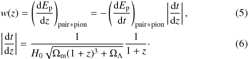 Figures 2 and 3 demonstrate that nearly all secondary particles are ultrarelativistic, and therefore nearly all the energy of these particles, except neutrinos, could be transferred to the cascade. Several examples of w(z) /w(0), meaning w(z) normalized to the value at z = 0, are shown in Fig. 4 for different values of primary proton energy. For Ep0 = 50 EeV, and especially 100 EeV, primary protons quickly lose energy near the source until they reach comparatively low energy at which the energy loss rate becomes much smaller (see Fig. 1 of Berezinsky et al. 2006). On the other hand, for the case of Ep0 = 10 EeV and 30 EeV, protons keep an appreciable fraction of their energy until they reach z = 0, and thus they keep producing secondaries very effectively, even near the observer.
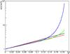 |
Fig. 4 w(z) /w(0) dependence. Black line – Ep0 = 10 EeV, red – 30 EeV, green – 50 EeV, blue – 100 EeV. |
Finally, we calculated the observable spectrum of γ-rays at z = 0. For the case of an isotropic source of primary protons: 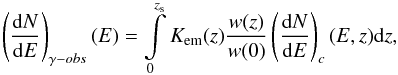 (7)where Kem(z) is the fraction of “active” losses transferred to γ-rays and electrons, and (dN/ dE)c(E,z) is the universal spectrum of the cascade with a starting point at z. Several examples of Kem(z) are shown in Fig. 5 for different values of primary proton energy. For the case of Ep0 ≤ 30 EeV, when the dominating source of proton energy loss is the pair-production process, Kem is practically equal to one.
In this paper we study the case of ultrarelativistic primary protons, Ep0> 1 EeV, and therefore, in the absence of EGMF, the angular distribution of observable γ-rays is practically coincident with the angular distribution of primary protons. Thus, Eq. (7) is justified for the conditions investigated in our work.
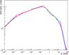 |
Fig. 6 Observable γ-ray SED. Dashed magenta line – Ethr= 10 MeV, solid cyan – 10 GeV. Black, red, green, and blue lines denote power-law approximations of the spectrum in various energy regions. |
The resulting observable SED, for the case of monoenergetic primary injection with Ep0 = 30 EeV for two options of cascade γ-ray threshold energy Ethr in ELMAG, is shown in Fig. 6. The signatures of the spectrum are highlighted with additional power-law approximations at various energy regions. The low-energy signatures of the observable spectrum, meaning the parameters of a “poly-gonato” power-law approximation at E< 200 GeV, are practically identical to the case of an electromagnetic cascade from primary γ-rays (see Berezinsky & Kalashev 2016 for a detailed discussion of this case). Indeed, for the case of our calculations, meaning primary protons, these parameters are as follows: the shape of the power-law segment is γ1 = 1.60 (for the dN/ dE spectrum) below the break at Eb1 = 230 MeV, and γ2 = 1.85 below another break at Eb2 = 200 GeV. The corresponding typical values for an electromagnetic cascade from a primary γ-ray are: γ1−EM ~ 1.5, Eb1−EM ~ 100 MeV, γ2 ~ 1.9, and Eb2−EM ~ 200−400 GeV, depending on the fitting conventions (see Fig. 3, upper panel, and Fig. 8 of Berezinsky & Kalashev 2016).
However, for higher energies, E> 200 GeV, the situation is very different. For the case of primary protons the observable spectrum is far less steep than for the case of primary γ-rays, such that γ3 = 2.40 above 200 GeV and below Eb3 = 15.2 TeV, and γ4 = 4.00 above 15.2 TeV. In this work we are interested only in E below 100 TeV; we leave the E> 100 TeV energy region of γ-ray observable spectrum for further studies.
The values of the power-law indices and the break energies as derived in Berezinsky & Kalashev (2016) is as follows, described using slightly different notations than in their work. A simplified “dichromatic” model of the target photon field (CMB+EBL) was devised, assuming that all CMB photons have energy ϵCMB = 6.3 × 10⁻⁴ eV, and all EBL photons have energy ϵEBL = 0.68 eV. Then, a quantity 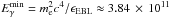 eV ~ Eb2 was introduced, meaning the minimum energy of a primary γ-ray that undergoes effective absorption on EBL photons. The corresponding energy of electrons of the produced pair are
  . Secondary γ-rays produced by electrons with energy
  typically have energy
  (Blumenthal & Gould 1970). Putting together the expressions for EX,
  , and ,
  .
.
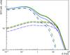 |
Fig. 7 Observable SED for various Ep0 (solid curves): black curve – Ep0 = 10 EeV, red – 30 EeV, green – 50 EeV, blue – 100 EeV. SEDs decomposed on the contributions from the primary cascade particles produced at z< 0.06 (dashed curves) and at z> 0.06 (dot-dashed curves) are also shown. |
We denoted the number of cascade electrons that have energy Ee during the whole time of cascade development as qe(Ee). We took into account that the number of electrons in each cascade generation, Ne ≈ 2Nγ, and the energy of these electrons, ≈ Eγ/ 2, has nearly the same distribution as the energy of the γ-rays of the same generation. Therefore, qe(Ee) ∝ 1 /Ee for the  energy range (as qe·Ee ∝ the primary energy E0). Most electrons are produced above , therefore in the low-energy range
  qe(Ee) ≈ const. Finally, the spectrum of cascade photons may be found from the following equation: dnγ(Eγ) = qe(Ee)dEe/Eγ. Again using the expression for secondary γ-ray energy
  , for (corresponding to Eγ<EX) we obtain for the shape of the observable spectrum
  , which is similar to
  . Similarly, for
  the shape of the observable spectrum is
  . Numerical simulations performed in Berezinsky & Kalashev (2016) indicate
  in the same energy region. The simplified analytic model considered above assumes that all primary γ-rays with energy
  are completely absorbed and, consequently, the spectrum has an abrupt cutoff at this energy. By detailed numerical calculations presented here we reproduce the more realistic shape of the high-energy cutoff, both for primary γ-rays and primary protons.
Figure 7 shows observable SEDs for different values of Ep0. For Ep0 = 10, 30, 50 EeV the shape of the spectra are nearly identical, whereas for the case of Ep0 = 100 EeV the spectrum is somewhat steeper due to a pile-up of the w(z) dependence near the source of primary protons. Indeed, in the latter case more energy is injected near the source, thus more electromagnetic cascades start to develop at comparatively high distance from the observer, thus leading to lower intensity at high values of the observable energy.
Different components of the observable SEDs are also shown in Fig. 7: the one formed by γ-rays and electrons that were produced by primary protons at z< 0.06, and the other contribution for z> 0.06. The first component dominates at E> 5 TeV and has almost the same shape of the spectrum for all Ep0 considered. This effect may be qualitatively understood as follows. The spectrum of the first component is defined by an equation similar to Eq. (7), but with limits of integration on the redshift equal to 0 and 0.06. Primary protons with energy >50 EeV quickly lose energy to pion production (see Berezinsky et al. 2006) until they reach the energy range where pair-production losses dominate. Therefore, Kem(z) ~ 1 at z<0.06 even for Ep0 = 100 EeV (Fig. 5). The w(z) dependence is also similar for all considered Ep0 at z< 0.06 (Fig. 4). Again, this is due to the fact that for Ep0> 50 EeV protons quickly lose energy so that their energy at z< 0.06 is similar irrespective of the Ep0 value. Thus, the shape of the observable SEDs at E> 20 TeV, where the first component is strongly dominant, is almost the same. In the 200 GeV−10 TeV energy region and when Ep0 = 100 EeV, the first component has lower relative normalization with respect to the second component, once again due to the fact that in this case a larger fraction of primary energy is lost at z> 0.06 than for Ep0< 50 EeV. The second component for Ep0 = 100 EeV is also somewhat steeper for Ep0 = 100 EeV due to the same effect. Therefore, the overall observable SED in the 200 GeV−10 TeV energy region is steeper for Ep0 = 100 EeV than for the other considered values of Ep0. The difference in the slope between the observable SEDs in this energy range may be estimated as follows. The total normalization of the second component is 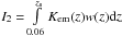 , and of the first component is
 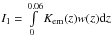 . Knz = CnzI1/I2 is the ratio of these quantities for which the normalization factor Cnz is chosen so that Knz = 1 at Ep0 = 30 EeV. Direct numerical calculation yields the values Knz = 0.91 at Ep0 = 10 EeV, Knz = 1 at Ep0 = 30 EeV, Knz = 1.01 at Ep0 = 50 EeV, and Knz = 0.63 at Ep0 = 100 EeV. These values translate to the difference in the power-law slope δγ = 0.07−0.09 between the case of Ep0 = 100 EeV and other cases.
2.2.2. Observable γ-ray spectra in the full hybrid approach
To obtain the observable spectrum without the assumption of cascade universality, we calculated an array of cascade spectra from primary γ-rays and electrons of energies 10 TeV–100 EeV. From 10 TeV to 10 EeV the power-law slope indices of the primary spectra of these cascades (dN/ dE0) were set to γ0 = 1, and from 10 EeV to 100 EeV – to γ0 = 2. As in the universal spectrum approach, we propagated primary protons, but now, instead of the universal spectrum, we utilized our new database of cascade spectra. We calculated a vast two-dimensional array of secondary particle spectra for the case of the pair production process, as described above, and for the photopion process for γ, e+, νe, νμ, . In both cases we calculated these spectra for the case of one hundred and one logarithmically spaced values of Ep from 1 EeV to 100 EeV, and for thirty linearly spaced values of z from 0 to 0.30. These arrays were used to calculate the observable γ-ray spectrum, that is:
where (dN/ dE)e−c(Es,E,z) and (dN/ dE)γ−c(Es,E,z) are, as before, the spectra of cascades, but now the shape of these spectra may depend not only on z, but also on the primary energy Es and the type of the primary particle. In these equations (dN/ dEs)e−p(Es,z) and (dN/ dEs)γ−p(Es,z) are the spectra of secondary electrons and γ-rays, respectively, that were produced by primary protons.
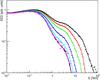 |
Fig. 8 The comparison between observable SEDs obtained in the full hybrid approach (circles) and the universal hybrid method approach (solid curves) for different values of the zc parameter: black – zc = 0, red – zc = 0.02, green – zc = 0.05, blue – zc = 0.10, cyan – zc = 0.15, magenta – zc = 0.18. Primary proton energy Ep0 = 30 EeV. The universal spectrum for the case of primary γ-rays with energy 1 PeV is shown for comparison (dashed black line). Relative normalization of all spectra is done at E = 10 GeV. |
The results of our calculations of observable SEDs are presented in Figs. 8−11. The comparison graph of spectra calculated with two different approaches for the case of Ep0 = 30 EeV (Fig. 8) shows very good agreement. We also considered the possibility of a highly-structured extragalactic magnetic field, such as a galaxy cluster, that is situated at some redshift zc between the source and the observer. We assume that the magnetic field strength in this cluster is sufficiently high such that the proton beam traversing the cluster is practically dissolved. Several cases of observable spectra for different zc are also shown in Fig. 8. In all these cases the agreement of results obtained with two different approaches is good. Finally, Fig. 8 shows that in the case when zc ≈ zs, the observable spectrum is very similar to a universal cascade spectrum from primary γ-rays. The same SEDs, but without relative normalization, are shown in Fig. 9.
Observations of extreme TeV blazars used in this paper.
The same results as in Fig. 8, but for Ep0 = 100 EeV, are shown in Fig. 10. For zc ≤ 0.05 the agreement between the results obtained with our two methods is very good, whereas for zc ≥ 0.10 the SEDs resulting from the universal hybrid approach are steeper at comparatively high values of observable energy, E> 500 GeV. This property of observable SEDs is possibly due to a hardening of the electromagnetic cascade spectra shape for the case of high primary energy, Eγ0 ≥ 1 EeV, see Fig. A.3. This hardening is the result of the “extreme high-energy cascade regime” that is realized when Eγ0ϵ ≫ mec2, where ϵ is the energy of EBL/CMB photon, and me is the mass of electron. In this regime, for the case of the pair production process one electron of every produced pair gets almost all of the energy of the primary photon and the secondary photon in the IC process likewise gets almost all of the energy of the primary electron (for comparatively recent discussions see Khangulyan et al. 2008; Aharonian et al. 2012). As a result, the electromagnetic cascade develops much more slowly than in the universal regime.
We note, however, that the ELMAG code accounts neither for a possible impact of the so-called universal radio background (URB) upon the cascade development (Protheroe & Biermann 1996; Settimo & De Domenico 2015), nor for the higher-order quantum electrodynamics (QED) processes such as double pair production (e.g. Brown et al. 1973; Demidov & Kalashev 2009) or “triplet production” (Mastichiadis et al., 1994). The results presented in Settimo & De Domenico (2015; Fig. 2, bottom) show that the mean free path for the IC process is likely to be affected by these effects even for the primary electron energy of 10 EeV, thus making the “extreme high-energy cascade regime” less pronounced. In what follows we mainly use results obtained in the universal cascade regime. Finally, the same SEDs as in Fig. 10, but without relative normalization, are shown in Fig. 11.
3. The sample of blazar spectra
In this study we focus on a subsample of AGN, the so-called extreme TeV blazars (Bonnoli et al. 2015). Blazars are defined as a class of AGN that have peculiar multi-wavelength properties from radio to γ-ray bands of the spectrum. From the point of view of a γ-ray astronomer, a blazar may be defined simply as an AGN that is a bright source of γ-ray emission. Extreme TeV blazars are believed to have particularly high peak-energy in their SED, meaning Epeak> 1 TeV (Bonnoli et al. 2015).
During the last decade, these sources have become very important for the studies of γγ absorption on EBL (Aharonian et al. 2006). Indeed, these sources allow us to study this effect for the highest values of τγγ available now. Additionally, they may have a very hard primary spectrum of γ-rays, thus making the contribution of the cascade component significant even in the VHE energy range.
The sample of observations of extreme TeV blazars used in this paper is presented in Table 1. It contains nine independent observations of six sources, performed with imaging Cherenkov telescopes HEGRA, CAT, Whipple, H.E.S.S., and VERITAS. For the whole history of observations of these sources in the VHE energy region up to 1 Jan. 2016 (Wakely & Horan 2016), five out of six of them display a very slow, if any, variability, with characteristic periods of months or even years. The only exception is 1ES 1812+304; for this source a rapid flare with a full width at half maximum of about two to three days was observed in 2008 by the VERITAS telescope 2010.
4. Fitting the spectra of extreme TeV blazars
In this section we compare the predictions of different models with observations. Before we proceed to present the fits for various sources, we wish to make some remarks. The collaborations operating the Cherenkov telescopes usually reconstruct the spectrum of primary γ-rays, not just the histogram of measured energy values. Therefore, while presenting our results, we will not perform any convolution of model spectra with instrumental energy resolution templates. Of course, the procedure of the primary spectrum deconvolution always results in some additional systematic uncertainty of the reconstructed spectrum. However, these systematic uncertainties are usually subdominant in Table 1, especially in the optically-thick region, to which we pay most attention in this work.
Another remark concerns the selection of the EBL model for the case of absorption-only fits. Meyer et al. (2012) calculate the significance Za of the VHE anomaly for different EBL models (Franceschini et al. 2008, hereafter F08; Kneiske & Dole 2010, already denoted as KD10), and Dominguez et al. (2011, D11) and find that Za may depend non-trivially on the total normalization of the EBL intensity in a certain wavelength band. The lowest Za is obtained for the case of the F08 model. Therefore, in what follows we present absorption-only fits using the F08 model. For comparison, we also include the fits for the G12 model and the model directly derived from the ELMAG code (see next subsection for more details).
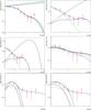 |
Fig. 12 Model fits for the case of 1ES 0347-121. Red circles denote measurements, bars – their uncertainties; long-dashed lines – primary γ-ray spectra. Top-left – absorption-only model: black – G12 EBL model, green – F08, blue – KD10 model as implemented in ELMAG; solid lines – observable spectra. Top-right – electromagnetic cascade model: blue solid line denotes observable spectrum, black – absorbed component, green – cascade component. Middle-left: the same as for top-right, but showing the high-energy cutoff of the primary spectrum. Middle-right – basic hadronic model: black solid line denotes zc = 0, magenta – zc = 0.02, green – zc = 0.05, blue – zc = 0.10; short-dashed line – power-law spectrum of primary protons with zc = 0. Bottom-left – modified hadronic model, the same meaning of colours as in the middle-left panel. Bottom-right – another fit for the case of modified hadronic model. |
4.1. The case of 1ES 0347-121
We start our discussion with the case of blazar 1ES 0347-121 and the absorption-only model. The redshift of this source, z = 0.188, is very near to 0.186, for which all calculations presented in Sect. 2 are applicable. The shape of the primary spectrum was chosen as: 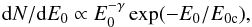 (11)where E0c is the cutoff energy. For this model we neglected adiabatic losses, because they do not change the shape of the spectrum.
The ROOT analysis framework with the integrated minimization system MINUIT (James & Roos 1975), specifically the gradient optimization routine MIGRAD, was used to obtain this fit. During the optimization procedure, every experimental bin was divided into twenty small parts and the flux extinction factor that is proportional to exp(−τ) was calculated for each of these sub-bins to ensure realistic implementation of the γ-ray absorption process. After that, a histogram of the model SED was evaluated, and a χ2 minimization was performed with the MIGRAD routine. The output of the routine includes the optimized values of the primary spectrum parameters.
The result of fitting the absorption-only model is shown in Fig. 12, top-left panel. We note that this and the following spectra are presented in the form of histograms with dense energy-sampling using narrow model bins, instead of the somewhat sparse experimental histograms that were in fact computed during the optimization procedure. Together with fits for the case of the G12 and F08 EBL models, we present a similar result for the case of the EBL model as implemented in ELMAG. To do this, we evaluated optical depth vs. energy for this model as: 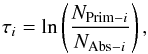 (12)where i is the number of bin in the energy histogram; NPrim is the histogram of primary photons, but redshifted to account for adiabatic losses; and NAbs is the histogram of detected photons, that were not absorbed, meaning that i corresponds to a certain narrow interval of observable energies for both histograms. Appendix C demonstrates that for the case of the KD10 model the ELMAG code slightly, about 10−20%, overestimates τ in the 1−10 TeV energy range. However, because the actual EBL level is still uncertain, this EBL model that differs from the original KD10 model is still perfectly acceptable for our study.
Top-right panel of Fig. 12 presents a fit in the framework of the electromagnetic cascade model of Dzhatdoev (2015a,b). To obtain this fit, we generated a large array of cascades from primary γ-rays, using the ELMAG code with the power-law spectrum d and primary energies from 100 GeV to 100 TeV. Observable spectra for any other primary spectrum of γ-rays dNprim/ dE0 may be calculated using a re-weighting procedure with a weight defined as:
  (13)To test this spectrum synthesis procedure we present a comparison graph (see Appendix D, Fig. D.1) that compares spectra calculated by Vovk et al. (2012) using the F08 EBL model and our results obtained with the primary spectrum parameters from Vovk et al. (2012). Notwithstanding slightly different EBL models, the agreement between the total observable model spectra is very good.
As for the case of the absorption-only model, we generated histograms of observable spectra for a set of parameters, γ,Ec, and performed optimization over these parameters. This time we evaluated χ2 on a grid of 10 × 10 cells with exhaustive calculation. The values of γ,Ec that ensure the minimal value of χ2 on this grid were found, and the optimization run was repeated on a similar grid, but with a smaller step (δγ,δEc). This procedure was repeated several times until δγ< 10-2 and δEc< 0.1 TeV. The step-decreasing factor was set to three. We put considerable effort into ensuring that the global minimum of χ2 was captured by our optimization method.
The best-fit spectrum consists of two distinct components, namely the primary, absorbed, component that dominates at high energy, and the cascade component that has a somewhat steep spectrum and contributes mainly in the low-energy region of the total spectrum. These two components, when put together, produce an ankle-like spectral feature at an energy of around 1 TeV. The same fit, but with different energy and intensity scale, is shown in Fig. 12, middle-left panel. It is clearly seen that the cutoff in the primary spectrum is situated well below 100 TeV.
Figure 12, lower-left panel, was calculated for the case of the “basic hadronic cascade model” of Essey et al. (2010b), in which all observable γ-rays are of secondary nature, meaning that they were produced by protons on the way from the source to the observer. Apart from the option without any considerable EGMF on the line-of-sight, we also included several options with a possible magnetic field structure at zc, as was described in Sect. 2.2.2.
These sorts of results shown in the present section were obtained in the weak universality approximation with Ep0 = 30 EeV. The case of the power-law spectrum of primary protons from 1 EeV to 100 EeV with  is also included in this figure.
The case of the “modified hadronic cascade model” (Essey & Kusenko 2014) that includes both primary and secondary components is shown in two lower panels of Fig. 12. Optimization was performed on four parameters: the normalization factors of the primary γ-ray and cascade components, and the parameters of the shape of the primary component (γ,Ec) (see Eq. (11)).
An exhaustive search is extremely time-consuming on this kind of a four-dimensional grid. Therefore, we have developed a code in the ROOT framework using the Minuit package to perform gradient optimization. The formal best fit obtained with this procedure is presented in Fig. 12, bottom-left. For the case of the primary γ-ray component we neglected weak cascade emission produced by this component. In this case the spectrum of the primary component appears to be very narrow, with sharp lower- and higher-energy cutoffs. In Fig. 12, bottom-right, we show, however, that even in the case of a more realistic primary component a good fit to the observed SED is obtainable.
We now introduce a quantity called the modification factor (following Berezinsky et al. 2006), also known as the flux boost factor (Sanchez-Conde et al. 2009), which is defined as the ratio between the spectra in the electromagnetic cascade model (ECM) and the spectra in the absorption-only model (AOM):  (14)The graph of KB(E) for blazar 1ES 0347-121 and the KD10 EBL model, as implemented in the ELMAG code, is shown in Fig. 13. For calculations of the boost factor, (dN/ dE)ECM and (dN/ dE)AOM were interpolated to 1000 bins. KB(E) is clearly greater than unity for E> 2 TeV; the ratio of the maximal to the minimal values of KB(E) is about 3.5. Therefore, the electromagnetic cascade model predicts that the intensity in the optically-thick region may significantly exceed the value deduced from the fitting of the optically-thin part of experimental SED in the framework of the absorption-only model. Indeed, the cascade component, dominating at low energies, ensures good quality of fit at these energies, notwithstanding a very hard primary spectrum. In effect, the cascade component conceals, or “masks”, the primary component in the optically-thin energy region, hence the name of the present paper. On the other hand, at high energies where τ> 2, a very hard primary spectrum provides enough photons to explain observations even after extinction caused by the EBL.
4.2. The case of 1ES 0229+200
Blazar 1ES 0229+200 is a frequent source in many discussions of extragalactic γ-ray propagation due to its hard spectrum, slow variability, and comparatively high total flux. The fits for the case of the absorption-only model, which are similar in every respect to those presented in Fig. 12 for 1ES 0347-121, are shown in top-left panel of Fig. 14.
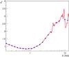 |
Fig. 13 Flux boost factor KB(E) for 1ES 0347-121 (red curve). Blue circles – KB(E) averaged over energy intervals to suppress statistical fluctuations. |
For this source we also present two fits for a model that includes the γ → ALP oscillation process (top-right panel of Fig. 14), but without account of any secondary, cascade, emission. As was discussed in the introduction (Sect. 1), extra photons with respect to the case of the absorption-only model in the optically-thick region of the spectrum may be ascribed to this process. To evaluate the effect of γ-ALP mixing in the spectrum of 1ES 0229+200, we used the results of Sanchez-Conde et al. (2009) that were calculated for a similar z = 0.116. Sanchez-Conde et al. (2009) presented graphs for the boost factor (Fig. 7 of their work) for the case of the Primack et al. (2005) EBL model, as well as for the Kneiske et al. (2004) EBL model. In the former case, the values of KBoost in the optically-thick region are typically smaller than in the latter case. These two cases, weak and strong flux enhancement, respectively, serve to qualitatively demonstrate more or less strong γ-ALP mixing effects. However, in Fig. 12 we actually use the fixed EBL model G12.
More detailed study of γ-ALP mixing is underway and will be reported elsewhere. Given huge uncertainties of EGMF strength and a vast range for the γ-ALP mixing parameter values, we find it appropriate to use these estimates, even though they were derived for the case of a slightly different redshift and different EBL models.
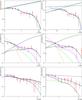 |
Fig. 14 Model fits for the case of 1ES 0229+200. Top-left – absorption-only model, all notions are the same as in Fig. 11, top-left. Top-right – comparison of the absorption-only and γ-ALP mixing models: black line denotes absorption-only model, green – weak γ-ALP flux enhancement, blue – strong γ-ALP flux enhancement. Middle panels – electromagnetic cascade model for the case of the VERITAS (left) and H.E.S.S. (right, red triangles) observations together with cascade spectra for monoenergetic primary γ-ray injection (short-dashed lines): red – Eγ0 = 10 TeV, blue – Eγ0 = 100 TeV, magenta – Eγ0 = 1 PeV. Bottom-left – basic hadronic cascade model (zc are the same as in Fig. 12 middle-right); bottom-right – modified CR beam model. |
It is interesting that the case of weak mixing is practically indistinguishable from the absorption-only model fit. The primary spectrum in the case of the exotic model is indeed less hard than without it, but that does not induce any significant observable effect in the 300 GeV−10 TeV energy range. Moreover, the difference between the spectra in these two cases is clearly insufficient to choose between the models on purely astrophysical grounds. On the other hand, in the low-energy range, together with a spectral irregularity at E = 20−30 GeV that was qualitatively discussed in introduction, another feature is present, namely the spectral slope for the case of exotic model is steeper than the one for the absorption-only fit, reflecting the shape of the primary spectrum. Therefore, it appears that for the case of weak mixing the observable spectrum is the same or even steeper at all energies from the above-mentioned irregularity up to 10 TeV, and never harder. To our knowledge, this highly unexpected result was never reported before.
For the case of strong mixing the situation is different. The intensity of the observable model spectrum at E> 3 TeV is greater than the ones calculated for the case of the absorption-only model and the case of weak mixing, although all other features of the spectrum are qualitatively similar. However, according to Ajello et al. (2016), this strong mixing regime was strongly constrained considering the non-detection of the low-energy spectral irregularity, as was discussed in the introduction. The fits for the case of the electromagnetic cascade model are presented in the middle panels of Fig. 12 for the case of VERITAS (left) and H.E.S.S. (right) observations. In both cases the ankle feature, which is formed by the intersection of the primary, absorbed, and secondary, cascade components, is clearly seen. The position of the ankle is similar for both cases, again indicating that this feature, however faint, is not just a statistical fluctuation. For comparison, cascade spectra for the case of monoenergetic primary injection with various energies are also shown. Finally, the low panels of Fig. 14 were computed for the case of the basic (left) and modified (right) hadronic cascade models. Both VERITAS and H.E.S.S. data are presented in the picture, with normalization to the H.E.S.S. data. The fits of low panels of Fig. 14 were obtained using exactly the same procedure as those presented in Fig. 12, middle-right and bottom-left. In Appendix D, Fig. D.2 we present a comparison graph of spectra calculated for the basic hadronic model by Essey et al. (2011) and Murase et al. (2012), and by us for the case of zs = 0.14.
For 1ES 0229+200 we also present several fits for the case of a simple model of structured EGMF. Namely, following Furniss et al. (2015), we use the voidiness parameter VLoS, which is defined as the ratio of the comoving line-of-sight distance covered by underdense regions of space (voids) to the total line-of-sight distance from the source to the observer. In fact, a spatial region that is comparatively close to the source (typically 10−100 Mpc from the source) is the most important for cascade development, because it contains most of the cascade electrons. EGMF strength in voids may be sufficiently low to allow cascade electrons to radiate secondary photons before the electrons are strongly deflected from the line-of-sight. On the contrary, denser regions of space, as compared to voids, typically contain comparatively strong magnetic fields B ~ 10-6−10-11 G. Cascade electrons produced in these regions are strongly deflected and delayed, and secondary photons do not contribute to the observable spectrum. In effect, to account for possible structures within a strong magnetic field, we multiply the cascade component by the suppression factor 0 <KV< 1.
Several fits to the spectrum of 1ES 0229+200 for different values of KV, from 0.2 to 1.0, are presented in Fig. 15. The corresponding graphs of boost factor for these fits are shown in Fig. 16. This figure demonstrates that the ankle signature in the total model spectrum does not disappear for KV< 1, but, on the contrary, only gets more prominent as KV falls in the range of the considered KV values.
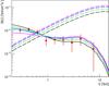 |
Fig. 15 Fits to the spectrum of 1ES 0229+200 for the electromagnetic cascade model and different values of KV. Dashed lines denote a primary spectrum near the source, solid lines – total model spectra; black – KV= 1, green – 0.6, blue – 0.4, cyan – 0.3, magenta – 0.2. |
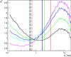 |
Fig. 16 Boost factor KB vs. energy for the fits presented in Fig. 13. Solid lines denote KB(E) for different values of KV: black – KV = 1, green – 0.6, blue – 0.4, cyan – 0.3, magenta – 0.2. Dashed vertical lines denote the energy corresponding to τ = 1: black for the G12 EBL model, red – KD10, green – F08, blue – KD10 as implemented in the ELMAG code. Solid vertical lines denote the energy corresponding to τ = 2 (the same meaning of colours as for dashed vertical lines). |
4.3. The case of 1ES 1101-232, 1ES 1812+304, 1ES 0414+009, and H 1426+428
1ES 1101-232 was observed by the H.E.S.S. Collaboration in 2004−2005, and the result of spectral measurements was published in Aharonian et al. (2006). One year later, a reanalysis of these observations was performed, and the new result on the spectrum was presented in Aharonian et al. (2007b).
In our work we mainly use the latter results, but we also present a fit for the case of the electromagnetic cascade model for the former analysis. Figure 17, top-left panel, contains a fit to the SED of 1ES 1101-232 in the absorption-only model. The top-right and middle-left panels of Fig. 17 contain the fits for the case of the electromagnetic cascade model for reanalysis and 2006 analysis, respectively.
A basic hadronic model fit is presented in Fig. 17, middle-right panel. The formal best fit for the case of the modified hadronic model is shown in Fig. 17, bottom-left. As for the case of 1ES 0347-121, the primary component in this figure is very narrow. Therefore we also present another, more physically plausible fit for the same model in bottom-right panel of Fig. 17.
Similar fits for 1ES 1812+304 and 1ES 0414+009 are shown in Fig. 18. The spectrum of 1ES 1812+304 is not far from the case of the universal spectrum of γ-rays. In the framework of the basic hadronic model this corresponds to the case of zc, which is only slightly less than z of the source.
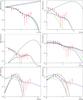 |
Fig. 17 Model fits for the case of 1ES 1101-232. Top – the absorption-only model (left) and the electromagnetic cascade model for the case of 2007 reanalysis (right); all notions are as in corresponding panels of Fig. 10. Middle-left – electromagnetic cascade model for the case of 2006 analysis. Middle-right – basic hadronic cascade model in which zc are the same as in Fig. 10 middle-right. Bottom-left and bottom-right – modifed hadronic model (details in the text). |
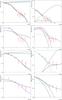 |
Fig. 18 Model fits for the case of 1ES 1218+304 (first row, left – absorption-only model; first row, right – electromagnetic cascade model; second row, left – basic hadronic model (black curve – zc = 0, blue curve – zc = 0.15); second row, right – modified hadronic model) and 1ES 0414+009 (third row, left – absorption-only model; third row, right – electromagnetic cascade model; bottom-left – basic hadronic model (black curve – zc = 0, blue curve – zc = 0.25); bottom-right – modified hadronic model). |
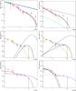 |
Fig. 19 Model fits for the case of H 1426+428. Top-left – absorption-only model, top-right – electromagnetic cascade model (formal best fit). Middle panels – two fits for the electromagnetic cascade model with large contribution of cascade component at low energy. Bottom-left – basic hadronic model (black curve denotes zc = 0, blue curve – zc = 0.1), bottom-right – modified hadronic model. |
Finally, fits for the source H 1426+428 are shown in Fig. 19. For this object, the formal best fit for the electromagnetic cascade model is practically coincident with the case of the absorption-only model. The contribution of the cascade component to the total flux in this case is vastly subdominant, only a few percent. In this respect, it is interesting that Furniss et al. (2015) estimated VLOS ~ 0 for this source, meaning that there is little room on the line of sight where an electromagnetic cascade could develop. Nevertheless, we also present two fits for the case of a dominant cascade contribution at low energy (E< 1 TeV), for completeness. The fits for the case of basic and modified hadronic model are presented as well.
5. Constraints on hadronic cascade models
As we have seen in the previous section, both electromagnetic and hadronic cascade models provide reasonable fits to the observed shape of the spectra of the extreme TeV blazars considered in this paper. Some additional information is required to favour one model over another. One of the criteria upon which this could be done is the plausibility of the source emission model in the context of the total normalization of a certain emission component. Tavecchio (2014) developed this kind of a model, hereafter the T14 model, specifically for the hadronic cascade scenario. In what follows we use the parameters of blazar emission presented in Tavecchio (2014, Table 2).
In fact, the central emitting object of a blazar is circumvented by magnetic fields of an appreciable strength and spatial scale. In what follows we assume the model of the galaxy cluster turbulent magnetic field of Meyer et al. (2013), Eqs. (14), (15) with parameters rcore = 200 kpc, β = 2/3, η = 1/2, coherence scale 10 kpc (the spatial dimensions of all magnetic field domains are equal), and variable parameter  (hereafter denoted simply as B0).
These magnetic fields modify the angular pattern of the proton beam, thus effectively dimming the observable emission. The initial angular pattern of the hadronic beam was set to be the same as the angular pattern of the leptonic component. The T14 model provided the following constraint to the total power of proton emission: it cannot be greater than the total “magnetic luminosity” PB. Indeed, in the context of the T14 model, protons during the acceleration are confined to the region of the magnetic field. Therefore the energy density of these protons can not be higher than the energy density of the magnetic field, otherwise they escape from the region, thus terminating the acceleration process. The T14 model introduced a parameter of the maximal proton acceleration energy, Emax. We assume the accelerated proton spectrum shape dNp/ dE ∝ E− γpexp(−Ep/Emax).
It is convenient for us to count the total power of accelerated protons Lp with respect to the power-law spectrum, introducing an additional factor 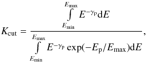 (15)so that Lp<KcutPB. In what follows we introduce additional modification factors of the proton intensity with respect to the power-law spectrum of protons dNp/ dE ∝ E− γp. We set Emin = 1 EeV and Emax = 100 EeV.
We estimate the flux modification factor KM as: 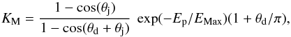 (16)where θj = 1/Γ, Γ is the bulk Lorentz factor of the blazar jet. The deflection angle of protons in the cluster magnetic field is estimated as:
  (17)where N = 200 is the number of magnetic field domains and θi are partial deflections of proton in these domains:
 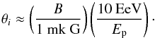 (18)This approximation works reasonably well in the small deflection angle limit, θd ≪ 1 rad. As we will see, the small deflection angle assumption is also well justified.
The interpretation of Eq. (16) is as follows: the jet angular pattern is broadened by the deflection of protons in the cluster magnetic field; high energy protons at Ep>Emax effectively leave the region of acceleration and only a small number of particles are accelerated far above Emax; and the factor (1 + θd/π) roughly accounts for the effect of the visibility of the second jet, the counter-jet, when the deflection angle is large. The modification factor for the case of several values of the B0 parameter is shown in Fig. 20.
After that, we calculated the spectrum of observable γ-rays for different model parameters. We assume that all energy of the secondary electrons and photons was converted to the energy of cascade γ-rays. Because we are interested only in setting an upper limit to the intensity of the observable γ-rays produced by protons on the way from the source to the observer, this assumption is justified.
In this section we consider the intermediate hadronic cascade model with different values of the zc parameter. We performed absolute normalization of the spectrum using the T14 model. We considered the source 1ES 0229+200 and two options for model parameters presented in T14, the one corresponding to Γ = 10 and the one corresponding to Γ = 30. The object 1ES 0229+200 is an archetypal extreme TeV blazar that was considered in Essey & Kusenko (2010b) as a very good candidate for the basic hadronic model. Figure 21 presents normalized observable γ-ray spectra for zc = 0 and the same values of the B0 parameter as in Fig. 20.
Finally, we performed an exhaustive scan over a wide range of parameters, including zc and B0, on a 200 × 200 grid for two options of the source emission models presented in T14, labelled by the values of Γ = 10 and Γ = 30. Using a simple χ2 goodness-of-fit statistical test, for every version of the observable spectrum we calculated a p-value according to the prescriptions of Beringer et al. (2012). After that, these p-values were converted to Z-values (i.e. statistical significance) according to the prescriptions of Beringer et al. (2012). Figure 22 shows Z-values in colour. It was drawn for the case of Γ = 10, and Fig. 23 was drawn for the case of Γ = 30. All values of Z> 10σ were set to 10σ. The lower-left parts of Figs. 22, 23 correspond to the case when the intensity of the observable γ-rays is much greater than the one required by observations. Other parts of these graphs denote the range of acceptable models. Finally, the upper-right parts of these graphs display the regions of parameters where the corresponding model is excluded. It is remarkable that all considered configurations with B0 above 100 nG are excluded with significance Z> 7σ.
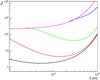 |
Fig. 20 Modification factor KM for different values of B0. Black curve denotes B0 = 1 nG, red curve – 10 nG, green – 100 nG, blue – 1 mkG, magenta – 10 mkG. |
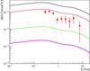 |
Fig. 21 Model spectrum for different values of B0. Colours denote the same values of B0 as in Fig. 20. |
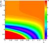 |
Fig. 22 Significance (Z-value) of the intermediate hadronic model exclusion for Γ = 10 and blazar emission parameters from T14. |
During this calculation it should be remembered that we neglected the losses of protons on the EBL from the source to the observer. However, there are two main factors that strongly outweigh this one, namely: 1) the injection of protons in the context of the T14 model is done at an energy Ep−inj much lower than 1 EeV. Therefore, for the case of Ep−inj= 10 GeV and γp = 2, the total energy of accelerated protons is five times greater than the energy of ultrahigh energy (UHE) protons and thus the modification factor in this case decreases by the factor of five; and 2) synchrotron and curvature-radiation losses of primary UHE protons will futher diminish their total energy. The second factor is particularly strongly constraining for the case of the Blandford-Znajek emission mechanism (Blandford-Znajek 1977) due to strong magnetic fields in the acceleration region, see Neronov et al. (2009) and Neronov & Ptitsyna (2016).
6. Summary and conclusions
In this work we reviewed the main possibilities of how cascades from primary γ-rays or protons may influence the data interpretation when testing extragalactic γ-ray propagation models, mainly dealing with the source redshift range 0.1–0.3. We reviewed the main regimes of electromagnetic cascade development: 1) one-generation regime, which holds when Eγ0< 10 TeV; 2) the universal regime, which is satisfied when Eγ0> 100 TeV; and 3) a possibility of the extreme energy cascade regime at Eγ0> 1 EeV.
We developed a fast, simple and suffuciently precise hybrid code that allows us to calculate the observable spectrum of γ-rays for the case of primary protons. We performed calculations of observable spectra for this case and investigated several versions of the hadronic cascade model: the basic model, in which all γ-rays are generated by primary protons; the intermediate model, which is the same but the proton beam is dissolved at some zc, such that the basic model is the sub-set of intermediate models with zc = 0; and the modified model that includes the primary component. We discuss the signatures of the spectrum for the basic hadronic model for zs = 0.186. The signatures at a comparatively low observable energy are almost the same as the ones for the case of a purely electromagnetic cascade, that is, the E-1.60dN/ dE spectrum below ~ 200 MeV and E-1.85 spectrum from ~ 200 MeV to ~ 200 GeV. However, at higher energy (E> 200 GeV) the spectrum in the hadronic model is much harder than the universal spectrum for the case of a pure electromagnetic cascade.
We also compare two hybrid calculations of observable spectra for different values of zc from 0 up to nearly zs. The results of these calculations with two different methods are in very good agreement for the case of the proton primary energy Ep0 ≤ 30 EeV, meaning when the pair-production losses are dominant. For the case of Ep0 = 100 EeV, the agreement between the two methods is also good for the basic hadronic model and the intermediate hadronic model with comparatively low zc<zs/ 2, but not so good if zc ≥ zs/ 2. The reason for this disagreement may be connected to the possibility of the extreme energy cascade regime. New calculations and measurements of the universal radio background are necessary to decide which spectrum is more realistic. Although we confirm the claim that the shape of the observable spectrum in the basic hadronic model depends only slightly on the primary proton energy, we find that in the context of the intermediate hadronic model the shape of the spectrum strongly depends on the zc parameter in the high energy region.
We performed a series of fits to the spectra of extreme TeV blazars with various extragalactic γ-ray propagation models, namely: the absorption-only model, the electromagnetic cascade model, the basic hadronic model, the intermediate hadronic model, and the modified hadronic model. Most of the fits presented in this paper are formal best fits. We find that, as a rule, both the electromagnetic cascade model and the hadronic cascade model are able to provide a reasonable fit to the observed spectral shape.
For the case of blazar 1ES 0347-121 and the electromagnetic cascade model, we performed the calculation of modification factor KB with respect to the absorption-only model. We find that KB> 1 in the energy region of 1−10 TeV. Therefore, the version of the electromagnetic cascade model that was considered in this work for this source predicts that it is possible that the observable intensity is higher than in the absorption-only model for the same level of EBL without any new physics. For the case of the source 1ES 0229+200 we also performed a fit in the framework of an exotic model with γ → ALP oscillations, and a calculation of the modification factor KB vs. voidiness KV dependence in the framework of the electromagnetic cascade model. We find that when KV is lower than one the value of KB does not fall at high energies, but, on the contrary, even grows in the energy range of 1−15 TeV, thus making the effects induced by electromagnetic cascades even more pronounced.
Finally, using the fact that many blazars are situated in galaxy groups or clusters with comparatively strong magnetic fields (Muriel 2016; Oikonomou et al. 2014), we performed the testing of the emission model of Tavecchio (2014). We find that for B0> 100 nG this emission model is excluded with significance Z> 7σ. Our results show that the hadronic cascade model experiences significant difficulties. This conclusion is in line with results obtained by Razzaque et al. (2012). Further testing of the hadronic and electromagnetic cascade models may be performed on an event-by-event level with advanced analysis tools such as GammaLib and ctools package (Knoedlseder et al. 2016). This sort of work is underway in our group.
We conclude that cascades from primary γ-rays or nuclei may induce an appreciable background for astrophysical searches for γ−ALP oscillation that needs to be taken into account. The electromagnetic and hadronic cascade models deserve further study, also in the context of searches for other exotic phenomena, such as Lorentz invariance violation (Tavecchio & Bonnoli 2016). The knowledge of EGMF would provide a significant insight into the intergalactic cascade phenomena in the Universe. Further measurements with the CTA array of Cherenkov telescopes (Acharya et al. 2013) will likely clarify these issues. Together with the existing instruments Fermi LAT (Atwood et al. 2009) and AGILE (Rappoldi et al. 2016), future experiments that have either high sensitivity or good angular resolution, such as GAMMA-400 (Galper et al. 2013) or the novel balloon-borne emulsion γ-ray telescope GRAINE (Takahashi et al. 2015), may also prove to be helpful in this task.
Acknowledgments
This work was supported by RFBR, Grant 16-32-00823. The authors are grateful to Dr. V. V. Kalegaev for permission to use the SINP MSU space monitoring data center computer cluster and to V. O. Barinova, M. D. Nguen, D. A. Parunakyan for technical support.
References
- Abdo, A. A., Ackermann, M., Ajello, M., et al. (Fermi-LAT Collaboration) 2011, ApJ, 727, 129 [NASA ADS] [CrossRef] [Google Scholar]
- Abramowski, A., Acero, F., Aharonian, F., et al. (H.E.S.S. Collaboration) 2012, A&A, 538, A103 [NASA ADS] [CrossRef] [EDP Sciences] [Google Scholar]
- Abramowski, A., Acero, F., Aharonian, F., et al. (H.E.S.S. Collaboration) 2013a, A&A, 550, A4 [NASA ADS] [CrossRef] [EDP Sciences] [Google Scholar]
- Abramowski, A., Acero, F., Aharonian, F., et al. (H.E.S.S. Collaboration) 2013b, Phys. Rev. D, 88, 102003 [NASA ADS] [CrossRef] [Google Scholar]
- Abramowski, A., Aharonian, F., Ait Benkhali, F., et al. (H.E.S.S. Collaboration) 2014, A&A, 562, A145 [CrossRef] [EDP Sciences] [Google Scholar]
- Acciari, V. A., Aliu, E., Beilicke, M., et al. (VERITAS Collaboration) 2010, ApJ, 709, L163 [NASA ADS] [CrossRef] [Google Scholar]
- Acharya, B. S., Actis, M., Aghajani, T., et al. (CTA Consortium) 2013, APh, 43, 3 [Google Scholar]
- Ackermann, M., Ajello, M., Allafort, A., et al. (Fermi-LAT Collaboration) 2012, Science, 338, 11 [Google Scholar]
- Aharonian, F. A., Akhperjanian, A. G., Barrio, J. A., et al. (HEGRA Collaboration) 1999, A&A, 349, 11 [NASA ADS] [Google Scholar]
- Aharonian, F. A., Timokhin, A. N., & Plyasheshnikov, A. V. 2002, A&A, 384, 834 [NASA ADS] [CrossRef] [EDP Sciences] [Google Scholar]
- Aharonian, F., Akhperjanian, A., Beilicke, M., et al. (HEGRA Collaboration) 2003, A&A, 403, 523 [NASA ADS] [CrossRef] [EDP Sciences] [Google Scholar]
- Aharonian, F. A., Akhperjanian, A. G., Bazer-Bachi, A. R., et al. (H.E.S.S. Collaboration) 2006, Nature, 440, 1018 [NASA ADS] [CrossRef] [PubMed] [Google Scholar]
- Aharonian, F., Akhperjanian, A. G., Barres de Almeida, U., et al. (H.E.S.S. Collaboration) 2007a, A&A, 475, L9 [NASA ADS] [CrossRef] [EDP Sciences] [Google Scholar]
- Aharonian, F., Akhperjanian, A. G., Barres de Almeida, U., et al. (H.E.S.S. Collaboration) 2007b, A&A, 470, 475 [NASA ADS] [CrossRef] [EDP Sciences] [Google Scholar]
- Aharonian, F., Akhperjanian, A. G., Barres de Almeida, U., et al. (H.E.S.S. Collaboration) 2007c, A&A, 473, L25 [NASA ADS] [CrossRef] [EDP Sciences] [Google Scholar]
- Aharonian, F., Khangulyan, D., & Malyshev, D. 2012, A&A, 547, A114 [CrossRef] [EDP Sciences] [Google Scholar]
- Ajello, M., Albert, A., Anderson, B., et al. (Fermi-LAT Collaboration) 2016, Phys. Rev. Lett., 116, 161101 [CrossRef] [Google Scholar]
- Akahori, T., & Ryu, D. 2010, ApJ, 723, 476 [NASA ADS] [CrossRef] [Google Scholar]
- Aliu, E., Archambault, S., Arlen, T., et al. (VERITAS Collaboration) 2014, ApJ, 782, 13 [Google Scholar]
- Andriamonje, S., Aune, S., Autiero, D., et al. (CAST Collaboration) 2007, JCAP, 04, 010 [NASA ADS] [CrossRef] [Google Scholar]
- Arlen, T. C., Vassilev, V. V., Weisgarber, T., Wakely, S. P., & Shafi, S. Y. 2014, ApJ, 796, 18 [NASA ADS] [CrossRef] [Google Scholar]
- Atwood, W. B., Abdo, A. A., Ackermann, M., et al. (Fermi-LAT Collaboration) 2009, ApJ, 697, 1071 [NASA ADS] [CrossRef] [Google Scholar]
- Ayala, A., Dominquez, I., Giannotti, M., Mirizzi, A., & Straniero, O. 2014, Phys. Rev. Lett., 113, 191302 [NASA ADS] [CrossRef] [Google Scholar]
- Berezinsky, V., & Kalashev, O. 2016, Phys. Rev. D, 94, 023007 [CrossRef] [Google Scholar]
- Berezinsky, V. S., Gazizov, A., & Grigorieva, S. 2006, Phys. Rev. D, 74, 043005 [NASA ADS] [CrossRef] [Google Scholar]
- Beringer, J., Arguin, J.-F., Barnett, R. M., et al. (PDG) 2012, Phys. Rev. D 86, 010001 [Google Scholar]
- Biteau, J., & Williams, D. A. 2015, ApJ, 200, 58 [Google Scholar]
- Blandford, R. D., & Znajek, R. L. 1977, MNRAS, 179, 433 [NASA ADS] [CrossRef] [Google Scholar]
- Blasi, P., Burles, S., & Olinto, A. V. 1999, ApJ, 514, L79 [NASA ADS] [CrossRef] [Google Scholar]
- Blumenthal, G. R. 1970, Phys. Rev. D, 1, 1596 [NASA ADS] [CrossRef] [Google Scholar]
- Blumenthal, G. R., & Gould, R. J. 1970, Rev. Mod. Phys., 42, 237 [NASA ADS] [CrossRef] [Google Scholar]
- Bonnoli, G., Tavecchio, F., Ghisellini, G., & Sbarrato, T., et al. 2015, MNRAS, 451, 611 [NASA ADS] [CrossRef] [Google Scholar]
- Broderick, A. E., Chang, P., & Pfrommer, C., et al. 2012, ApJ, 752, 22 [NASA ADS] [CrossRef] [Google Scholar]
- Brown, R. W., Hunt, W. F., Mikaelian, K. O., & Muzinich, I. J. 1973, Phys. Rev. D, 8, 3083 [CrossRef] [Google Scholar]
- Brun, R., & Rademakers, F. 1997, NIM A, 389, 81 [NASA ADS] [CrossRef] [Google Scholar]
- Chang, P., Broderick, A. E., Pfrommer, C., et al. 2014, ApJ, 797, 110 [NASA ADS] [CrossRef] [Google Scholar]
- Chen, W., Buckley, J. H., & Ferrer, F. 2015, Phys. Rev. Lett., 115, 211103 [NASA ADS] [CrossRef] [Google Scholar]
- d’Avezac, P., Dubus, G., & Giebels, B., 2007, A&A, 469, 857 [NASA ADS] [CrossRef] [EDP Sciences] [Google Scholar]
- De Jager, O. C., Stecker, F. W., & Salamon, M. H. 1994, Nature, 369, 294 [NASA ADS] [CrossRef] [Google Scholar]
- Demidov, S. V., & Kalashev, O. E. 2009, JETP, 108, 764 [CrossRef] [Google Scholar]
- Dermer, C. D., Cavadini, M., Razzaque, S., et al., 2011, ApJ, 733, L21 [NASA ADS] [CrossRef] [Google Scholar]
- Djannati-Atai, A., Khelifi, B., Vorobiov, S, et al. (CAT Collaboration) 2002, A&A, 391, L25 [NASA ADS] [CrossRef] [EDP Sciences] [Google Scholar]
- Dolag, K., Grasso, D., Springel, V., & Tkachev, I. 2005, JCAP, 01, 009 [NASA ADS] [CrossRef] [Google Scholar]
- Dominguez, A., Primack, J. R., Rosario, D. J., et al. 2011, MNRAS, 410, 2556 [NASA ADS] [CrossRef] [Google Scholar]
- Dzhatdoev, T. A. 2015a, J. Phys. Conf. Ser., 632, 012035 [CrossRef] [Google Scholar]
- Dzhatdoev, T. 2015b, Izvestiya Rossiiskoi Akademii Nauk, 79, 363 [Google Scholar]
- Essey, W., & Kusenko, A. 2010, APh, 33, 81 [Google Scholar]
- Essey, W., & Kusenko, A. 2014, APh, 57, 30 [NASA ADS] [Google Scholar]
- Essey, W., Kalashev, O., Kusenko, A., & Beacom, J. F. 2011, ApJ, 731, 51 [NASA ADS] [CrossRef] [Google Scholar]
- Essey, W., Kalashev, O. E., Kusenko, A., & Beacom, J. F. 2010, Phys. Rev. Lett., 104, 141102 [NASA ADS] [CrossRef] [Google Scholar]
- Finke, J. D., Reyes, L. C., Georganopoulos, M., et al. 2015, ApJ, 814, 20 [NASA ADS] [CrossRef] [Google Scholar]
- Franceschini, A., Rodighiero, G., & Vaccari, M. 2008, A&A, 487, 837 [NASA ADS] [CrossRef] [EDP Sciences] [Google Scholar]
- Furniss, A., Sutter, P. M., Primack, J. R., & Dominguez, A. 2015, MNRAS, 446, 2267 [NASA ADS] [CrossRef] [Google Scholar]
- Galper, A. M., Adriani, O., Aptekar, R. L., et al. 2013, AIP Conf. Proc., 1516, 288 [NASA ADS] [CrossRef] [Google Scholar]
- Gilmore, R. C., Somerville, R. S., Primack, J. R., & Dominguez, A. 2012, MNRAS, 422, 3189 [NASA ADS] [CrossRef] [Google Scholar]
- Gould, R. J., & Shreder, G. 1967, Phys. Rev., 155, 1408 [NASA ADS] [CrossRef] [Google Scholar]
- Hillas, A. M. 2013, APh, 43, 19 [NASA ADS] [CrossRef] [Google Scholar]
- Horan, D., Badran, H. M., Bond, I. H., et al. (Whipple Collaboration) 2002, ApJ, 571, 753 [NASA ADS] [CrossRef] [Google Scholar]
- Horns, D. 2016, ArXiv e-print [arXiv:1602.07499] [Google Scholar]
- Horns, D., & Meyer, M. 2012, JCAP, 033 [Google Scholar]
- James, F., & Roos, M. 1975, Comput. Phys. Commun., 10, 343 [NASA ADS] [CrossRef] [PubMed] [Google Scholar]
- Jelley, J. V. 1966, Phys. Rev. Lett., 16, 479 [NASA ADS] [CrossRef] [Google Scholar]
- Kachelriess, M., Ostapchenko, S., & Tomas, R. 2012, Comp. Phys. Comm., 183, 1036 [NASA ADS] [CrossRef] [Google Scholar]
- Kelner, S. R., & Aharonian, F. A. 2008, Phys. Rev. D, 78, 034013 [NASA ADS] [CrossRef] [Google Scholar]
- Kempf, A., Kilian, P., & Spanier, F. 2016, A&A, 585, A132 [NASA ADS] [CrossRef] [EDP Sciences] [Google Scholar]
- Khangulyan, D., Aharonian, F., & Bosch-Ramon, V. 2008, MNRAS, 383, 467 [NASA ADS] [CrossRef] [Google Scholar]
- Kneiske, T. M., & Dole, H. 2010, A&A, 515, A19 [NASA ADS] [CrossRef] [EDP Sciences] [Google Scholar]
- Kneiske, T. M., Bretz, T., Mannheim, K., & Hartmann, D. H. 2004, A&A, 413, 807 [NASA ADS] [CrossRef] [EDP Sciences] [Google Scholar]
- Knoedlseder, J., Mayer, M., Deil, C., et al. 2016, A&A, 593, A1 [NASA ADS] [CrossRef] [EDP Sciences] [Google Scholar]
- Madhavan, A. S. (for the VERITAS collaboration) 2013, ArXiv e-print [arXiv:1307.7051] [Google Scholar]
- Mastichiadis, A., Protheroe, R. J., & Szabo, A. P. 1994, MNRAS, 266, 910 [NASA ADS] [CrossRef] [Google Scholar]
- Miniati, F., & Elyiv, A. 2013, ApJ, 770, 54 [NASA ADS] [CrossRef] [Google Scholar]
- Menzler, U., & Schlickeiser, R. 2015, MNRAS, 448, 3405 [NASA ADS] [CrossRef] [Google Scholar]
- Meyer, M., Horns, D., & Raue, M. 2012, ArXiv e-print [arXiv:1211.6405] [Google Scholar]
- Meyer, M., Horns, D., & Raue, M. 2013, Phys. Rev. D, 87, 035027 [NASA ADS] [CrossRef] [Google Scholar]
- Murase, K., Dermer, C. D., Takami, H., & Migliori, G. 2012, ApJ, 749, 63 [Google Scholar]
- Muriel, H. 2016, A&A, 591, L4 [NASA ADS] [CrossRef] [EDP Sciences] [Google Scholar]
- Neronov, A., & Vovk, Ie. 2010, Science, 328, 73 [NASA ADS] [CrossRef] [PubMed] [Google Scholar]
- Neronov, A. Yu., Semikoz, D. V., & Tkachev, I. I. 2009, New J. Phys., 11, 065015 [NASA ADS] [CrossRef] [Google Scholar]
- Neronov, A., Semikoz, D., & Taylor, A. M. 2012, A&A, 541, A31 [NASA ADS] [CrossRef] [EDP Sciences] [Google Scholar]
- Nikishov, A. I. 1962, Sov. Phys. JETP, 14, 393 [Google Scholar]
- Oikonomou, F., Murase, K., & Kotera, K. 2014, A&A, 568, A110 [NASA ADS] [CrossRef] [EDP Sciences] [PubMed] [Google Scholar]
- Payez, A., Evoli, C., Fischer, T. et al. 2015, JCAP 2, 006 [Google Scholar]
- Planck Collaboration XIII. 2016, A&A, 594, A13 [NASA ADS] [CrossRef] [EDP Sciences] [Google Scholar]
- Primack, J. R., Bullock, J. S., Somerville, R. S. 2005, AIP Conf. Proc., 745, 23 [NASA ADS] [CrossRef] [Google Scholar]
- Protheroe, R. J., & Biermann, P. L. 1996, APh, 6, 45 [Google Scholar]
- Protheroe, R. J., & Meyer, H. 2000, Phys. Lett. B, 493, 1 [NASA ADS] [CrossRef] [Google Scholar]
- Pshirkov, M. S., Tinyakov, P. G., & Urban, F. R. 2016, Phys. Rev. Lett., 116, 191302 [NASA ADS] [CrossRef] [PubMed] [Google Scholar]
- Ptitsyna, K., & Neronov, A. 2016, A&A, 593, A8 [NASA ADS] [CrossRef] [EDP Sciences] [Google Scholar]
- Punch, M., Akerlof, C. W., Cawley, M. F., et al. 1992, Nature, 358, 477 [NASA ADS] [CrossRef] [Google Scholar]
- Rappoldi, A., Lucarelli, F., Pittori, C., et al. 2016, A&A, 587, A93 [NASA ADS] [CrossRef] [EDP Sciences] [Google Scholar]
- Razzaque, S., Dermer, C. D., Finke, J. D. 2012, ApJ, 745, 196 [NASA ADS] [CrossRef] [Google Scholar]
- Sanchez-Conde, M. A., Paneque, D., Bloom, E., Prada, F., & Dominguez, A. 2009, Phys. Rev. D, 79, 123511 [NASA ADS] [CrossRef] [Google Scholar]
- Schlickeiser, R., Ibscher, D., & Supsar, M. 2012, ApJ, 758, 102 [NASA ADS] [CrossRef] [Google Scholar]
- Settimo, M., & De Domenico, M. 2015, APh, 62, 92 [NASA ADS] [Google Scholar]
- Sironi, L., & Giannios, D. 2014, ApJ, 787, 49 [NASA ADS] [CrossRef] [Google Scholar]
- Stecker, F. W., & de Jager, O. C. 1993, ApJ, 415, 71 [NASA ADS] [CrossRef] [Google Scholar]
- Takahashi, K., Mori, M., Ichiki, K., & Inoue, S. 2012, ApJ, 744, L7 [Google Scholar]
- Takahashi, K., Mori, M., Ichiki, K., Inoue, S., & Takami, H. 2013, ApJ, 771, L42 [NASA ADS] [CrossRef] [Google Scholar]
- Takahashi, S., Aoki, S., Kamada, K., et al. 2015, Prog. Theor. Exp. Phys., 043H01 [Google Scholar]
- Takami, H., Murase, K., & Dermer, C. D. 2013, ApJ, 771, L32 [NASA ADS] [CrossRef] [Google Scholar]
- Tashiro, H., & Vachaspati, T. 2015, MNRAS, 448, 299 [NASA ADS] [CrossRef] [Google Scholar]
- Tavecchio, F. 2014, MNRAS, 438, 3255 [NASA ADS] [CrossRef] [Google Scholar]
- Tavecchio, F., & Bonnoli, G. 2016, A&A, 585, A25 [NASA ADS] [CrossRef] [EDP Sciences] [Google Scholar]
- Taylor, A. M., Vovk, I., & Neronov, A. 2011, A&A, 529, A144 [NASA ADS] [CrossRef] [EDP Sciences] [Google Scholar]
- Uryson, A., 1998, JETP, 86, 213 [Google Scholar]
- Venters, T. M., & Pavlidou, V. 2013, MNRAS, 432, 3485 [NASA ADS] [CrossRef] [Google Scholar]
- Vovk, Ie., Taylor, A. M., Semikoz, D., & Neronov, A. 2012, ApJ, 747, L14 [NASA ADS] [CrossRef] [Google Scholar]
- Wakely, S., & Horan, D. 2016, http://tevcat.uchicago.edu/ [Google Scholar]
- Wouters, D., & Brun, P. 2013, ApJ, 772, 44 [NASA ADS] [CrossRef] [Google Scholar]
- Zheng, Y. G,Yang, C. Y., & Kang, S. J. 2016, A&A, 585, A8 [NASA ADS] [CrossRef] [EDP Sciences] [Google Scholar]
Appendix A: Electromagnetic cascades in the universal regime
Here we present some additional plots to reveal the borders of the universal regime of electromagnetic cascade development. Figures A.1 and A.2 show the spectra for the case of two different redshifts, different primaries (electron and γ-ray), and two primary energies. We checked that for the case of greater energies, 10 PeV and 100 PeV, the spectra for both redshifts and both primaries are practically coincident, within the width of the line, with ones shown in these figures for the case of E0 = 1 PeV. Figures A.3, A.4 show the ratio of the spectra to the spectrum for the case of primary γ-rays and E0 = 1 PeV for different primaries and different E0, as well for two values of zs.
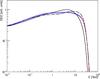 |
Fig. A.1 Electromagnetic cascade spectra in the universal regime for the case of z = 0.02. Solid black – γ-ray, 100 TeV; dashed black – electron, E = 100 TeV; solid red – γ-ray, E = 1 PeV; crosses blue – electron, E = 1 PeV. |
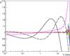 |
Fig. A.3 Ratio of the spectra to the spectrum of primary γ-ray with energy 1 PeV for the case of z = 0.02. Solid black – primary γ-ray, 100 TeV; dashed black – electron, E = 100 TeV; solid red – γ-ray, E = 1 PeV; dashed red – electron, E = 1 PeV; solid green – γ-ray, E = 10 PeV; solid blue – γ-ray, E = 100 PeV; magenta – γ-ray, E = 1 EeV. |
Appendix B: Absorbed and cascade components for various primary spectra of γ-rays
In Fig. B.1 we present several other examples of calculations for the case of a purely electromagnetic cascade and the following primary spectrum: 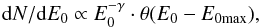 (B.1)
(B.1)
where θ(E0−E0max)= 1 if E0<E0max and 0 otherwise. Figure B.1 top-left, the graph is drawn for the case of γ = 1 and E0max = 100 TeV; Fig. B.1 top-right – for γ = 2 and E0max = 100 TeV, Fig. B.1 middle-left – γ = 3 and E0max = 100 TeV; Fig. B.1 middle-right – γ = 2 and E0max = 10 TeV; Fig. B.1 bottom-left – for γ = 3 and E0max = 10 TeV; Fig. B.1 bottom-right – for γ = 2 and E0max = 1 TeV.
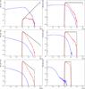 |
Fig. B.1 Primary and secondary components (observable spectrum) of γ-rays from primary γ-rays with power-law shape and different parameters. Black line – primary spectrum in the source, red lines – absorbed and redshifted primary component, blue lines – cascade component. Bars denote statistical fluctuations. |
Appendix C: Optical depth τ in the ELMAG code
Figure C.1 shows the comparison between several models of optical depth τ with the version of the KD10 EBL
model as implemented in the ELMAG code. Other EBL models include G12, KD10 (original implementation) and F08.
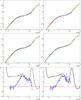 |
Fig. C.1 Comparison of τ vs. energy for G12 (black), F08 (green), KD10 (red), ELMAG KD10 (blue) models for z = 0.129 (top left figure), z = 0.14 (top right figure), z = 0.186 (middle left figure), z = 0.287 (middle right figure) and ratios of G12 and ELMAG KD10 to KD10 (bottom left figure: solid lines for z = 0.129, dashed – for z = 0.14, bottom right figure: solid lines for z = 0.186, dashed – for z = 0.287). |
Appendix D: Comparison of observable γ-ray spectra with other studies
Here we present the comparison of our test calculations with other works. Figure D.1 shows good agreement between our calculations with the ELMAG code, assuming the KD10 EBL model as implemented in ELMAG, and the result of Vovk et al. (2012), obtained with the F08 EBL model. Figure D.2 presents the comparison of our result for the case of the basic hadronic cascade model with the ones obtained by Essey et al. (2011) and Murase et al. (2012).
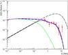 |
Fig. D.1 Comparison of our calculations with the ELMAG code and the result of Vovk et al. (2012) for z = 0.14. Magenta line denotes the total observable spectrum calculated by Vovk et al. (2012) and other lines denote our results: dashed black line – primary spectrum in the source, solid black line – absorbed primary component, solid green line – cascade component, dashed thick blue line – total model spectrum. |
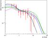 |
Fig. D.2 Comparison between the hadronic model from our work (black-dashed curve, power-law spectrum from 1 EeV to 100 EeV, γ = −2) with other works (solid curves). Black – Essey et al. (2011), high EBL intensity; magenta – Essey et al. (2011), low EBL intensity; green – Murase et al. (2012), KD10 EBL; blue – Murase et al. (2012), Kneiske et al. (2004) best-fit EBL. |
All Tables
All Figures
|
Fig. 1 Primary and secondary components (observable spectra) of γ-rays from primary monoenergetic injection. Black circles – primary energies E0= 1 TeV, red – 3 TeV, green – 10 TeV, blue – 30 TeV, cyan – 100 TeV, and magenta – 1000 TeV= 1 PeV. |
| In the text | |
|
Fig. 2 Spectra of secondary electrons generated in the pair production process. Black line – Ep0 = 1 EeV, red – 10 EeV, green – 30 EeV, blue – 100 EeV. |
| In the text | |
|
Fig. 3 Secondary γ (solid) and positron (dashed) SEDs for the case of photopion losses. Black lines – Ep0 = 30 EeV, red – 50 EeV, green – 70 EeV (green), blue – 100 EeV. |
| In the text | |
|
Fig. 4 w(z) /w(0) dependence. Black line – Ep0 = 10 EeV, red – 30 EeV, green – 50 EeV, blue – 100 EeV. |
| In the text | |
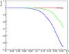 |
Fig. 5 Kem(z) dependence. Meaning of colours is the same as in Fig. 4. |
| In the text | |
|
Fig. 6 Observable γ-ray SED. Dashed magenta line – Ethr= 10 MeV, solid cyan – 10 GeV. Black, red, green, and blue lines denote power-law approximations of the spectrum in various energy regions. |
| In the text | |
|
Fig. 7 Observable SED for various Ep0 (solid curves): black curve – Ep0 = 10 EeV, red – 30 EeV, green – 50 EeV, blue – 100 EeV. SEDs decomposed on the contributions from the primary cascade particles produced at z< 0.06 (dashed curves) and at z> 0.06 (dot-dashed curves) are also shown. |
| In the text | |
|
Fig. 8 The comparison between observable SEDs obtained in the full hybrid approach (circles) and the universal hybrid method approach (solid curves) for different values of the zc parameter: black – zc = 0, red – zc = 0.02, green – zc = 0.05, blue – zc = 0.10, cyan – zc = 0.15, magenta – zc = 0.18. Primary proton energy Ep0 = 30 EeV. The universal spectrum for the case of primary γ-rays with energy 1 PeV is shown for comparison (dashed black line). Relative normalization of all spectra is done at E = 10 GeV. |
| In the text | |
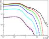 |
Fig. 9 Same as in Fig. 8, but without relative normalization of spectra with different zc. |
| In the text | |
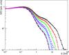 |
Fig. 10 Same as in Fig. 8, but for Ep0 = 100 EeV. |
| In the text | |
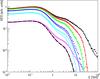 |
Fig. 11 Same as in Fig. 10, but without relative normalization of spectra with different zc. |
| In the text | |
|
Fig. 12 Model fits for the case of 1ES 0347-121. Red circles denote measurements, bars – their uncertainties; long-dashed lines – primary γ-ray spectra. Top-left – absorption-only model: black – G12 EBL model, green – F08, blue – KD10 model as implemented in ELMAG; solid lines – observable spectra. Top-right – electromagnetic cascade model: blue solid line denotes observable spectrum, black – absorbed component, green – cascade component. Middle-left: the same as for top-right, but showing the high-energy cutoff of the primary spectrum. Middle-right – basic hadronic model: black solid line denotes zc = 0, magenta – zc = 0.02, green – zc = 0.05, blue – zc = 0.10; short-dashed line – power-law spectrum of primary protons with zc = 0. Bottom-left – modified hadronic model, the same meaning of colours as in the middle-left panel. Bottom-right – another fit for the case of modified hadronic model. |
| In the text | |
|
Fig. 13 Flux boost factor KB(E) for 1ES 0347-121 (red curve). Blue circles – KB(E) averaged over energy intervals to suppress statistical fluctuations. |
| In the text | |
|
Fig. 14 Model fits for the case of 1ES 0229+200. Top-left – absorption-only model, all notions are the same as in Fig. 11, top-left. Top-right – comparison of the absorption-only and γ-ALP mixing models: black line denotes absorption-only model, green – weak γ-ALP flux enhancement, blue – strong γ-ALP flux enhancement. Middle panels – electromagnetic cascade model for the case of the VERITAS (left) and H.E.S.S. (right, red triangles) observations together with cascade spectra for monoenergetic primary γ-ray injection (short-dashed lines): red – Eγ0 = 10 TeV, blue – Eγ0 = 100 TeV, magenta – Eγ0 = 1 PeV. Bottom-left – basic hadronic cascade model (zc are the same as in Fig. 12 middle-right); bottom-right – modified CR beam model. |
| In the text | |
|
Fig. 15 Fits to the spectrum of 1ES 0229+200 for the electromagnetic cascade model and different values of KV. Dashed lines denote a primary spectrum near the source, solid lines – total model spectra; black – KV= 1, green – 0.6, blue – 0.4, cyan – 0.3, magenta – 0.2. |
| In the text | |
|
Fig. 16 Boost factor KB vs. energy for the fits presented in Fig. 13. Solid lines denote KB(E) for different values of KV: black – KV = 1, green – 0.6, blue – 0.4, cyan – 0.3, magenta – 0.2. Dashed vertical lines denote the energy corresponding to τ = 1: black for the G12 EBL model, red – KD10, green – F08, blue – KD10 as implemented in the ELMAG code. Solid vertical lines denote the energy corresponding to τ = 2 (the same meaning of colours as for dashed vertical lines). |
| In the text | |
|
Fig. 17 Model fits for the case of 1ES 1101-232. Top – the absorption-only model (left) and the electromagnetic cascade model for the case of 2007 reanalysis (right); all notions are as in corresponding panels of Fig. 10. Middle-left – electromagnetic cascade model for the case of 2006 analysis. Middle-right – basic hadronic cascade model in which zc are the same as in Fig. 10 middle-right. Bottom-left and bottom-right – modifed hadronic model (details in the text). |
| In the text | |
|
Fig. 18 Model fits for the case of 1ES 1218+304 (first row, left – absorption-only model; first row, right – electromagnetic cascade model; second row, left – basic hadronic model (black curve – zc = 0, blue curve – zc = 0.15); second row, right – modified hadronic model) and 1ES 0414+009 (third row, left – absorption-only model; third row, right – electromagnetic cascade model; bottom-left – basic hadronic model (black curve – zc = 0, blue curve – zc = 0.25); bottom-right – modified hadronic model). |
| In the text | |
|
Fig. 19 Model fits for the case of H 1426+428. Top-left – absorption-only model, top-right – electromagnetic cascade model (formal best fit). Middle panels – two fits for the electromagnetic cascade model with large contribution of cascade component at low energy. Bottom-left – basic hadronic model (black curve denotes zc = 0, blue curve – zc = 0.1), bottom-right – modified hadronic model. |
| In the text | |
|
Fig. 20 Modification factor KM for different values of B0. Black curve denotes B0 = 1 nG, red curve – 10 nG, green – 100 nG, blue – 1 mkG, magenta – 10 mkG. |
| In the text | |
|
Fig. 21 Model spectrum for different values of B0. Colours denote the same values of B0 as in Fig. 20. |
| In the text | |
|
Fig. 22 Significance (Z-value) of the intermediate hadronic model exclusion for Γ = 10 and blazar emission parameters from T14. |
| In the text | |
 |
Fig. 23 Same as in Fig. 22, but for Γ = 30. |
| In the text | |
|
Fig. A.1 Electromagnetic cascade spectra in the universal regime for the case of z = 0.02. Solid black – γ-ray, 100 TeV; dashed black – electron, E = 100 TeV; solid red – γ-ray, E = 1 PeV; crosses blue – electron, E = 1 PeV. |
| In the text | |
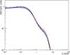 |
Fig. A.2 Same as in Fig. A.1, but for z = 0.186. |
| In the text | |
|
Fig. A.3 Ratio of the spectra to the spectrum of primary γ-ray with energy 1 PeV for the case of z = 0.02. Solid black – primary γ-ray, 100 TeV; dashed black – electron, E = 100 TeV; solid red – γ-ray, E = 1 PeV; dashed red – electron, E = 1 PeV; solid green – γ-ray, E = 10 PeV; solid blue – γ-ray, E = 100 PeV; magenta – γ-ray, E = 1 EeV. |
| In the text | |
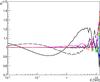 |
Fig. A.4 Same as in Fig. A.3, but for z = 0.186. |
| In the text | |
|
Fig. B.1 Primary and secondary components (observable spectrum) of γ-rays from primary γ-rays with power-law shape and different parameters. Black line – primary spectrum in the source, red lines – absorbed and redshifted primary component, blue lines – cascade component. Bars denote statistical fluctuations. |
| In the text | |
|
Fig. C.1 Comparison of τ vs. energy for G12 (black), F08 (green), KD10 (red), ELMAG KD10 (blue) models for z = 0.129 (top left figure), z = 0.14 (top right figure), z = 0.186 (middle left figure), z = 0.287 (middle right figure) and ratios of G12 and ELMAG KD10 to KD10 (bottom left figure: solid lines for z = 0.129, dashed – for z = 0.14, bottom right figure: solid lines for z = 0.186, dashed – for z = 0.287). |
| In the text | |
|
Fig. D.1 Comparison of our calculations with the ELMAG code and the result of Vovk et al. (2012) for z = 0.14. Magenta line denotes the total observable spectrum calculated by Vovk et al. (2012) and other lines denote our results: dashed black line – primary spectrum in the source, solid black line – absorbed primary component, solid green line – cascade component, dashed thick blue line – total model spectrum. |
| In the text | |
|
Fig. D.2 Comparison between the hadronic model from our work (black-dashed curve, power-law spectrum from 1 EeV to 100 EeV, γ = −2) with other works (solid curves). Black – Essey et al. (2011), high EBL intensity; magenta – Essey et al. (2011), low EBL intensity; green – Murase et al. (2012), KD10 EBL; blue – Murase et al. (2012), Kneiske et al. (2004) best-fit EBL. |
| In the text | |
Current usage metrics show cumulative count of Article Views (full-text article views including HTML views, PDF and ePub downloads, according to the available data) and Abstracts Views on Vision4Press platform.
Data correspond to usage on the plateform after 2015. The current usage metrics is available 48-96 hours after online publication and is updated daily on week days.
Initial download of the metrics may take a while.