| Issue |
A&A
Volume 602, June 2017
|
|
|---|---|---|
| Article Number | A25 | |
| Number of page(s) | 22 | |
| Section | Astrophysical processes | |
| DOI | https://doi.org/10.1051/0004-6361/201629997 | |
| Published online | 30 May 2017 | |
Expected signatures from hadronic emission processes in the TeV spectra of BL Lacertae objects
1 LUTH, Observatoire de Paris, CNRS, Université Paris Diderot, PSL Research University, 5 place Jules Janssen, 92190 Meudon, France
e-mail: This email address is being protected from spambots. You need JavaScript enabled to view it.
2 LPNHE, Université Pierre et Marie Curie Paris 6, Université Denis Diderot Paris 7, CNRS/IN2P3, 4 place Jussieu, 75252 Paris Cedex 5, France
e-mail: This email address is being protected from spambots. You need JavaScript enabled to view it.
3 Institute for Cosmic Ray Research, University of Tokyo, Tokyo 113-8654, Japan
Received: 2 November 2016
Accepted: 16 February 2017
Abstract
Context. The wealth of recent data from Imaging Air Cherenkov telescopes (IACTs), ultra-high energy cosmic-ray experiments and neutrino telescopes have fuelled a renewed interest in hadronic emission models for γ-loud blazars.
Aims. We explore physically plausible solutions for a lepto-hadronic interpretation of the stationary emission from high-frequency peaked BL Lac objects (HBLs). The modelled spectral energy distributions are then searched for specific signatures at very high energies that could help to distinguish the hadronic origin of the emission from a standard leptonic scenario.
Methods. By introducing a few basic constraints on parameters of the model, such as assuming the co-acceleration of electrons and protons, we significantly reduced the number of free parameters. We then systematically explored the parameter space of the size of the emission region and its magnetic field for two bright γ-loud HBLs, PKS 2155-304 and Mrk 421. For all solutions close to equipartition between the energy densities of protons and of the magnetic field, and with acceptable jet power and light-crossing timescales, we inspected the spectral hardening in the multi-TeV domain from proton-photon induced cascades and muon-synchrotron emission inside the source. Very-high-energy spectra simulated with the available instrument functions from the future Cherenkov Telescope Array (CTA) were evaluated for detectable features as a function of exposure time, source redshift, and flux level.
Results. A range of hadronic scenarios are found to provide satisfactory solutions for the broad band emission of the sources under study. The TeV spectrum can be dominated either by proton-synchrotron emission or by muon-synchrotron emission. The solutions for HBLs cover a parameter space that is distinct from the one found for the most extreme BL Lac objects in an earlier study. Over a large range of model parameters, the spectral hardening due to internal synchrotron-pair cascades, the “cascade bump”, should be detectable for acceptable exposure times with the future CTA for a few nearby and bright HBLs.
Key words: radiation mechanisms: non-thermal / astroparticle physics / radiative transfer / gamma rays: galaxies / BL Lacertae objects: individual: PKS 2155-304 / BL Lacertae objects: individual: Mrk 421
© ESO, 2017
1. Introduction
The still-open question on the origin of ultra-high-energy cosmic rays (UHECRs) and astrophysical neutrinos on the one hand, and the wealth of available data from γ-ray emitting blazars on the other (from MeV to TeV energies, see e.g. Ackermann et al. 2011; Senturk et al. 2013), has led to renewed interest in hadronic emission models for those sources. Radiative emission in the most common scenarios either comes from a region inside the relativistic jet (e.g. Mannheim 1993; Dermer & Atoyan 2001; Mücke & Protheroe 2001; Dimitrakoudis et al. 2012; Bosch-Ramon et al. 2012; Böttcher et al. 2013; Mastichiadis et al. 2013; Petropoulou et al. 2015; Diltz et al. 2015 or from interactions of escaping hadrons along the path from the source to Earth (e.g. Essey & Kusenko 2010; Essey et al. 2011; Dermer et al. 2012; Murase et al. 2012; Tavecchio 2014). Contrary to the more commonly assumed leptonic scenarios, in which the two characteristic broad bumps of the non-thermal spectral energy distribution (SED) of blazars are described with electron-synchrotron and Inverse Compton emission (Konigl 1981; Sikora et al. 1994), hadronic scenarios introduce relativistic protons to explain the high-energy bump that is generally seen from keV to GeV energies in flat-spectrum radio quasars (FSRQs) and in the MeV to TeV range for BL Lac objects. In the hadronic framework, this high-energy component can be attributed to either proton-synchrotron emission or radiation from secondary products of proton-photon or proton-proton interactions. These kinds of scenarios thus admit the possibility of a direct link between UHECRs and electromagnetic emission from blazars. They also lead necessarily to the emission of high-energy neutrinos from the decay of proton-induced pions and muons. This suggests that blazars, or more generally radio-loud active galactic nuclei (AGNs), of which blazars are a sub-class of objects with their jets assumed to be closely aligned to the line of sight, are potential sources of the PeV neutrinos recently detected with IceCube (Aartsen et al. 2013).
Even though hadronic emission models in general require higher jet powers and face more difficulties to account for short-term variability than leptonic models, they still present a viable and very intriguing alternative within the available constraints from current observational data. Future instruments, such as the Cherenkov Telescope Array (CTA; Actis et al. 2011; Acharya et al. 2013), will be able to probe blazar spectra above a few tens of GeV and cover the whole very-high-energy range (VHE, energies above 100 GeV) to above 100 TeV, with much better sensitivity and spectral resolution than current Imaging Air Cherenkov telescopes (IACTs). This motivates a search for potential signatures in the VHE γ-ray spectrum that would help distinguish hadronic scenarios from the simpler leptonic models.
Cerruti et al. (2015, hereafter C15 have recently characterised the SEDs of a distinct class of so-called ultra-high-frequency peaked BL Lac objects (UHBLs) with a stationary one-zone model that provides a complete treatment of all relevant emission processes for relativistic electrons and protons. This model, which will also be used for the current study, allows us to treat leptonic, hadronic and mixed scenarios with a single code. The authors have shown that hadronic and mixed lepto-hadronic scenarios provide an interesting alternative for the interpretation of UHBL SEDs, compared to purely leptonic synchrotron self-Compton (SSC) models. The latter are found to require extreme parameters for such sources. Two distinct regions were identified in the parameter space spanned by the source extension and magnetic field strength, leading to interpretations of the high-energy bump either as proton-synchrotron dominated (“hadronic” solution; for high magnetic fields of the order of a few 10 G) or as consisting of a combination of SSC radiation and emission from synchrotron-pair cascades triggered by proton-photon interactions and the subsequent decay of the generated pions and other mesons (mixed “lepto-hadronic” solution; for magnetic fields of the order of a few 0.1 G). In each of these parameter regions, solutions were found with jet powers below the Eddington luminosity, distinguishing these objects from the more luminuous blazar classes studied by Zdziarski & Böttcher (2015), which require very high jet powers.
Although UHBLs are located at the most extreme end of the “blazar sequence” (Fossati et al. 1998), high-frequency peaked BL Lac objects (HBLs) with a high-energy peak located in the 0.1 to 1 TeV range are far more numerous in the current sample of blazars detected with IACTs. They clearly outnumber all other types of blazars detected at these energies1. Hadronic solutions are routinely proposed as alternatives to the standard SSC scenario for these kinds of sources, but a systematic exploration of (lepto-)hadronic solutions for a given dataset has not yet been attempted, to the best of our knowledge. A more general study of the impact of the magnetic field strength and density of the target photon field of the proton-synchrotron model is presented by Mücke et al. (2003). In most of the current literature, very few a priori physical constraints are imposed and only exemplary solutions are presented.
After a short description of the physical constraints we impose on our model to reduce the number of free parameters (Sect. 2), we explore the characteristics of different hadronic solutions for HBLs with respect to the source extension, magnetic field strength, jet power, and equipartition between the magnetic and kinetic energy density in Sect. 3. Then we apply the model to SEDs of the two HBLs PKS 2155-304 and Mrk 421 from low flux states in Sect. 4. We describe the different sets of solutions, and briefly discuss the jet power, deviation from equipartition and variability timescales they imply. In Sect. 5, we compare these solutions to a previous study of UHBLs. We then search the modelled SEDs for signatures of spectral hardening in the VHE range, which are caused by the emission from synchrotron-pair cascades and from muon-synchrotron radiation, and compare these to the expected sensitivity of CTA in Sect. 6. The relation of the detectability of such features to the flux level and redshift are explored. Finally, we present a critical discussion of these results, their limitations, and implications for UHECR and astro-neutrino searches in Sect. 7.
Throughout this work, the absorption on the extragalactic background light (EBL) is computed using the model by Franceschini et al. (2008). In Sect. 7, we discuss how this particular choice affects our results. For the transformations between the two nearby blazars under study and the observer on Earth, we have adopted a standard cosmology with Ωm = 0.3, ΩΛ = 0.7, and H0 = 68 km s-1 Mpc-1.
2. Physical constraints of model parameters
LEHA (see C15) is a code that was developed recently to simulate the stationary emission from BL Lac objects for leptonic, hadronic, and mixed scenarios. In this “blob in jet” code, relativistic populations of electrons and protons are confined within a plasma blob of radius R with a tangled magnetic field of strength B and a bulk Lorentz factor Γ. The primary particle distributions follow power laws with self-consistent synchrotron cooling breaks.
In addition to synchrotron emission from primary protons and electrons, and SSC emission, the code also treats proton-photon interactions with meson-production and subsequent decay by use of the SOPHIA Monte Carlo package (Mücke et al. 2000). Secondary particles from such interactions trigger pair-synchrotron cascades that are followed for several generations. In addition, the muon-synchrotron spectrum is extracted following slight modifications of the SOPHIA code. In the LEHA code, Bethe-Heitler and photon-photon pair production are calculated and the synchrotron-pair cascades they trigger are evaluated as well. Only proton-proton interactions are not considered, because to be efficient this kind of a process would require very high target proton densities inside the jet in our framework.
In our application to high-frequency peaked BL Lac objects, the code provides a simple description for a continuous plasma flow through a stationary or slowly-moving acceleration region inside the jet, without specification of the acceleration mechanism. A flow of accelerated particles is continuously injected into a stationary or slowly moving radiation zone and then continues down the jet with bulk Lorentz factor Γ, while expanding adiabatically. This picture is motivated by the fact that very long baseline interferometry (VLBI) observations of a large sample of blazars show that although luminous blazar types often exhibit rapidly-moving radio knots, in HBLs they tend to be stationary (e.g. Hervet et al. 2016). The homogeneous, spherical emission zone of constant radius that we are modelling represents the radiation region into which particles are injected. Radiative emission is strongly dominated by emission from this zone, because the plasma flow rapidly loses energy through adiabatic expansion farther down the jet. For example, when imposing that the magnetic flux be conserved, the magnetic field strength scales as B ∝ R-2, implying an energy output through synchrotron emission that is proportional to R-4. The decreasing particle density (proportional to R-3) together with the decreasing target photon density also leads to a rapid reduction in the proton-photon interaction rate. In addition, radiative losses will further reduce the emission level, especially at the highest energies where our study is focused. Therefore only the single acceleration and emission zone is modelled and emission from the plasma flow farther down the jet is neglected.
To reduce the number of free parameters and to focus on physically plausible solutions from the onset, we impose a number of constraints that are based on simplifying assumptions about the nature of the emission region and the acceleration process. These constraints correspond for the most part to those applied by C15:
-
Leptons and protons are supposed to be co-accelerated and tofollow power laws with the same intrinsic index n1, before cooling. This index is assumed to be close to two, consistent with Fermi-like acceleration mechanisms. However, no specific assumptions are made about the underlying mechanism.
-
To account for synchrotron cooling of the primary particles, the stationary spectra of primary electrons and protons, which are used as an input to the code, are characterised by broken power laws with exponential cut-offs (see C15, Eq. (1)). The Lorentz factors corresponding to the break energies γ(e;p),break are determined from a comparison of radiative and adiabatic cooling timescales. The second spectral slope above these breaks is given by n2 = n1 + 1. For the application to HBLs, the electron population is generally completely cooled, whereas the proton spectrum is not impacted. We verify that for all the solutions presented here, proton energy loss is indeed always dominated by adiabatic cooling and thus there is no cooling break in the proton spectra. Comparisons of the relevant acceleration and cooling timescales for a few exemplary models are shown in Appendices C and D and are discussed below.
-
The minimum proton Lorentz factor γp,min is not constrained and is set to one, whereas for the electron spectrum we generally need to adjust the minimum Lorentz factor γe,min to match constraints from low-energy optical and radio data. This choice for γp;min maximises the proton energy density up, which represents a major contribution to the jet power. It is thus a conservative choice when considering the energetics of the models.
-
The maximum proton Lorentz factor γp;max, is derived from the equilibrium between particle acceleration and energy loss, meaning radiative and adiabatic cooling, through a comparison of their characteristic timescales. The acceleration timescale as a function of the Lorentz factor is simply described by τacc(γ) = γ/ψ·mc/ (eB) with an assumed efficiency of ψ = 0.1. In the regime where adiabatic cooling dominates over radiative cooling, which is the regime of interest for HBLs in our framework, the maximum proton Lorentz factor is
 (1)as can be seen from Eq. (18) in C15. The same behaviour is found when simply applying the Hillas criterion (Hillas 1984) to constrain γp;max. The maximum energy of the electron spectrum, defined by the Lorentz factor γe,max, is left as a free parameter that we constrain with X-ray data. For the solutions found here, the ratio of γp,max over γe,max is consistent with the values one might expect in diffusive acceleration for a Kraichnan turbulence spectrum, but a specific investigation of the acceleration mechanism is beyond the scope of the present work (cf. Biermann & Strittmatter 1987; Mücke & Protheroe 2001; and C15 for more discussion).
 -
The bulk Doppler factor of the emission region is fixed at δ = 30, a typical value for bright VHE-detected BL Lac objects (Tavecchio et al. 2010). This allows for the observed variability in those sources when using reasonable source parameters, except for the most extreme minute-scale flares (Gaidos et al. 1996; Aharonian et al. 2007; Albert et al. 2007), the origin of which are not yet clearly understood. The impact on our study of the value of this parameter is discussed briefly in Sect. 7.
-
We also assume that the viewing angle between the jet axis and the line of sight to the observer is very small, leading to a relation between bulk Doppler factor and bulk Lorentz factor of
 (2)This small-angle approximation seems justified when considering that we are investigating particularly bright sources in this study.
Given these constraints, we are left with: two quantities, B and R, that we treat as free parameters; and five quantities, n1, γe,min, γe,max, and the normalisation of the electron and proton spectra K(e;p), that are more or less constrained by the SED for a given choice of the free parameters. To find a complete set of solutions for a given source, we first varied n1 for values close to two that provided a satisfactory representation of the optical and X-ray data. Then, for a small set of the selected n1 values, we scanned B and R while adjusting the particle densities for electrons and protons with K(e;p), and the minimum and maximum electron energies to the SED, using the usual “fit-by-eye” method. The flux level of the electron- and proton-synchrotron peaks in the SED can be kept constant during these scans by varying the particle densities as  (3)where the last term is a function of the maximum particle Lorentz factor, the Lorentz factors of the cooling breaks, and the spectral index of the particle distributions, which all influence the particle content of the source.
We also constrained the parameter space of models for a given SED by requiring that the size of the emission region and the overall jet power be physically acceptable. A characteristic size scale for AGNs is given by the Schwarzschild radius RS of the supermassive black hole. Although for blob-in-jet models one generally expects emission regions of a size at least an order of magnitude larger than the Schwarzschild radius, as a minimum requirement we discarded only those solutions with R<RS. The maximum size of the emission region is usually limited by comparing the light-crossing time to the observed variability timescale of the source, but for the persistent flux states we are interested in, the latter information is generally not available or not very constraining. This will be discussed more in Sect. 7.
The jet power for a two-sided jet was estimated as  (4)where uB, ue, up are the co-moving stationary energy densities of the magnetic field, electrons and protons, respectively, and Lr corresponds to the power in the radiation field (e.g. Dermer et al. 2014, and references therein). In hadronic scenarios, ue and Lr are generally very small compared to the other components and thus we neglected them. Any additional component due to cold protons inside the jet were also neglected. As is usually the case in one-zone hadronic scenarios, the jet power was assumed to be largely dominated by the power from the “blob”. An additional extensive jet could have been added, as is done for certain leptonic models (see e.g. Katarzyński et al. 2001; Abramowski et al. 2012; Hervet et al. 2015) if one wants to account for electron synchrotron emission in the radio band, but its contribution to the total jet power would be much smaller than that from the “blob”.
The value of Lj is not constrained from first principles, but can be compared to the Eddington luminosity Ledd as an order-of-magnitude reference. Based on measurements of the jet power of radio-loud AGNs from X-ray cavity data (e.g. Cavagnolo et al. 2010), highly super-Eddington powers are generally not expected. We conservatively required that acceptable solutions should have Lj<Ledd for a given source.
We also derived the ratio η between the kinetic energy density of the relativistic particles, which is largely dominated by up for all our solutions, and the energy density of the magnetic field uB:  (5)Solutions can then be characterised by their proximity to equipartition between these components (η = 1). For stationary solutions, having a system close to equipartition is physically appealing (e.g. discussion by Böttcher et al. 2013) and models close to equipartition are in general also energetically favoured, such that η can be used as an order-of-magnitude reference to select physically plausible solutions. We required 0.1 <η< 10 in the following. It should however be noted that deviation from equipartition between kinetic electron-energy density and magnetic energy density, even by more than an order of magnitude, is frequently encountered in the standard one-zone SSC models for these type of sources (e.g. Cerruti et al. 2013).
3. Hadronic scenarios for high-frequency peaked BL Lac objects
When modelling the SEDs of high-frequency peaked BL Lac objects within our hadronic scenario, we distinguish two limiting cases. These depend on whether the VHE spectrum is dominated by proton-synchrotron emission from the primary protons or by muon-synchrotron emission from muons generated in pion decays that follow proton-photon interactions. In general, both components contribute at least to some extent to the VHE spectrum. In all the hadronic scenarios discussed here, the low-energy bump of the SED that covers the optical to X-ray range is interpreted as electron-synchrotron radiation2.
3.1. Proton-synchrotron dominated very-high-energy spectrum
In this scenario, proton-synchrotron emission is responsible for the entire high-energy bump. A contribution from muon-synchrotron or cascade emission only appears above several TeV or tens of TeV, where it can lead to small spectral features as will be discussed below. When the high-energy bump is ascribed to proton-synchrotron emission, the proton-synchrotron peak frequency is fixed to the peak frequency of the bump.
Solutions with a constant synchrotron peak frequency lie on diagonal lines in the log B-log R parameter plane that satisfy  (6)for a given n1 and δ. This can be seen from Eqs. (20) and (29) in C15. Solutions with higher or lower peak frequencies lie on parallels towards higher or lower values of R, respectively. This is shown schematically in Fig. 1. All the solutions for the HBLs we have studied lie in the adiabatic cooling dominated regime, meaning to the left of the bold line in Fig. 1.
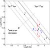 |
Fig. 1 Location of hadronic solutions in the log R-log B parameter plane. The frequency of the proton synchrotron emission peak remains constant along the dashed lines. The solid diagonal line separates the adiabatic cooling dominated domain from the radiative cooling dominated domain. The location of the typical solutions for HBLs shown in Figs. 2, 4 and 5 are indicated with markers and numbers. The dotted arrow points in the direction of decreasing proton synchrotron peak frequency. |
 |
Fig. 2 Variation in the modelled SED when moving along the diagonal in log R-log B space. From left to right, models with log B [G] = 0.5, 1.5, 2.0 are shown. Particle densities are adjusted to maintain the same overall flux level between the different models. Solid red and blue lines indicate the electron and proton synchrotron emission. The dotted and dashed lines show muon-synchrotron emission at the highest energies, and the SSC and muon-synchrotron cascade components at lower energies, as indicated in the legend. The VHE spectrum is absorbed by the EBL, assuming a redshift of 0.116, corresponding to the source PKS 2155-304. The spectral index n1 is chosen to be 1.9. The two dashed vertical lines are there to guide the eye by marking the approximate peak postitions of the model in the central figure. |
When moving along the diagonal line of constant peak frequency towards higher B and smaller R while keeping the flux level constant, the equipartition ratio η increases. The magnetic energy density uB increases as B2. The proton energy density up increases roughly as B3 due to the relation given in Eq. (6)and the dependence of γp,max on R and B (cf. Eq. (1)). As η increases, proton-photon interactions become more frequent, leading to a more significant contribution from subsequent synchrotron-pair cascades and from muon-synchrotron emission. This can be seen in Fig. 2, in which model SEDs are shown for three different locations on a diagonal in the log B-log R plane. The proton-synchrotron component remains dominant as long as the peak frequency is sufficiently high and the particle density remains sufficiently low. This is particularly the case for all the hadronic solutions found for UHBLs, as will be discussed in Sect. 5.
Increasing B moves the low energy cut-off in the electron-synchrotron spectrum to higher frequencies, as shown in Fig. 2, whereas solutions with large R and small B require large γe;min, so as not to violate constraints from optical and radio data. Very large values of γe;min are however physically difficult to account for, except in very specific scenarios (see for example the discussion by Katarzyński et al. 2006).
From Eqs. (4)and (6)it can be seen that the jet power decreases with 1 /B when moving on the diagonal towards higher B and lower R, as long as the contribution from the magnetic energy density dominates, meaning η ≪ 1. Once the proton energy density dominates, Lj remains approximately constant for n1 ~ 2. The location of the different solutions in the log Lj-log η plane is shown in Fig. 3.
 |
Fig. 3 Location of hadronic solutions in log Lj-log η parameter space. The markers indicated the same solutions as shown in Fig. 1. The dashed curve represents the location of the proton-synchrotron solutions for a higher spectral index of the particle population. The vertical line marks equipartition between energy density of the magnetic field and relativistic protons. |
In the same figure, a second set of solutions is given for a different, larger value of n1. When increasing n1 for a given B and R, the proton energy density up increases because a given population of protons close to γp;max implies a larger population of protons at lower energy. This also leads to an increase in Lj and η.
3.2. Muon-synchrotron dominated very-high-energy spectrum
Starting from a given proton-synchroton dominated solution, one can find an alternative scenario when moving to lower values of B or R (cf. Fig. 1, red and blue lines) or both. This will shift the proton-synchrotron peak to a lower frequency, but will also lead to an increase of η, due to an increase in particle density that compensates the smaller emission region or magnetic field strength. In the modelled SED, this results in a stronger presence of emission from cascades and from the muon-synchrotron component at high energies. In this scenario, the high-energy bump is thus represented by a combination of different proton-induced components.
An example for the transition from a proton-synchrotron to a muon-synchrotron dominated VHE spectrum is shown in Figs. 4 and 5. The muon-synchrotron and cascade emission becomes dominant in the TeV range in Fig. 4 in the right panel. Variations in either R or B lead to very similar models, except that by decreasing only B one lowers the energy cut-off in the electron-synchrotron spectrum. Note the small shift in the left slope of the low-energy bump in Fig. 5 between the three panels.
 |
Fig. 4 Variation in the modelled SED when varying R, i.e. moving along the red line in log R-log B space. From left to right, models with log R [cm] = 15.7, 15.3, and 15.0 are shown. Particle densities are adjusted to maintain the same overall flux level between the different models. Definition of the different curves as in Fig. 2. |
 |
Fig. 5 Variation in the modelled SED when varying B, i.e. moving along the blue line in log R-log B space. From left to right, models with log B [G] = 1.7, 1.5, 1.3 are shown. Particle densities are adjusted to maintain the same overall flux level between the different models. Definition of the different curves as in Fig. 2. |
When lowering B or R from a given initial value while keeping the flux level constant, the jet power Lj decreases as long as uB dominates over up. As η increases, up will eventually become dominant and Lj will increase, as can be derived from Eq. (4). The muon-synchrotron dominated scenario provides an energetic advantage for another reason: due to the combination of several components in the high-energy bump, the spectral index n1 is no longer constrained by the often relatively flat high-energy spectrum in the MeV and GeV range, in the νFν representation. This scenario can accommodate broad high-energy bumps with smaller n1 than the proton-synchrotron scenario, leading to a lower Lj due to the smaller proton number density.
3.3. Appearance of a “cascade bump” spectral feature
The combination of spectral components from proton-synchrotron emission and from proton-photon interactions can lead to spectral hardening in the VHE spectrum, as is seen in some of the exemplary models in Figs. 2, 4, and 5. The necessary condition for this kind of a feature to occur is a sufficiently high value of η, such that proton-photon interactions are non-negligible against proton-synchrotron emission. For the proton-synchrotron scenario this is the case for solutions on the diagonal towards large B and small R, where the muon-synchrotron component starts becoming visible at the highest energies.
This “cascade bump” feature can also be seen in certain muon-synchrotron solutions. When the muon-synchrotron component is very prominent, the transition between muon and proton synchrotron emission occurs below the TeV spectrum and could lead to distinctive features between the Fermi-LAT and TeV energy ranges. In other cases, both the proton and muon-synchrotron emission contribute to the TeV spectrum, which can lead to spectral features from the muon and cascade emission at the highest observable energies. It should be mentioned that this feature is also seen in other hadronic models (e.g. Mücke et al. 2003; Böttcher et al. 2013), but there has been no systematic study of its dependence on the model parameters and of its detectability. Because this feature depends on the relative contributions from several components and thus on the exact parameter set used for a given solution, the only feasible approach to evaluate its prevalence seems to be a case study of a large number of solutions for a few given sources, which is attempted in the following section.
4. Application to PKS 2155-304 and Mrk 421
4.1. Datasets and constraints
We selected two prominent TeV emitting HBLs as exemplary sources for our study, because their broad-band SEDs have been well measured in several multi-wavelength campaigns: Mrk 421 in the northern hemisphere and PKS 2155-304 in the southern hemisphere. Because we are interested in the persistent emission from these blazars and do not try to interpret emission from flares, we focus here on datasets corresponding to low flux states.
 |
Fig. 6 SEDs for PKS 2155-304 with two hadronic models where proton synchrotron emission (left figure) or muon-synchrotron emission (right figure) dominates the TeV spectrum. These solutions correspond to a spectral index of n1 = 2.1 and 1.9, a magnetic field with log B [G] = 0.3 and 0.7, and an emission region of size log R [cm] = 9 × 10¹⁶ and 1.5 × 10¹⁶, respectively. See Fig. 2 for a description of the different curves. The dataset is described in the text. |
The nearby blazar Mrk 421 has a redshift of z = 0.031. The black hole at its centre has a mass of about 1.7 × 10⁸M⊙ (Woo et al. 2005), and thus a Schwarzschild radius RS,Mrk421 ~ 5.0 × 1013 cm. This corresponds to an Eddington luminosity of Ledd,Mrk421 ~ 2.1 × 1046 erg s-1.
The SED for Mrk 421 taken from Abdo et al. (2011), from a multi-wavelength campaign in 2009 in which the source was found in a low flux state, includes: data points from several telescopes in the radio and optical band, data from Swift (X-rays and UV), RXTE (X-rays), Fermi-LAT (γ-rays), and MAGIC (VHE). The published MAGIC spectrum had been de-absorbed by the authors using the EBL model by Franceschini et al. (2008). To compare the spectral points with our model curve, we absorbed the published VHE data points using the same model. The high-energy bump of the SED peaks around 100 GeV with a peak energy flux of roughly 8 × 10-11 erg cm-2 s-1.
The HBL PKS 2155-304 is more distant than Mrk 421, with a redshift of z = 0.116. Its black-hole mass is still subject to discussion. Based on measurements of the host-galaxy luminosity by Kotilainen et al. (1998) and on the relations given by Bettoni et al. (2003), a mass of 1−2 × 10⁹M⊙ is estimated by Aharonian et al. (2007). However, when accounting for the scatter in the relation between bulge luminosity and black-hole mass, its mass could be as low as 2 × 10⁸M⊙ (Rieger & Volpe 2010; McLure & Dunlop 2002). In addition, as pointed out by Aharonian et al. (2007), the host galaxy luminosity might require further confirmation. We thus considered a range for the Schwarzschild radius of RS,PKS2155−304 ~ 3 × 10¹³−3 × 1014 cm, corresponding to Ledd,PKS2155−304 ~ 3 × 1046−3 × 1047 erg s-1.
The SED for PKS 2155-304, taken from Aharonian et al. (2009b), includes data from the ATOM telescope (optical), SWIFT, RXTE, Fermi-LAT, and H.E.S.S. (VHE), all taken during a multi-wavelength campaign in 2008, in which PKS 2155-304 was found in a relatively low, although not quiescent state. The published VHE data in this case correspond to the absorbed fluxes. The high-energy bump of the SED peaks around a few 10 GeV, with a peak energy flux of roughly the same level as for Mrk 421.
4.2. Hadronic solutions for PKS 2155-304
When we interpreted the high-energy bump as proton synchrotron emission, the spectral index of the proton population was constrained by the Fermi-LAT spectrum to n1 ≳ 2.0. This also fixed the spectral index of the electron population following our simple co-acceleration scenario. Given the high magnetic field strengths in this scenario, the entire electron population is cooled by synchrotron radiation and has thus a photon index of n1 + 1. The parameters γe;min and γe;max had to be adjusted to obey the constraints from the optical and X-ray emission, which we assumed to stem from the same emission region as the high-energy radiation.
The high-energy bump could also be modelled as a combination of a proton-synchrotron peak in the Fermi-LAT band and a muon-synchrotron component that dominates the TeV spectrum. In this case, the spectral index of the proton spectrum was smaller, meaning that the spectrum was steeper in the high-energy range than in the proton-synchrotron dominated scenario.
We found good solutions for 1.9 ≲ n1 ≲ 2.1. Models with smaller n1 are no longer compatible with the optical and X-ray data, whereas larger n1 provide still acceptable representations of the SED, but lead to very large jet powers Lj>Ledd,PKS2155−304. These solutions correspond to a wide range of magnetic field strengths. For B smaller than a few Gauss, the source extension and jet power become very large. On the other hand, B ≳ 100 G corresponds to solutions with very small R, close to RS,PKS2155−304.
Two examples of such solutions for PKS 2155-304 are shown in Fig. 6. A visible “cascade bump” appears in the VHE spectrum in both cases. The relevant acceleration and cooling timescales of the particle populations for these two solutions are shown in Appendix A. In all cases, energy losses are clearly dominated by adiabatic losses, and photo-meson losses, which are dominated by photopion production, are the slowest processes. Differences between the two solutions for each source are relatively small. The photo-meson time scale is smaller for the solutions with smaller R and higher particle densities. The solutions for Mrk 421 have smaller source extensions, leading to shorter timescales for adiabatic cooling and thus smaller maximum proton energies.
The hadronic solutions for both sources are located inside the adiabatic-cooling dominated regime in log B-log R space (cf. Fig. 7). For PKS 2155-304, solutions can be found over the whole physically acceptable range of source extensions. The contribution from muon-synchrotron and cascade emission is completely negligible for magnetic fields of a few Gauss but increases up to the same level as proton-synchrotron emission at the highest allowed magnetic fields, meaning approximately 100 G.
 |
Fig. 7 Source extension vs. magnetic field for HBL models. The different symbols correspond to the two different sources and to different spectral indices n1. The grey band indicates the range of values suggested for the Schwarzschild radius of PKS 2155-304, whereas the blue line shows the Schwarzschild radius of Mrk 421. |
Large source extensions imply long variability timescales that might pose a problem for sources such as PKS 2155-304 and Mrk 421 that are known for their rapid variability, although rapid flares and the continuous component likely arise from different emission regions (see e.g. Abramowski et al. 2012). It should also be noted that the minimum Lorentz factor for the electron distribution can become large for very extended sources. Although for all the solutions for Mrk 421 that are discussed below γmin does not become larger than about 700, for the PKS 2155-304 models with the largest extensions it can increase up to 1800.
The energy budget of the solutions for PKS 2155-304 can be dominated by the energy density of the protons or of the magnetic field, as seen in Fig. 8. The jet power becomes large for solutions with small magnetic fields and thus large emission regions. As discussed above, the value of n1 has a strong influence on the jet power. For the study presented in Sect. 6, we consider all the solutions shown in Figs. 7 and 8, but the most easily acceptable solutions in terms of jet power and source extension are those with intermediate values of R and B and a relatively small n1.
 |
Fig. 8 Jet power vs. equipartition ratio for HBL models. The different symbols correspond to the two different sources and to different spectral indices n1. The grey band indicates the range of values suggested for the Eddington luminosity of PKS 2155-304, whereas the blue line shows the Eddington luminosity of Mrk 421. |
4.3. Hadronic solutions for Mrk 421
For the SED of Mrk 421, the proton-synchrotron scenario does not provide an acceptable solution because the spectral index n1 is strongly constrained by the optical data, ruling out solutions with a sufficiently flat shape of the high-energy bump to match the Fermi-LAT data. Good solutions are restricted to values of 1.7 ≲ n1 ≲ 1.9 and require a significant contribution from muon-synchrotron emission to reproduce the shape of the high-energy bump. Two examples of such solutions are shown in Fig. 9.
 |
Fig. 9 SEDs for Mrk 421 with two hadronic models where muon-synchrotron emission dominates the TeV spectrum. These solutions correspond to a spectral index n1 = 1.7 and 1.9, a magnetic field with log B [G] = 1.9 and 1.5, respectively, and an emission region of size log R [cm] = 1.5 × 10¹⁴ and 5.7 × 10¹⁴, respectively. See Fig. 2 for a description of the different curves. The dataset is described in the text. |
These solutions occupy a restricted range of magnetic field strengths, as seen in Fig. 7. For B smaller than a few 10 G, the muon-synchrotron component is too low compared to the proton-synchrotron component to match the given flux level, and the proton-synchrotron peak has shifted too far to lower energies, leading to a depression in the TeV spectrum. The hadronic solution proposed by Abdo et al. (2011), using the model by Mücke & Protheroe (2001), which served as an inspiration for the hadronic part of our code, falls into the same region as our solutions with log B [G] = 1.7 and log R [cm] = 14.6, even though their Doppler factor is much smaller with δ = 12.
As is shown in Fig. 8, the solutions are characterised by an energy budget close to equipartition and by a total jet power that is lower than in the case of PKS 2155-304. In fact, all solutions for Mrk 421 have Lj< 0.1Ledd,Mrk421. When comparing solutions with the same magnetic field strength and the same proton index n1 = 1.9 for the two sources, the jet power necessary for the PKS 2155-304 model is about a factor of five larger than for Mrk 421. Given the similar observed flux levels of the two sources, to compensate for the difference in redshift between them a larger emission region and a higher particle density are needed for PKS 2155-304, leading to an increased jet power and a higher maximum proton energy. Although the high-energy bump for these parameters is interpreted as muon-synchrotron emission for Mrk 421, proton-synchrotron radiation dominates in PKS 2155-304.
When comparing our solutions for Mrk 421 to the one proposed by Abdo et al. (2011), the jet powers are very similar, such that log Lj [erg/s] = 44.7 for the latter. However, the smaller δ in their solution requires compensation through a higher proton density and leads to a clear dominance of the proton energy with log (η) = 0.7.
4.4. Synchrotron self-Compton and mixed lepto-hadronic solutions
A standard one-zone SSC model cannot account for the observed SEDs if one assumes that the electron input spectrum is a simple power law that is only modified by a synchrotron cooling break. One-zone SSC solutions require the introduction of an ad hoc broken-power-law shape for the electron distribution, in violation of our physical assumptions.
When loosening those assumptions for electron populations following a broken power law, accurate representations can be found for both SEDs with the exception of the optical data from the ATOM telescope in the SED of PKS 2155-304, which seem to require either an additional component (Abramowski et al. 2012) or a more complicated electron distribution (Aharonian et al. 2009b). When we adjusted the model to the X-ray, γ-ray, and VHE data while constraining the shape of the synchrotron bump to roughly account for the optical flux, and while keeping a fixed Doppler factor of δ = 30, the remaining parameters of the leptonic SSC model were well constrained. The resulting solutions can be seen in Fig. 10. They correspond to a size of the emission region of approximately 7 × 1016 cm and approximately 1016 cm, a magnetic field strength of 0.04 G and 0.08 G and a jet power of 8 × 1043 erg s-1 and 1 × 1043 erg s-1 for PKS 2155-304 and Mrk 421, respectively. Additional solutions can be found when modifying δ and compensating with an adjustment of R, B, and the normalisation of the electron population. Here we are only interested in the SSC model with the aim of comparing the different hadronic solutions (Sect. 6) and do not discuss these models in any detail.
 |
Fig. 10 SEDs for PKS 2155-304 (left figure) and Mrk 421 (right figure) with an SSC model, where only electron synchrotron emission and SSC emission are considered. These solution correspond to a magnetic field with log B [G] = −1.4 and −1.1, and an emission region of size log R [cm] = 16.8 and 16.0, respectively. The solid red line corresponds to the electron-synchrotron emission and the dotted green line to the SSC component. The datasets are described in the text. |
Mixed lepto-hadronic scenarios, in which both proton-induced cascades and SSC emission make up the high-energy bump in the SED, do not present a possible solution for the two HBLs studied here in the framework of our model and with the constraints we have imposed. Mastichiadis et al. (2013) and Dimitrakoudis et al. (2014) show that it is possible to find models for an SED of Mrk 421 for low magnetic fields and relatively small emission regions in which the high-energy bump is dominated by cascade emission. Their study is based on a dataset from observations in 2001 that is less complete than the more recent multi-wavelength (MWL) data used in our study, especially due to the absence of data from Fermi-LAT. Another important difference lies in the additional constraints we impose on our model parameters and on the restriction of our solutions to low jet powers and equipartition ratios. By imposing small values of γp;max, which is considered a free parameter in their model and is chosen to be roughly three orders of magnitude below the value we would get from our constraints, and by adjusting the slopes of the electron and proton distributions separately, a distinct set of “leptohadronic-pion” solutions can be found. These solutions are marked by very steep injection spectra with indices below 1.5, a large deviation from equipartition that is typically up/uB of the order 103, and very large jet powers of the order 1048 erg s-1.
5. Comparison to the parameter space of models for ultra-high-frequency peaked BL Lac objects
The application of our lepto-hadronic code to UHBLs is described in C15, where solutions are given for five UHBLs: 1ES 0229+200, 1ES 0347-121, RGB J0710+591, 1ES 1101-232, and 1ES 1218+304. The ensemble of the lepto-hadronic solutions found for those sources in log B-log R space and Lj-η space are shown in Figs. 11 and 12 for comparison with the HBL solutions3. It should be noted that solutions with Lj < Ledd can be found for each source separately. The same bulk Doppler factor of δ = 30 was assumed in that study.
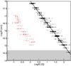 |
Fig. 11 Source extension vs. magnetic field for the UHBL models discussed by C15. The locations for the two different types of models are shown in black for the proton-synchrotron scenario and in red for the mixed lepto-hadronic scenario. The grey band indicates the range of Schwarzschild radii for the five UHBLs considered. |
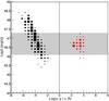 |
Fig. 12 Jet power vs. equipartition ratio for the UHBL models discussed by C15. The locations for the two different types of models are shown in black for the proton-synchrotron scenario and in red for the mixed lepto-hadronic scenario. The grey band indicates the range of Eddington luminosities for the UHBLs considered. |
Proton-synchrotron radiation dominates the high-energy spectral bump for a large set of solutions on both sides of the dividing line between different cooling regimes, as shown in Fig. 11. Because UHBLs are defined by higher peak frequencies of the high-energy bump compared to HBLs, solutions are shifted to the right, parallel to the diagonal band that marks the HBL solutions in Fig. 7. For these models, contributions from muon-synchrotron and cascade emission are negligible. The energy budget is largely dominated by the energy density of the magnetic field (cf. Fig. 12) and the jet power decreases approximately as 1 /B.
It should be noted that whether adiabatic or radiative cooling dominates at the highest proton energies depends on the assumptions made about the acceleration timescale. This explains why Mücke et al. (2003), for example, find solutions for HBLs in which both timescales are comparable at the highest energies by assuming highly efficient particle acceleration. Independently of the actual behaviour of the acceleration timescale, if one assumes that the same particle acceleration mechanism is at play in HBLs and UHBLs, it can be seen that UHBLs correspond to a more radiatively-efficient regime in which radiative losses are more important than for HBLs.
The very steep spectral shape required to fit the Fermi-LAT data in UHBLs implies that jet powers are still acceptable even with larger values of B and R compared to HBLs. It also leads to smaller values of η. For this reason, proton-photon interactions in UHBLs are largely dominated by proton-synchrotron emission and there are no “cascade bumps” even for small source extensions. The muon-synchrotron scenario does not allow us to represent the SEDs of UHBLs because the proton-synchrotron peak of the model is strongly constrained by the high-energy bump and cannot be shifted to lower energies without violating the constraints from the Fermi-LAT data.
For UHBLs, a set of mixed lepto-hadronic solutions can be found in a more compact region in log B-log R space for values of B between approximately 0.1 G and approximately 2 G, in which a combination of both SSC and proton-induced cascade emission is responsible for the high-energy spectral bump. For these models, proton-synchrotron emission occurs at intermediate energies and is very weak compared to the emission from SSC and cascades. The energy budget is dominated by the kinetic energy of the relativistic protons (cf. Fig. 12). Such mixed lepto-hadronic solutions cannot be found for less extreme HBLs when we impose our usual constraints, as was discussed in Sect. 4.4. In both scenarios applicable to UHBLs, the proton synchrotron and mixed lepto-hadronic, contribution from muon-synchrotron emission is small and there is no spectral feature in the TeV range arising from cascades.
6. Expected “cascade bump” signatures for the Cherenkov Telescope Array
The hadronic signatures in the VHE spectrum we are interested in can be seen at some level over the whole range of solutions discussed in Sect. 4. For these models, we want to test the possibility of detecting the “cascade bump” with the future CTA and thus to distinguish the hadronic scenarios from a basic one-zone SSC model.
6.1. Method
The expected spectra for CTA were simulated using the publicly available instrument response functions4 for the full southern array in the case of PKS 2155-304 and for the full northern array in the case of Mrk 421. The current layout for the southern array led to roughly a two times better differential sensitivity in the range around a few TeV compared to the northern array.
For each modelled spectrum, the integrated flux of expected γ-rays and cosmic-ray background events per energy bin was determined and weighted with the effective area from the performance file. The resulting event rate was then multiplied by the observation time, yielding the total number of detected events per bin. The number of excess events was determined by assuming that the γ-rays and cosmic rays follow a Poisson distribution and are subject to the simulated energy resolution of the instrument. The background rate was assumed to be extracted from a region on the sky that is five times larger than the “on-source” region, corresponding to a standard situation for observations in “wobble-mode”. The uncertainty in the number of excess events was calculated using the method by Li & Ma (1983). The excess and its uncertainty were then converted into a spectral point with a statistical uncertainty. An example for two simulated CTA spectra is shown in Fig. 13. For the chosen model, one can clearly see the difference in the shape of the simulated CTA spectra for an SSC and a hadronic scenario.
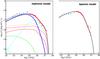 |
Fig. 13 Example of testing emission scenarios with CTA: comparison of the expected CTA spectra for two specific emission models for PKS 2155-304. A hadronic scenario is shown on the left, in which n1 = 2.1, log B [G] = 1.1. and log R [cm] = 15.6, and a standard leptonic SSC model on the right. The exposure time assumed for the simulations, 33 h, is the same as the live time for the H.E.S.S. observations, which are represented by grey data points above 3 × 1025 Hz. H.E.S.S. upper limits are not shown. Uncertainties in the CTA data points are smaller than the red squares. |
To take into account statistical fluctuations of the γ-ray rate and background rate, and the effect of a limited energy resolution, several realisations of the simulated spectra were generated. For each hadronic model we simulated one hundred spectra and compared them to one hundred spectra simulated for the SSC model for the same source. We verified that a larger number of realisations is not necessary because it does not significantly change our results.
To compare the simulated hadronic and SSC spectra, first the simulated SSC spectra were fitted with a simple logparabolic function, where the lower limit of the fitted energy range was adjusted to optimise the reduced χ2 of the fit. The form of this function, characterised with three parameters (P1, P2, P3), is given by:  (7)energies are in units of TeV and the reference energy is fixed with log E0 = −1.
The real shape of the overall SSC spectrum bump, which is absorbed on the EBL, is generally not well represented by a logparabola. However, if the energy range is restricted to energies above about 100 GeV the logparabolic function provides a satisfactory characterisation with typical fit probabilities above 10%. The same fit function is then applied to a second SSC model for each source to verify that it does indeed provide a general description of the SSC scenario and not only of a single model.
The same fit function applied to hadronic models over the same energy range usually results in worse reduced-χ2 values. An example for a logparabolic fit to a realisation of a hadronic model and of an SSC model is shown in Fig. 14.
 |
Fig. 14 Example of a logparabolic fit to realisations of simulated spectra, upper panel, for an SSC model (black circles, upper fit parameters) and a hadronic model (red squares, lower fit parameters). The spectra correspond to a 50 h exposure time on the source PKS 2155-304. The lower panel shows the ratio of the simulated fluxes over the fit function. |
It should be noted that a direct comparison between the simulated SSC and hadronic spectra, using for example a Kolmogorov-Smirnov test, risks being inconclusive. This is because we are only interested in comparing features in the spectral shape and not the absolute values of the spectral distributions between two models, which could be significantly different even between two SSC models that are acceptable solutions for the given dataset.
All spectra simulated for the SSC and hadronic models for a given source were fitted with the same function and the values of the resulting reduced χ2 were recorded. The quality of the logparabolic fit was thus used to discriminate between spectra with SSC and with hadronic shapes. The distributions of the reduced χ2 were characterised by their mean and standard deviation. As a simple ad hoc criterion, which can be refined in future studies, we consider that two models start being distinguishable if there is no overlap in their reduced χ2 distributions within one standard deviation from the mean values, meaning that if  (8)the results in the following section do not change significantly when the mean and width of a Gaussian fit to the reduced χ2 distribution is used to characterise the different models, instead of the mean and standard deviation of the distribution itself.
6.2. Detectability as a function of exposure time
The detectability of the “cascade bump” in the different hadronic models for PKS 2155-304 and Mrk 421 was tested for three different observation times with CTA: 20 h, 50 h, and 100 h. These are typical exposure times used with current IACT arrays on a single source when considering that the low-state flux can be summed over several observation periods. Both blazars chosen for this study will be observed regularly with CTA, as calibration sources, but also within the AGN Key Science Programme (CTA Consortium, in prep.).
The logparabolic function provides a good fit for two independent SSC models for each of the two sources. In the case of PKS 2155-304, we compare an SSC model that includes the optical points against an alternative model that is not constrained by the optical emission, supposed in this case to stem from a different emission region, for example an extended jet. The reduced χ2 distributions for one hundred realisations of each of the two SSC models are in good agreement for 20 h and 50 h exposure times and still have a large overlap for 100 h. The 1-σ envelope of the resulting reduced χ2 distributions for fits above approximately 400 GeV is below 1.3 for observations of 20 h or 50 h and below 2.4 for observations of 100 h at which point the shapes of the simulated SSC spectra do not always match the logparabolic function very well.
In the case of Mrk 421, we compare two SSC models with Doppler factors of δ = 30 and 50, with logparabolic fits above approximately 600 GeV. The 1-σ envelope is below 1.5 for 20 h and 50 h exposure times and increases to 2.0 for 100 h.
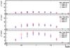 |
Fig. 15 Mean values of the reduced χ2 distributions of logparabolic fits to one hundred realisations of each model for the SEDs of PKS 2155-304. The abscissa shows the logarithm of the magnetic field strength to distinguish different hadronic models. The error bars show the standard deviation of the distributions. The energy range of the fit was chosen to provide a good reduced χ2 for two different SSC models. The grey band is the union of the 1-σ envelopes of those SSC spectrum fits. |
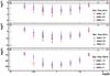 |
Fig. 16 Mean logarithmic values of the probabilities for the same fits as Fig. 15 for PKS 2155-304. The abscissa shows the logarithm of the magnetic field strength to distinguish different hadronic models. The error bars show the standard deviation of the distributions. The grey band is the union of the 1-σ envelopes of the SSC spectrum fits. |
 |
Fig. 17 Mean values of the reduced χ2 distributions of logparabolic fits to one hundred realisations of each model for the SEDs of Mrk 421. The caption of Fig. 15 contains more details. |
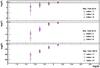 |
Fig. 18 Mean logarithmic values of the probabilities for the same fits as Fig. 17 for Mrk 421. The abscissa shows the logarithm of the magnetic field strength to distinguish different hadronic models. The error bars show the standard deviation of the distributions. The grey band is the union of the 1-σ envelopes of the SSC spectrum fits. |
When the same logparabolic fits are applied to the hadronic models, in most cases the reduced χ2 of the fit is different from that obtained with the SSC model by more than one standard deviation for 50 h of observation time, and in several cases already by 20 h (cf. Figs. 15 and 17). The difference between SSC and hadronic models becomes clearer as the exposure time increases. When investing 100 h of observation time, the large majority of our hadronic models for PKS 2155-304 and for Mrk 421 are clearly distinguishable from the SSC models. Figures 16 and 18 show the corresponding fit probabilities (p-values) in terms of the mean and standard deviation for the distributions of the logarithmic probabilities. For 50 h of observation time, for example, most hadronic models for PKS 2155-304 have probabilities less than 1 × 10⁻⁵, whereas the SSC models have probabilities greater than 0.1.
For PKS 2155-304, the model with a spectral index of 2.1 and a very small magnetic field of 1 G corresponds to a pure proton-synchrotron scenario, in which contributions from muon-synchrotron and cascades are very small and do not lead to significant features. This model is also the one with the largest jet power. On the other hand, models with very large magnetic fields of B ≳ 70 G and dense emission regions also present a challenge, because the contribution from cascades and muon synchrotron are strongly absorbed at the highest energies, leading to very steep and smooth spectra without detectable features. These models are also disfavoured on physical grounds, because the radius of the emission region is very close to the Schwarzschild radius of the source.
Pure proton-synchrotron models for Mrk 421 do not exist, as discussed above. Models with very large magnetic fields above ≳ 100 G suffer from the same problems for detection of the “cascade bump” as in the case of PKS 2155-304. They are again disfavoured due to the smallness of the emission region.
6.3. Detectability as a function of flux level and redshift
The two sources selected for this case study are particularly bright HBLs, even in their low states. To test how the detectability of the “cascade bump” depends on the absolute flux level, we scaled the fluxes of an SSC model and of a well distinguishable hadronic model by factors between 0.5 and 0.1 for each of the sources.
For a model for PKS 2155-304 with a “cascade bump” detectable in 20 h exposure time, at least 50 h are needed for a detection of the signature when the flux is reduced to 40% of its initial value. For a reduction to 30%, more than 100 h are needed. When selecting a well-distinguishable model for Mrk 421, in which the “cascade bump” is detected in 20 h, and reducing its flux to 40% of its initial value, again the signature is only detectable in 50 h of exposure time or more. Around 100 h are needed for a flux reduced to 30%. Thus only sources with relatively high flux levels during their low states may be considered for searches of this spectral signature with CTA.
The HBLs PKS 2155-304 and Mrk 421 are nearby sources with redshifts of z = 0.116 and z = 0.031, respectively. To test the dependence of the “cascade bump” signature on the source distance, we artificially redshifted an SSC model and a hadronic model with well-detectable “cascade bumps” to values of z = 0.15, 0.2 for PKS 2155-304 and to z = 0.1, 0.15, 0.2 for Mrk 421, and evaluated the fit results for these shifted fluxes. Unsurprisingly, the source redshift is a very important factor for the detectability of the hadronic signature. For PKS 2155-304, moving the redshift to 0.15 increases the minimum exposure time for a detection of the signature from 20 h to 50 h. In the case of Mrk 421, putting the source at a redshift of 0.1 already increases the required observation time from 20 h to 100 h. Increasing the source distance leads not only to a reduction of the observed flux, but the stronger absorption on the EBL rapidly washes out the spectral structure at the highest energies.
It should be stressed that the detectability of the hadronic signature does not only depend on the flux level and redshift of the source, but also on its intrinsic spectral shape. The above estimates based on our two sources are meant to provide some general trends, although actual numbers might vary significantly for other sources. Sources with large high-energy bumps and hard spectra in the TeV range might prove especially more accessible, even at larger redshifts and for lower fluxes.
7. Discussion
7.1. Impact of our simplifying assumptions
To arrive at the selection of models for the two HBL sources, several physically-motivated simplifying assumptions were made to reduce the space of the model parameters. They are discussed in the following paragraphs.
Assuming an identical index for the injection spectra of protons and primary electrons significantly reduces the acceptable values of the slope for both spectra and excludes pure proton-synchrotron scenarios for the SED of Mrk 421, given the constraints from the optical data. It also restricts the minimum jet power for the solutions for PKS 2155-304, by excluding solutions with n1< 1.9. This assumption ignores the complexity of the actual acceleration mechanisms that may be at play inside the source and might lead to different particle spectra for protons and leptons, which are subject to diffusion on different length scales. In the same sense, the assumption of a pure synchrotron cooling break in the electron spectrum might be an over-simplification, as is generally assumed in one-zone SSC models. Nevertheless, the parameter space of our solutions should not change significantly for particle indices before cooling that are close to the value of around two, which is expected for Fermi-like acceleration. The stronger constraint comes from the fact that primary electrons are completely cooled whereas protons are not, resulting in a significantly steeper stationary spectrum for the electrons. This constraint is a solid consequence of the assumed co-acceleration scenario.
The maximum proton energy is determined by an equilibrium between acceleration and loss timescales, and thus in our framework only by the magnetic field B and source radius R. A more sophisticated treatment of particle acceleration, diffusion, and energy loss may lead to a wider range of maximum possible proton energies for a given parametrisation of the source conditions. More diverse combinations between the proton-synchrotron component and the muon-synchrotron and cascade components might occur. As an order-of-magnitude estimate, however, the current approach is sufficient.
We chose to fix the value of the bulk Doppler factor to δ = 30, but the present study may be extended to a range of values. We verified the effect on the resulting models for a given B when varying the Doppler factor to δ = 20 and to δ = 40 while keeping the peak positions and peak fluxes of the modelled SEDs constant. Increasing δ by a factor fδ leads to an increase in the observed energy flux level “νFν” that is proportional to  . At the same time, the frequencies of the electron-synchrotron and proton-synchrotron peak positions increase by a factor fδ. A reduction in R, which leads to a reduction in γp;max given our constraints, and an adjustment of the maximum electrons Lorentz factor γe;max, are necessary to keep the positions of the peaks fixed at their initial frequencies.
Reducing R leads to a linear reduction of γp;max and thus to a quadratic reduction in the proton-synchrotron peak frequency. When compensating for the shift in the peak frequency by reducing R by a factor  , the flux level decreases by a factor
  . It is thus still a factor
  higher than before the change in δ. This remaining flux increase needs to be offset by reducing the particle densities by a factor
  . For the proton population, this reduced particle density leads to a smaller contribution from the muon-synchrotron and cascade components. Inversely, these components become more significant when lowering the value of δ while keeping the flux level and peak frequencies seen by the observer fixed. The low-energy turnover of the modelled SED in the optical range is kept fixed by decreasing the value of γmin,e when increasing δ, which can lead to more standard values for certain models.
The choice of δ has also an effect on the jet power. Given the small-angle approximation (Eq. (2)), the jet power is directly proportional to δ2, as can be seen from Eq. (4). When neglecting the small contributions from the electron population and from the radiation fields, the jet power takes the following form in our approximation:  (9)with c1 and c2 constant. For a given B, when keeping flux level and peak positions fixed as discussed above, the jet power Lj increases linearly with δ if the jet is dominated by the magnetic energy density uB, due to the impact of the factors R2 and δ2. For a jet dominated by the kinetic energy density of the proton population up and for a proton spectrum with index n1 ~ 2, the jet power changes as
  as a consequence of the additional changes in Kp and γp,max.
For a typical model for PKS 2155-304, initially in the up dominated regime, increasing δ from 20 to 40 while adjusting flux level and synchrotron peak positions leads to a decrease in Lj by about 15% and a drop in the flux level of the muon-synchrotron and the cascade components of roughly a factor of two in νFν. For values of δ in the usual range assumed for blazar emission models, the results presented here should thus not change fundamentally.
To constrain the total jet power for our solutions, we compare it to the Eddington luminosity as a natural scale defined by the mass of the central black hole. This is clearly meant as an order-of-magnitude estimate for the maximum acceptable jet power instead of a strict limit. A different approach would be to consider the disk luminosity as a natural scale to compare to the jet power. However, the disk luminosity depends on the radiative efficiency and thus on the physical conditions of the accretion disk, which is in general not observationally accessible, especially for BL Lac objects, and for which a multitude of models exist. In blazars it is generally seen that the jet power is not limited by the disk luminosity, even for the “standard” leptonic models (e.g. Celotti & Ghisellini 2008; Ghisellini et al. 2010). In the case of Mrk 421, one can estimate the disk luminosity from the detectable emission of the broad line region. Sbarrato et al. (2012) provide a value of 0.5 × 1042 erg s-1 for the luminosity of the broad line region for this source, translating to roughly 1043 erg s-1 for the disk luminosity (see e.g. Ghisellini 2013), meaning about 5 × 10⁻⁴Ledd,Mrk421. For a typical jet power of 0.03 Ledd,Mrk421 (cf. Fig. 8), the ratio of jet power over disk luminosity would be less than 100. Although these values still require a relatively inefficient accretion process, the hadronic interpretation for HBLs does not suffer from the extreme energetic requirements derived by Zdziarski & Böttcher (2015) for a set of hadronic models, which they applied to FSRQs and low- and intermediate-frequency-peaked BL Lac objects.
The study presented here was carried out using the model of the EBL by Franceschini et al. (2008), which is frequently used for the interpretation of VHE data and has been shown to be consistent with a range of observed sources (Biteau & Williams 2015). Although the dependency of our results on the chosen model is not very strong, given that the sources under study are not very distant, we note that it was shown that the “cascade bump” signature becomes less well defined when assuming a higher opacity of the EBL (Zech et al. 2013). On the other hand, models with a more transparent EBL favour a detection of the signature.
Any change in the CTA performance curves also has an impact on our results. When studying for example the detectability of the Mrk 421 models with the southern performance files, one clearly sees a significant improvement due to the better coverage at the highest energies that comes from a larger number of medium-sized telescopes and the additional small-size telescopes not foreseen for the northern site. Models with undetectable “cascade bumps” for 100 h exposures with the northern performance curves show clear detectability when using the southern performance curves instead. The public performance curves used here represent preliminary expectations of the instrumental response functions for preliminary array layouts. Once the actual performance of the final CTA arrays is established the results might thus differ from our current predictions.
The long exposure times of up to 100 h for the study that we are proposing require multiple separate pointings during the visibility periods of the sources. These pointings will be taken over several months or even years and will very likely contain data from different flux states. When extracting a spectrum from these data, one will have to be very careful with the treatment of flux and spectral variability. As discussed by Abdo et al. (2011) in the case of a long-term campaign on Mrk 501, it will be important to exclude periods of flaring activity to build the spectrum from data in a low, persistent flux level. Based on past observations of HBLs with the current generation of Cherenkov telescopes, it seems that significant spectral variability in the VHE band occurs only during flaring episodes. Although some flux variability was detected in the long-term low-state VHE lightcurve of Mrk 421 (Aleksić et al. 2015), significant spectral variability was seen neither in the Fermi-LAT data from 0.1 to 400 GeV, nor in the MAGIC data over the 4.5 months of observations (Abdo et al. 2011). Long-term VHE data from PKS 2155-304 from H.E.S.S. also indicate only very small spectral variations during non-flaring periods (Abramowski et al. 2010), which has been confirmed with more recent data (Chevalier et al. 2016). The risk of introducing spectral features due to a combination of data from different periods should thus be small if the datasets are carefully selected and combined.
A final but important point concerns the method applied in this study to characterise spectral features in the simulated SEDs. The fit, by χ2 minimisation, of a simple function to the simulated spectrum points represents a robust and rapid first approach, but more sophisticated techniques will certainly be applied to analyse CTA spectra. For the spectral analysis of current IACT data, maximum likelihood methods applied to forward folding of different spectral shapes have become a standard technique. The direct analysis of VHE data using realistic model shapes as underlying hypothesis, instead of power laws and logparabola, possibly through the use of libraries of modelled SEDs over a range of acceptable parameters, would be a next step and could be built on current techniques used for the analysis of X-ray data. Ideally, one would apply such methods to a full and simultaneous MWL dataset. It can thus be realistically expected that the search for spectral features in actual CTA data will be more effective than the simple approach proposed here for a first evaluation of the detectability of the “cascade bump”.
7.2. Additional constraints from variability
Even in the relatively low states the present study is focusing on, some flux variability was found during the MWL campaigns of Mrk 421 and PKS 2155-304. For the latter source, Aharonian et al. (2009a) report a small overall variability, characterised by fractional rms, at the 30% level in the MWL light curves of the campaign that covered twelve nights. The optical, X-ray, and VHE light curves show flux-doubling on timescales of days. For Mrk 421, Abdo et al. (2011) report only low flux variability during the 2009 campaign that covered 4.5 months. A more in-depth study by Aleksić et al. (2015) finds significant variability at all wavelengths, which is highest in X-rays, with variations that are typically smaller than a factor of two. The authors find variability in the X-ray and VHE bands on day timescales, and in the optical and UV band on weekly or longer timescales.
When requiring that the size of the emission region be sufficiently small for the assumed Doppler factor δ = 30, to allow for variability of the order of one day one can use the usual light-crossing time argument to arrive at a limiting radius:  (10)This translates into a constraint on the source extension of R ≲ 7 × 1016 cm for both sources. Although this kind of an additional constraint would be of no consequence for our selection of models for Mrk 421, which already present small emission regions, a few models for PKS 2155-304 would be excluded. This concerns the models with the most important jet powers.
Apart from variability timescales, correlated behaviour between different wavelength bands is another observable characteristic that might help distinguish leptonic from hadronic scenarios. Aharonian et al. (2009a) find a correlation between the optical and VHE bands for PKS 2155-304 on timescales of days, but no correlation between optical and Fermi-LAT data. Although our stationary model does not permit us to study variability, the scenarios that ascribe the Fermi-LAT flux to proton-synchrotron emission and the VHE flux mostly to muon-synchrotron emission might explain a difference in the variability patterns between these two domains, if confirmed. Muon-synchrotron emission is a consequence of proton-photon interactions and thus subject to correlated variations with the target photon field, meaning the electron-synchrotron emission responsible for the optical and X-ray spectrum in our interpretation, although time-lags between the high- and low-energy components would need to be evaluated for a given set of source parameters.
According to Aleksić et al. (2015), Mrk 421 shows a positive correlation between the VHE and X-ray fluxes with zero time lag during the 2009 MWL campaign. The authors claim that as a consequence, the direct high-energy correlation supports leptonic models over hadronic ones. In general, correlated behaviour between the different energy bands in the lepto-hadronic model can be accounted for in a co-acceleration or co-injection scenario and via the proton-photon interactions. However, the detailed behaviour can be complex and needs to be studied with time-dependent models (e.g. Mastichiadis et al. 2013; Diltz et al. 2015).
The authors also report an anticorrelation between the optical and UV band on the one hand, and the X-ray band on the other, whereas they report that there does not seem to be a correlation with the radio band. If the emission in the optical and UV band and the X-ray emission come from different emission regions and the anticorrelation is a coincidence, we would have less constraints on our model on the n1 parameter, but might require higher γe;min values because the optical and UV data would still present upper limits.
7.3. Non-uniqueness of the “cascade bump” signature
An obvious limitation of the present study is the fact that the hadronic models were only compared to the most standard one-zone SSC models. More complex scenarios might well produce comparable spectral hardening in the VHE spectra, but the higher degree of complexity that is generally accompanied by a larger number of free parameters would need to be well justified against the basic hadronic scenario proposed here. A potentially similar spectral feature might arise in the scenarios discussed in the following paragraphs.
Emission from second-order SSC, meaning a second upscattering of a fraction of high-energy photons on the relativistic electrons in a standard SSC model, could in principle lead to an additional spectral component at high energies. In the case of HBLs however, this component is in general completely negligible compared to first-order SSC. Inverse-Compton upscattering of the bulk of the first-order SSC photons on the electron population around the break energy would take place deeply within the Klein-Nishina regime.
A different effect that can lead to spectral hardening in the radiative emission from electrons is described by Moderski et al. (2005). In sources with strong external photon fields, where electron cooling is dominated by the Inverse Compton process, a hardening or pile-up in the steady-state electron spectrum can form for energies where cooling becomes ineffecient due to Klein-Nishina effects. This would result in an upturn or “bump” in the synchrotron spectrum. However, the effect is expected to be negligible for the high-energy Inverse Compton spectrum, where the hardening of the steady-state electrons is in competition with a softening of the emission due to the same Klein-Nishina effects. We would thus not expect an appreciable feature from this effect, particularly for HBLs, for which external photon fields can usually be neglected and synchrotron cooling dominates over Inverse Compton cooling for the electron population.
Multi-zone SSC models could in principle generate spectral hardening at TeV energies. One could image emission from a first zone dominating the SED over almost the entire observable energy range, whereas SSC emission from a second, more compact zone would only only appear at VHE energies. Although the Klein-Nishina effect would limit the high-energy reach of a second SSC component, this kind of a scenario could still be possible and might be difficult to distinguish from the hadronic “cascade bump”. Information on spectrally resolved variability might be needed to rule against or in favour of each scenario.
An additional spectral component in leptonic models might also arise from external Compton emission caused by the upscattering of photons from external fields, such as broad line region, disk emission, dust torus, stellar radiation field, etc. For HBLs, this kind of a component is not expected to contribute significantly to the SED due to the weakness or absence of the non-detectable external photon fields. If such a component was present, potential VHE features would also be limited by the Klein-Nishina effect.
Spectral hardening in the VHE band might arise for scenarios in which γ-rays in a certain energy range are absorbed on external photon fields in the source, for example from the broad line region (Senturk et al. 2013; Poutanen & Stern 2010), accretion disk, or torus (Donea & Protheroe 2003), and where the flux recovers at higher energies. However, these kinds of absorption features would be expected to occur instead in the Fermi-LAT band with a flux recovery in the low VHE band. Besides, as discussed above, although external photon fields are very likely to play an important role for flat-spectrum radio quasars, they are usually considered negligible for HBLs (see also the discussion by Abramowski et al. 2013).
Spectral hardening in the VHE range is also predicted by scenarios in which ultra-energetic photons or protons escape from the source and trigger particle cascades by interactions with the EBL and cosmic microwave background (CMB; e.g. Aharonian et al. 2002; Essey et al. 2011; Murase et al. 2012; Aharonian et al. 2013; Taylor et al. 2011). However, this kind of a component would be expected for sources with relatively high redshifts. It would also not exhibit the same spectral shape and temporal behaviour.
7.4. Prospects for current and future Imaging Air Cherenkov telescope arrays
The HBL PKS 2155-304 is frequently observed with the H.E.S.S. IACT array. According to Chevalier et al. (2016), about 260 h of data were taken between 2004 and 2012, excluding the very luminous flares seen in 2006. Even so, the long-term light curve shows flux variations by a factor of a few. When assuming, very roughly, a ten times better sensitivity for CTA with respect to H.E.S.S., the currently available VHE dataset on this source would correspond to maybe 40 h of an equivalent CTA exposure. This would include different flux states and does not account for the increasing gap between the current IACT sensitivities and the expected CTA performance at energies above a few TeV, where the additional performance of the small-size telescopes in the southern array becomes important (Bernlöhr et al. 2013). It would in any case be interesting to study the complete set of available data to probe the most prominent “cascade bump” features. A similarly rich dataset might also be available on Mrk 421 from observations with the MAGIC and VERITAS IACTs. For this blazar, 840 h of TeV data had been collected with the Whipple IACT (Acciari et al. 2014), albeit with a lower sensitivity than current arrays.
The two sources we have studied here are foreseen to be observed frequently with CTA. Given their brightness in the VHE range, they will be used as calibration sources and they are also prominently included in the proposed AGN Key Science Project (CTA Consortium, in prep.). Their long-term light curve will be studied with regular observations over an important fraction of the lifetime of CTA. Deep exposures over shorter time ranges are also foreseen, to help derive high-quality spectra in a single state. Even if observation times of up to 100 h will be difficult to achieve over a short time range, observations from a few seasons could be summed, as long as the sources show sufficiently similar flux states.
In general, nearby bright HBLs are expected to be the best candidates to search for the “cascade bump” signature. According to the TeVCAT catalogue (see footnote on page 2) there are currently twenty-two known VHE emitting HBLs with z< 0.15 that could be considered for such a search, but only the sources with high fluxes during low states are promising targets. Apart from PKS 2155-304 and Mrk 421, about twelve known HBLs seem promising targets when excluding UHBLs and sources with very faint fluxes, meaning below 2% of the Crab flux above 200 GeV, in low or average states: Mrk 501, PKS 2005-489, RGB J0152+017, 1ES 1959+650, 1ES 2344+514, 1ES 1727+ 502, IC 310, 1ES 0806+524, 1ES 1215+303, B3 2247+381, 1ES 1741+196, and PKS 1440-389 although it has an uncertain redshift.
Additional target candidates could be searched amongst the eight VHE HBLs currently known without redshifts and amongst a handful of nearby intermedium-frequency peaked BL Lac objects (IBL). However, in the latter, external photon fields might no longer be negligible, which would further complicate the search for hadronic signatures.
In the case of a non-detection of the suggested spectral hardening with CTA after an accumulated observation time of about 100 h, hadronic interpretations of the SEDs of the sources in question would become strongly constrained. The most feasible models, when considering the required source extension and energetics, would be rejected. This would at least permit us to strongly reduce the available parameter space for one-zone hadronic solutions. Combined with future observational constraints on the variability timescale during the low state, one-zone hadronic solutions might be ruled out entirely. How such an assessment would be modified when loosening the constraints on co-acceleration and γp,max will need to be investigated further.
7.5. Ultra-high-energy cosmic rays and high-energy neutrinos
The maximum energy of the proton population is constrained by a comparison of the assumed acceleration timescale and the shortest cooling timescale, as explained in Sect. 2. For Mrk 421, we find maximum proton Lorentz factors up to γp,max ~ 1 × 10⁹ for the models presented here that correspond to an energy of about 1018 eV. Proton-synchrotron solutions for PKS 2155-304 with large extensions of the emission region around 1017 cm have γp,max values up to about 1010, meaning proton energies up to about 1019 eV. When accounting for Doppler boosting of the particle energies, certain solutions permit us thus to reach maximum proton energies close to what is required to account for the most energetic UHECRs, based on our simplistic description of the acceleration and loss timescales. In addition, a rapidly decreasing fraction of protons with Lorentz factors above γp,max is expected from the exponential tail of the particle distribution. The most energetic UHECRs might however be nuclei (e.g. Abbasi et al. 2016), which we do not consider in our code, instead of protons.
The use of the Monte Carlo code SOPHIA allows us to directly extract the neutrino spectra for a given model, which only needs to be transformed to the observer frame on Earth. As detailed in Cerruti et al. (2015), we carefully account for the radiative cooling of muons before extracting the neutrino spectra resulting from muon decay. The expected neutrino flux is directly related to the importance of proton-photon interactions inside the source, when ignoring potential neutrino production through neutron decay and UHECR interactions outside of the source. Scanning the parameter space for a given source instead of proposing only a single solution makes it possible to estimate a range of possible neutrino spectra for the source within our lepto-hadronic framework.
Figures 19 and 20 show two solutions each for the two HBLs under study, for models with different magnetic field strengths. Although the relatively small parameter space of hadronic solutions for Mrk 421 is reflected in a small difference between the expected neutrino spectra for this source, the spread is much more significant in the case of PKS 2155-304. For the latter, solutions close to the pure proton-synchrotron scenario lead to a low flux with a high energy peak, whereas solutions with a significant contribution from muon-synchrotron and cascade emission result in higher neutrino fluxes with lower peak energies.
 |
Fig. 19 Expected neutrino spectra on Earth (all flavours combined) for two hadronic models for PKS 2155-304. “Model 1” has a small log B [G] = 0.3, whereas “Model 2” has a much larger log B [G] = 1.9. |
 |
Fig. 20 Expected neutrino spectra on Earth (all flavours combined) for two hadronic models for Mrk 421. “Model 1” has a log B [G] = 1.5, whereas “Model 2” has a log B [G] = 2.1. |
Contrary to the lepto-hadronic models discussed by Petropoulou et al. (2015), which have a small γp,max, large jet power, and are dominated by proton-photon interactions, the models selected following our criteria lead to neutrino spectra that peak at higher energies. For the sources studied here, the expected neutrino emission seems out of reach for the IceCube telescope (cf. Aartsen et al. 2014) when considering low γ-ray flux states. Flaring activity, if related to hadronic processes, can significantly increase the neutrino production, as discussed by Petropoulou et al. (2016). Next-generation instruments with a higher energy reach, like ARA (Allison et al. 2016) or GRAND (Martineau-Huynh et al. 2016), might have a better chance of reaching the required high-energy sensitivity for a detection in this scenario. A more in-depth study of this topic will be treated in a dedicated publication.
8. Conclusions
We explore the parameter space of the one-zone hadronic blazar emission model for two bright VHE HBLs, PKS 2155-304 and Mrk 421, during low emission states. Satisfactory realisations of the model, where the high-energy emission is interpreted as a combination of proton-synchrotron, muon-synchrotron and proton-photon induced cascade emission, can be found for a range of parameters. The muon-synchrotron and cascade emission become more prominent as the density of the emission region is increased while its size is reduced. The TeV spectrum can be dominated by proton-synchrotron or muon-synchrotron emission, depending on the chosen solution.
The mixed lepto-hadronic models found for UHBLs (C15) for magnetic fields of strengths intermediate between those for typical proton-synchrotron and SSC models do no provide satisfactory solutions for the HBLs under study, given our choice of simplifying assumptions about the particle populations and on the acceptable jet power. Muon-synchrotron emission, on the other hand, cannot dominate the TeV spectrum for UHBLs. Thus HBLs and UHBLs seem to populate distinct parameter spaces of the lepto-hadronic one-zone model.
All the hadronic models found for the two sources under study show a hardening in the multi-TeV spectrum at some level, due to the emission from synchrotron-pair cascades that are induced by proton-photon interactions. This adds to the dominant proton- or muon-synchrotron emission at these energies. Using a simple logparabolic fit to distinguish between the expected spectral shapes from pure SSC and from hadronic emission, we show that this characteristic “cascade bump” should be detectable for most models with CTA within 50 h, or in a few cases within 100 h, of observation time. This is especially the case for those models that present preferred solutions due to low jet powers and plausible extensions of the emission region. The faint spectral feature is only expected to be detectable in nearby HBLs, of redshifts smaller than approximately 0.15 and with flux levels at least a few tenths of those of the sources under study. We identify of the order of ten known TeV blazars that might be considered for future searches for such a signature. Although the “cascade bump” permits the distinction between a standard one-zone SSC model and a simple one-zone hadronic model, confusion with signatures from more complex SSC scenarios has not been studied here and cannot be excluded a priori.
For an up-to-date catalogue of TeV sources, see http://tevcat.uchicago.edu
An alternative definition of “hadronic” models, where the whole SED is dominated by emission linked to hadrons, is used by Mastichiadis et al. (2013). Such scenarios seem to lead to very high jet powers and are not considered here.
Compared to C15, the jet powers shown here are larger by a factor of two to account for double-sided jets.
Acknowledgments
The authors wish to acknowledge discussions with C. Boisson, H. Sol, S. Inoue, D. Pelat, G. Henri, A. Reimer, J.-P. Ernenwein, and L. Stawarz that greatly helped improve this work. This paper has gone through internal review by the CTA Consortium.
References
- Aartsen, M. G., Abbasi, R., Abdou, Y., et al. 2013, Science, 342, 1242856 [Google Scholar]
- Aartsen, M. G., Ackermann, M., Adams, J., et al. 2014, ApJ, 796, 109 [Google Scholar]
- Abbasi, R., Bellido, J., Belz, J., et al. 2016, Proc. International Symposium for Ultra-High Energy Cosmic Rays (UHECR2014), id. 010016 [Google Scholar]
- Abdo, A. A., Ackermann, M., Ajello, M., et al. 2011, ApJ, 736, 131 [Google Scholar]
- Abramowski, A., Acero, F., et al. (H.E.S.S. Collaboration) 2010, A&A, 520, A83 [NASA ADS] [CrossRef] [EDP Sciences] [Google Scholar]
- Abramowski, A., Acero, F., et al. (H.E.S.S. Collaboration) 2012, A&A, 539, A149 [NASA ADS] [CrossRef] [EDP Sciences] [Google Scholar]
- Abramowski, A., Acero, F., et al. (H.E.S.S. Collaboration) 2013, A&A, 552, A118 [NASA ADS] [CrossRef] [EDP Sciences] [Google Scholar]
- Acciari, V. A., Arlen, T., Aune, T., et al. 2014, Astropart. Phys., 54, 1 [Google Scholar]
- Acharya, B. S., Actis, M., Aghajani, T., et al. 2013, Astropart. Phys., 43, 3 [Google Scholar]
- Ackermann, M., Ajello, M., Allafort, A., et al. 2011, ApJ, 743, 171 [NASA ADS] [CrossRef] [Google Scholar]
- Actis, M., Agnetta, G., Aharonian, F., et al. 2011, Exp. Astron., 32, 193 [NASA ADS] [CrossRef] [Google Scholar]
- Aharonian, F. A., Timokhin, A. N., & Plyasheshnikov, A. V. 2002, A&A, 384, 834 [NASA ADS] [CrossRef] [EDP Sciences] [Google Scholar]
- Aharonian, F., Akhperjanian, A. G., Bazer-Bachi, A. R., et al. 2007, ApJ, 664, L72 [Google Scholar]
- Aharonian, F., Akhperjanian, A. G., Anton, G., et al. 2009a, A&A, 508, 561 [NASA ADS] [CrossRef] [EDP Sciences] [Google Scholar]
- Aharonian, F., Akhperjanian, A. G., Anton, G., et al. 2009b, ApJ, 696, L150 [NASA ADS] [CrossRef] [Google Scholar]
- Aharonian, F., Essey, W., Kusenko, A., & Prosekin, A. 2013, Phys. Rev. D, 87, 063002 [Google Scholar]
- Albert, J., Aliu, E., Anderhub, H., et al. 2007, ApJ, 669, 862 [Google Scholar]
- Aleksić, J., Ansoldi, S., Antonelli, L. A., et al. 2015, A&A, 576, A126 [NASA ADS] [CrossRef] [EDP Sciences] [Google Scholar]
- Allison, P., Bard, R., et al. (ARA Collaboration) 2016, Phys. Rev. D, 93, 082003 [Google Scholar]
- Bernlöhr, K., Barnacka, A., Becherini, Y., et al. 2013, Astropart. Phys., 43, 171 [Google Scholar]
- Bettoni, D., Falomo, R., Fasano, G., & Govoni, F. 2003, A&A, 399, 869 [NASA ADS] [CrossRef] [EDP Sciences] [Google Scholar]
- Biermann, P. L., & Strittmatter, P. A. 1987, ApJ, 322, 643 [Google Scholar]
- Biteau, J., & Williams, D. A. 2015, ApJ, 812, 60 [NASA ADS] [CrossRef] [Google Scholar]
- Bosch-Ramon, V., Perucho, M., & Barkov, M. V. 2012, A&A, 539, A69 [NASA ADS] [CrossRef] [EDP Sciences] [Google Scholar]
- Böttcher, M., Reimer, A., Sweeney, K., & Prakash, A. 2013, ApJ, 768, 54 [Google Scholar]
- Cavagnolo, K. W., McNamara, B. R., Nulsen, P. E. J., et al. 2010, ApJ, 720, 1066 [NASA ADS] [CrossRef] [Google Scholar]
- Celotti, A., & Ghisellini, G. 2008, MNRAS, 385, 283 [NASA ADS] [CrossRef] [Google Scholar]
- Cerruti, M., Boisson, C., & Zech, A. 2013, A&A, 558, A47 [EDP Sciences] [Google Scholar]
- Cerruti, M., Zech, A., Boisson, C., & Inoue, S. 2015, MNRAS, 448, 910 [Google Scholar]
- Chevalier, J., Kastendieck, M. A., Rieger, F., et al. 2016, ArXiv e-prints [arXiv:1509.03104] [Google Scholar]
- Dermer, C. D., & Atoyan, A. 2001, ArXiv [astro-ph/0107200] [Google Scholar]
- Dermer, C. D., Murase, K., & Takami, H. 2012, ApJ, 755, 147 [Google Scholar]
- Dermer, C. D., Cerruti, M., Lott, B., Boisson, C., & Zech, A. 2014, ApJ, 782, 82 [Google Scholar]
- Diltz, C., Böttcher, M., & Fossati, G. 2015, ApJ, 802, 133 [Google Scholar]
- Dimitrakoudis, S., Mastichiadis, A., Protheroe, R. J., & Reimer, A. 2012, A&A, 546, A120 [NASA ADS] [CrossRef] [EDP Sciences] [Google Scholar]
- Dimitrakoudis, S., Petropoulou, M., & Mastichiadis, A. 2014, Astropart. Phys., 54, 61 [Google Scholar]
- Donea, A.-C., & Protheroe, R. J. 2003, Astropart. Phys., 18, 377 [Google Scholar]
- Essey, W., & Kusenko, A. 2010, Astropart. Phys., 33, 81 [Google Scholar]
- Essey, W., Kalashev, O., Kusenko, A., & Beacom, J. F. 2011, ApJ, 731, 51 [Google Scholar]
- Fossati, G., Maraschi, L., Celotti, A., Comastri, A., & Ghisellini, G. 1998, MNRAS, 299, 433 [Google Scholar]
- Franceschini, A., Rodighiero, G., & Vaccari, M. 2008, A&A, 487, 837 [NASA ADS] [CrossRef] [EDP Sciences] [Google Scholar]
- Gaidos, J. A., Akerlof, C. W., Biller, S., et al. 1996, Nature, 383, 319 [Google Scholar]
- Ghisellini, G. 2013, in Eur. Phys. J. Web Conf., 61, 05001 [Google Scholar]
- Ghisellini, G., Tavecchio, F., Foschini, L., et al. 2010, MNRAS, 402, 497 [Google Scholar]
- Hervet, O., Boisson, C., & Sol, H. 2015, A&A, 578, A69 [NASA ADS] [CrossRef] [EDP Sciences] [Google Scholar]
- Hervet, O., Boisson, C., & Sol, H. 2016, A&A, 592, A22 [NASA ADS] [CrossRef] [EDP Sciences] [Google Scholar]
- Hillas, A. M. 1984, ARA&A, 22, 425 [Google Scholar]
- Katarzyński, K., Sol, H., & Kus, A. 2001, A&A, 367, 809 [NASA ADS] [CrossRef] [EDP Sciences] [Google Scholar]
- Katarzyński, K., Ghisellini, G., Tavecchio, F., Gracia, J., & Maraschi, L. 2006, MNRAS, 368, L52 [Google Scholar]
- Konigl, A. 1981, ApJ, 243, 700 [NASA ADS] [CrossRef] [Google Scholar]
- Kotilainen, J. K., Falomo, R., & Scarpa, R. 1998, A&A, 336, 479 [NASA ADS] [Google Scholar]
- Li, T.-P., & Ma, Y.-Q. 1983, ApJ, 272, 317 [NASA ADS] [CrossRef] [Google Scholar]
- Mannheim, K. 1993, A&A, 269, 67 [NASA ADS] [Google Scholar]
- Martineau-Huynh, O., Kotera, K., Bustamente, M., et al. 2016, in Eur. Phys. J. Web Conf., 116, 03005 [Google Scholar]
- Mastichiadis, A., Petropoulou, M., & Dimitrakoudis, S. 2013, MNRAS, 434, 2684 [Google Scholar]
- McLure, R. J., & Dunlop, J. S. 2002, MNRAS, 331, 795 [Google Scholar]
- Moderski, R., Sikora, M., Coppi, P. S., & Aharonian, F. 2005, MNRAS, 363, 954 [Google Scholar]
- Mücke, A., & Protheroe, R. J. 2001, Astropart. Phys., 15, 121 [Google Scholar]
- Mücke, A., Engel, R., Rachen, J. P., Protheroe, R. J., & Stanev, T. 2000, Comput. Phys. Commun., 124, 290 [Google Scholar]
- Mücke, A., Protheroe, R. J., Engel, R., Rachen, J. P., & Stanev, T. 2003, Astropart. Phys., 18, 593 [Google Scholar]
- Murase, K., Dermer, C. D., Takami, H., & Migliori, G. 2012, ApJ, 749, 63 [Google Scholar]
- Petropoulou, M., Dimitrakoudis, S., Padovani, P., Mastichiadis, A., & Resconi, E. 2015, MNRAS, 448, 2412 [Google Scholar]
- Petropoulou, M., Coenders, S., & Dimitrakoudis, S. 2016, Astropart. Phys., 80, 115 [Google Scholar]
- Poutanen, J., & Stern, B. 2010, ApJ, 717, L118 [Google Scholar]
- Rieger, F. M., & Volpe, F. 2010, A&A, 520, A23 [NASA ADS] [CrossRef] [EDP Sciences] [Google Scholar]
- Sbarrato, T., Ghisellini, G., Maraschi, L., & Colpi, M. 2012, MNRAS, 421, 1764 [Google Scholar]
- Senturk, G. D., Errando, M., Boettcher, M., & Mukherjee, R. 2013, ApJ, 764, 119 [Google Scholar]
- Sikora, M., Begelman, M. C., & Rees, M. J. 1994, ApJ, 421, 153 [Google Scholar]
- Tavecchio, F. 2014, MNRAS, 438, 3255 [Google Scholar]
- Tavecchio, F., Ghisellini, G., Ghirlanda, G., Foschini, L., & Maraschi, L. 2010, MNRAS, 401, 1570 [Google Scholar]
- Taylor, A. M., Vovk, I., & Neronov, A. 2011, A&A, 529, A144 [NASA ADS] [CrossRef] [EDP Sciences] [Google Scholar]
- Woo, J.-H., Urry, C. M., van der Marel, R. P., Lira, P., & Maza, J. 2005, ApJ, 631, 762 [Google Scholar]
- Zdziarski, A. A., & Böttcher, M. 2015, MNRAS, 450, L21 [Google Scholar]
- Zech, A., Cerruti, M., & CTA Consortium, f. t. 2013, ArXiv e-prints [arXiv:1307.3038] [Google Scholar]
Appendix A: examples of relevant timescales for models for PKS 2155-304
The following figures show the relevant acceleration and cooling timescales for the different particle populations considered in the code as a function of the Lorentz factor of the particles. The vertical dashed line labelled “p gyroradius” indicates the proton Lorentz factor γp,max that corresponds to a gyro-radius of the size of the radius of the emission region. The results shown here correspond to the exemplary models for PKS 2155-304 shown in Fig. 6.
Appendix B: examples of relevant timescales for models for Mrk 421
The following figures show the relevant acceleration and cooling timescales for the different particle populations considered in the code as a function of the Lorentz factor of the particles. The vertical dashed line labelled “p gyroradius” indicates the proton Lorentz factor γp,max that corresponds to a gyro-radius of the size of the radius of the emission region. The results shown here correspond to the exemplary models for Mrk 421 shown in Fig. 9.
 |
Fig. B.1 Relevant timescales for Mrk 421 for the model shown in Fig. 9 in the left panel. For a description of the different lines, see Appendix A. |
 |
Fig. B.2 Relevant timescales for Mrk 421 for the model shown in Fig. 9 in the right panel. For a description of the different lines, see Appendix A. |
Appendix C: examples of models for PKS 2155-304
The following figures show all the hadronic models for PKS 2155-304 for an intermediate index of the proton spectrum n1 = 2.0 that passed our selection. The models for n1 = 1.9 and n1 = 2.1 are not included here for sake of brevity. Figure 2 contains the interpretation of the different curves.
 |
Fig. C.1 SED for PKS 2155-304 with a hadronic model with a magnetic field of log B [G] = 0.3 and an emission region of size log R [cm] = 16.9. |
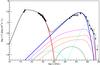 |
Fig. C.2 SED for PKS 2155-304 with a hadronic model with a magnetic field of log B [G] = 0.5 and an emission region of size log R [cm] = 16.5. |
 |
Fig. C.3 SED for PKS 2155-304 with a hadronic model with a magnetic field of log B [G] = 0.7 and an emission region of size log R [cm] = 16.2. |
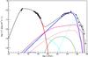 |
Fig. C.4 SED for PKS 2155-304 with a hadronic model with a magnetic field of log B [G] = 0.9 and an emission region of size log R [cm] = 15.9. |
 |
Fig. C.5 SED for PKS 2155-304 with a hadronic model with a magnetic field of log B [G] = 1.1 and an emission region of size log R [cm] = 15.5. |
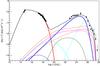 |
Fig. C.6 SED for PKS 2155-304 with a hadronic model with a magnetic field of log B [G] = 1.3 and an emission region of size log R [cm] = 15.3. |
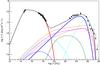 |
Fig. C.7 SED for PKS 2155-304 with a hadronic model with a magnetic field of log B [G] = 1.5 and an emission region of size log R [cm] = 15.0. |
 |
Fig. C.8 SED for PKS 2155-304 with a hadronic model with a magnetic field of log B [G] = 1.7 and an emission region of size log R [cm] = 14.7. |
 |
Fig. C.9 SED for PKS 2155-304 with a hadronic model with a magnetic field of log B [G] = 2.1 and an emission region of size log R [cm] = 14.2. |
Appendix D: selected models for Mrk 421
The following figures show all the hadronic models for Mrk 421 for an intermediate index of the proton spectrum n1 = 1.8 that passed our selection. The models for n1 = 1.7 and n1 = 1.9 are not included here for sake of brevity. Figure 2 contains the interpretation of the different curves.
 |
Fig. D.1 SED for Mrk 421 with a hadronic model with a magnetic field of log B [G] = 1.5 and an emission region of size log R [cm] = 14.7. |
 |
Fig. D.2 SED for Mrk 421 with a hadronic model with a magnetic field of log B [G] = 1.7 and an emission region of size log R [cm] = 14.5. |
 |
Fig. D.3 SED for Mrk 421 with a hadronic model with a magnetic field of log B [G] = 1.9 and an emission region of size log R [cm] = 14.2. |
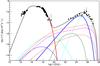 |
Fig. D.4 SED for Mrk 421 with a hadronic model with a magnetic field of log B [G] = 2.1 and an emission region of size log R [cm] = 14.1. |
All Figures
|
Fig. 1 Location of hadronic solutions in the log R-log B parameter plane. The frequency of the proton synchrotron emission peak remains constant along the dashed lines. The solid diagonal line separates the adiabatic cooling dominated domain from the radiative cooling dominated domain. The location of the typical solutions for HBLs shown in Figs. 2, 4 and 5 are indicated with markers and numbers. The dotted arrow points in the direction of decreasing proton synchrotron peak frequency. |
| In the text | |
|
Fig. 2 Variation in the modelled SED when moving along the diagonal in log R-log B space. From left to right, models with log B [G] = 0.5, 1.5, 2.0 are shown. Particle densities are adjusted to maintain the same overall flux level between the different models. Solid red and blue lines indicate the electron and proton synchrotron emission. The dotted and dashed lines show muon-synchrotron emission at the highest energies, and the SSC and muon-synchrotron cascade components at lower energies, as indicated in the legend. The VHE spectrum is absorbed by the EBL, assuming a redshift of 0.116, corresponding to the source PKS 2155-304. The spectral index n1 is chosen to be 1.9. The two dashed vertical lines are there to guide the eye by marking the approximate peak postitions of the model in the central figure. |
| In the text | |
|
Fig. 3 Location of hadronic solutions in log Lj-log η parameter space. The markers indicated the same solutions as shown in Fig. 1. The dashed curve represents the location of the proton-synchrotron solutions for a higher spectral index of the particle population. The vertical line marks equipartition between energy density of the magnetic field and relativistic protons. |
| In the text | |
|
Fig. 4 Variation in the modelled SED when varying R, i.e. moving along the red line in log R-log B space. From left to right, models with log R [cm] = 15.7, 15.3, and 15.0 are shown. Particle densities are adjusted to maintain the same overall flux level between the different models. Definition of the different curves as in Fig. 2. |
| In the text | |
|
Fig. 5 Variation in the modelled SED when varying B, i.e. moving along the blue line in log R-log B space. From left to right, models with log B [G] = 1.7, 1.5, 1.3 are shown. Particle densities are adjusted to maintain the same overall flux level between the different models. Definition of the different curves as in Fig. 2. |
| In the text | |
|
Fig. 6 SEDs for PKS 2155-304 with two hadronic models where proton synchrotron emission (left figure) or muon-synchrotron emission (right figure) dominates the TeV spectrum. These solutions correspond to a spectral index of n1 = 2.1 and 1.9, a magnetic field with log B [G] = 0.3 and 0.7, and an emission region of size log R [cm] = 9 × 10¹⁶ and 1.5 × 10¹⁶, respectively. See Fig. 2 for a description of the different curves. The dataset is described in the text. |
| In the text | |
|
Fig. 7 Source extension vs. magnetic field for HBL models. The different symbols correspond to the two different sources and to different spectral indices n1. The grey band indicates the range of values suggested for the Schwarzschild radius of PKS 2155-304, whereas the blue line shows the Schwarzschild radius of Mrk 421. |
| In the text | |
|
Fig. 8 Jet power vs. equipartition ratio for HBL models. The different symbols correspond to the two different sources and to different spectral indices n1. The grey band indicates the range of values suggested for the Eddington luminosity of PKS 2155-304, whereas the blue line shows the Eddington luminosity of Mrk 421. |
| In the text | |
|
Fig. 9 SEDs for Mrk 421 with two hadronic models where muon-synchrotron emission dominates the TeV spectrum. These solutions correspond to a spectral index n1 = 1.7 and 1.9, a magnetic field with log B [G] = 1.9 and 1.5, respectively, and an emission region of size log R [cm] = 1.5 × 10¹⁴ and 5.7 × 10¹⁴, respectively. See Fig. 2 for a description of the different curves. The dataset is described in the text. |
| In the text | |
|
Fig. 10 SEDs for PKS 2155-304 (left figure) and Mrk 421 (right figure) with an SSC model, where only electron synchrotron emission and SSC emission are considered. These solution correspond to a magnetic field with log B [G] = −1.4 and −1.1, and an emission region of size log R [cm] = 16.8 and 16.0, respectively. The solid red line corresponds to the electron-synchrotron emission and the dotted green line to the SSC component. The datasets are described in the text. |
| In the text | |
|
Fig. 11 Source extension vs. magnetic field for the UHBL models discussed by C15. The locations for the two different types of models are shown in black for the proton-synchrotron scenario and in red for the mixed lepto-hadronic scenario. The grey band indicates the range of Schwarzschild radii for the five UHBLs considered. |
| In the text | |
|
Fig. 12 Jet power vs. equipartition ratio for the UHBL models discussed by C15. The locations for the two different types of models are shown in black for the proton-synchrotron scenario and in red for the mixed lepto-hadronic scenario. The grey band indicates the range of Eddington luminosities for the UHBLs considered. |
| In the text | |
|
Fig. 13 Example of testing emission scenarios with CTA: comparison of the expected CTA spectra for two specific emission models for PKS 2155-304. A hadronic scenario is shown on the left, in which n1 = 2.1, log B [G] = 1.1. and log R [cm] = 15.6, and a standard leptonic SSC model on the right. The exposure time assumed for the simulations, 33 h, is the same as the live time for the H.E.S.S. observations, which are represented by grey data points above 3 × 1025 Hz. H.E.S.S. upper limits are not shown. Uncertainties in the CTA data points are smaller than the red squares. |
| In the text | |
|
Fig. 14 Example of a logparabolic fit to realisations of simulated spectra, upper panel, for an SSC model (black circles, upper fit parameters) and a hadronic model (red squares, lower fit parameters). The spectra correspond to a 50 h exposure time on the source PKS 2155-304. The lower panel shows the ratio of the simulated fluxes over the fit function. |
| In the text | |
|
Fig. 15 Mean values of the reduced χ2 distributions of logparabolic fits to one hundred realisations of each model for the SEDs of PKS 2155-304. The abscissa shows the logarithm of the magnetic field strength to distinguish different hadronic models. The error bars show the standard deviation of the distributions. The energy range of the fit was chosen to provide a good reduced χ2 for two different SSC models. The grey band is the union of the 1-σ envelopes of those SSC spectrum fits. |
| In the text | |
|
Fig. 16 Mean logarithmic values of the probabilities for the same fits as Fig. 15 for PKS 2155-304. The abscissa shows the logarithm of the magnetic field strength to distinguish different hadronic models. The error bars show the standard deviation of the distributions. The grey band is the union of the 1-σ envelopes of the SSC spectrum fits. |
| In the text | |
|
Fig. 17 Mean values of the reduced χ2 distributions of logparabolic fits to one hundred realisations of each model for the SEDs of Mrk 421. The caption of Fig. 15 contains more details. |
| In the text | |
|
Fig. 18 Mean logarithmic values of the probabilities for the same fits as Fig. 17 for Mrk 421. The abscissa shows the logarithm of the magnetic field strength to distinguish different hadronic models. The error bars show the standard deviation of the distributions. The grey band is the union of the 1-σ envelopes of the SSC spectrum fits. |
| In the text | |
|
Fig. 19 Expected neutrino spectra on Earth (all flavours combined) for two hadronic models for PKS 2155-304. “Model 1” has a small log B [G] = 0.3, whereas “Model 2” has a much larger log B [G] = 1.9. |
| In the text | |
|
Fig. 20 Expected neutrino spectra on Earth (all flavours combined) for two hadronic models for Mrk 421. “Model 1” has a log B [G] = 1.5, whereas “Model 2” has a log B [G] = 2.1. |
| In the text | |
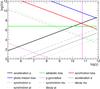 |
Fig. A.1 Relevant timescales for PKS 2155-304 for the model shown in Fig. 6 in the left panel. |
| In the text | |
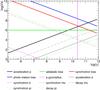 |
Fig. A.2 Relevant timescales for PKS 2155-304 for the model shown in Fig. 6 in the right panel. |
| In the text | |
|
Fig. B.1 Relevant timescales for Mrk 421 for the model shown in Fig. 9 in the left panel. For a description of the different lines, see Appendix A. |
| In the text | |
|
Fig. B.2 Relevant timescales for Mrk 421 for the model shown in Fig. 9 in the right panel. For a description of the different lines, see Appendix A. |
| In the text | |
|
Fig. C.1 SED for PKS 2155-304 with a hadronic model with a magnetic field of log B [G] = 0.3 and an emission region of size log R [cm] = 16.9. |
| In the text | |
|
Fig. C.2 SED for PKS 2155-304 with a hadronic model with a magnetic field of log B [G] = 0.5 and an emission region of size log R [cm] = 16.5. |
| In the text | |
|
Fig. C.3 SED for PKS 2155-304 with a hadronic model with a magnetic field of log B [G] = 0.7 and an emission region of size log R [cm] = 16.2. |
| In the text | |
|
Fig. C.4 SED for PKS 2155-304 with a hadronic model with a magnetic field of log B [G] = 0.9 and an emission region of size log R [cm] = 15.9. |
| In the text | |
|
Fig. C.5 SED for PKS 2155-304 with a hadronic model with a magnetic field of log B [G] = 1.1 and an emission region of size log R [cm] = 15.5. |
| In the text | |
|
Fig. C.6 SED for PKS 2155-304 with a hadronic model with a magnetic field of log B [G] = 1.3 and an emission region of size log R [cm] = 15.3. |
| In the text | |
|
Fig. C.7 SED for PKS 2155-304 with a hadronic model with a magnetic field of log B [G] = 1.5 and an emission region of size log R [cm] = 15.0. |
| In the text | |
|
Fig. C.8 SED for PKS 2155-304 with a hadronic model with a magnetic field of log B [G] = 1.7 and an emission region of size log R [cm] = 14.7. |
| In the text | |
|
Fig. C.9 SED for PKS 2155-304 with a hadronic model with a magnetic field of log B [G] = 2.1 and an emission region of size log R [cm] = 14.2. |
| In the text | |
|
Fig. D.1 SED for Mrk 421 with a hadronic model with a magnetic field of log B [G] = 1.5 and an emission region of size log R [cm] = 14.7. |
| In the text | |
|
Fig. D.2 SED for Mrk 421 with a hadronic model with a magnetic field of log B [G] = 1.7 and an emission region of size log R [cm] = 14.5. |
| In the text | |
|
Fig. D.3 SED for Mrk 421 with a hadronic model with a magnetic field of log B [G] = 1.9 and an emission region of size log R [cm] = 14.2. |
| In the text | |
|
Fig. D.4 SED for Mrk 421 with a hadronic model with a magnetic field of log B [G] = 2.1 and an emission region of size log R [cm] = 14.1. |
| In the text | |
Current usage metrics show cumulative count of Article Views (full-text article views including HTML views, PDF and ePub downloads, according to the available data) and Abstracts Views on Vision4Press platform.
Data correspond to usage on the plateform after 2015. The current usage metrics is available 48-96 hours after online publication and is updated daily on week days.
Initial download of the metrics may take a while.