| Issue |
A&A
Volume 602, June 2017
|
|
|---|---|---|
| Article Number | A111 | |
| Number of page(s) | 15 | |
| Section | Numerical methods and codes | |
| DOI | https://doi.org/10.1051/0004-6361/201629507 | |
| Published online | 23 June 2017 | |
LSDCat: Detection and cataloguing of emission-line sources in integral-field spectroscopy datacubes⋆
1 Leibniz-Institut für Astrophysik Potsdam (AIP), An der Sternware 16, 14482 Potsdam, Germany
e-mail: This email address is being protected from spambots. You need JavaScript enabled to view it.
2 Department of Astronomy, Stockholm University, AlbaNova University Centre, 106 91 Stockholm, Sweden
Received: 9 August 2016
Accepted: 15 March 2017
Abstract
We present a robust, efficient, and user-friendly algorithm for detecting faint emission-line sources in large integral-field spectroscopic datacubes together with the public release of the software package Line Source Detection and Cataloguing (LSDCat). LSDCat uses a three-dimensional matched filter approach, combined with thresholding in signal-to-noise, to build a catalogue of individual line detections. In a second pass, the detected lines are grouped into distinct objects, and positions, spatial extents, and fluxes of the detected lines are determined. LSDCat requires only a small number of input parameters, and we provide guidelines for choosing appropriate values. The software is coded in Python and capable of processing very large datacubes in a short time. We verify the implementation with a source insertion and recovery experiment utilising a real datacube taken with the MUSE instrument at the ESO Very Large Telescope.
Key words: methods: data analysis / techniques: imaging spectroscopy
The LSDCat software is available for download at http://muse-vlt.eu/science/tools and via the Astrophysics Source Code Library at http://ascl.net/1612.002
© ESO, 2017
1. Introduction
One motivating driver for the construction of the current generation of optical wide-area integral-field spectrographs such as the Multi Unit Spectroscopic Explorer at the ESO VLT (MUSE, in operation since 2014; Bacon et al. 2014; Kelz et al. 2016) or the Keck Cosmic Web Imager (KCWI, under construction; Martin et al. 2010) is the detection of faint emission lines from high-redshift galaxies. The high-level data products from those instruments are three-dimensional (3D) arrays containing intensity-related values with two spatial axes and one wavelength axis (usually referred to as datacubes). So far, efficient, robust, and user-friendly detection and cataloguing software for faint-line-emitting sources in such datacubes is not publicly available. To remedy this situation we now present the Line Source Detection and Cataloguing (LSDCat) tool, developed in the course of our work within the MUSE consortium.
Automatic source detection in two-dimensional (2D) imaging data is a well-studied problem. Various methods to tackle it have been implemented in software packages that are widely adopted in the astronomical community (see reviews by Bertin 2001; and Masias et al. 2012, or the comparison of two frequently used tools by Annunziatella et al. 2013). A conceptually simple approach consists of two steps: first, the observed imaging data is transformed in order to highlight objects while simultaneously reducing the background noise. A particular transformation that satisfies both requirements is the matched filter (MF) transform. Here the image is cross-correlated with a 2D template that matches the expected light distribution of the sources to be detected. Mathematically, it can be proven that for stationary noise the MF maximises the signal-to-noise ratio (S/N) of a source that is optimally represented by the template (e.g. Schwartz & Shaw 1975; Das 1991; Zackay & Ofek 2017; Vio & Andreani 2016). In the second step, the MF-transformed image is segmented into objects via thresholding, that is, each pixel in the threshold mask is set to 1 if the MF-transformed value is above the threshold, and 0 otherwise. Connected 1-valued pixels then define the objects on which further measurements (e.g. centroid coordinates, brightnesses, ellipticities etc.) can be performed. Other image transformations (e.g. multi-scale methods) and detection strategies (e.g. histogram-based methods) exist, but the “MF + thresholding”-approach is most frequently employed, especially in optical/near-infrared imaging surveys for faint extragalactic objects. This widespread preference is certainly attributable to the conceptual simplicity and robustness of the method, despite known limitations (see e.g. Akhlaghi & Ichikawa 2015). But it is also due to the availability of a stable and user-friendly implementation of a software based on this approach (Shore 2009): SExtractor (Bertin & Arnouts 1996).
The detection and cataloguing of astronomical sources in 3D datasets has so far mostly been of interest in the domain of radio astronomy. Similar to integral-field spectroscopy (IFS), these observations result in 3D datacubes containing intensity values with two spatial axes and one frequency axis. Here, especially surveys for extragalactic 21 cm H i emission are faced with the challenge to discover faint line emission-only sources in such datacubes. The current generation of such surveys utilises a variety of custom-made software for this task, also relying heavily on manual inspection of the datacubes. Notably, the approach of Saintonge (2007) tries to minimise such error-prone interactivity by employing a search technique based on matched filtering, although only in spectral direction. More recently, driven mainly by the huge data volumes expected from future generations of large radio surveys with the Square Kilometre Array, development and testing of new 3D source-finding techniques has started (e.g. Koribalski 2012; Popping et al. 2012; Serra et al. 2012; Jurek 2012). Currently, two software packages implementing some of these techniques are available to the community: duchamp (Whiting 2012) and SoFiA (Serra et al. 2015). While in principle these programs could be adopted for source detection purposes in optical integral-field spectroscopic datasets, in practice there are limitations that necessitate the development of a dedicated IFS source detector. For example, the noise properties of long exposure IFS datacubes are dominated by telluric line- and continuum emission and are therefore varying with wavelength, in contrast to the more uniform noise properties of radio datacubes. Moreover, the search strategies implemented in the radio 3D source finders are tuned to capture the large variety of signals expected. But, as we argue in this paper, the emission line signature from compact high-redshift sources in IFS data is well described by a simple template that, however, needs an IFS-specific parameterisation. Finally, the input data as well as the parameterisation of detected sources is different in the radio domain compared to the requirements in optical IFS: typically radio datacubes have their spectral axis expressed as frequency and flux densities measured in Jansky, while in IFS cubes the spectral axis is in wavelengths and flux densities are measured as fλ with units of erg s-1 cm-2 Å-1.
LSDCat is part of a long-term effort, initially motivated by the construction of MUSE, to develop source detection algorithms for wide-field IFS datasets (e.g. Bourguignon et al. 2012). As part of this effort, Meillier et al. (2016) recently released the Source Emission Line FInder (SELFI). This software is based on a Baysian scheme utilising a reversible jump Monte Carlo Markov chain algorithm. While this mathematically sophisticated machinery is quite powerful in unearthing faint emission line objects in a datacube, the execution time of the software is too long for practical use. In contrast, the algorithm of LSDCat is relatively simple and correspondingly fast in execution time on state-of-the art workstations. It is also robust, as it is based on the matched-filtering method that has long been successfully utilised for detecting sources in imaging data. LSDCat is therefore well suited for surveys exploiting even large numbers of wide-field IFS datacubes. Furthermore, the short execution time also permits extensive fake source insertion experiments to empirically reconstruct the selection function of such surveys.
This article is structured as follows: in Sect. 2, we describe the mathematical basis and the algorithm implemented in LSDCat. In Sect. 3, we validate the correctness of the implementation in our software. We then provide guidelines for the LSDCat user for adjusting the free parameters governing the detection procedure in Sect. 4 and conclude in Sect. 5 with a brief outlook on future improvements of LSDCat. A link to the software repository is available from the Astrophysics Source Code Libary1. In Appendix A, we provide a short example on how the user interacts with LSDCat routines. The public release of the software includes a detailed manual, to which we refer all potential users for details of installing and working with the software.
Routines of LSDCat with the required input parameters.
2. Method description and implementation
2.1. Input data
The principal data product of an integral field unit (IFU) observing campaign is a datacube F (e.g. Allington-Smith 2006; Turner 2010). The purpose of LSDCat is to detect and characterise emission-line sources in F. We adopt the following notations and conventions: F is a set of volume pixels (voxels) Fx,y,z with intensity related values, for example, flux densities in units of erg s-1 cm-2 Å-1. The indices x,y index the spatial pixels (spaxels), and z indexes the spectral layers of the datacube. Mappings between x,y and sky position (right ascension and declination), as well as between z and wavelength λ can be included in the metadata (Greisen & Calabretta 2002; Greisen et al. 2006). For the new generation of wide-field IFUs based on image-slicers, the sky is sampled contiguously, and typical dimensions of a MUSE datacube are xmax,ymax,zmax ≃ 3 × 102,3 × 102,4 × 103, that is, a datacube consists of ~ 4 × 10⁸ voxels.
We make a number of assumptions regarding the data structure, guided by the output of the MUSE data reduction system (DRS; Weilbacher et al. 2012, 2014):
-
We assume that atmospheric line and continuum emission hasbeen subtracted from F (Streicher et al. 2011; Soto et al. 2016); see Sect. 4.4 for a brief discussion on how to account for sky subtraction residuals within LSDCat.
-
LSDCat currently requires a rectilinear grid in x,y,z. In particular, the mapping between z and λ has to be linear with a fixed increment Δλ per spectral layer, that is,
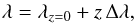 (1)where λz = 0 designates the wavelength corresponding to the wavelength of the first spectral layer. For MUSE, this is achieved by the DRS through resampling the raw CCD data into the final datacube F. We also demand a constant mapping between x,y and sky position for all spectral layers z, which the MUSE pipeline accounts for in the resampling step by correcting for the wavelength-dependent lateral offset (differential atmospheric refraction) along the parallactic angle (e.g. Filippenko 1982; Roth 2006).
 -
Together with the flux datacube F, LSDCat expects a second cube σ2 containing voxel-by-voxel variances. While such a variance cube is provided by the MUSE DRS as formal propagation of the various detector-level noise terms through the data reduction steps, the pipeline currently neglects the covariances between adjacent voxels introduced by the resampling process. We discuss this issue and some practical considerations further in Sect. 4.4; here we simply assume that a datacube σ2 with appropriate variance estimates is available.
As a very useful preparatory step for LSDCat, we recommend that galaxies and stars with bright continuum emission (i.e. sources with significant signal in the majority of spectral bins) are subtracted from F. While the presence of such sources does not render the detection and cataloguing algorithm unusable, continuum bright sources may lead to (possibly many) catalogue entries unrelated to actual emission-line objects. We give some guidance for the subtraction of continuum bright sources prior to running LSDCat in Sect. 4.1.
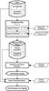 |
Fig. 1 Flowchart illustrating the processing steps of LSDCat from an input datacube to a catalogue of positions, shape parameters, and fluxes of emission line sources. |
Figure 1 depicts, as a flowchart, all the main processing steps of LSDCat, leading from the input datacube F and its associated variances σ2 to a catalogue of emission lines. Each processing step is implemented as a stand-alone Python2 program. The file format of the input data and variance cubes has to conform to the FITS standard (Pence et al. 2010). LSDCat requires routines provided by NumPy3 (van der Walt et al. 2011), SciPy4 (Jones et al. 2001), and Astropy5 (Astropy Collaboration et al. 2013). For performing its operations, LSDCat needs up to four datacubes loaded simultaneously. Hence, for typical MUSE datacubes that contain ~ 108 − 109 32-bit floating point numbers, a computer with at least 16 GB of random access memory is recommended. Table 1 lists the names of the individual LSDCat routines implementing the various processing steps, together with the main input parameters that govern the detection and cataloguing process. In the following we describe each of the processing steps with its routines in more detail. A practical example of using the LSDCat routines is provided in Appendix A.
2.2. 3D matched filtering
The optimal detection statistic of an isolated signal in a dataset with additive white Gaussian noise is given by the matched filter transform of the dataset (e.g. Schwartz & Shaw 1975; Das 1991; Bertin 2001; Zackay & Ofek 2017; Vio & Andreani 2016). This transform cross-correlates the dataset with a template that matches the properties of the signal to be detected.
We utilise the matched filtering approach in LSDCat to obtain a robust detection statistic for isolated emission line sources in wide-field IFS datacubes. For a symmetric 3D template T, this is equivalent to a convolution of F with T:  (2)Here ∗ denotes the (discrete) convolution operation, that is, every voxel of
  is given by
  (3)In principle, the summation runs over all dimensions of the datacube, but in practice, terms where Ti,j,k ≈ 0 can be neglected. Propagating the variances from σ2 through Eq. (3) yields the voxels of
  :
:  (4)The template T must be chosen such that its spectral and spatial properties match those of a compact expected emission-line source in F. LSDCat is primarily intended to search for faint compact emission-line sources. For such sources it is a reasonable assumption that their spatial and spectral properties are independent of one another. We can therefore write T as a product
  (5)where Tspat is the expected spatial profile and Tspec is the expected spectral profile. The voxels of T are thus given by
  (6)Of course, spatially extended sources with a velocity profile along the line of sight are not optimally captured by separating the filter into the spectral and spatial domain. However, as we detail in Sects. 4.2 and 4.3, moderate template mismatches do not result in a major reduction of the maximum detectability that could be achieved with an exactly matching template.
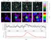 |
Fig. 2 Example of the effect of matched filtering on the detectability of a faint emission-line source in the MUSE datacube of the Hubble Deep Field South (Bacon et al. 2015). Shown is a Lyman α emitting galaxy at redshift z = 3.278 with flux FLyα = 1.3 × 10⁻¹⁸ erg s-1 (ID #162 in Bacon et al. 2015). The panels in the first row display four different spectral layers of the continuum-subtracted datacube F. The second row shows the same spectral layers, but for the filtered S / N cube (Eq. (9)) that was used to build the catalogue of emission line sources via thresholding (Eq. (18)). The leftmost panels show a layer significantly away from the emission line peak, the other panels show layers at spectral coordinates zpeak − 1, zpeak, and zpeak + 1, respectively, where zpeak designates the layer containing the maximum S / N value of the source. The third row shows the flux density spectrum in the spaxels at (xpeak,ypeak) and (xpeak ± 1,ypeak ± 1), where xpeak and ypeak are the spatial coordinates of the highest S/N value. The bottom row shows a S/N spectrum extracted from the S / N cube at xpeak and ypeak. |
Now with Eq. (6), the 3D convolution of Eq. (3) yielding can be performed as a succession of two separate convolutions, in no particular order: a spatial convolution with the appropriate Tspat in each spectral layer z, and a spectral convolution with Tspec in each spaxel x,y:  Note that since every spectral layer z of the datacube is convolved with a different spatial template, and since the width of the spectral template also changes with z (see Sect. 2.3), the equivalence between Eqs. (7) and (8), mathematically speaking, is not strictly correct. However, the variations of the templates with λ are much slower than the typical line widths of the spectral templates, meaning that we can approximate the convolution by using a locally invariant template.
As an indicator of the presence or absence of an emission line in F at a position x,y,z we then evaluate the statistic  (9)with
  from Eq. (3) and
  as the square root of Eq. (4). The voxels S / Nx,y,z constitute the signal-to-noise cube
  (10)computed after the matched filtering has been performed. The values on the left side of Eq. (9) can be translated into a probability for rejecting the null-hypothesis of no source being present at position x,y,z in F. This is commonly referred to as the detection significance of a source. However, in a strict mathematical sense this direct translation is only valid for sources that are exactly described by the adopted template T, in a dataset where the variance terms on the right-hand side of Eq. (4) are stationary and fully uncorrelated. Nevertheless, even if these strict requirements are not met by the IFS datacube, filtering with T will always reduce high-frequency noise while enhancing the presence of sources that are similar in appearance with T. Thus Eq. (9) can still be used as a robust empirical measure of the significance of a source present in F at a position x,y,z. We illustrate this for a faint high-redshift Lyman α-emitting galaxy observed with MUSE in Fig. 2; this source is detected with high significance at a peak S / N value of ~9 in the S / N-cube, although it is barely visible in the monochromatic layers of the original MUSE datacube.
In LSDCat, the spatial convolution is performed by the routine lsd_cc_spatial.py and the spectral convolution is performed by lsd_cc_spectral.py. The output of a subsequent run of those routines is a FITS file with two header and data units; one storing and the other one storing . Both routines are capable of fully leveraging multiple processor cores, if available, to process several datacube layers or spaxels simultaneously. Moreover, in lsd_cc_spatial.py the computational time is reduced by using the fast Fourier transform method provided by SciPy to convolve the individual layers. However, since the spectral kernel varies with wavelength we cannot utilise the same approach in lsd_cc_spectral.py, but the discrete 1D convolution operation can be written as a matrix-vector product with the convolution kernel given by a sparse banded matrix (Das 1991, Sect. 3.3.6). Hence here we achieve a substantial acceleration of the computational speed by utilising the sparse matrix multiplication algorithm of SciPy. Typical execution times of lsd_cc_spatial.py and lsd_cc_spectral.py running in sequence on a full MUSE 300 × 300 × 4000 datacube, including reading and writing of the data, are ~ 5 min on an Intel Core-i7 workstation with 8 cores, or ~ 2 min on a workstation with two AMD Opteron 6376 processors with 32 cores each.
2.3. Templates
In line with the approximate separation of spatial and spectral filtering described in the previous subsection, LSDCat requires two templates, a spatial and a spectral one.
For the spatial template Tspat the user has currently the choice between a circular Gaussian profile,  (11)with the standard deviation σG, or a Moffat (1969) profile,
 ![Mathematical equation: \begin{equation} \label{lsd_eq:9} T_{x,y} = \frac{\beta - 1}{\pi r_\mathrm{d}^2} \left [ 1 + \frac{x^2 + y^2}{r_\mathrm{d}^2} \right ]^{-\beta} \text{,} \end{equation}](/articles/aa/full_html/2017/06/aa29507-16/aa29507-16-eq64.png) (12)with the width parameter rd and the kurtosis parameter β. Both functions6 are commonly used as approximation of the seeing induced point spread function (PSF) in ground-based optical and near-IR observations (Trujillo et al. 2001a,b) and therefore are well suited as spatial templates for compact emission line sources. Of course it is also possible to adopt a spatial template more extended than the PSF by choosing a correspondingly large value of σG or rd. As discussed in Sects. 4.2 and 4.3 below, the maximum S / N delivered by the matched filter behaves very benignly with respect to modest template mismatch, and the application of LSDCat is thus by no means limited to search for point sources.
(12)with the width parameter rd and the kurtosis parameter β. Both functions6 are commonly used as approximation of the seeing induced point spread function (PSF) in ground-based optical and near-IR observations (Trujillo et al. 2001a,b) and therefore are well suited as spatial templates for compact emission line sources. Of course it is also possible to adopt a spatial template more extended than the PSF by choosing a correspondingly large value of σG or rd. As discussed in Sects. 4.2 and 4.3 below, the maximum S / N delivered by the matched filter behaves very benignly with respect to modest template mismatch, and the application of LSDCat is thus by no means limited to search for point sources.
Typically the parameter used to characterise the atmospheric seeing is the full width at half maximum (FWHM) of the PSF. For Eq. (11) this is  (13)and for the Moffat in Eq. (12) it is
  (14)Generally, the seeing depends on wavelength. Specifically, in MUSE data and adopting the Moffat form to describe the PSF, the variation of FWHM with λ appears to be mainly driven by rd, while β appears to be close to constant (e.g., Husser et al. 2016). In LSDCat we approximate the FWHM(λ) dependency as a quadratic polynomial
 ![Mathematical equation: \begin{equation} {\it FWHM}(\lambda)[\text{\arcsec}] = p_0 + p_1(\lambda - \lambda_0) + p_2 (\lambda - \lambda_0)^2 \label{eq:2} \text{,} \end{equation}](/articles/aa/full_html/2017/06/aa29507-16/aa29507-16-eq69.png) (15)where the coefficients p0[′′], p1[′′/Å], p2[′′/Å2], and the reference wavelength λ0 are input parameters supplied by the user. In Sect. 4.2 we further discuss the adopted PSF parametrisation and the choice of suitable parameter values.
(15)where the coefficients p0[′′], p1[′′/Å], p2[′′/Å2], and the reference wavelength λ0 are input parameters supplied by the user. In Sect. 4.2 we further discuss the adopted PSF parametrisation and the choice of suitable parameter values.
As a spectral template in LSDCat we employ a simple 1D Gaussian  (16)with the standard deviation σz. While the line profiles of actual galaxies may deviate in detail from this idealised function, the deviations are usually minor and do not lead to significant changes in the S / N achieved by the matched filter when compared to a simple Gaussian.
Since velocity broadening usually dominated the widths of emission lines from galaxies, LSDCat assumes the width of the spectral template to be fixed in velocity space, σv = const. As long as the mapping between λ and spectral coordinate z is linear, σz in Eq. (16) depends linearly on z when parameterised by σv:  (17)The input parameter supplied by the LSDCat user is the velocity FWHM of the Gaussian profile FWHMv = 2
 . In Sect. 4.3 we show that the S / N of any given emission line does not depend very sensitively on the chosen value of FWHMv, and in many cases a single spectral template with a typical value of FWHMv may be sufficient.
Output parameters for each LSDCat detection.
2.4. Thresholding
A catalogue of emission line sources can now be constructed by thresholding the S / N-cube with a user-specified value S / Ndet.. This threshold is used to create a binary cube L with voxels given by  (18)The detection threshold S / Ndet is the principal input parameter to be set by the LSDCat user. Each cluster of non-zero neighbouring voxels in L (6-connected topology) constitutes a detection. A high threshold will lead to a small number of highly significant detections, while lower values of S / Ndet will lead to more entries in the catalogue, but also increase the chance of including entries that are spurious, that is, that do not correspond to real emission line objects. We give guidelines on the choice of the detection threshold based on our experience with MUSE data in Sect. 4 below.
For each detection, LSDCat records the coordinates xpeak, ypeak,zpeak of the local maximum in the S / N-cube, its value S / Npeak ≡ S / Nxpeak,ypeak,zpeak, and the number of voxels Ndet constituting the detection. These values constitute an intermediate catalogue of detections. Each entry is assigned a unique running integer number i. Moreover, LSDCat also assigns an integer object identifier jObj to detection clusters occurring at different wavelengths but similar spatial positions within a small search radius to account for sources with multiple significantly detectable emission lines. This intermediate catalogue is created by the routine lsd_cat.py, utilising routines from the SciPy ndimage.measurements package. The intermediate catalogue is written to disk as a FITS binary table. The actual execution time is generally much shorter than the previous step of applying the matched filter, but it depends on the detection threshold that determines the number of objects.
2.5. Measurements
LSDCat provides a set of basic measurement parameters for each detection of the intermediate catalogue. These parameters are determined using the datacubes F, σ2, and S / N. The set of parameters is chosen to be robust and independent from a specific scientific application. For more complex measurements involving, for example, fitting of flux distributions, the LSDCat measurement capability can serve as a starting point.
In Table 2 we list the various output parameters that are generated for each detection. This parametrisation of the detected sources and their emission lines constitutes the final processing step of LSDCat. The routine lsd_cat_measure.py performs the parameterisation task and writes out the final catalogue. Running lsd_cat_measure.py on an intermediate catalogue with ~ 102 entries takes typically 100 s on the two machines mentioned above in Sect. 2.2, with most of the time spent on reading the four input datacubes.
2.5.1. Centroids
The coordinates of each detections local maximum in the S / N-cube (Sect. 2.4) serve only as a first approximation of its spatial and spectral position. As a refinement lsd_cat_measure.py can calculate several different sets of centroid positions for each detected line cluster. For example, the 3D S / N-weighted centroid is given by the first moments 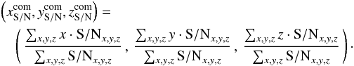 (19)Here, for each detection, the summation runs over all non-zero (xpeak, ypeak,zpeak)-neighbouring voxels in a thresholded datacube similar to L (Eq. (18)), but with voxels set to one if they are above an analysis threshold S / Nana. This additional threshold, which must be smaller or equal to S / Ndet, is the required input parameter for lsd_cat_measure.py. Guidelines for choosing S / Nana are discussed in Sect. 4.5. Similarly, LSDCat can measure 3D centroid coordinates with the original flux cube F and with the filtered flux cube as weights. In these cases, Eq. (19) is applied again, but with S / Nx,y,z being substituted by Fx,y,z and , respectively.
3D centroids provide a non-parametric way of calculating spatial and spectral positions, making use of the full 3D information present in the datacube. While the calculation using the flux cube is unbiased against a particular choice of filter template, it is not very robust for low S / N detections. This shortcoming is alleviated for the centroids calculated on the filtered flux cube or the S / N-cube. The latter, however, could potentially be biased by local noise extrema, for example, at spectral layers near sky-lines.
As an alternative approach to 3D centroids, LSDCat can calculate 2D centroids on synthesised narrow-band images  from the filtered flux cube :
  (20)The boundary indices of each synthetic narrowband image
  and
and  are taken as the minimum and maximum z coordinate of all voxels of a detection above the analysis threshold S / Nana. Then the 2D weighted centroid coordinates follow from the first image moments:
 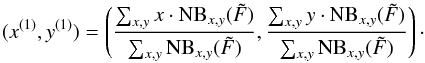 (21)In this equation the summation runs over all pixels x,y of that belong to the detection cluster and are above the analysis threshold S / Nana in the zpeak layer of the S / N-cube.
The 2D narrowband images are furthermore used by lsd_cat_measure.py to derive basic shape information using the second central image moments of each detection. These are defined as ![Mathematical equation: \begin{eqnarray} \label{lsd_eq:17} x^{(2)} &=& \frac{\sum_{x,y} x^2 \cdot \mathrm{NB}_{x,y}(\tilde{F})}{\sum_{x,y} \mathrm{NB}_{x,y}(\tilde{F})} - (x^{(1)})^2 \text{,}\\ \label{lsd_eq:18} y^{(2)} &=& \frac{\sum_{x,y} y^2 \cdot \mathrm{NB}_{x,y}(\tilde{F})}{\sum_{x,y} \mathrm{NB}_{x,y}(\tilde{F})} - (y^{(1)})^2 \text{,}\\ \label{lsd_eq:19} {[xy]}^{(2)} &=& \frac{\sum_{x,y} x^2 \cdot y^2 \cdot \mathrm{NB}_{x,y}(\tilde{F})}{\sum_{x,y} \mathrm{NB}_{x,y}(\tilde{F})} - x^{(1)} \cdot y^{(1)} \text{.} \end{eqnarray}](/articles/aa/full_html/2017/06/aa29507-16/aa29507-16-eq130.png) These values are simple indicators for the spatial extent and elongation of a detected emission line cluster. For example, [ xy ] (2) ≡ 0 for a circular symmetric distribution of the object in . Moreover, in this case the radius
These values are simple indicators for the spatial extent and elongation of a detected emission line cluster. For example, [ xy ] (2) ≡ 0 for a circular symmetric distribution of the object in . Moreover, in this case the radius 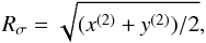 (25)encircles 68% of the flux in the filtered narrowband image for a perfect point source blurred by a Gaussian PSF.
While in principle, the original flux datacube F could also be used in Eqs. (20) to (24), in practice, the calculation of the moments directly from the flux cube is relatively susceptible to noise for very faint sources. Our experience with MUSE data showed that the centroids and shapes determined in the 2D narrowband images based on the filtered datacubes provide the most reliable measurements even for low S / N detections. Moreover, the spatial coordinates from Eq. (21) are in closest agreement with the centroids determined in broad-band imaging data.
2.5.2. Integrated line fluxes
The difficulty in measuring the total flux of a detected line lies in its unknown spectral shape and in the unknown spatial distribution of the flux. While for the detection it is not required to accurately know these properties (as long as the template mismatch is not too poor), the template scaling factor depends very critically on the degree of similarity between source and template and can therefore not be used as flux indicator. This is different from PSF matching techniques in stellar fields (e.g. Kamann et al. 2013), where all objects are point sources and no strong mismatches are expected. The task for LSDCat is different: We have to define 3D boundaries for each emission line to allow for the summation of voxel values within these boundaries as flux measurement, but avoid the inclusion of too many unrelated empty-sky voxels that would compromise the precision of the measurement. In line with the prime purpose of LSDCat as a detection tool, we implemented an approach that emphasises robustness over sophistication.
LSDCat addresses this task in two steps. The first is the construction of a narrowband image via setting an analysis S / N threshold as described in the previous subsection. A reasonable choice of S / Nana should produce spectral boundaries and that enclose the emission line (more or less) completely in the original datacube F. Therefore the pixels of the narrow-band image NBx,y(F) created by summation of F from to (analogous to Eq. (20)) can be used for flux integration.
The second step is then to derive suitable apertures for these narrowband images, taking the spatial extent of each source into account. Currently, LSDCat measures fluxes in circular apertures with radii defined as multiples k of the Kron radius (Kron 1980) of a detected line. The Kron radius is however determined not in the measured dataset itself, but again in the narrowband image based on the filtered datacube, which makes the procedure much more robust especially at low S/N. The measured quantity is then F(k·RKron) with 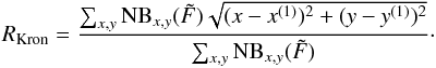 (26)In order to avoid possibly unphysically small or large values of RKron caused by artefacts in the data, a minimal and a maximal value for RKron can be set by the user.
The factor k is also defined by the LSDCat user. Multiple values of k result in multiple columns of the output catalogue. The line flux Fline(k·RKron) is then given by the sum 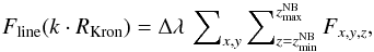 (27)with the first sum running over all x,y that satisfy
  . The aperture thus has cylindrical shape, with its symmetry axis going through the 2D centroid position. The factor Δλ that denotes the increment per spectral layer is needed to convert the sum of voxel values into a proper integral over the line.
It can be shown that the 2.5 RKron aperture includes ≳90% of the total flux even for extended sources with relatively shallow profiles, as long as the determination of the Kron radius in Eq. (26) accounts for pixels at sufficiently large radii (Graham & Driver 2005). We follow a similar approach as adopted in SExtractor (Bertin & Arnouts 1996) by summing over all x,y in Eq. (26) that satisfy  (28)with Rσ as defined in Eq. (25). The uncertainty σF of this flux measurement is obtained by propagating the voxel variances
  through Eq. (27).
3. Validation of the software
3.1. Creation of test datacubes
We now validate the correctness of the algorithms implemented in the LSDCat software. To this aim we produced a set of datacubes that contain fake emission line sources at known positions with known fluxes and extents. Instead of utilising a completely artificial data set with ideal noise, we based our source insertion experiment on the MUSE HDFS datacube7 (Bacon et al. 2015). Thereby we ensure that our test data is identical in noise (and potential systematics) with real observations. Furthermore, we self-calibrated the noise by calculating empirical variances as we recommend in Sect. 4.4.
We implanted the fake emission line sources into a continuum-subtracted version of the HDF-S datacube at a wavelength of 5000 Å. Continuum subtraction was performed with the median-filter subtraction method detailed in Sect. 4.1. The chosen insertion wavelength ensures a clean test environment that is not hampered by systematic sky-subtraction residuals which exist in the redder parts of the datacube. In total we created 23 test datacubes for the fake source emission line fluxes log F [ erg s-1 cm-2 ] = − 16.2 to − 18.5 in steps of 0.1 dex. Each cube contains 51 fake sources with the same emission line flux. The spatial positions of the implanted sources are based on the pseudo-random Sobol sequence (Press et al. 1992, Sect. 7.7). The pseudo-random grid guarantees that all sources have different distances to the edges of the rectangular grid of MUSE slicer-stacks, thus possible systematic effects from localised noise properties within this slicer-stack grid are mitigated. As test sources we utilised Gaussian emission lines with a line width (FWHM) of 250 km s-1. The sources were assumed to be PSF-like and we approximated the PSF blurring by a 2D Gaussian with 0.88′′ FWHM at 5000 Å, a value we obtained from a 2D Gaussian fit to the brightest star in the HDFS field. The datacubes containing the fake sources as well as all processing steps needed to reproduce the results from the validation exercise presented in this section are available via the LSDCat software repository.
3.2. Minimum detectable emission line flux at a given detection threshold
For known background noise, the minimum detection significance at which an emission line can be recovered from the datacube is intrinsically linked to the total flux of the line, its spatial and spectral morphology, and the degree of mismatch between filter template and emission line source signal. The latter we discuss in Sects. 4.2 and 4.3 for the spectral and spatial filtering processes, respectively, and Gaussian emission line expressions for the detection significance attenuation due to shape mismatch are presented in Eqs. (36) and (37).
For the test datacubes described above we have complete control over the shape parameters. Thus we can use the exact template in the matched filtering process. As a benchmark we will now derive an analytic approximation for the minimum recoverable line flux at a given detection threshold and then compare the result to a source recovery experiment performed with LSDCat on the test datacube.
For the match between emission line and filter being perfect in the datacube, the flux distribution of that emission line at position x′,y′,z′ in the datacube can be written as 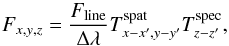 (29)with Fline being the total flux in that line, Δλ being the wavelength increment per spectral layer defined in Eq. (1), and
  and
and  being the spectral and spatial templates given by Eqs. (16) and (11) for the 1D and 2D Gaussian, respectively. With Eqs. (29) and (8), we can thus write for the peak value of the matched filtered datacube at position x′,y′,z′:
 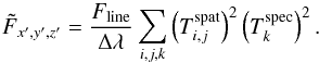 (30)Since the noise is usually not constant over the shape of the filter, there exists no general solution for the error propagation given in Eq. (4). To obtain an approximate solution, we approximate σx,y,z as being, on average, constant spectrally and spatially, at least over all voxels within the matched filter:
  . Due to the absence of strong sky emission lines in the blue part of the MUSE datacube this approximation is well justified for the test data set that we consider here. Therefore Eq. (4) can be written as
 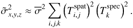 (31)Assuming that the dispersion σZ and σG of the 1D and 2D Gaussian in Eqs. (11) and (21) are large enough to make sampling and aliasing effects of the profiles in the datacube negligible we can replace the sum with an integral, thus
  (32)and
  (33)With these expressions in Eqs. (30) and (31) we can write the peak detection significance of the line at position x′,y′,z′ via Eq. (9) as
  (34)With the expression given in Eq. (34) it is now possible to estimate the minimum recoverable line flux at a given detection threshold. For the artificial sources implanted in the MUSE HDFS data we have σG = 0.88″ = 1.84 px. The spectral line width vFWHM = 250 km s-1 translates to σz = 1.46 px at 5000 Å and Δλ = 1.2 Å. By averaging our empirical noise estimate around 5000 Å we find
  erg s-1 cm-2 Å-1. As we detail in Sect. 4.5 for the MUSE HDFS datacube, a detection threshold of S / Ndet ≈ 8 is a value found to be suitable for practical work. With the stated values inserted into Eq. (34) we calculate
 ![Mathematical equation: \begin{equation} \label{eq:10} \log F_\mathrm{line} \;[\mathrm{erg\,s^{-1}\,cm^{-2}}] \approx -17.83 \end{equation}](/articles/aa/full_html/2017/06/aa29507-16/aa29507-16-eq168.png) (35)as the minimum line flux at which sources should be detectable at S / Ndet = 8, if an exactly matching filter was chosen in the cross-correlation process.
(35)as the minimum line flux at which sources should be detectable at S / Ndet = 8, if an exactly matching filter was chosen in the cross-correlation process.
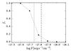 |
Fig. 3 Completeness curve |
We now perform the recovery experiment utilising the test datacubes introduced in Sect. 3.1 to check whether LSDCat is indeed able to detect emission line sources with S / Ndet = 8 at the estimated minimum line flux. Therefore we process all 23 test datacubes with LSDCat utilising the perfect matched filter, as well as setting S / Ndet = 8. In the resulting catalogues we then search for positional cross-matches with the input source positions. From counting these cross-matches we produce the completeness curve ![Mathematical equation: \hbox{$f_{\mathrm{C}}(\log F [\mathrm{erg\,s^{-1}\,cm^{-2}\,\AA{}^{-1}}])$}](/articles/aa/full_html/2017/06/aa29507-16/aa29507-16-eq170.png) displayed in Fig. 3. This curve displays the fraction of recovered sources as a function of input emission line flux. As vertical dashed and dotted lines, respectively, we show in this figure the analytically approximated minimum flux of Eq. (35) for detectability and 50% completeness estimate.
displayed in Fig. 3. This curve displays the fraction of recovered sources as a function of input emission line flux. As vertical dashed and dotted lines, respectively, we show in this figure the analytically approximated minimum flux of Eq. (35) for detectability and 50% completeness estimate.
As can be seen in Fig. 3, the completeness curve starts to rise at the analytically estimated minimum flux for detectability. This validates the implementation of the detection algorithm in LSDCat. Nevertheless, it is also clear from Fig. 3 that the rise of the completeness curve is not from 0 to 1 at the estimated minimum, but it takes approximately 0.4 dex to recover all emission line sources at ![Mathematical equation: \hbox{$\log F [\mathrm{erg\,s^{-1}\,cm^{-2}\,\AA{}^{-1}}]=-17.6$}](/articles/aa/full_html/2017/06/aa29507-16/aa29507-16-eq173.png) ; slightly above the estimated minimum value. Overall, however, there is an excellent match between a simple analytic model of detectability and our realistic implementation of a detection experiment, especially given the fact that the noise in the real data is certainly not exactly Gaussian as assumed in the model.
; slightly above the estimated minimum value. Overall, however, there is an excellent match between a simple analytic model of detectability and our realistic implementation of a detection experiment, especially given the fact that the noise in the real data is certainly not exactly Gaussian as assumed in the model.
3.3. Line flux measurements
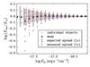 |
Fig. 4 Validation of the emission line flux integration routine utilising implanted emission lines in the MUSE HDF-S datacube described in Sect. 3.1. The input flux of the implanted emission lines is shown on the abscissa, while on the ordinate we show the logarithmic difference between input flux and measured flux by LSDCat: log Fout [ erg s-1 cm-2 ] − log Fin [ erg s-1 cm-2 ] = log (Fout/Fin). Measured fluxes are obtained in apertures of 3·RKron. Grey crosses show the obtained difference for each individual object, while the blue circle shows the mean difference of all measured fluxes at a given input flux. The red bars indicate the spread (measured standard deviation) over all measured fluxes at a given input flux, while the black bars indicate the expected spread (predicted standard deviation) according to the average uncertainty of the flux measurement at a given input flux. For clarity, the red and black bars have been offset slightly to the positive and negative, respectively, from the actual input flux. |
Given the known input emission line fluxes of the implanted fake emission line sources Fin we are equipped to validate the flux integration routine implemented in LSDCat. As detailed in Sect. 2.5.2, LSDCat integrates fluxes in circular apertures of radii k·RKron (Eqs. (26) and (27)). It has been shown that apertures with k = 3 are expected to contain >99% of the flux for Gaussian profiles (Graham & Driver 2005). Therefore we compare in this experiment Fin to the LSDCat measured flux in three Kron-radii: Fout = F(3·RKron). In absence of noise we thus expect that for every source Fout = Fin.
The result of the above comparison from our source insertion and recovery experiment is visualised in Fig. 4 where we plot, as a function of input flux, the difference between input and output flux for each individual emission line source detected by LSDCat. In addition to the individual differences we also show, again as a function of input flux, the mean and the standard deviation of the difference over all recovered sources (blue circles and red bars in Fig. 4). We can compare the latter with the expected spread in flux measurements. This expected spread is simply given by the average uncertainty on the flux measurement as tabulated by LSDCat for each input flux bin. As noted in Sect. 2.5.2, the flux measurement uncertainties follow from direct propagation of the voxel variances through Eq. (27).
As can be seen from Fig. 5, there is no bias in the recovered flux levels above input fluxes of log Fin [ erg s-1 cm-2 ] = − 17.5. Even for lower flux levels, the systematic errors are small, with (on average) 90% of the total flux being recovered. Still, at the lowest flux levels, where the detection completeness is also below 100%, a handful of implanted emission line sources are recovered with fluxes that are only ~50% (log (Fout/Fin) ≲ − 0.3) of the input flux. We checked that the larger deviations for some of the faintest simulated sources are all due to imperfections in the HDFS datacube. This experiment thus demonstrates at the same time the robustness of the flux measurement procedure in LSDCat, but also the need to use real data in quantifying the true performance of a certain measurement approach.
3.4. Comparison to manual flux integration on spatially extended objects
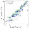 |
Fig. 5 Comparison of automatic flux measurements by LSDCat (FKron) with fluxes measured manually by curve-of-growth (FCOG) integration, for a sample of 60 Lyman α emission lines in MUSE datacubes. The automatic measurements were extracted according to Eq. (26) and Eq. (27), using spatial apertures of 2RKron (blue symbols) and 3RKron (green symbols) and adopting S / Nana = 3.5. The manual method used to measure the fluxes is explained in Sect. 3.4. The black diagonal line indicates the 1:1 relation. The gross deviation for the brightest object in the sample is caused by a strongly double-peaked Lyman α line profile with significant peak separation. Here the narrow-band window automatically determined by LSDCat treated the stronger peak as a single emission line, while the trained eye was able to adjust the window accordingly to include both peaks. |
To further demonstrate the robustness of the fluxes obtained with LSDCat, we compare the flux measurements from LSDCat with manually measured fluxes (Fig. 5). The sample on which we performed the test consists of 60 Lyman α emitting galaxies that were found by us in MUSE datacubes (Herenz et al., in prep.). As established recently by Wisotzki et al. (2016), such galaxies show regularly extended but low-surface-brightness Lyman α haloes, thus constituting good test cases for the flux measurement in non-trivially shaped extended objects. We obtained the manual flux measurements by using a curve-of-growth approach on pseudo-narrowband image created from the datacube. The width and central wavelength of those images were determined by eye in order to ensure that the complete emission line signal is encompassed within the band-pass. Therefore we utilised 1D spectra extracted in a circular aperture of three pixel radius centred on  ,
,  . On these images we then constructed the growth curve by integrating the fluxes in concentric circular apertures with consecutively increasing radii. Finally, we visually inspected these curves to pin down the radius at which the curve saturates, and the total flux within this circular aperture was adopted as the final flux measurement.
The LSDCat measurements were obtained in apertures of R = 2RKron and R = 3RKron and applying Eq. (27). As can be seen in Fig. 5, the different measurement approaches agree very well globally. The LSDCat R = 2RKron fluxes are systematically somewhat below the growth curve measurements, indicating that the 2RKron apertures still lose a small but significant fraction of the flux (–2% or –6% flux lost compared to the manual fluxes in the median or average of the sample, respectively); this is no longer the case for the R = 3RKron apertures (+10 % or +8 % flux gained in the median or average, respectively). We conclude that LSDCat delivers reliable and robust flux measurements for emission lines with non-pathological spatial and spectral shapes.
4. Guidelines for the usage of LSDCat
We now provide some guidelines for using LSDCat on wide-field IFS datacubes. These are based on our experience with applying the code on MUSE datacubes, searching for faint emission lines from high-redshift galaxies (first results presented in Bacon et al. 2015; and Bina et al. 2016; more will be reported in Herenz et al. 2017). We intend these guidelines to be instructive for the potential LSDCat user, but they should not be understood as recipes.
4.1. Dealing with bright continuum sources in the datacube
Even in relatively empty regions in the sky, any blank-field exposure will contain objects that produce a detectable continuum signal within the datacube, and that correspondingly appear in a white-light image resulting from averaging over all layers in the datacube (e.g. Fig. 3 in Bacon et al. 2015). To detect such sources, conventional 2D source detection algorithms are clearly sufficient. Since in the detection process of LSDCat we implicitly assume any significant signal to be due to emission lines, it is advisable to either mask out or, better, subtract any significant continuum signal from the datacube before running LSDCat. This step is not strictly needed, and the presence of continuum sources in the datacube does not render the detection algorithm unusable as such. But the significance of a line detection would clearly change if the line sat on top of a continuum signal, while a very bright continuum-only object would even turn out a band of spurious detections.
To remove the continuum, we found it useful to create and subtract a “continuum-only” cube by median filtering the original flux datacube in spectral direction only. The width of the median filter should be much broader than the expected widths of the emission lines, and it should be narrow enough to approximately trace a slowly varying continuum. In our experience, filter radii of ~ 150 Å–200 Å serve these goals very well. The median filter-subtracted datacube can then be used as input F for LSDCat.
4.2. Width of the spatial filter template
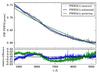 |
Fig. 6 Wavelength dependence of the PSF FWHM in the MUSE HDFS datacube (Bacon et al. 2015). The grey curve shows the FWHM from a Moffat fit to the brightest star in the field, the blue curve shows a quadratic polynomial fit to the grey curve, and the green curve shows the analytic prediction for FWHM(λ) from Tokovinin (2002; see Sect. 4.2 for details). In the bottom panel we show the relative difference between polynomial and analytic prediction from the measured PSF FWHM. The black curve in the bottom panel shows the relative difference between the analytic prediction and a polynomial fit to this prediction. |
The matched filtering approach produces maximum significance if the shapes of the true signal and of the template exactly agree; any template mismatch leads to a reduced S / Npeak value. Fortunately, this dependence of S / N on the template shape parameters is relatively weak around the optimum. If both signal and template are of Gaussian shape and the template has an incorrect width of FWHMtempl = κ × FWHMtrue, it can be shown that S/Npeak decreases only as 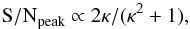 (36)(Zackay & Ofek 2017). Hence even a difference of 20% between the adopted and the correct FWHM will result in a reduction of S/N by only ~2%, entirely negligible for our purposes; this number is supported by our own numerical experiments.
When searching for compact emission line objects, a single spatial template modelling the light distribution of a point source (i.e. the PSF) will therefore be sufficient for many applications. Even neglecting the wavelength dependence of the seeing (i.e. setting the polynomial coefficient p0 in Eq. (15) to the mean Gaussian seeing FWHM, and all other PSF parameters to zero) will result in only a very modest reduction of sensitivity at the lowest and highest wavelengths.
To go one step further in accuracy, one has to account for the seeing as a function of wavelength. In the framework of the standard (Kolmogorov) turbulence model of the atmosphere, the seeing is expected to decrease with increasing wavelength as FWHM ∝ λ− 1 / 5, where the constant of proportionality also depends on airmass (e.g. Hickson 2014). In reality, other effects also play a role, such as guiding errors, or the blurring induced by co-adding multiple dithered exposures of the same field.
When the observed field contains a point source of sufficient brightness, a direct measurement of FWHM(λ) is possible from the datacube. As an example, we show in Fig. 6 the derived FWHM(λ) relation from a Moffat fit to the brightest star in the MUSE HDFS datacube (same data as Fig. 2 in Bacon et al. 2015). Here we overplot the polynomial fit according to Eq. (15) and the relative difference between this fit and the FWHM values derived from the star, (FWHMstar − FWHMfit) /FWHMstar. This difference is less than 3%, thus totally negligible in our matched-filter application. For datacubes containing only faint stars, it may be advisable to bin over several spectral layers before modelling the PSF.
If no point source is present within the datacube, the relations by Tokovinin (2002) can be used to get an idea of the dependence of FWHM on λ. They predict FWHM(λ) given a differential image motion monitor (DIMM) seeing FWHM measurement, the airmass of the observation, and an additional parameter L0 (called the wavefront outer scale length) that quantifies the maximum size of wavefront perturbations by the atmosphere (e.g. Martin et al. 1998). In Fig. 6 we also compare the FWHM(λ) relation derived from this model to the actual measurement of the brightest star in the HDFS. For the plot, we adopted a DIMM seeing of 0.75′′ at 5000 Å and an airmass of 1.41, both averages over all individual MUSE HDFS observations. We set L0 to 22 m, which is the median of this for the Paranal observatory (Conan et al. 2000). As can be seen, this model provides a very good description of the measured FWHM(λ) relation. Moreover, from this figure it is also clear that a second-order polynomial is a nearly perfect representation of the TokovininFWHM(λ) prediction.
4.3. Width of the spectral filter template
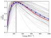 |
Fig. 7 Ratio ξ = (S / N) / (S / Nmax) for all Lyman α-emitting sources in the Hubble Deep Field South MUSE datacube from Bacon et al. (2015). Here, S/Nmax is the maximum S/Npeak value of a source, over all considered filter widths. The grey lines denote the ξ for the individual emitters, while the blue points and connecting dashed curve show the average relation. For a filter width of FWHMv = 250 km s-1 (vertical dashed line), almost all Lyman α line emitters have ξ> 90%. The red curve shows the theoretically expected ratio |

As explained above, LSDCat assumes the spectral (Gaussian) template to have a fixed width in velocity space. We now briefly demonstrate the effect of template mismatch in the spectral domain. Similarly to the 2D case considered in the previous subsection (Eq. (36)), it can be shown that S / Npeak decreases as  (37)where κ is the ratio between adopted and true template width. Even when the filter width is half or twice that of the actual object, the maximum reachable detection significance reduces by only ~ 10%. For the same reason, the achievable S / N is very robust against moderate shape mismatches between real emission line profiles and the Gaussian template profile.
A good choice of the spectral filter width FWHMv can be motivated by analysing the distribution of expected emission line widths (taking instrumental line broadening into account). If the distribution of observed line widths is relatively narrow it will be sufficient to adopt a single template with width close to the midpoint of the expected distribution. If however the expected distribution is very broad, for example, when searching both for star-forming galaxies and for AGN, it may be useful to generate two filtered datacubes with significantly different FWHM values (the ratio should be at least a factor 3). This implies two LSDCat runs creating two catalogues that later have to be merged.
To demonstrate the impact of varying the template width FWHMv on the detectability of a particular class of emission-line objects we show in Fig. 7 the dependence of the ratio ξ ≡ (S / N) / (S / Nmax) for all Lyman α emitters in the MUSE Hubble Deep Field South datacube (Bacon et al. 2015). Here, S / Nmax denotes the maximum detection significance for a line, comparing all considered line widths. The plot shows that ξ varies quite slowly with template width, confirming the theoretically expected behaviour (shown by the red curve). A good choice, at least for this object class, appears to be a filter width of FWHM = 250 km s-1, for which basically all the Lyman α emitters in the sample are detected with at least 90% of their maximum possible detection significance. The same template will capture even completely unresolved emission (i.e. with just the MUSE instrumental line width FWHM of ~100 km s-1 at λ = 7000 Å) at more than 80% of the value for a perfectly matching template.
4.4. Empirical noise calibration
Source detection is essentially a decision process based on a test statistic to either reject or accept features in the data as genuine astronomical source signals (e.g. Schwartz & Shaw 1975; Wall 1979; Hong et al. 2014; Zackay & Ofek 2017; Vio & Andreani 2016). This decision is usually based on a comparison with the noise statistics of the dataset under scrutiny. Consequently a good knowledge of the noise properties is required for deciding on meaningful thresholds, for example, in terms of false-alarm probability. In LSDCat we assume that σ2 contains a good estimate of the variances. However, in reality this is often not so easy to obtain. In particular, resampling processes carried during the data reduction usually neglect the covariance terms; even if known, it would be computationally prohibitive to formally include them in a dataset of 4 × 10⁸ voxels. In consequence, any direct noise property derived from σ2 will underestimate the true noise, possibly by a very substantial factor, and the resulting detection significances will be biased towards overly high values that lose their probabilistic connotation.
A possibly remedy is self-calibration of the noise from the flux datacube. There are several ways to accomplish this, and here we simply provide a few insights from our own experience with MUSE cubes. It must be realised that the pixel-to-pixel noise in any given spectral layer will be as much affected by the resampling as the propagated variances, and therefore biased low in the same way. This is not so, however, for the variance of a typical aperture, for which the effects of resampling are much lower (basically acting only on the pixels at the circumference of the aperture). One can therefore estimate effective variances by evaluating the standard deviation between several identical apertures placed in different blank sky locations, separately for each spectral layer. This approach also implicitly accounts for additional noise-like effects due to imperfect flatfielding or sky subtraction.
Indeed, sky subtraction residuals can still be an issue in MUSE data, especially for the OH forest in the red part of the spectral range. If a dataset should be heavily affected and suffer from too many spurious detections that are just sky residuals (and even the new ZAP software by Soto et al. 2016, not providing sufficient improvement), it is still possible to increase the effective variances for the affected spectral layers to a level where only extremely bright sources at these wavelengths are detected by LSDCat.
4.5. Choosing the detection and analysis thresholds
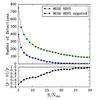 |
Fig. 8 Top panel: number of LSDCat emission line detections at different S / Ndet thresholds in the MUSE HDFS datacube (green symbols) and in a negated version of it (blue symbols). Bottom panel: expected rate of genuine detections approximated by the ratio R = (p − n) /p, where p is the number of emission line detections in the MUSE HDFS datacube and n is this number in the negated dataset. |
A crucial quantity in each detection process is the incidence rate of false positives. If the noise properties are accurately known, the false-alarm probability can be directly calculated from the detection threshold S / Ndet. Given the ≳108 voxels in a MUSE-like wide-field datacube it is obviously necessary to have a very low false-alarm probability. After matched filtering with a typical template the number of independent voxels gets reduced by a factor of ~ 102. (Here we consider as a typical template vFWHM = 300 km s-1 and p0 = 0.8″ (the default values in LSDCat). Given the spatial sampling of 0.2′′ per spatial pixel and spectral sampling of 1.25 Å per datacube layer in MUSE, this corresponds at the central wavelength range of MUSE (~6980 Å) to a filter FWHM of ~10 voxels.) Even assuming perfect Gaussian noise, a threshold of S / Ndet = 5 would then already result in ~ 10 spurious detections per cube. However, the wings of the noise distribution are never perfectly Gaussian, to which also flatfielding and sky subtraction residuals have to be added; any such deviations from Gaussianity will directly inflate the false detection rate.
Instead of relying on theoretically expected false alarm probabilities, we recommend self-calibrating the rate of spurious detections using LSDCat on the negated cube − F. While obviously no real emission line object can be detected in such a dataset, it can probably be assumed that the effective noise properties are approximately the same in original and negated data. Running LSDCat on both versions then immediately allows us to estimate the ratio of real to spurious detections and adjust the final value of S / Ndet accordingly. A possible criterion could then be the point of diminishing returns, where lowering the detection threshold would produce a large increase in spurious detections with only a small compensatory increase of genuine emission lines.
In Fig. 8 we exemplarily present the result of such an analysis for the MUSE HDFS dataset. This datacube was processed according to the guidelines given in the previous subsections. In the figure, we show both the number of detections in the original- and in the negated datacube at different thresholds. Moreover, in the bottom panel of Fig. 8 we show the ratio R = (p − n) /p, where p and n designate the number of detections in the original and negated datacube, respectively. Assuming a symmetric noise distribution around zero and no systematic negative holes in the data, the rate of genuine detections within a catalogue at a given threshold can be approximated by R (e.g. Serra et al. 2012). However, we find that the sky-subtraction residuals in the MUSE HDFS datacube appear to be systematically skewed to more negative values. In addition, since we subtracted continuum signal utilising the median filter approach (Sect. 4.1), absorption lines in some continuum bright objects created holes that mimic emission line signals in the negated datacube. Indeed, most of the detections in the negated cube at S / Ndet ≳ 10 can be associated either with sky subtraction residuals or holes from over-subtracted absorption lines. Taking this into account, we notice in Fig. 8 a second strong increase of detections in the negated dataset that is not compensated by positive detections at S / Ndet ≲ 8. Hence, for this particular dataset a threshold below S / Ndet ≈ 8 would not be advisable.
The choice of the analysis threshold S / Nana used in the measurement routine (Sect. 2.5) again depends on the noise characteristics. Here it is useful to visually inspect the S / N-cubes. Considering for example the faint emission line source presented in Fig. 2, by comparing the left panel (where no source is present) to the right panel that includes the source, we find that non-source voxels rarely obtain S / N values high than 3. Hence, in this dataset, voxels around a real detection above a threshold value of 3.5 are likely linked to the actual source and should be included in the measurement process.
5. Conclusion and outlook
Here we presented LSDCat, a conceptually simple but robust and efficient detection package for emission line objects in wide-field IFS datacubes. The detection utilises a 3D matched-filtering approach to detect individual emission lines and sorts them into discrete objects. Furthermore, the software measures fluxes and the spatial extents of detected lines. LSDCat is implemented in Python, with a focus on fast processing of the large data volumes generated by instruments such as MUSE. In this paper we also provided some instructive guidelines for the prospective usage of LSDCat.
LSDCat is open-source. Following the example of AstroPy (Astropy Collaboration et al. 2013), we release it to the community under a 3-clause BSD style license8. This license permits usage and modification of the code as long as notice on the copyright holders (E.C. Herenz & L. Wisotzki) is given. A link to download the software is provided on the MUSE Science Web Service9, and it is also available via the Astrophysics Source Code Library10 (Herenz & Wistozki 2016).
LSDCat is documented in two ways. First, each of the routines described in Sect. 2 is equipped with an online help. Secondly we provide an extensive README file describing all the routines and options in detail. Moreover, that README contains examples and scripts that help use LSDCat efficiently.
LSDCat is actively maintained as it is currently used by the MUSE consortium to search for high-z faint emission line galaxies (e.g., Bacon et al. 2015; Bina et al. 2016; Herenz et al., in prep.; Urrutia et al., in prep.). Development takes place within a git repository11. Technically inclined members of the community are invited to contribute to the code. We also offer a bug tracker that allows users to report problems with the software.
While LSDCat is fully operational, we see a number of aspects where there is room for future improvement. For example, LSDCat currently does not perform a deblending of over-merged detections, nor does it automatically merge detections belonging to a single source unless their initial positions are within a predefined radius. Indeed, in our search for faint line emitters in MUSE datacubes we encountered a few cases of very extended line-emitting galaxies that fragmented into several “sources”. We aim at addressing this problem in a future version. Currently these sources have to be merged or deblended manually in the resulting output catalogue. Another improvement planned for a future release is an automatic object classification for objects where multiple lines are detected. To this aim, the combination of spectral lines found at the same position on the sky must match a known combination of redshifted galaxy emission line peaks (Garilli et al. 2010). Finally, while in principle the software could be used for any sort of astronomical datacubes (e.g. coming from radio observations, or other IFS instruments), we have so far focused our efforts in development and testing on MUSE datacubes. However, the code is independent of instrument specifications and requires only valid FITS files following the conventions stated in Sect. 2.1. Still, despite all these possible enhancements LSDCat is already a complete software package, and we hope that it will be of value to the community.
Python Software Foundation. Python Language Reference, version 2.7. Available at http://www.python.org
NumPy version 1.10.1. Available at http://www.numpy.org/
SciPy version 0.16.1, available at http://scipy.org/
AstroPy version 1.0.1, available at http://www.astropy.org/
In the limiting case β → ∞ Eq. (12) is equal to Eq. (11); cf. Trujillo et al. (2001b).
MUSE HDFS version 1.24, available for download from http://muse-vlt.eu/science/hdfs-v1-0/
In order to follow the example we provide a suitable mask for the HDFS datacube version 1.34 in the examples folder of the LSDCat repository.
Acknowledgments
We thank Maria Werhahn for valuable help with the parameter study shown in Fig. 7 and Joseph Caruana for providing us with curve-of-growth flux integrations of 60 Lyα emitters shown in Fig. 5. We thank Rikke Saust for preparing the test data. We also thank the MUSE consortium lead by Roland Bacon for constructive feedback during the LSDCat development. E.C.H. dedicates this paper to Anna’s cute fat cat Cosmos.
References
- Akhlaghi, M., & Ichikawa, T. 2015, ApJS, 220, 1 [NASA ADS] [CrossRef] [Google Scholar]
- Allington-Smith, J. 2006, Astron. Rev., 50, 244 [NASA ADS] [CrossRef] [Google Scholar]
- Annunziatella, M., Mercurio, A., Brescia, M., Cavuoti, S., & Longo, G. 2013, PASP, 125, 68 [NASA ADS] [CrossRef] [Google Scholar]
- Astropy Collaboration,Robitaille, T. P., Tollerud, E. J., et al. 2013, A&A, 558, A33 [NASA ADS] [CrossRef] [EDP Sciences] [Google Scholar]
- Bacon, R., Vernet, J., Borisiva, E., et al. 2014, The Messenger, 157, 13 [NASA ADS] [Google Scholar]
- Bacon, R., Brinchmann, J., Richard, J., et al. 2015, A&A, 575, A75 [NASA ADS] [CrossRef] [EDP Sciences] [Google Scholar]
- Bertin, E. 2001, in Mining the Sky, eds. A. J. Banday, S. Zaroubi, & M. Bartelmann, 353 [Google Scholar]
- Bertin, E., & Arnouts, S. 1996, A&AS, 117, 393 [NASA ADS] [CrossRef] [EDP Sciences] [Google Scholar]
- Bina, D., Pelló, R., Richard, J., et al. 2016, A&A, 590, A14 [NASA ADS] [CrossRef] [EDP Sciences] [Google Scholar]
- Bourguignon, S., Mary, D., & É. Slezak 2012, Statistical Methodology, 9, 32 [CrossRef] [MathSciNet] [Google Scholar]
- Conan, R., Ziad, A., Borgnino, J., Martin, F., & Tokovinin, A. A. 2000, in Interferometry in Optical Astronomy, eds. P. Léna, & A. Quirrenbach, Proc. SPIE, 4006, 963 [Google Scholar]
- Das, P. K. 1991, Optical Signal Processing (Springer Science + Business Media) [Google Scholar]
- Filippenko, A. V. 1982, PASP, 94, 715 [NASA ADS] [CrossRef] [Google Scholar]
- Garilli, B., Fumana, M., Franzetti, P., et al. 2010, PASP, 122, 827 [NASA ADS] [CrossRef] [Google Scholar]
- Graham, A. W., & Driver, S. P. 2005, PASA, 22, 118 [NASA ADS] [CrossRef] [Google Scholar]
- Greisen, E. W., & Calabretta, M. R. 2002, A&A, 395, 1061 [NASA ADS] [CrossRef] [EDP Sciences] [Google Scholar]
- Greisen, E. W., Calabretta, M. R., Valdes, F. G., & Allen, S. L. 2006, A&A, 446, 747 [NASA ADS] [CrossRef] [EDP Sciences] [Google Scholar]
- Herenz, E. C., & Wistozki, L. 2016, LSDCat: Line Source Detection and Cataloguing Tool, Astrophysics Source Code Library [Google Scholar]
- Herenz, E. C., Urrutia, T., Wisotzki, L., et al. 2017, A&A, in press, DOI: 10.1051/0004-6361/201731055 [Google Scholar]
- Hickson, P. 2014, A&ARv, 22, 76 [NASA ADS] [CrossRef] [Google Scholar]
- Hong, S., Dey, A., & Prescott, M. K. M. 2014, PASP, 126, 1048 [NASA ADS] [CrossRef] [Google Scholar]
- Husser, T.-O., Kamann, S., Dreizler, S., et al. 2016, A&A, 588, A148 [NASA ADS] [CrossRef] [EDP Sciences] [Google Scholar]
- Jones, E., Oliphant, T., Peterson, P., et al. 2001, SciPy: Open source scientific tools for Python, [Online; accessed 2016-01-15] [Google Scholar]
- Jurek, R. 2012, PASA, 29, 251 [NASA ADS] [CrossRef] [Google Scholar]
- Kamann, S., Wisotzki, L., & Roth, M. M. 2013, A&A, 549, A71 [NASA ADS] [CrossRef] [EDP Sciences] [Google Scholar]
- Kelz, A., Kamann, S., Urrutia, T., Weilbacher, P., & Bacon, R. 2016, in Multi-Object Spectroscopy in the Next Decade: Big Questions, Large Surveys, and Wide Fields, eds. I. Skillen, M. Barcells, & S. Trager, ASP Conf. Ser., 507, 323 [Google Scholar]
- Kerutt, J. 2017, QtClassify: IFS data emission line candidates classifier, Astrophys. Source Code Library [record ascl: 1703.011] [Google Scholar]
- Koribalski, B. S. 2012, PASA, 29, 359 [NASA ADS] [CrossRef] [Google Scholar]
- Kron, R. G. 1980, ApJS, 43, 305 [NASA ADS] [CrossRef] [Google Scholar]
- Martin, C., Moore, A., Morrissey, P., et al. 2010, in SPIE Conf. Ser., 7735 [Google Scholar]
- Martin, F., Tokovinin, A., Ziad, A., et al. 1998, A&A, 336, L49 [NASA ADS] [Google Scholar]
- Masias, M., Freixenet, J., Lladó, X., & Peracaula, M. 2012, MNRAS, 422, 1674 [NASA ADS] [CrossRef] [Google Scholar]
- Meillier, C., Chatelain, F., Michel, O., et al. 2016, A&A, 588, A140 [NASA ADS] [CrossRef] [EDP Sciences] [Google Scholar]
- Moffat, A. F. J. 1969, A&A, 3, 455 [NASA ADS] [Google Scholar]
- Pence, W. D., Chiappetti, L., Page, C. G., Shaw, R. A., & Stobie, E. 2010, A&A, 524, A42 [NASA ADS] [CrossRef] [EDP Sciences] [Google Scholar]
- Popping, A., Jurek, R., Westmeier, T., et al. 2012, PASA, 29, 318 [NASA ADS] [CrossRef] [Google Scholar]
- Press, W. H., Teukolsky, S. A., Vetterling, W. T., & Flannery, B. P. 1992, Numerical recipes in FORTRAN. The art of scientific computing [Google Scholar]
- Roth, M. M. 2006, Astron. Rev., 49, 573 [NASA ADS] [CrossRef] [Google Scholar]
- Saintonge, A. 2007, AJ, 133, 2087 [NASA ADS] [CrossRef] [Google Scholar]
- Schwartz, M., & Shaw, L. 1975, Signal processing: discrete spectral analysis, detection, and estimation (Tokyo: McGraw-Hill Kogakusha, Ltd.) [Google Scholar]
- Serra, P., Jurek, R., & Flöer, L. 2012, PASA, 29, 296 [NASA ADS] [CrossRef] [Google Scholar]
- Serra, P., Westmeier, T., Giese, N., et al. 2015, MNRAS, 448, 1922 [NASA ADS] [CrossRef] [Google Scholar]
- Shore, S. N. 2009, A&A, 500, 491 [NASA ADS] [CrossRef] [EDP Sciences] [Google Scholar]
- Soto, K. T., Lilly, S. J., Bacon, R., Richard, J., & Conseil, S. 2016, MNRAS, 458, 3210 [NASA ADS] [CrossRef] [Google Scholar]
- Streicher, O., Weilbacher, P. M., Bacon, R., & Jarno, A. 2011, in Astronomical Data Analysis Software and Systems XX, eds. I. N. Evans, A. Accomazzi, D. J. Mink, & A. H. Rots, ASP Conf. Ser., 442, 257 [Google Scholar]
- Tokovinin, A. 2002, PASP, 114, 1156 [NASA ADS] [CrossRef] [Google Scholar]
- Trujillo, I., Aguerri, J. A. L., Cepa, J., & Gutiérrez, C. M. 2001a, MNRAS, 321, 269 [NASA ADS] [CrossRef] [Google Scholar]
- Trujillo, I., Aguerri, J. A. L., Cepa, J., & Gutiérrez, C. M. 2001b, MNRAS, 328, 977 [NASA ADS] [CrossRef] [Google Scholar]
- Turner, J. E. 2010, Canary Islands Winter School of Astrophysics, Vol. XVII, 3D Spectroscopy in Astronomy, eds. E. Mediavilla, S. Arribas, M. Roth, J. Cepa-Nogue, & F. Sanchez (Cambridge University Press), 87 [Google Scholar]
- van der Walt, S., Colbert, S. C., & Varoquaux, G. 2011, Comput. Sci. Eng., 13, 22 [CrossRef] [Google Scholar]
- Vio, R., & Andreani, P. 2016, A&A, 589, A20 [NASA ADS] [CrossRef] [EDP Sciences] [Google Scholar]
- Wall, J. V. 1979, Quant. J. Roy. Astron. Soc., 20, 138 [NASA ADS] [Google Scholar]
- Weilbacher, P. M., Streicher, O., Urrutia, T., et al. 2012, in SPIE Conf. Ser., 8451, 84510B [Google Scholar]
- Weilbacher, P. M., Streicher, O., Urrutia, T., et al. 2014, in Astronomical Data Analysis Software and Systems XXIII, eds. N. Manset & P. Forshay, ASP Conf. Ser., 485, 451 [Google Scholar]
- Whiting, M. T. 2012, MNRAS, 421, 3242 [NASA ADS] [CrossRef] [Google Scholar]
- Wisotzki, L., Bacon, R., Blaizot, J., et al. 2016, A&A, 587, A98 [NASA ADS] [CrossRef] [EDP Sciences] [Google Scholar]
- Zackay, B., & Ofek, E. O. 2017, ApJ, 836, 187 [NASA ADS] [CrossRef] [Google Scholar]
Appendix A: Usage example
We provide a short example to demonstrate how the user interacts with the LSDCat routines to obtain an emission line catalogue from an IFS datacube (see also Fig. 1). For this example we use the MUSE HDFS datacube (Bacon et al. 2015) in version 1.34. This datacube can be downloaded from the MUSE consortium data release web page12. For brevity, we refer to the MUSE HDFS datacube FITS file as datacube.fits. Moreover, in all following commands, the -o option specifies the output filename of a particular routine.
As detailed in Sect. 4.1 any detectable source continua should be removed from a datacube on which LSDCat is used. There we outlined, that it is often sufficient to subtract these continua by subtracting an in-spectral-direction median filtered version of the datacube from the original datacube. We package with LSDCat an additional routine median-filter-cube.py that performs this task via the following command:
median-filter-cube.py datacube.fits \ -o mf_datacube.fits(Run with its default settings the full width of the running median is 180 Å.) The output file mf_datacube.fits contains suitable input datacubes F and σ2 for the matched-filtering procedure (Sect. 2.2).
The spatial convolution and corresponding error propagation can now be achieved by running the following command:
lsd_cc_spatial.py --gaussian \ -p0=0.65 -p1=-4.5e-5 --lambda0=7050 \ -i mf_datacube.fits -m mask.fits \ -o spac_datacube.fitsHere we specified with -p0, -p1 and --lambda0 the coefficients and zero-point of the linear function p(λ [ Å ] ) = 0.65 − 4.5 × 10⁻⁵(λ [ Å ] − 7050Å) which is an apt representation of the PSF FWHM wavelength dependency in this field. The switch --gaussian models the PSF as a circular Gaussian (Eq. (11)). Here we also utilise a mask mask.fits that masks out imperfections in the HDFS datacube near the FoV borders and the brightest star in the field, as these features cause numerous unwanted detections in the datacube13. In the LSDCat documentation, we detail how such a mask can be created. The output file is named spac_datacube.fits.
Next, the spectral convolution is run on spac_datacube.fits via
lsd_cc_spectral.py -i spac_datacube.fits \ --FWHM=300 -o 3d_filtered_datacube.fitsHere --FWHM is used to specify a filter FWHM of 300 km s-1. The output 3d_filtered_datacube.fits now contains the matched filter output and from which we can compute the signal-to-noise cube S/N (Eq. (10)) via:
s2n-cube.py -i 3d_filtered_datacube.fits \ -o sncube.fitsWhile optional, the above step reduces the execution time of the routines lsd_cat.py and lsd_cat_measure.py, as they normally would create the S/N datacube on the fly.
We can now create an emission line source catalogue with S / Ndet> 10 by typing:
lsd_cat.py -i sncube.fits -t 10 -c catalogue.cat.Utilising the thresholding procedure described in Sect. 2.4, the above command creates a ASCII and FITS table catalogue.cat and catalogue.fits for 2456 emission line candidates from 225 potential individual objects. Finally, the basic measurements described in Sect. 2.5 are obtained for each of the emission line candidates with the command
lsd_cat_measure.py -ic catalogue.fits -ta 5 \ -f mf_datacube.fits \ -ff 3d_filtered_datacube.fits \ -ffsn sncube.fits.At this stage we recommend the catalogue to be inspected with QtClassify14, a graphical user interface that helps to classify emission line candidates in IFS data, and which is optimally suited to work with catalogues created by LSDCat (Kerutt 2017).
More complete and up-to-date documentation describing all the routines can be found in the LSDCat repository. Moreover, for all routines, on-line usage information can be displayed by calling them with the -h switch.
All Tables
All Figures
|
Fig. 1 Flowchart illustrating the processing steps of LSDCat from an input datacube to a catalogue of positions, shape parameters, and fluxes of emission line sources. |
| In the text | |
|
Fig. 2 Example of the effect of matched filtering on the detectability of a faint emission-line source in the MUSE datacube of the Hubble Deep Field South (Bacon et al. 2015). Shown is a Lyman α emitting galaxy at redshift z = 3.278 with flux FLyα = 1.3 × 10⁻¹⁸ erg s-1 (ID #162 in Bacon et al. 2015). The panels in the first row display four different spectral layers of the continuum-subtracted datacube F. The second row shows the same spectral layers, but for the filtered S / N cube (Eq. (9)) that was used to build the catalogue of emission line sources via thresholding (Eq. (18)). The leftmost panels show a layer significantly away from the emission line peak, the other panels show layers at spectral coordinates zpeak − 1, zpeak, and zpeak + 1, respectively, where zpeak designates the layer containing the maximum S / N value of the source. The third row shows the flux density spectrum in the spaxels at (xpeak,ypeak) and (xpeak ± 1,ypeak ± 1), where xpeak and ypeak are the spatial coordinates of the highest S/N value. The bottom row shows a S/N spectrum extracted from the S / N cube at xpeak and ypeak. |
| In the text | |
|
Fig. 3 Completeness curve |
| In the text | |
|
Fig. 4 Validation of the emission line flux integration routine utilising implanted emission lines in the MUSE HDF-S datacube described in Sect. 3.1. The input flux of the implanted emission lines is shown on the abscissa, while on the ordinate we show the logarithmic difference between input flux and measured flux by LSDCat: log Fout [ erg s-1 cm-2 ] − log Fin [ erg s-1 cm-2 ] = log (Fout/Fin). Measured fluxes are obtained in apertures of 3·RKron. Grey crosses show the obtained difference for each individual object, while the blue circle shows the mean difference of all measured fluxes at a given input flux. The red bars indicate the spread (measured standard deviation) over all measured fluxes at a given input flux, while the black bars indicate the expected spread (predicted standard deviation) according to the average uncertainty of the flux measurement at a given input flux. For clarity, the red and black bars have been offset slightly to the positive and negative, respectively, from the actual input flux. |
| In the text | |
|
Fig. 5 Comparison of automatic flux measurements by LSDCat (FKron) with fluxes measured manually by curve-of-growth (FCOG) integration, for a sample of 60 Lyman α emission lines in MUSE datacubes. The automatic measurements were extracted according to Eq. (26) and Eq. (27), using spatial apertures of 2RKron (blue symbols) and 3RKron (green symbols) and adopting S / Nana = 3.5. The manual method used to measure the fluxes is explained in Sect. 3.4. The black diagonal line indicates the 1:1 relation. The gross deviation for the brightest object in the sample is caused by a strongly double-peaked Lyman α line profile with significant peak separation. Here the narrow-band window automatically determined by LSDCat treated the stronger peak as a single emission line, while the trained eye was able to adjust the window accordingly to include both peaks. |
| In the text | |
|
Fig. 6 Wavelength dependence of the PSF FWHM in the MUSE HDFS datacube (Bacon et al. 2015). The grey curve shows the FWHM from a Moffat fit to the brightest star in the field, the blue curve shows a quadratic polynomial fit to the grey curve, and the green curve shows the analytic prediction for FWHM(λ) from Tokovinin (2002; see Sect. 4.2 for details). In the bottom panel we show the relative difference between polynomial and analytic prediction from the measured PSF FWHM. The black curve in the bottom panel shows the relative difference between the analytic prediction and a polynomial fit to this prediction. |
| In the text | |
|
Fig. 7 Ratio ξ = (S / N) / (S / Nmax) for all Lyman α-emitting sources in the Hubble Deep Field South MUSE datacube from Bacon et al. (2015). Here, S/Nmax is the maximum S/Npeak value of a source, over all considered filter widths. The grey lines denote the ξ for the individual emitters, while the blue points and connecting dashed curve show the average relation. For a filter width of FWHMv = 250 km s-1 (vertical dashed line), almost all Lyman α line emitters have ξ> 90%. The red curve shows the theoretically expected ratio |
| In the text | |
|
Fig. 8 Top panel: number of LSDCat emission line detections at different S / Ndet thresholds in the MUSE HDFS datacube (green symbols) and in a negated version of it (blue symbols). Bottom panel: expected rate of genuine detections approximated by the ratio R = (p − n) /p, where p is the number of emission line detections in the MUSE HDFS datacube and n is this number in the negated dataset. |
| In the text | |
Current usage metrics show cumulative count of Article Views (full-text article views including HTML views, PDF and ePub downloads, according to the available data) and Abstracts Views on Vision4Press platform.
Data correspond to usage on the plateform after 2015. The current usage metrics is available 48-96 hours after online publication and is updated daily on week days.
Initial download of the metrics may take a while.