| Issue |
A&A
Volume 601, May 2017
|
|
|---|---|---|
| Article Number | A131 | |
| Number of page(s) | 13 | |
| Section | Cosmology (including clusters of galaxies) | |
| DOI | https://doi.org/10.1051/0004-6361/201630200 | |
| Published online | 22 May 2017 | |
Generalised model-independent characterisation of strong gravitational lenses
I. Theoretical foundations
1 Universität Heidelberg, Zentrum für Astronomie, Institut für Theoretische Astrophysik, Philosophenweg 12, 69120 Heidelberg, Germany
e-mail: This email address is being protected from spambots. You need JavaScript enabled to view it.
2 Heidelberg Institute for Theoretical Studies, 69118 Heidelberg, Germany
Received: 6 December 2016
Accepted: 2 February 2017
Abstract
We extend our model-independent approach for characterising strong gravitational lenses to its most general form to leading order and use the orientation angles of a set of multiple images with respect to their connection line(s) in addition to the relative distances between the images, their ellipticities, and time-delays. For two symmetric images that straddle the critical curve, the orientation angle additionally allows us to determine the slope of the critical curve and a second (reduced) flexion coefficient at the critical point on the connection line between the images. It also allows us to drop the symmetry assumption that the axis of largest image extension is orthogonal to the critical curve. For three images almost forming a giant arc, the degree of assumed image symmetry is also reduced to the most general case, describing image configurations for which the source need not be placed on the symmetry axis of the two folds that unite at the cusp. For a given set of multiple images, we set limits on the applicability of our approach, show which information can be obtained in cases of merging images, and analyse the accuracy achievable due to the Taylor expansion of the lensing potential for the fold case on a galaxy cluster scale Navarro-Frenk-White-profile, a fold and cusp case on a galaxy cluster scale singular isothermal ellipse, and compare the generalised approach with our previously published one. The position of the critical points is reconstructed with less than 5′′ deviation for multiple images closer to the critical points than 30% of the (effective) Einstein radius. The slope of the critical curve at a fold and its shape in the vicinity of a cusp deviate less than 20% from the true values for distances of the images to the critical points less than 15% of the (effective) Einstein radius.
Key words: dark matter / gravitational lensing: strong / methods: data analysis / methods: analytical / galaxies: clusters: general / galaxies: luminosity function, mass function
© ESO, 2017
1. Introduction and motivation
While information from the second-order multipole moments of weakly distorted sources is routinely extracted in weak lensing, Bartelmann & Schneider (2001), Kaiser et al. (1995), Refregier & Bacon (2003), Seitz & Schneider (1995), we show that these multipole moments also yield vital information about the lensing potential when being extracted from multiple images in the strong lensing regime. We generalise the approach developed in Wagner & Bartelmann (2016) by including the orientation angle of the semi-major axis of the images into our set of observables, and thereby reconstruct the critical curve in the vicinity of multiple images for image configurations of two images that straddle the critical curve and for three images almost forming a giant arc without assuming any lens model. We aim to demonstrate that a lot of information contained in multiply-imaged source observations is still unused and can be easily employed to retrieve local, general properties of the lensing potential without the need of highly degenerate model fitting or ad hoc fine-tuning by adding substructure.
The paper is organised as follows: Sect. 2 briefly reviews the method as developed in Wagner & Bartelmann (2016) and presents the definitions of observables and assumptions required before listing the characteristics of the lensing potential that can be inferred from the observables. In Sect. 3 we analyse the influence of the Taylor expansion on the reconstruction of the critical curve and the ratios of potential derivatives and calculate which information can be retrieved in the case of overlapping images. As a simple test case, we show a simulated galaxy cluster consisting of a Navarro-Frenk-White (NFW) profile as gravitational lens and a Sérsic profile for the sources in Sect. 4. We discuss the results from the simulation and show the accuracy limits of the Taylor expansion under the influence of the finite pixel resolution and the approximation of the image shape as quadrupole moment. Subsequently, we show the reconstruction of the critical curve and the potential derivatives obtained by the generalised approach for multiple images at a fold and cusp in a simulated galaxy cluster scale singular isothermal ellipse (SIE) and compare the results to those obtained without taking into account the image orientations. Section 5 summarises the results and gives an outlook to the next steps necessary to make our approach applicable to observations.
Being the first part of a series of papers, this work introduces the general formalism and the complete set of observables for the leading order Taylor expansion. In subsequent papers, we will analyse realistic simulations like the HERA cluster, Meneghetti et al. (2017), and investigate the influence of the source properties, as well as biases and uncertainties introduced by the observation process in detail.
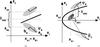 |
Fig. 1 Coordinate systems and definitions of observables for two images close to a fold critical point a) and three images close to a cusp critical point b). The thick black line in a) and parabola in b) show the approximation of the critical curve in the vicinity of the images. The fold critical point under analysis in a) is located at the crossing of the critical curve and the connection line of image A and B. The cusp critical point in b) is the vertex of the parabola. |
2. Observables and generalised approach
2.1. Definitions and assumptions
We expand the gravitational lensing potential φ(x,y) in a Taylor series around a point on the critical curve, x0 ∈ R2, and its respective point on the caustic, y0 ∈ R2, as described in detail in Wagner & Bartelmann (2016) and transform it into a coordinate system in which  (1)hold. A subscript i of φ denotes the partial derivative in xi-direction, i = 1,2, and the superscript (0) indicates that this derivative is evaluated at the singular point. We then employ as observables
-
the time delay tij = ti−tj between the arrival times of two images i and j;
-
the relative coordinate distances δij1 = xi1−xj1 and δij2 = xi2−xj2 between two images i, j along the axes of the coordinate system defined by Eq. (1);
-
the axis ratio ri = bi/ai between the semi-minor axis bi and the semi-major axis ai of the quadrupole moment of image i;
-
the orientation angle ϕi between the semi-major axis of image i and the x1-axis of the coordinate system chosen by Eq. (1)(we will also use λi ≡ cos(ϕi)/sin(ϕi));
-
the flux ratios μi/μj between image i and j, representing the magnification ratios;
-
if time delay information is available, we also require the redshift of the source, zs, and the lens, zd, to calculate the angular diameter distances between the observer and the source, Ds, between the observer and the lens, Dd, and between the lens and the source, Dds, which yield the distance factor Γd ≡ (DdDs)/(Dds)(1 + zd).
Figure 1 illustrates the definitions of observables and choices of coordinate systems for the fold configuration consisting of two images (a) and for the cusp configuration consisting of three images (b).
We assume that the images are located so close to the critical curve that intrinsic ellipticities are negligible compared to the distortions caused by lensing. This assumption is justified, as it can be shown that the observables of the images are completely dominated by the lens mapping on the critical curve and that the influence of the lens decreases for increasing distance from the critical curve (see Appendix A for details). The analysis of the intrinsic properties and higher order effects will be treated separately.
2.2. Resulting (ratios of) potential derivatives at folds
We assume that a source is close to a fold singular point of the caustic such that it is mapped to two images in the lens plane denoted by A and B. They straddle the critical curve, as shown in Fig. 1 (right). We assume, without loss of generality, that A has positive and B negative parity. As derived in more detail in Appendix B, we obtain from the observables of these two images 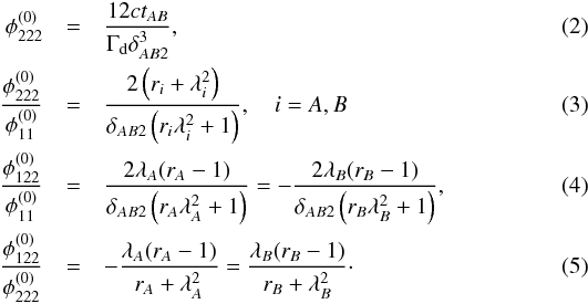 For | ϕi | = π/ 2, Eq. (3)becomes Eq. (10) of Wagner & Bartelmann (2016). If the time delay has been measured, Eqs. (3)and (4)can be solved for
  and
and  . Although Eq. (5)can be determined from Eqs. (3)and (4), we explicitly show this ratio as it is equal to the slope of the critical curve at x0. For | ϕi | = π/ 2, it becomes zero so that the images and critical curve are orthogonal to each other. Significant deviations between the ratios obtained from A and B can arise, if the images are too far from the critical curve for the assumption | μA | = | μB | to hold or if a measurement bias (e.g. due to microlensing or dust extinction) has not been taken into account yet.
The positions of A and B with respect to the critical point under consideration are given by 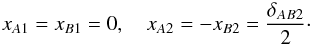 (6)
(6)
2.3. Resulting (ratios of) potential derivatives at cusps
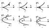 |
Fig. 2 Analysis of the observables in three images d)–f) determines whether to apply the fold or cusp equations and where the source is located with respect to the folds and cusp a)–c): a fold configuration a) and e) shows two highly symmetric images, A, B, with larger separation to the third image, C, less magnified than A, B. In a cusp configuration b) and e), c) and f), A is highly magnified compared to B and C because it can be considered an overlay of two images generated by lensing at the upper and the lower fold which unite at the cusp point. Image shapes are neglected in these graphs, but high and low absolute values of magnifications are indicated by dark and light grey values, respectively. |
The images A, B, and C close to a cusp cannot be treated equally because they have different distances to the critical point. To obtain the best Taylor approximation of the (ratios of) potential derivatives, observables from A (which is closest to the cusp, i.e. the expansion point of the Taylor series) are used in combination with those from B or C. Combinations of observables from B with C are not employed. They yield less accurate results because B and C are farther from the cusp, as is shown in Sects. 4.5.4 and 4.5.5. They are also linearly dependent on the other combinations and therefore do not contain further information. As detailed in Appendix C, we obtain for the (ratios of) potential derivatives 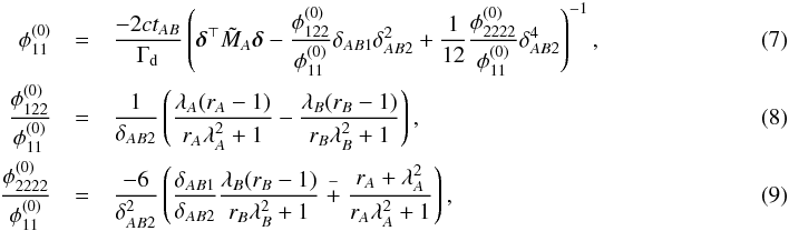 and for the position of A with respect to x0 = (0,0)
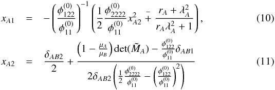 with
with 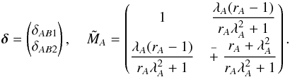 (12)The upper signs indicate a positive cusp configuration with positive
  and A having negative parity. The lower signs are valid for a negative cusp configuration with negative and a positive parity A (see Petters et al. 2001).
The slope mc of the parabola that approximates the critical curve in the vicinity of the images and has its vertex in x0 = (0,0) is then given by 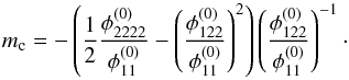 (13)Given time delay information, the cusp type can be determined. Fixing the sign of the x1-coordinates of A, B, and C, all signs of the potential derivatives are also fixed.
Replacing the observables from B by those from C, we determine the ratios of potential derivatives from the combination of A and C. For each combination of images, A and B and A and C, we thus obtain (ratios of) potential derivatives and a parabolic approximation of the critical curve in the vicinity of all three images. If the results using the pair (A, B) and using the pair (A, C) in Eqs. (7)–(13)coincide within the measurement uncertainty and the bias due to the Taylor expansion, the two folds that unite to the cusp point are symmetric. Any significant deviation between the results can be caused by an as yet unaccounted for measurement bias in an observable or an asymmetry in the mass density causing this cusp in the lens map, so that the Taylor approximation becomes inapplicable.
3. Accuracy and limits
3.1. Biases due to Taylor expansions
In general, as already stated in Wagner & Bartelmann (2016), the accuracy of the approach depends on the terms of the Taylor expansion of the lensing potential that are taken into account. In this leading order approach, we neglect  when establishing the lensing equations for the fold and assume that
  . For the cusp, we omit
  and the fourth-order derivatives except
  . Furthermore, we neglect the flexion coefficient at the location of the image, assuming that it is much smaller than the distortions caused by convergence and shear1.
Secondly, the accuracy of the results is determined by the relative distances between the images and the expansion point of the Taylor series, i.e. the critical point. As the approach also includes shape information, the quadrupole moment may be biased by higher order shape distortions.
In order to investigate the impact of these approximations and assumptions on the accuracy, simulations are set up, as detailed in Sect. 4. Furthermore, we investigate the impact of including the orientation angle compared to the approach of Wagner & Bartelmann (2016) without image orientations.
3.2. Analysis of observed triple-image configurations
To leading order Taylor expansion, the two images of a fold configuration are assumed to be so close to the critical curve that the images have a high symmetry with similiar shapes and equal absolute fluxes. Hence, finding an image configuration with observables that fulfil this criterion, we apply the equations for the fold case. In cases where a third image is close by, we can additionally apply the equations for the cusp configuration to retrieve information about the cusp critical point. Then, two approximations to the critical curve – a linear one from the fold evaluation and a parabolic one from the cusp evaluation – in the vicinity of the two images with high symmetry are obtained. In the following, we derive the relationship between them.
The (ratios of) potential derivatives obtained at the cusp point will be subject to a higher deviation due to the Taylor expansion because a “genuine” cusp configuration occurs when the source is close to both folds (and thus close to the cusp) causing the magnifications of the two outer images to become equal and about half of the magnification of the inner one. Figure 2 sketches the situations qualitatively.
We can also determine the relationship between the approximations of the critical curve of the fold and cusp configuration in the case of a triple-image configuration. As a simple example, we place a source on the y1-axis: y = (ys,0). Then, the difference in the x2-coordinate between the critical point of the parabolic approximation xc and the critical point of the linear approximation xf at the x1-value of the fold critical point between A and B is given by  (14)with
  (15)The derivation of this equation can be found in Appendix D. Figures 3a and e visualise the comparison. Equation (14)implies that the parabolic approximation of the critical curve always has a higher x2-value than the linear approximation and that the difference decreases for decreasing distance to the cusp critical point, i.e. ys → 0. The distance d of the source to the fold yf and the cusp singular point yc also determines which approximation of the critical curve is the more precise one
  As the source position is not an observable, we use the lensing equations to find the respective distances in the image plane
  An example for Eqs. (16)and (18)is given in (b) and (e) of Fig. 3 and an example for Eqs. (17)and (19)is shown in (c) and (f) of Fig. 3. Section 4.5.5 treats the case of a three-image configuration in an SIE.
3.3. Treatment of giant arc(let)s
Approaching the caustic with the source, the distortions of the images increase and their relative distances decrease. When they merge to a giant arc(let), all equations employing the observables of the individual images become inapplicable, including the time delay.
In the coordinate system defined in Eq. (1), two images enclosing a fold critical point will merge to a straight line with slope mf perpendicular to the critical curve, which we denote as arclet. Then, Eq. (5)is replaced by  (20)which is the only information we can retrieve from this degenerate fold configuration.
The three images close to a cusp will merge into a giant arc that can be approximated by the parabola with the slope given by Eq. (13). From the fitting procedure, we can also read off the vertex position, obtaining the cusp critical point.
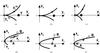 |
Fig. 3 Comparison between the approximations of the critical curve as a parabola (cusp) or a line (fold) for a given source position a) shows that the fold critical point always lies below the cusp critical point in the image plane d). Depending on the distance of the source to the caustic a)–c) and the images to the critical curve d)–f), the fold approximation is more precise than the cusp approximation b) and e) or vice versa c) and f). Image C, not being relevant for the argument, is omitted here. |
4. Simulations
In order to set confidence bounds on the quantities in Eqs. (2)−(5)and Eqs. (7)−(9), we simulate a series of gravitational lenses with decreasing degrees of symmetry: in this paper, we start with a NFW mass density profile, Navarro et al. (1996), which is usually chosen as a starting point when modelling lensing dark matter halos at galaxy cluster scale. By this simulation, we analyse the deviations due to the Taylor approximation and the fit of the quadrupole moment to the true image shape for Eqs. (2)–(5). Owing to the axisymmetry of the model, the images are orthogonal to the critical curve, so that we expect Eqs. (4)and (5)to be zero. Making the lens heavier than usual galaxy cluster scale lenses, we increase the influence of higher order potential derivatives and we investigate how well the potential derivatives of Eqs. (2)–(5)are reconstructed from the quadrupole moment of the images.
Subsequently, we simulate a galaxy cluster scale SIE, which is one of the simplest lenses in which cusps occur and in which multiple images are no longer orthogonal to the critical curve. This lens type is usually employed to model galaxy scale lenses. We use it on the galaxy cluster scale to test the validity of Eqs. (2)–(13)in the vicinity of folds and cusps where the orientation angles of the images differ from each other. In a subsequent paper, we will use the HERA cluster simulation, Meneghetti et al. (2017), as the most realistic test case on galaxy cluster scale currently available. For all multiple images in all simulations to have comparable resolution, we use a redshift of zd = 0.507 for all lenses, zs = 2 for all sources, and construct the (effective) Einstein radius at which we consider the multiple images to be about 23″.
4.1. Simulation of sources
We implement a circular Sérsic profile, Graham & Driver (2005), 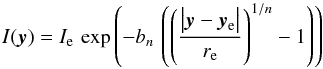 (21)in the source plane, y = (y1,y2), and normalise the intensity to 1 at the peak ye. We set n = 4, i.e. bn = 7.669, and consider a characteristic radius re = 25 px. As source redshift, we set zs = 2, so that our source model represents simplified elliptical galaxies of some ten kiloparsecs, if we set 1 px = 0.1108′′2, as in the image plane.
4.2. Simulation of the NFW lens
We simulate a NFW profile with κs = 3 and rs = 33″ for the normalising convergence and the scale radius in the notation of Bartelmann (1996). As our approach can only describe fold configurations close to radial arcs in axisymmetric models, we set the radial Einstein radius to be 23″. This implies, that we do not obtain a physically realistic galaxy-cluster-sized gravitational lens with a mass of 2.3 × 10¹⁵M⊙ inside this radius, yet, it will clearly show the influence of higher order moments on the extraction of observables and the ratios of potential derivatives.
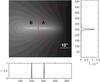 |
Fig. 4 Two-dimensional logarithmic intensity distribution of two images close to the radial critical curve, saddle point image B (left), maximum close to the lens centre A (right), critical curve (red), and centre of the lens (red cross). The plots at the right and bottom show vertical and horizontal intensity profiles through the critical point between A and B (red dot). |
We place 40 sources in steps of 1 px from each other, starting at the caustic going towards the centre of the lens, and map them to the image plane, given the lens mapping from the NFW profile. As a result, we obtain two images close to the radial critical curve as shown in Fig. 4, one saddle point image called image B, and one maximum called image A.
4.3. Simulation of the SIE lens
As a second example, we simulate an SIE with an axis ratio f = 0.6091 and a scale radius of rs = 17″, as shown in Fig. 5. To investigate the Taylor bias at a fold configuration, we choose a fold point between the images A and B (marked by the red dot in Fig. 5) and simulate eight image pairs from Sérsic sources, as described in Sect. 4.1, with increasing distance from the caustic towards the centre of the lens.
To investigate the cusp configuration of the images A, B, and C, we place Sérsic sources with increasing distance from the cusp in the caustic on the line connecting the lens centre and the cusp.
In addition, we simulate two configurations close to the cusp, one where the source is at the same y1 but y2 is once chosen to be zero, and one off the symmetry axis so that A and B approach each other to test the statements made in Sect. 3.2.
4.4. Extraction of observables
In order to determine the observables from the multiple images close to the critical curve, we employ SExtractor, Bertin & Arnouts (1996). We use the centre of light of the images as the relative distance of the images, and determine their ellipticities and orientation angles from their second-order moments. In order to calculate them SExtractor requires a segmentation into foreground objects (gravitationally lensed images) and the background. As our data is noise free, we only threshold the raw images without applying a median filter or a background subtraction. The observables determined from second-order moments depend on the threshold and we will investigate the influence of the threshold on the accuracy of the reconstruction in Sect. 4.5.2.
The observables for all images are subsequently transformed into the coordinate system defined by Eq. (1)and then inserted into Eqs. (2)–(13).
4.5. Evaluation
4.5.1. Measures for the accuracy of the approach
To estimate the accuracy of the time delay we replace  (22)in Eqs. (2)and (7)and calculate the potential difference between two images A and B from the simulated model.
As a measure for the deviation, we divide the (ratios of) potential derivatives as obtained from Eqs. (2)–(5)and Eqs. (7)–(9)by their true values given by the lens model. Analogously, we assess the deviation between Eq. (13) and the respective ratio of true ratios of potential derivatives in the cusp case. Deviations of the parabolic approximation from the critical curve are shown in the graphs in Sects. 4.5.4 and 4.5.5.
The difference between the true fold position, xt, and the reconstructed one, xr, is calculated as 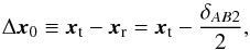 (23)using the distance between the intensity mean of A and B as δAB2. To determine the cusp critical point we employ Eqs. (10)and (11)and subtract the results from the position of image A.
4.5.2. Evaluation of NFW (fold configuration)
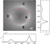 |
Fig. 5 Two-dimensional logarithmic intensity distribution of the four images generated by an SIE. The saddle point image A and the two minima B and C to the right of the lens centre (red cross) are used as cusp configuration, and A and B as configuration close to a fold (red dot). The plots at the right and bottom show vertical and horizontal intensity profiles through the critical point between A and B (red dot). |
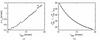 |
Fig. 6 Evaluation of the NFW profile: deviation of the reconstructed critical point from the true one, as defined in Eq. (23), dependent on the (observable) relative distance between the intensity mean of the two images a). Accuracy of Eq. (2)dependent on the same distance between images A and Bb). |
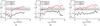 |
Fig. 7 Evaluation of the NFW profile: ratio of Eq. (3)divided by the true value for image A (black solid line) and image B (red dashed line) for a low SExtractor threshold a); an intermediate threshold b); and a high threshold c). Vertical dotted lines indicate the minimum distance at which A and B are thresholded as two separate objects. The grey-shaded area marks 10% deviation from the true ratio. |
First, we evaluate the accuracy of the reconstruction of the critical point, as shown in Fig. 6. From Fig. 6a, we read off that the reconstructed critical point is systematically shifted towards the saddle point image (as the positive x1-axis points from B to A). The deviation increases for increasing distance of the images from the critical curve, i.e. the expansion point of the Taylor series of the lensing potential. The reconstructed position of the critical point is biased towards image B because its distance to the critical point increases faster than the distance of image A to the critical point when moving the source away from the caustic.
Next, we evaluate the accuracy of Eq. (2)using Eq. (22)and plot the results in Fig. 6b. The accuracy decreases with decreasing distance from the critical curve as δAB2 in the denominator of Eq. (2)approaches zero. The steep decrease in accuracy is consistent with the results for point sources in elliptical models, as shown in Wagner & Bartelmann (2016), where we found that the deviation between  from the potential difference Δφ increases for increasingly axisymmetric lenses.
Then, we insert the observables into Eq. (3)to determine its accuracy. Figure 7 shows the results for increasing threshold 5 × 10⁴, 2 × 10⁵, 3 × 10⁵ from (a) to (c). For small relative image separations (marked by the vertical dotted lines in Fig. 7), the threshold is too low, so that SExtractor calculates the second-order moments from two merging images, which means our approach cannot be applied because of incorrectly determined observables. Between relative image separations of 10″ and 20″ lies the range of applicability of our approach. Farther away from the critical curve, the assumption | μA | = | μB | breaks down within the precision set by an HST-like gain of 2 to determine the uncertainty of the image fluxes in the SExtractor configuration file.
Comparing the results for image A and B, we find that the ratio of potential derivatives is more accurate for image B for any threshold because A is smaller and at the resolution limit to extract rA. For increasing distances from the critical curve, the images also become fainter so that the number of pixels belonging to one image, i.e. its resolution, decreases for a fixed threshold. The alternating local peaks and minima in the curves for A are effects of the pixelisation. The same effect is clearly observed for B for the highest threshold and mildly at large distances for the intermediate threshold. Focusing on B, the true ratio of potential derivatives can be reconstructed with deviations of less than 22% for all thresholds. As δAB2 is the same for all thresholds and the isocontours of the images are self-similar for fixed δAB2, the differences between the graphs in Fig. 7 show the influence of the pixelisation and resolution of r.
Owing to the unphysically high mass of the simulated NFW lens, the distorted images show features of flexion that will not be as pronounced in realistic images. Hence, retrieving the ratios of potential derivatives shown in Fig. 7 to such a high accuracy shows that possible influences of higher order shape distortions to the quadrupole moment cannot be large.
As images A and B are oriented orthogonal to the critical curve, Eq. (4)always yields zero, resulting in a slope of zero (Eq. (5)). We omit the graphs for these ratios of potential derivatives here, as the orthogonality is reproduced well because SExtractor correctly determines | ϕi | = π/ 2,i = A,B in all cases.
4.5.3. Evaluation of SIE (fold configuration)
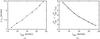 |
Fig. 8 Evaluation of the SIE profile (fold): deviation of the reconstructed critical point from the true one, as defined in Eq. (23), dependent on the (observable) relative distance between the intensity mean of the two images a). Accuracy of Eq. (2)dependent on the same distance between images A and Bb). |
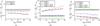 |
Fig. 9 Evaluation of the SIE profile (fold): ratio of Eq. (4)divided by the true value for image A (black solid line) and image B (red dashed line) a). Ratio of Eq. (3)for image A and B and for both images under the symmetry assumption that their orientation is orthogonal to the critical curve (blue dotted line, green dash-dotted line) b). Slope of the critical curve, Eq. (5), at the fold using the ratios obtained in a) and b) c). The grey-shaded area marks 10% deviation from the true ratio. |
Analogously, we proceed for the SIE, determine one SExtractor threshold for all simulated multiple images at increasing distance from the fold such that pixelisation effects are negligible, and extract the observables. Inserting them into Eqs. (2)–(5), we obtain the results shown in Figs. 8 and 9. Compared to the (unrealistic) NFW profile, the inaccuracy of reconstruction of the critical curve is higher by about a factor of two. The inaccuracy of  is lower by roughly a factor of ten, but is still too high to be of use to break the mass-sheet-degeneracy. Comparing this accuracy to that for and achievable close to the cusps discussed in Sect. 4.5.4, we note that the expansion of the potential to third order at folds is not a sufficient approximation and higher orders have to be included.
From Fig. 9a, we read off that the observables from the image with positive parity, B, approximate  best with deviations between 13% and 18% from the true value. (b) shows that the assumption of images orthogonally oriented to the critical curve yields accuracies of
  in the range of 90% and including information about the orientation angle yields worse results. Consequently, the accuracy of the slope of the critical curve at the fold is highest for image B using the orthogonality assumption to determine . In all three graphs, the accuracy of the reconstruction using the image orientation angles visibly decreases with increasing distance from the fold point where other critical points gain influence. Hence, the image orientation angles and their difference give hints at local asymmetries in the lens map. Using the symmetry assumption of images orientated orthogonal to the critical curve for Eq. (3), its accuracy is almost constant over the distance range, supporting this statement.
On the whole, the highest accuracy for all properties of the critical curve that can be retrieved by our approach at a fold point is obtained by using the orientation angle of the images only when calculating Eq. (4)and assuming ϕi = π/ 2, i = A,B, in Eq. (3).
4.5.4. Evaluation of SIE (symmetric cusp configuration)
Next, we investigate the accuracy of Eqs. (7)–(13)for three-image configurations generated by sources placed at increasing distance on the symmetry axis connecting the lens centre and the cusp in the caustic (see Sect. 4.3). We also compare the accuracy achievable by Eqs. (7)–(13)with the accuracy that is obtained by the approach stated in Wagner & Bartelmann (2016), which makes the symmetry assumption that the semi-major axes of all images are oriented parallel to the critical curve at the cusp. This assumption amounts to the Taylor-expanded lens mapping detailed in Petters et al. (2001) and its range of validity around the cusp point is smaller than the range of validity of the approach described in Schneider et al. (1992), on which our current approach is based.
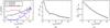 |
Fig. 10 Evaluation of the SIE profile (cusp): deviation of the reconstructed critical point from the true one dependent on the (observable) relative distance between the intensity mean of the two images A and B using the pair (A,B) (black solid line), the pair of positive parity images (B,C) (red dashed line) or the pair (A,B) with the symmetry assumption that image orientation angles are parallel to the critical curve at the cusp (blue, dash-dotted line) a). Using (A,C) yields the same result as (A,B) because the source lies on the symmetry axis between B and C. The accuracy of Eq. (7)dependent on the same distance between images A and Bb) and accuracy of the analogue to Eq. (7) under the symmetry assumption stated in Wagner & Bartelmann (2016)c). |
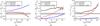 |
Fig. 11 Evaluation of the SIE-profile (cusp): ratio of Eq. (8)divided by the true value for the same configurations of image pairs and the symmetry assumption as in Fig. 10. The result for (A,B) (black solid line) coincides with the one for (B,C) (red dashed line) a). The ratio of Eq. (9)divided by the true value b). The slope of the critical curve at the cusp, Eq. (13), using the ratios obtained in a) and b) c). The grey-shaded area indicates a 10% deviation from the true ratio. |
Figure 10a shows the accuracy of the cusp point reconstruction in the image plane inferred from different combinations of image pairs. As expected, using the two positive parity images B and C to reconstruct the cusp position is the most unreliable estimate, while the approach stated in Wagner & Bartelmann (2016) using the pair (A,B) is superior to the approach including the orientation angles for the same image pair close to the critical curve. This result can also be seen in Fig. 12a comparing the position of the vertices of the parabolic approximations to the critical curve. However; as (b) shows, taking the orientation angles of the images into account yields a more accurate estimate of the cusp point when the symmetry of the image configuration is broken, i.e. for sources that do not lie on the axis connecting the lens centre and the cusp in the caustic.
As Eq. (7)diverges at the critical curve, like Eq. (2), the inaccuracy is of the same order as that of Eq. (2). Figures 10b and c shows that breaking the mass-sheet degeneracy may only be achieved to an accuracy below 10% in a small interval of relative distances between A and B under the symmetry assumption stated in Wagner & Bartelmann (2016). However, as Fig. 11 shows, the accuracies of Eqs. (8), (9), and (13)are of the order of 5% to 25%, such that the resulting potential derivatives (convergence, shear, and flexion) are still prone to high inaccuracies.
All graphs in Fig. 11 clearly show that the accuracy of the ratios of potential derivatives is vastly improved if the image orientation angles are taken into account. This can be visually confirmed in Fig. 12 by comparing the reconstruction of the critical curve according to (Wagner & Bartelmann 2016, green curve) with the reconstructions obtained from different combinations of images including their orientation angles.
4.5.5. Evaluation of SIE (asymmetric cusp configuration)
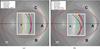 |
Fig. 12 Evaluation of the SIE profile (cusp): reconstruction of the critical curve close to a cusp for a symmetric image configuration a) and for an asymmetric image configuration b). For a) and b), the y1-value of the sources is the same, y2 varied. The symmetry axis through the lens centre (black line) is drawn to better visualise the location of the cusp point (crossing of black line and red curve) and to compare it to the vertex positions (blue, yellow and green dots) for the different reconstructions, marking the reconstructed cusp point. The reconstruction of the fold point between A and B is also shown (red dot). Inset: detail of the cusp position reconstruction. |
Finally, we investigate the difference between a symmetric and an asymmetric three-image configuration in the SIE lens. Figures 12a and b show the image configurations for the symmetric and the asymmetric case, respectively. As can be seen in (a), the approximation of the critical point under the symmetry assumption that the semi-major axes of the images are oriented parallel to the critical curve at the cusp is more accurate than the other approximations shown. However, the slope of the parabola is highly underestimated in this approach. A better result concerning the slope is obtained when reconstructing the critical curve using images B and C including their orientation angles, while the most accurate approximation of the slope is obtained using images A and B (or A and C) including their orientation angles. The same results are obtained for the case, when the source lies off-axis and the image configuration becomes asymmetric. As can be observed in (b), the reconstruction of the critical point under the symmetry assumption is worse compared to (a) and compared to using (A,B) or (A,C).
The approximation of the cusp point using (A,B) or (A,C) is systematically biased towards the positive parity image used, B or C. Owing to the dependence of Eqs. (10)and (11)on the magnification ratios μAI = μI/μA, I = A,B, we calculate 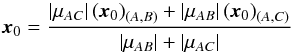 (24)denoted as the mean of the cusp position reconstructed from (A,B) and (A,C) and obtain that, in the symmetric case, the mean yields the most accurate approximation of the critical curve, while in the asymmetric case, the approximation using (A,C) is the most accurate.
Comparing Fig. 12b with the theoretical statements of Sect. 3.2, we verify that the fold critical point obtained from the evaluation of (A,B) as fold configuration lies within the parabolic approximation of the critical curve obtained from (A,B) as part of a cusp configuration. In this case, d(xA,xc) ≈ 3″ <d(xA,xf) ≈ 6.5″, so that we expect the fold reconstruction to be less accurate than the cusp one (see Sect. 3.2). Using the orthogonality assumption, we observe that the reconstruction of the fold position and the slope of the critical curve achieves the same level of accuracy as the reconstruction of the critical curve for the nearby cusp. Hence, it is possible to build a fold configuration from the images with the shortest distance in a cusp configuration and thereby obtain additional information on the properties of the critical curve at the fold point. This also implies that a cusp configuration in which image C is not observable cannot be distinguished from a fold configuration.
5. Conclusion
In this paper, we set the theoretical foundations of the model-independent characterisation of strong gravitational lenses by using the complete set of observables that can be employed in the leading order approach, and we generalised the equations developed in Wagner & Bartelmann (2016). We showed that the latter are retrieved from the generalised equations by employing symmetry assumptions, neglecting the information contained in the orientation angles of the images. We extended the analysis of biases started in Wagner & Bartelmann (2016) for multiple images of point-like sources in elliptical lens models with multiple images of extended sources approximated by the quadrupole moment of their intensity distribution. Furthermore, we found that the critical point and the slope of the critical curve can even be determined in cases of overlapping images and that the quadrupole moment is a well-suited observable even in cases of non-elliptical isocontours.
Analysing the bias introduced by a Taylor-expanded lensing potential in the vicinity of a point on the critical curve, we conclude the following:
-
The deviation in the reconstruction of fold and cusp critical pointsis below 5′′ for multiple images closer than 30% ofthe (effective) Einstein radius in a cluster scale NFW and SIE lens.
-
Breaking the mass-sheet degeneracy at a reasonable accuracy in such lenses can only be achieved in a small range of distance between the images close to a cusp using the symmetry assumptions stated in Wagner & Bartelmann (2016).
-
Using the symmetry assumption to retrieve
at a fold and including the orientation angles of the images to obtain , the ratios of potential derivatives and the slope of the critical curve at a fold are reconstructed with accuracies above 85% for relative image distances over 40% of the (effective) Einstein radius in the NFW and the SIE lens. -
Close to a cusp in the SIE lens, including the orientation angles yields more accurate ratios of potential derivatives and the symmetry assumption of Wagner & Bartelmann (2016) is only superior for the reconstruction of the cusp point from an image configuration whose source lies on the symmetry axis connecting the lens centre and the cusp in the caustic. The most accurate reconstruction of the properties of the critical curve at a cusp by a general (asymmetric) image configuration is obtained using the central image close to the cusp and the image farthest away from it. The ratio
is reconstructed with an accuracy above 86% for distances of the central image to the cusp up to 22% of the effective Einstein radius. Instead, has a much lower accuracy in the range of 75%, together yielding an accuracy above 80% for the slope if the central image is closer to the cusp than 15% of the effective Einstein radius. -
In a general (asymmetric) image configuration at a cusp, the two images closest to each other can be treated as a fold configuration and additional information on the slope and the position of the fold point can be obtained with the same level of accuracy as for the cusp.
Next, we plan to analyse multiple images in the HERA cluster, Meneghetti et al. (2017), in order to test the applicability of our approach in a realistic galaxy cluster scale simulation. Using this simulation, we will also investigate the uncertainty of the (ratios of) potential derivatives and the critical point positions due to observational imprecisions (noise and the convolution by the point-spread-function) and the validity of the assumption that intrinsic source properties are negligible.
This is the resolution of the HERA cluster, which is employed in all simulations to treat them on equal terms.
Acknowledgments
I am grateful to Matthias Bartelmann and Rüdiger Vaas for their strong support. I wish to thank Mauricio Carrasco, Agnese Fabris, Matteo Maturi, Sven Meyer, Björn-Malte Schäfer, Gregor Seidel, Nicolas Tessore, and the anonymous referee for helpful comments and discussions, and gratefully acknowledge the support by the Deutsche Forschungsgemeinschaft (DFG) WA3547/1-1.
References
- Bartelmann, M. 1996, A&A, 313, 697 [NASA ADS] [Google Scholar]
- Bartelmann, M., & Schneider, P. 2001, Phys. Rep., 340, 291 [NASA ADS] [CrossRef] [Google Scholar]
- Bertin, E., & Arnouts, S. 1996, A&AS, 117, 393 [NASA ADS] [CrossRef] [EDP Sciences] [Google Scholar]
- Graham, A. W., & Driver, S. P. 2005, PASA, 22, 118 [NASA ADS] [CrossRef] [Google Scholar]
- Kaiser, N., Squires, G., & Broadhurst, T. 1995, ApJ, 449, 460 [NASA ADS] [CrossRef] [Google Scholar]
- Meneghetti, M., Natarajan, P., Coe, D., et al. 2017, MNRAS, submitted [arXiv:1606.04548] [Google Scholar]
- Navarro, J. F., Frenk, C. S., & White, S. D. M. 1996, ApJ, 462, 563 [NASA ADS] [CrossRef] [Google Scholar]
- Petters, A. O., Levine, H., & Wambsganss, J. 2001, Singularity Theory and Gravitational Lensing, Progress in Mathematical Physics, 21 (Birkhäuser) [Google Scholar]
- Refregier, A., & Bacon, D. 2003, MNRAS, 338, 48 [NASA ADS] [CrossRef] [Google Scholar]
- Schneider, P., Ehlers, J., & Falco, E. E. 1992, Gravitational Lenses, Astronomy and Astrophysics Library (New York: Springer) [Google Scholar]
- Seitz, C., & Schneider, P. 1995, A&A, 297, 287 [NASA ADS] [Google Scholar]
- Wagner, J., & Bartelmann, M. 2016, A&A, 590, A34 [NASA ADS] [CrossRef] [EDP Sciences] [Google Scholar]
Appendix A: Influence of source properties
To show the influence of the source properties on the image observables, we use Eq. (4.12) from Bartelmann & Schneider (2001) as a starting point 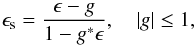 (A.1)where ϵ and ϵs are the complex variables representing the two-dimensional ellipticities of the image(s) and the source, respectively, and g is the complex variable representing the two-dimensional reduced shear
 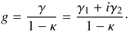 (A.2)In the following, we derive the influence of the source properties for | g | ≤ 1. The case | g | > 1 is analogous. Expressing the shear components γ1 and γ2 and the convergence κ in potential derivatives, we obtain
 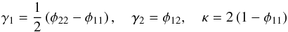 (A.3)such that | g | = 1 at the critical curve. Transforming the complex variables ϵ,ϵs,g into their polar representation, we can express the absolute value and the argument of ϵ as
  Hence, as | g | → 1 and x2 → 0,
  (A.6)In the same limit, the argument ϕϵ, which also represents the orientation angle of the semi-major axis of an image becomes aligned with the orientation of the shear, ϕg, as ϕz → 0.
Appendix B: Derivation for the fold case
For the following derivations, we rely on Chap. 6 of Schneider et al. (1992). Setting the derivative of the Taylor-expanded lensing potential to zero, we arrive at the lensing equations 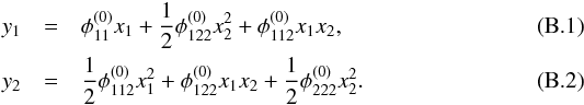 To leading order, Schneider et al. (1992) obtain that two images A and B close to the critical curve have the same x1-coordinate and their distance to the critical curve, measured along x2, is half of their mutual distance. Employing these results and the fact that A and B have the same source coordinates (y1,y2), we eliminate the latter and, without loss of generality, xB to obtain
 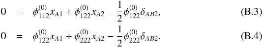 To eliminate the unknown xA1 and xA2, we insert the Taylor expansions
  for the first two terms on the right-hand sides of Eqs. (B.3)and (B.4)
 Then, we connect the distortion matrix of A with the quadrupole moment obtained from the image observables rA and ϕA. As rA and ϕA do not depend on a overall length scale, but the potential derivatives are still subject to that degeneracy, we scale them by
  , which yields
  In this step, we assume that both images are close enough to the critical curve that intrinsic ellipticities are negligible compared to the distortions caused by lensing. Inserting Eqs. (B.9)and (B.10)into Eqs. (B.7)and (B.8), we arrive at Eqs. (3)and (4).
The coordinates of the images with respect to the critical curve are obtained by the entries of the distortion matrix and Eqs. (B.5)and (B.6).  inserting Eqs. (3)and (4)for the ratios of potential derivatives on the right-hand sides.
Appendix C: Derivation for the cusp case
Analogously to Appendix B, the ratios of potential derivatives of the cusp case can be retrieved. The lensing equations of the Taylor-expanded potential read  Eliminating the source coordinates and using the Taylor expansions
  we arrive at
  if we also assume that the flexion term
  is small compared to the other terms in the last bracket on the right-hand side of Eq. (C.6)and can thus be neglected. Replacing B by C, we obtain the lensing equations for the image pair A and C. Replacing the second-order potential derivatives at the image positions by Eqs. (B.9)and (B.10)(or its negative in case of a positive cusp configuration), Eqs. (C.5) and (C.6) yield Eqs. (8)and (9).
From Eq. (C.5), we determine the angle that δAB has with the x1-axis of the cusp coordinate system, α, such that we can express δAi1 and δAi2, i = B,C as  where we also used the opening angle between δAB and δAC, denoted as αA.
The value of α is determined by first inserting  from Eq. (C.3)into Eq. (C.5), replacing δAB1 and δAB2 by Eq. (C.7)and then numerically solving the resulting equation
 (C.9)where the orientation angles between the semi-major axis of images A and B are measured with respect to δAB and are called
  and
and  , respectively (see Fig. 1b).
For the coordinates of xA, we use the flux ratio that is equal to the inverse of the respective ratio of distortion matrix determinants. Expressing the determinant of B by that of A and scaling all potential derivatives by yields  (C.10)with
  given by Eq. (12). Solving Eq. (C.10)for xA2 yields Eq. (11). The value of xA1 in Eq. (10)is then obtained by combining Eq. (B.10)(or its negative in the case of a positive cusp configuration) with Eq. (C.4)scaled by :
  (C.11)The time delay is calculated from the difference of the lensing potentials ΔφAB = φ(y,xA)−φ(y,xB). To leading order in the
Taylor expansion this potential difference reads  (C.12)Inserting Eqs. (C.1)and (C.2), subsequently Eqs. (C.3)and (C.4)and Eqs. (B.9)and (B.10), we arrive at Eq. (9), noting that t = ΔφΓd/c.
Appendix D: Derivation of Eq. (14)
As shown in Schneider et al. (1992), placing a source at y = (ys,0), its image positions of A and B in the coordinate system of the cusp configuration are given by  so that their enclosed fold critical point is located at
  (D.3)The approximation of the critical curve as a parabola along the x1-axis reads
  (D.4)using mc of Eq. (13), such that the x2-coordinate at xf1 reads
  (D.5)Employing xf2 of Eqs. (D.3)and (D.5)yields the expression for Δx2 = xc2−xf2 of Eq. (14).
All Figures
|
Fig. 1 Coordinate systems and definitions of observables for two images close to a fold critical point a) and three images close to a cusp critical point b). The thick black line in a) and parabola in b) show the approximation of the critical curve in the vicinity of the images. The fold critical point under analysis in a) is located at the crossing of the critical curve and the connection line of image A and B. The cusp critical point in b) is the vertex of the parabola. |
| In the text | |
|
Fig. 2 Analysis of the observables in three images d)–f) determines whether to apply the fold or cusp equations and where the source is located with respect to the folds and cusp a)–c): a fold configuration a) and e) shows two highly symmetric images, A, B, with larger separation to the third image, C, less magnified than A, B. In a cusp configuration b) and e), c) and f), A is highly magnified compared to B and C because it can be considered an overlay of two images generated by lensing at the upper and the lower fold which unite at the cusp point. Image shapes are neglected in these graphs, but high and low absolute values of magnifications are indicated by dark and light grey values, respectively. |
| In the text | |
|
Fig. 3 Comparison between the approximations of the critical curve as a parabola (cusp) or a line (fold) for a given source position a) shows that the fold critical point always lies below the cusp critical point in the image plane d). Depending on the distance of the source to the caustic a)–c) and the images to the critical curve d)–f), the fold approximation is more precise than the cusp approximation b) and e) or vice versa c) and f). Image C, not being relevant for the argument, is omitted here. |
| In the text | |
|
Fig. 4 Two-dimensional logarithmic intensity distribution of two images close to the radial critical curve, saddle point image B (left), maximum close to the lens centre A (right), critical curve (red), and centre of the lens (red cross). The plots at the right and bottom show vertical and horizontal intensity profiles through the critical point between A and B (red dot). |
| In the text | |
|
Fig. 5 Two-dimensional logarithmic intensity distribution of the four images generated by an SIE. The saddle point image A and the two minima B and C to the right of the lens centre (red cross) are used as cusp configuration, and A and B as configuration close to a fold (red dot). The plots at the right and bottom show vertical and horizontal intensity profiles through the critical point between A and B (red dot). |
| In the text | |
|
Fig. 6 Evaluation of the NFW profile: deviation of the reconstructed critical point from the true one, as defined in Eq. (23), dependent on the (observable) relative distance between the intensity mean of the two images a). Accuracy of Eq. (2)dependent on the same distance between images A and Bb). |
| In the text | |
|
Fig. 7 Evaluation of the NFW profile: ratio of Eq. (3)divided by the true value for image A (black solid line) and image B (red dashed line) for a low SExtractor threshold a); an intermediate threshold b); and a high threshold c). Vertical dotted lines indicate the minimum distance at which A and B are thresholded as two separate objects. The grey-shaded area marks 10% deviation from the true ratio. |
| In the text | |
|
Fig. 8 Evaluation of the SIE profile (fold): deviation of the reconstructed critical point from the true one, as defined in Eq. (23), dependent on the (observable) relative distance between the intensity mean of the two images a). Accuracy of Eq. (2)dependent on the same distance between images A and Bb). |
| In the text | |
|
Fig. 9 Evaluation of the SIE profile (fold): ratio of Eq. (4)divided by the true value for image A (black solid line) and image B (red dashed line) a). Ratio of Eq. (3)for image A and B and for both images under the symmetry assumption that their orientation is orthogonal to the critical curve (blue dotted line, green dash-dotted line) b). Slope of the critical curve, Eq. (5), at the fold using the ratios obtained in a) and b) c). The grey-shaded area marks 10% deviation from the true ratio. |
| In the text | |
|
Fig. 10 Evaluation of the SIE profile (cusp): deviation of the reconstructed critical point from the true one dependent on the (observable) relative distance between the intensity mean of the two images A and B using the pair (A,B) (black solid line), the pair of positive parity images (B,C) (red dashed line) or the pair (A,B) with the symmetry assumption that image orientation angles are parallel to the critical curve at the cusp (blue, dash-dotted line) a). Using (A,C) yields the same result as (A,B) because the source lies on the symmetry axis between B and C. The accuracy of Eq. (7)dependent on the same distance between images A and Bb) and accuracy of the analogue to Eq. (7) under the symmetry assumption stated in Wagner & Bartelmann (2016)c). |
| In the text | |
|
Fig. 11 Evaluation of the SIE-profile (cusp): ratio of Eq. (8)divided by the true value for the same configurations of image pairs and the symmetry assumption as in Fig. 10. The result for (A,B) (black solid line) coincides with the one for (B,C) (red dashed line) a). The ratio of Eq. (9)divided by the true value b). The slope of the critical curve at the cusp, Eq. (13), using the ratios obtained in a) and b) c). The grey-shaded area indicates a 10% deviation from the true ratio. |
| In the text | |
|
Fig. 12 Evaluation of the SIE profile (cusp): reconstruction of the critical curve close to a cusp for a symmetric image configuration a) and for an asymmetric image configuration b). For a) and b), the y1-value of the sources is the same, y2 varied. The symmetry axis through the lens centre (black line) is drawn to better visualise the location of the cusp point (crossing of black line and red curve) and to compare it to the vertex positions (blue, yellow and green dots) for the different reconstructions, marking the reconstructed cusp point. The reconstruction of the fold point between A and B is also shown (red dot). Inset: detail of the cusp position reconstruction. |
| In the text | |
Current usage metrics show cumulative count of Article Views (full-text article views including HTML views, PDF and ePub downloads, according to the available data) and Abstracts Views on Vision4Press platform.
Data correspond to usage on the plateform after 2015. The current usage metrics is available 48-96 hours after online publication and is updated daily on week days.
Initial download of the metrics may take a while.