| Issue |
A&A
Volume 601, May 2017
|
|
|---|---|---|
| Article Number | A14 | |
| Number of page(s) | 90 | |
| Section | Stellar structure and evolution | |
| DOI | https://doi.org/10.1051/0004-6361/201628429 | |
| Published online | 21 April 2017 | |
Ap stars with resolved magnetically split lines: Magnetic field determinations from Stokes I and V spectra⋆,⋆⋆
Joint ALMA Observatory & European Southern Observatory, 3107 Alonso de Cordova, Santiago, Chile
e-mail: This email address is being protected from spambots. You need JavaScript enabled to view it.
Received: 3 March 2016
Accepted: 26 September 2016
Abstract
Context. Some Ap stars that have a strong enough magnetic field and a sufficiently low v sini show spectral lines resolved into their magnetically split components.
Aims. We present the results of a systematic study of the magnetic fields and other properties of those stars.
Methods. This study is based on 271 new measurements of the mean magnetic field modulus ⟨ B ⟩ of 43 stars, 231 determinations of the mean longitudinal magnetic field ⟨ Bz ⟩ and of the crossover ⟨ Xz ⟩ of 34 stars, and 229 determinations of the mean quadratic magnetic field ⟨ Bq ⟩ of 33 stars. Those data were used to derive new values or meaningful lower limits of the rotation periods Prot of 21 stars. Variation curves of the mean field modulus were characterised for 25 stars, the variations of the longitudinal field were characterised for 16 stars, and the variations of the crossover and of the quadratic field were characterised for 8 stars. Our data are complemented by magnetic measurements from the literature for 41 additional stars with magnetically resolved lines. Phase coverage is sufficient to define the curve of variation of ⟨ B ⟩ for 2 of these stars. Published data were also used to characterise the ⟨ Bz ⟩ curves of variation for 10 more stars. Furthermore, we present 1297 radial velocity measurements of the 43 Ap stars in our sample that have magnetically resolved lines. Nine of these stars are spectroscopic binaries for which new orbital elements were derived.
Results. The existence of a cut-off at the low end of the distribution of the phase-averaged mean magnetic field moduli ⟨ B ⟩ av of the Ap stars with resolved magnetically split lines, at about 2.8 kG, is confirmed. This reflects the probable existence of a gap in the distribution of the magnetic field strengths in slowly rotating Ap stars, below which there is a separate population of stars with fields weaker than ~2 kG. In more than half of the stars with magnetically resolved lines that have a rotation period shorter than 150 days, ⟨ B ⟩ av > 7.5 kG, while those stars with a longer period all have ⟨ B ⟩ av < 7.5 kG. The difference between the two groups is significant at the 100.0% confidence level. The relative amplitudes of variation of the mean field modulus may tend to be greater in stars with Prot > 100 d than in shorter period stars. The root-mean-square longitudinal fields of all the studied stars but one is less than one-third of their phased-average mean field moduli, which is consistent with the expected behaviour for fields whose geometrical structure resembles a centred dipole. However, moderate but significant departures from the latter are frequent. Crossover resulting from the correlation between the Zeeman effect and the rotation-induced Doppler effect across the stellar surface is definitely detected in stars with rotation periods of up to 130 days and possibly even up to 500 days. Weak, but formally significant crossover of constant sign, has also been observed in a number of longer period stars, which could potentially be caused by pulsation velocity gradients across the depth of the photosphere. The quadratic field is in average ~1.3 times greater than the mean field modulus and both of those moments vary with similar relative amplitudes and almost in phase in most stars. Rare exceptions almost certainly have unusual field structures. The distribution of the known values and lower limits of the rotation periods of the Ap stars with magnetically resolved lines indicates that for some of them, Prot must almost certainly reach 300 yr or possibly even much higher values. Of the 43 Ap stars that we studied in detail, 22 are in binary systems. The shortest orbital period Porb of those systems is 27 days. For those non-synchronised Ap binaries for which both the rotation period and the orbital period, or meaningful lower limits thereof, are reliably determined, the distribution of the orbital periods of the systems in which the Ap star has a rotation period that is shorter than 50 days is different from its distribution for those systems in which the rotation period of the Ap star is longer, at a confidence level of 99.6%. The shortest rotation and orbital periods are mutually exclusive: all but one of the non-synchronised systems that contain an Ap component with Prot < 50 d, have Porb > 1000 d.
Conclusions. Stars with resolved magnetically split lines represent a significant fraction, of the order of several percent, of the whole population of Ap stars. Most of these stars are genuine slow rotators, whose consideration provides new insight into the long-period tail of the distribution of the periods of Ap stars. Emerging correlations between rotation periods and magnetic properties provide important clues for the understanding of the braking mechanisms that have been at play in the early stages of stellar evolution. The geometrical structures of the magnetic fields of Ap stars with magnetically resolved lines appear in general to depart slightly, but not extremely, from centred dipoles. However, there are a few remarkable exceptions, which deserve further consideration. Confirmation that pulsational crossover is indeed occurring at a detectable level would open the door to the study of non-radial pulsation modes of degree ℓ, which is too high for photometric or spectroscopic observations. How the lack of short orbital periods among binaries containing an Ap component with magnetically resolved lines is related to their (extremely) slow rotation remains to be fully understood, but the very existence of a correlation between the two periods lends support to the merger scenario for the origin of Ap stars.
Key words: stars: chemically peculiar / stars: magnetic field / stars: rotation / binaries: general / stars: oscillations
Based on observations collected at the European Southern Observatory, Chile (ESO Programmes 56.E-0688, 56.E-0690, 57.E-0557, 57.E-0637, 58.E-0155, 58.E-0159, 59.E-0372, 59.E-0373, 60.E-0564, 60.E-0565, 61.E-0711, and Period 56 Director Discretionary Time); at Observatoire de Haute Provence (CNRS), France; at Kitt Peak National Observatory, National Optical Astronomy Observatory (NOAO Prop. ID: KP2442; PI: T. Lanz), which is operated by the Association of Universities for Research in Astronomy (AURA) under cooperative agreement with the National Science Foundation; and at the Canada-France-Hawaii Telescope (CFHT), which is operated from the summit of Mauna Kea by the National Research Council of Canada, the Institut National des Sciences de l’Univers of the Centre National de la Recherche Scientifique of France, and the University of Hawaii. The observations at the Canada-France-Hawaii Telescope were performed with care and respect from the summit of Mauna Kea, which is a significant cultural and historic site.
Table 7 is only available at the CDS via anonymous ftp to cdsarc.u-strasbg.fr (130.79.128.5) or via http://cdsarc.u-strasbg.fr/viz-bin/qcat?J/A+A/601/A14
© ESO, 2017
1. Introduction
Babcock (1960) was the first to report the observation of spectral lines resolved into their Zeeman-split components by a magnetic field in a star other than the Sun: i.e. the B9p star HD 215441 (since then known as Babcock’s star)1. As Babcock realised, the observations of sharp, resolved line components implies that the star has a low projected equatorial velocity v sini, and that its magnetic field is fairly uniform. From consideration of the wavelength separation of the resolved line components, Babcock inferred that the average over the visible stellar disk of the modulus of its magnetic field (the mean magnetic field modulus) is of the order of 34 kG. Quite remarkably, more than half a century later, this still stands as the highest mean magnetic field modulus measured in a non-degenerate star.
By the end of 1970, Preston had identified eight more Ap stars with magnetically resolved lines (see Preston 1971, and references therein). Preston recognised that the mean magnetic field modulus is fairly insensitive to the geometry of the observation, contrary to the mean longitudinal magnetic field (i.e. the average over the visible stellar hemisphere of the line-of-sight component of the magnetic vector). This field moment, which is determined from the analysis of the circular polarisation of spectral lines, is the main diagnostic of Ap star magnetic fields, of which the largest number of measurements have been published. The interest of combining measurements of the mean longitudinal field and mean field modulus to derive constraints on the structure of stellar magnetic fields was also recognised early on. However, for the next two decades, Ap stars with magnetically resolved lines, which represented only a very small subset of all Ap stars, remained hardly more than a curiosity, to which very little attention was paid.
Yet these stars are especially worth studying for various reasons:
-
Thanks to its low sensitivity to the geometry of the observation,the mean magnetic field modulus is the observable that bestcharacterises the intrinsic strength of the stellar magnetic field.By contrast, the mean longitudinal magnetic field dependscritically on the line of sight, hence on the location of the observer.
-
Furthermore, the determination of the mean field modulus from measurements of the wavelength separation of the resolved components of Zeeman-split lines is not only very simple and straightforward, but also, more importantly, it is model free and almost approximation free (see Sect. 3.1).
-
As already mentioned, the possibility of complementing spectropolarimetry-based determinations of magnetic field moments (most frequently, of the mean longitudinal field) with mean field modulus measurements, and of considering how both vary as the stars rotate, allows one to derive significant constraints on the structure of the stellar field.
-
Ap stars with resolved magnetically split lines, in their majority, have (very) long rotation periods (as discussed in more detail in Sect. 5.5). They represent extreme examples of the slow rotation that is characteristic of Ap stars in general (compared to normal main-sequence stars of similar temperature). This makes them particularly well suited to investigating the mechanisms through which Ap stars have managed during their past evolution to shed large amounts of angular momentum.
These considerations prompted us around 1990 to initiate a large comprehensive effort to study Ap stars with resolved magnetically split lines systematically. Mathys et al. (1997, hereafter Paper I gave an extensive account of the results obtained from the analysis of the observations obtained between May 1988 and August 1995. By then, 42 Ap stars with magnetically resolved lines were known, of which 30 had been discovered since 1988; all but one of these discoveries were made in the framework of our project. Paper I presented 752 measurements of the mean magnetic field modulus of 40 of these 42 stars. Their analysis led to a large number of new results:
-
new or improved rotation periods, or lower limits of such periods;
-
variation curves of the mean magnetic field modulus;
-
detection of radial velocity variations indicative of binarity;
-
statistical constraints on the properties of Ap stars with magnetically resolved lines, in particular, with respect to their magnetic fields.
We do not present a more detailed summary of those results here, since they are significantly updated and augmented in the rest of this paper.
In 1995, we started a programme of systematic spectropolarimetric observations of Ap stars with magnetically resolved lines, with a view towards deriving additional constraints on the properties of their magnetic fields from analysis of the circular polarisation of their spectral lines. Here we present the results of this complementary study, which also includes new magnetic field modulus measurements obtained from additional high-resolution spectroscopic observations performed during the same time interval, that is, between October 1995 and September 1998. Although for a number of the stars of our sample, more recent high-resolution spectroscopic observations in natural light and/or spectropolarimetric observations are available in the archives of several observatories, we do not consider them in this paper for the sake of the homogeneity of the analysed data. This homogeneity is particularly important to minimise ambiguities in the study of small-amplitude, long-term variations (on timescales of several years). However, we do fully take new data that have already been published into account, albeit making sure that these data can always be distinguished from our own measurements.
Nowadays, the most detailed and accurate determinations of the geometrical structure of Ap star magnetic fields are achieved via application of the techniques of Zeeman-Doppler imaging or magnetic Doppler imaging (e.g. Piskunov & Kochukhov 2002). However, the vast majority of Ap stars with resolved magnetically split lines do not lend themselves to the application of these techniques because their projected equatorial velocity v sini is in general too small. In this context, the moment technique (Mathys 1988) represents a powerful alternative that allows one to characterise the main magnetic properties of the observed stars with a small set of quantities (magnetic field moments) and their variations with rotation phase. This numeric information can then be subjected to statistical analysis; generic properties of the subset of Ap stars with magnetically resolved lines, and possible exceptions, can be inferred. This is the approach that we have followed in this work. The moments that we have considered characterise the mean intensity of the magnetic field over the stellar surface and its component along the line of sight; the spread of the distribution of the local field values across the disk of the star; and the existing correlations between the magnetic field structure and stellar velocity fields that are organised on large scales.
In order to strengthen the statistical significance of our conclusions, we included, whenever possible while maintaining sufficient quality and uniformity of the analysed data, results from other groups that are available in the literature. In particular, we tried to keep track of all the Ap stars with magnetically resolved lines that have been discovered since 1998. We reckon that at present, 84 Ap stars are known to show magnetically resolved lines. This represents 2.3% of the total number of Ap stars in Renson & Manfroid’s (2009) catalogue. As these authors stress, this catalogue is not homogeneous, nor is the set of known Ap stars with magnetically resolved lines. The latter, which was assembled from different sources, is certainly biassed towards the brightest stars, and it contains a disproportionate number of stars with southern declination, 68 out of 84 (81%). Thus 2.3% should be regarded at best as a moderately meaningful lower limit to the actual fraction of Ap stars showing resolved magnetically split lines. The Elkin et al. (2012) estimate that this fraction is a little less than 10% may be more realistic, given that it is based on a systematic observational study of a reasonably unbiassed sample of stars. However, this sample is restricted to (fairly) cool Ap stars. It is probably safe to assume that the actual fraction of Ap stars whose spectral lines are resolved in their magnetically split components is somewhere between 2.3% and 10%. Even if this number is not exactly known, it leaves little doubt about the fact that, contrary to the feeling that prevailed until two decades ago, Ap stars with magnetically resolved lines are not isolated odd specimens, but that instead they constitute a very significant subset of the Ap star population.
The main properties of the 43 stars for which new magnetic field measurements are presented in this paper are summarised in Table 1. Columns 1 to 4 give, in order, their HD (or HDE) number, an alternative identification, the visual magnitude V, and the spectral type according to the Catalogue of Ap, HgMn and Am stars (Renson & Manfroid 2009). For those stars whose rotation period is known, or is determined in this paper, its value appears in Col. 5, with the time origin adopted to phase the magnetic data in Col. 7, and the property (e.g. specific extremum of a magnetic field moment) from which this phase was defined in Col. 8. For the remaining stars, a lower limit of the period is given in Col. 5 whenever it could be set. Columns 6 and 9 identify the reference from which the period and phase origin information is extracted, respectively; when those parameters were determined in the present work, the corresponding entry is left blank.
The other 41 Ap stars with magnetically resolved lines that are currently known are listed in Table 2. Its structure is similar to that of Table 1, except for an additional column (Col. 5) giving the reference of the paper in which the presence of magnetically resolved lines was first reported.
Ap stars with resolved magnetically split lines: stars for which new measurements of the mean magnetic field modulus are presented in this paper.
Ap stars with resolved magnetically split lines: stars with magnetic measurements from the literature.
The new observations whose analysis is reported in this paper are introduced in Sect. 2. Section 3 describes how they were used for determination of the magnetic field moments of interest and the stellar radial velocities. The results of these measurements are presented in Sect. 4, which also explains how the variations of the different derived quantities were characterised. The implications of the new data obtained in this work for our knowledge of the physical properties of Ap stars are discussed in Sect. 5, and some general conclusions are drawn in Sect. 6. A number of specialised issues that deserved more detailed consideration outside the main flow of the paper were moved to the appendices. These include notes on the individual stars for which new magnetic field measurements were obtained (Appendix A), a revision of older determinations of the mean quadratic magnetic field (Appendix B), and the mathematical formalism underlying a proposal for a new physical mechanism to generate the crossover effect in spectral lines observed in circular polarisation (Appendix C).
2. Observations
There are two types of new observations presented in this paper as follows:
-
additional high-resolution (R = λ/ Δλ ~ 7 × 10⁴–1.2 × 10⁵) spectra recorded in natural light, similar to the data of Paper I;
-
lower resolution (R ~ 3.9 × 10⁴) circularly polarised spectra.
The unpolarised spectra were obtained between October 1995 and September 1998 with a subset of the telescope and instrument combinations used in Paper I:
-
the European Southern Observatory’s (ESO) Coudé EchelleSpectrograph (CES) in its Long Camera (LC) configuration, fedby the 1.4 m Coudé Auxiliary Telescope (CAT);
-
the AURELIE spectrograph of the Observatoire de Haute-Provence (OHP), fed by the 1.5 m telescope;
-
Kitt Peak National Observatory’s (KPNO) Coudé spectrograph at the 0.9 m Coudé feed;
-
the f/ 4 Coudé spectrograph (Gecko) of the 3.6 m Canada-France-Hawaii Telescope (CFHT) at Mauna Kea;
-
the ESO Multi-Mode Instrument (EMMI) in its high-resolution échelle mode, fed by the 3.5 m New Technology Telescope.
The observing procedures that were followed and the instrumental configurations that were used have been described in more detail in Paper I. In April 1998, the Long Camera (LC) of the CES was decommissioned and replaced by the Very Long Camera (VLC; Kürster 1998). We used the VLC (with CCD #38) for the final three observing runs of 1998. We set the width of the entrance slit of the CES so as to achieve the same resolving power as with the LC configuration of our previous runs (with CCD #34). Thus, in practice, the VLC+CCD #38 and LC+CCD #34 configurations of the CES can be regarded as equivalent for our purpose: we shall not distinguish them further in this paper.
The full list of the configurations that were used to record the high-resolution, unpolarised spectra analysed here and in Paper I appears in Table 3. The third column gives the symbol used to distinguish them in the figures of Appendix A. We used the same identification numbers and symbols as in Paper I. As in the latter, configurations that are practically equivalent were given the same identification.
Table 4 lists the dates of the individual observing runs (totalling 50 nights) partly or entirely devoted to the acquisition of the new high-resolution spectra discussed in this paper. Columns 1 and 2 give the start and end date of the run (in local time of the observatory, from the beginning of the first night to the end of the last night). The identification number assigned to the instrumental configuration used during the run (see Table 3) appears in Col. 3. Each instrumental configuration is summarised in Cols. 4 to 7, which list, in order, the observatory where the observations were performed, and the telescope, instrument, and detector that were used.
All data were reduced using the ESO image processing package MIDAS (Munich Image Data Analysis System), performing the same steps as described in Paper I, except for the CFHT Gecko spectra, which were reduced with IRAF (Image Reduction and Analysis Facility). For a more detailed description of the reduction of the EMMI échelle spectra and, in particular, of their wavelength calibration, see Mathys & Hubrig (2006).
All the spectropolarimetric data presented here were obtained with the ESO Cassegrain Echelle Spectrograph (CASPEC) fed by the ESO 3.6 m telescope. The configuration that was used is the same as specified by Mathys & Hubrig (1997) for the spectra recorded since 1995. Data reduction was also as described in that reference. The CASPEC spectropolarimetric observations of this paper were performed on 28 different nights spread between February 1995 and January 1998.
3. Magnetic field and radial velocity determinations
3.1. Mean magnetic field modulus
The mean magnetic field modulus ⟨ B ⟩ is the average over the visible stellar disk of the modulus of the magnetic field vector, weighted by the local emergent line intensity. In the present study, as in Paper I, the mean magnetic field modulus was determined from measurement of the wavelength separation of the magnetically split components of the Fe ii λ 6149.2 line, a Zeeman doublet, by application of the following formula: 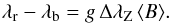 (1)In this equation, λr and λb are the wavelengths of the red and blue split line components, respectively; g is the Landé factor of the split level of the transition (g = 2.70; Sugar & Corliss 1985);
  , with k = 4.67 × 10⁻¹³ Å-1 G-1; and λ0 = 6149.258 Å is the nominal wavelength of the considered transition.
The motivation for the usage of Fe ii λ 6149.2 as the diagnostic line, the involved limitations and approximations, and the methods used to measure the wavelengths of its split components have been exhaustively described in Paper I. Like in Paper I, the actual measurements of λr and λb are carried out either by direct integration of the split line component profiles, or by fitting them (and possible blending lines) by multiple Gaussians, as described by Mathys & Lanz (1992).
The difficulty in estimating the uncertainties affecting our mean magnetic field modulus measurements was explained in Paper I (see in particular Sect. 6, which also includes a detailed discussion of the systematic errors). For the stars that were studied in that paper, we adopt here the same values of these uncertainties. For HD 47103, HD 51684, and HD 213637, which did not feature in Paper I, the way in which the measurement undertainties were estimated is described in the respective sections of Appendix A.
3.2. Mean longitudinal magnetic field, crossover, and mean quadratic magnetic field
The moment technique (Mathys 1988, 1989; see also Mathys 2000) was used to extract, from the CASPEC Stokes I and V spectra, three parameters characterising the magnetic fields of the studied stars: the mean longitudinal magnetic field, the crossover, and the quadratic field. Hereafter, we give an operational definition of these parameters, based on a description of their determination. We then briefly discuss their physical interpretation. This approach is slightly different from the one we used in previous papers. Adopting this approach is justified by the fact that, as becomes apparent later (see in particular Sect. 5.3), some of the magnetic parameters that we consider may correspond to different physical processes in different stars.
Let λI be the wavelength of the centre of gravity of a spectral line observed in the Stokes parameter I. In what follows, we refer to λI as the line centre. The moment of order n of the profile of this line about its centre, in the Stokes parameter X (X = I,Q,U,V), is defined as 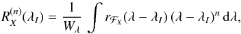 (2)where Wλ is the equivalent width of the line, and rℱX is its normalised profile in the Stokes parameter X,
 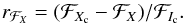 (3)The notations ℱX and ℱXc represent the integral over the visible stellar disk of the emergent intensity (in the considered Stokes parameter) in the line and the neighbouring continuum, respectively, as follows:
 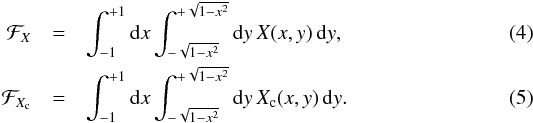 where (x,y) are the coordinates of a point on the visible stellar disk, in a reference system where the z-axis is parallel to the line of sight, the y-axis lies in the plane defined by the line of sight and the stellar rotation axis, and the unit length is the stellar radius. The integral over the wavelength in Eq. (2) extends over the whole observed line (see Mathys 1988, for details).
Observing runs and instrumental configurations: high-resolution spectra in natural light.
The mean longitudinal field ⟨ Bz ⟩ is derived from measurements of the first-order moments  of Stokes V line profiles about the respective line centre, by application of the formula (Mathys 1995a),
 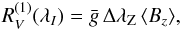 (6)where
  is the effective Landé factor of the transition. One can note that the first-order moment of the Stokes V line profile is a measurement of the wavelength shift of a spectral line between observations in opposite circular polarisations,
 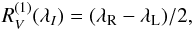 (7)where λR (resp. λL) is the wavelength of the centre of gravity of the line in right (resp. left) circular polarisation. Under some assumptions that in most cases represent a good first approximation (Mathys 1989, 1991, 1995a), ⟨ Bz ⟩ can be interepreted as being the average over the visible stellar disk of the component of the magnetic vector along the line of sight, weighted by the local emergent line intensity.
In practice, is measured for a sample of lines. The required integration, for this and the other line moments discussed below, is performed as described in Sect. 2 of Mathys (1994). Then, in application of Eq. (6), ⟨ Bz ⟩ is determined from a linear least-squares fit as a function of  , forced through the origin. Following Mathys (1994), this fit is weighted by the inverse of the mean-square error of the measurements for the individual lines,
 ![Mathematical equation: \hbox{$1/\sigma^2[\R{1}{V}]$}](/articles/aa/full_html/2017/05/aa28429-16/aa28429-16-eq128.png) . The standard error σz of the longitudinal field that is derived from this least-squares analysis is used as an estimate of the uncertainty affecting the obtained value of ⟨ Bz ⟩.
. The standard error σz of the longitudinal field that is derived from this least-squares analysis is used as an estimate of the uncertainty affecting the obtained value of ⟨ Bz ⟩.
The crossover ⟨ Xz ⟩ is derived from measurements of the second-order moments  of the Stokes V line profiles about the respective line centre, by application of the formula
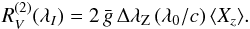 (8)The second-order moment of the Stokes V line profile is a measurement of the difference of the width of a spectral line between observations in opposite circular polarisations. Under the same assumptions as for the longitudinal field (Mathys 1995a), and as long as the only macroscopic velocity field contributing to the line profile is the stellar rotation (a condition that may not always be fulfilled; see Sect. 5.3), ⟨ Xz ⟩ can be interpreted as being the product of the projected equatorial velocity of the star, v sini, and of the mean asymmetry of the longitudinal magnetic field, ⟨ xBz ⟩. The latter is defined as the first-order moment about the plane defined by the stellar rotation axis and the line of sight of the component of the magnetic vector parallel to the line of sight, weighted by the local emergent line intensity.
In practice, is measured for a sample of lines. Then, in application of Eq. (8), ⟨ Xz ⟩ is determined from a linear least-squares fit as a function of  , forced through the origin. This fit is weighted by the inverse of the mean-square error of the measurements for the individual lines,
 ![Mathematical equation: \hbox{$1/\sigma^2[\R{2}{V}]$}](/articles/aa/full_html/2017/05/aa28429-16/aa28429-16-eq134.png) . The standard error σx of the crossover that is derived from this least-squares analysis is used as an estimate of the uncertainty affecting the obtained value of ⟨ Xz ⟩.
. The standard error σx of the crossover that is derived from this least-squares analysis is used as an estimate of the uncertainty affecting the obtained value of ⟨ Xz ⟩.
The mean quadratic field ⟨ Bq ⟩ is derived from measurements of the second-order moments  of the Stokes I line profiles about the respective line centre by application of the following formula (Mathys & Hubrig 2006):
 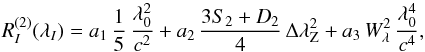 (9)where a2 = ⟨ Bq ⟩ 2. In this equation, S2 and D2 are atomic parameters characterising the Zeeman pattern of the considered transition. They are defined in terms of the coefficients
  and
and  introduced by Mathys & Stenflo (1987),
  The second-order moment of the Stokes I line profile is a measurement the spectral line width in natural light. It results from the combination of contributions of various effects: natural line width and instrumental profile (both of which cancel out in the Stokes V profiles), Doppler effect of various origins (thermal motion, stellar rotation, possibly microturbulence, or pulsation, ...), and magnetic broadening. For the interpretation of the physical meaning of ⟨ Bq ⟩, the basic assumptions are similar to those used for ⟨ Bz ⟩ and ⟨ Xz ⟩, but their relevance is somewhat different (Mathys 1995b). Mathys & Hubrig (2006) discussed in detail the physical exploitation of the information contents of via a semi-empirical approach, on which Eq. (9) is based. Within this context, ⟨ Bq ⟩ is interpreted as the square root of the sum of the following two field moments:
-
the average over the visible stellar disk of the square of themodulus of the magnetic vector, ⟨ B2 ⟩;
-
the average over the visible stellar disk of the square of the component of the magnetic vector along the line of sight,
 .
.
Both averages are weighted by the local emergent line intensity. The form adopted here for Eq. (9) is based on the assumption that  . The reason why this assumption is needed and its justification have been presented in previous works on the quadratic field (Mathys 1995b; Mathys & Hubrig 2006). The adequacy of this approximation is discussed further in Sect. 5.4.
Practical application of Eq. (9) is somewhat more complicated than for Eqs. (6) and (8). The same principle as for the latter is applied: is measured for a sample of lines and a linear least-squares fit to these data of the form given by Eq. (9) is computed. However this is now a multi-parameter fit, with three independent variables, so that three fit parameters (a1, a2, and a3) must be determined. In most studied stars, the number of diagnostic lines is of the order of 10, sometimes less, and it exceeds 20 in only one case. As a result, the derived parameters may be poorly constrained; in particular, there may be significant ambiguities between their respective contributions.
In order to alleviate the problem, we used an approach similar to that of Mathys (1995b). This approach is based on the consideration that the a2 term is the only term on the right-hand side of Eq. (9) that is expected to show significant variability with stellar rotation phase, so that the fit parameters a1 and a3 should have the same values at all epochs of observation. Accordingly, for each star that has been observed at least at three different epochs, we compute for each diagnostic line the average ![Mathematical equation: \hbox{$[\R{2}{I}]_{\rm av}$}](/articles/aa/full_html/2017/05/aa28429-16/aa28429-16-eq151.png) of the measurements of for this line at the various epochs. We derive the values of a1 and a3 through a least-squares fit of by a function of the form given in the right-hand side of Eq. (9). This fit is weighted by
of the measurements of for this line at the various epochs. We derive the values of a1 and a3 through a least-squares fit of by a function of the form given in the right-hand side of Eq. (9). This fit is weighted by ![Mathematical equation: \hbox{$1/\sigma^2\lbrace[\R{2}{I}]_{\rm av}\rbrace$}](/articles/aa/full_html/2017/05/aa28429-16/aa28429-16-eq152.png) , where
, where ![Mathematical equation: \hbox{$\sigma\lbrace[\R{2}{I}]_{\rm av}\rbrace$}](/articles/aa/full_html/2017/05/aa28429-16/aa28429-16-eq153.png) is calculated by application of error propagation to the root-mean-square errors of the individual measurements of for the considered line at the different epochs of observations. Then we use these values of a1 and a3 to compute the magnetic part of for each line and at each epoch as follows:
is calculated by application of error propagation to the root-mean-square errors of the individual measurements of for the considered line at the different epochs of observations. Then we use these values of a1 and a3 to compute the magnetic part of for each line and at each epoch as follows: ![Mathematical equation: \begin{equation} \left[\R{2}{I}\right]_{\rm mag}=\R{2}{I}-a_1\,{1\over5}\,{\lambda_0^2\over c^2}-a_3\,\ew^2\,{\lambda_0^4\over c^4}\cdot \label{eq:R2I_mag} \end{equation}](/articles/aa/full_html/2017/05/aa28429-16/aa28429-16-eq154.png) (12)Finally, we compute a linear least-squares fit, forced through the origin, of
(12)Finally, we compute a linear least-squares fit, forced through the origin, of ![Mathematical equation: \hbox{$[\R{2}{I}]_{\rm mag}$}](/articles/aa/full_html/2017/05/aa28429-16/aa28429-16-eq155.png) as a function of
as a function of  to derive ⟨ Bq ⟩, in application of the relation,
 ![Mathematical equation: \begin{equation} \left[\R{2}{I}\right]_{\rm mag}=\Hq^2\,{3S_2+D_2\over4}\,\Zeeman^2. \label{eq:Hq_av} \end{equation}](/articles/aa/full_html/2017/05/aa28429-16/aa28429-16-eq157.png) (13)This least-squares fit is weighted by the inverse of the mean-square error of the
(13)This least-squares fit is weighted by the inverse of the mean-square error of the  measurements for the individual lines at the considered epoch,
 ![Mathematical equation: \hbox{$1/\sigma^2[\R{2}{I}]$}](/articles/aa/full_html/2017/05/aa28429-16/aa28429-16-eq159.png) . The standard error σq of the mean quadratic field that is derived from this least-squares analysis is used as an estimate of the uncertainty affecting the obtained value of ⟨ Bq ⟩.
. The standard error σq of the mean quadratic field that is derived from this least-squares analysis is used as an estimate of the uncertainty affecting the obtained value of ⟨ Bq ⟩.
Previous mean quadratic field determinations (Mathys 1995b; Mathys & Hubrig 1997) were not based on Eq. (9), but on the simpler form,  (14)In other words, the dependences of on the line wavelength and equivalent width were ignored, except for the wavelength dependence appearing in the magnetic term. The obvious shortcoming of the application of Eq. (14) instead of Eq. (9) for determination of the quadratic field is that part of the wavelength dependence of , corresponding to the a1 and a3 terms of Eq. (9), is likely to end up absorbed into the a2 term of Eq. (14), rather than into its a0 term. In other words, neglecting the wavelength (and equivalent width) dependence of the non-magnetic contributions to the Stokes I line width must in general introduce systematic errors (typically, overestimates) in the determination of the mean quadratic magnetic field.
Accordingly, to be able to combine, in the most consistent way, the quadratic field data based on our previous observations with the measurements obtained from the new observations of this paper, whenever possible we used revised ⟨ Bq ⟩ values determined by application of Eq. (13) to the spectra of Mathys (1995b). These values are given in Appendix B.
This approach cannot be used for the observations of Mathys & Hubrig (1997), which for each star have been obtained at different epochs with different instrumental configurations, for which the fit parameters a1 and a3 in general have different values. On the other hand, the number of diagnostic lines in those spectra is too small for direct application of Eq. (9), so that in the rest of this paper, the values of the quadratic field derived by Mathys & Hubrig (1997) through application of Eq. (14) are used unchanged. When assessing their implications, one should keep in mind that they may in general be less accurate than the most recent determinations of the present study or the revised values derived from the older observations of Mathys (1995b).
3.3. Radial velocities
Our observations, both in natural light and in circular polarisation, were not originally meant to be used for the determination of stellar radial velocities, whether they were obtained in the framework of the present project (for this paper and Paper I) or our earlier works (Mathys 1991, 1994, 1995a,b; Mathys & Hubrig 1997). In particular, no observations of radial velocity standards were obtained in any of our observing runs. Nevertheless, most of our spectra proved extremely well suited to the determination of accurate radial velocities, as became apparent in the analysis of our data. This allowed us to report in Paper I the discovery of radial velocity variations in eight stars that were not previously known to be spectroscopic binaries, some of which had observed amplitudes that do not exceed a few km s-1. Consideration of these stars, together with the other members of our sample that were already known as binaries, suggested the possibility of a systematic difference of the lengths of orbital periods between binaries involving Ap stars with magnetically resolved lines and other Ap binaries. In view of these results, it appeared justified to exploit the potential of our data in a more systematic manner, to publish the radial velocities obtained from their analysis, and to carry out determinations of the orbital elements of the observed spectroscopic binaries whenever the number and distribution of the available measurements made it possible.
Radial velocities were determined from the new spectropolarimetric observations of this paper as well as from the similar CASPEC spectra of Mathys (1991) and Mathys & Hubrig (1997) by analysing the same sets of spectral lines as for the measurement of the mean longitudinal magnetic field. We computed a least-squares fit, forced through the origin, of the differences between the wavelength λI of their centre of gravity in Stokes I and the nominal wavelength of the corresponding transitions, λ0. This fit is weighted by the inverse of the mean-square error of the λI measurements of the individual lines. The radial velocity is derived from its slope in the standard manner. The standard deviation of the velocity that is obtained from this analysis correctly characterises the precision of the measurements, but not their accuracy. This is discussed further in Sect. 5.6.
The narrow wavelength range covered by most of our high-resolution, natural light spectra does not allow us to use a similar approach to determine radial velocities from their analyses. In these spectra, the unpolarised wavelength λI of the Fe ii λ 6149.2 line was computed by averaging the wavelengths of its blue and red split components as measured for the determination of the mean magnetic field modulus as follows:  (15)Then, the wavelength difference λI−λ0, where λ0 = 6149.258 Å is the nominal wavelength of the transition, was converted to a radial velocity value in the standard manner. The notations Wλ,b and Wλ,r refer to the equivalent widths of the measured parts of each line component. Indeed, the values of those equivalent widths depend on the limits between which the direct integration of the line was performed, or between which the multiple Gaussians were fitted to the observed profile. These limits in turn depend on line blends possibly affecting the Fe ii λ 6149.2 line. As a result, the measured equivalent widths of the split components may be significantly different from (in general, smaller than) their actual values (which would be measured in an ideal case). The approach described in this paragraph was applied to the high-resolution unpolarised spectra analysed in the present paper and to the observations presented in Paper I. A few of the latter were omitted, since they had been obtained as part of observing runs lacking absolute wavelength calibrations suitable for reliable radial velocity determinations.
Like for the mean field modulus, as the radial velocity is determined from consideration of a single line, it is not straightforward to estimate the measurement uncertainties. The discussion of this issue is postponed to Sect. 5.6.
Mean magnetic field modulus.
continued.
Mean longitudinal magnetic field, crossover, and mean quadratic magnetic field.
continued.
continued.
4. Results
4.1. Individual measurements
The results of our measurements of the mean magnetic field modulus are presented Table 5. Column 1 gives the heliocentric Julian date of mid-observation. The value of the field modulus appears in Col. 2, and the code of the instrumental configuration used for the observation (as per Table 4) is listed in Col. 3.
The values of the three magnetic field moments determined from the analysis of our CASPEC spectropolarimetric observations are given in Table 6: the mean longitudinal field in Col. 2, the crossover in Col. 4, and the mean quadratic field in Col. 6. Their standard errors appear in Cols. 3, 5, and 7, respectively. Column 8 gives the number of spectral lines that were used in their determination.
Table 7, available at the CDS, presents all the radial velocity measurements from the spectra analysed in this paper as well as from the observations of Mathys (1991), Mathys & Hubrig (1997) and Paper I. Columns 1 to 4 contain the HD or HDE number of the star, the heliocentric Julian date of the observation, the heliocentric radial velocity value, and the adopted value of its uncertainty, respectively (see Sect. 5.6).
Variation of the mean longitudinal magnetic field: least-squares fit parameters for stars with ⟨ Bz ⟩ data in this paper.
Variation of the crossover: least-squares fit parameters.
Variation of the mean quadratic magnetic field: least-squares fit parameters.
4.2. Variation curves of the moments of the magnetic field
For those stars with a known rotation period, or for which a probable value of this period could be derived with reasonable confidence, we fitted our magnetic measurements against rotation phase φ with a cosine curve, ![Mathematical equation: \begin{equation} A_B(\phi)=A_0+A_1\,\cos[2\pi\,(\phi-\phi_1)], \label{eq:fit1} \end{equation}](/articles/aa/full_html/2017/05/aa28429-16/aa28429-16-eq420.png) (16)or with the superposition of a cosine and of its first harmonic,
(16)or with the superposition of a cosine and of its first harmonic,
![Mathematical equation: \begin{eqnarray} &&A_B(\phi)=A_0+A_1\,\cos[2\pi\,(\phi-\phi_1)] +A_2\,\cos[2\pi\,(2\phi-\phi_2)]. \label{eq:fit2} \end{eqnarray}](/articles/aa/full_html/2017/05/aa28429-16/aa28429-16-eq421.png) (17)
(17)
In these formulae, AB represents any of the magnetic moments of interest (⟨ B ⟩, ⟨ Bz ⟩, ⟨ Xz ⟩, ⟨ Bq ⟩). The rotation phase is calculated using the values of the phase origin, HJD0, and of the rotation period, Prot, that appear in Table 1. The mean value A0, the amplitude(s) A1 (and A2), and the phase(s) φ1 (and φ2) of the variations are determined through a least-squares fit of the field moment measurements by a function of the form given in either Eq. (16) or (17). This fit is weighted by the inverse of the square of the uncertainties of the individual measurements.
New or revised orbital elements of spectroscopic binaries. The second row for each entry gives its standard deviation.
The forms adopted for the fit functions are the same as in our previous studies of magnetic fields of Ap stars (e.g. Mathys & Hubrig 1997). This is not an arbitrary choice in the sense that these functions generally represent well the observed behaviour of the various field moments. Nevertheless they should be considered only as convenient tools to characterise the field variations in a simple way that lends itself well to inferring statistical properties of the magnetic fields of the studied stars, but they should not be overinterpreted in terms of the actual physical properties of the field of any single object.
The results of the fits are presented in Table 8, for ⟨ B ⟩, the amplitudes are denoted as Mi, i = 0, 1, 2, and the phases are listed as φMi, i = 1, 2; Table 9, for ⟨ Bz ⟩, the amplitudes are denoted as Zi and the phases are listed as φZi; in Table 10, for ⟨ Xz ⟩, the amplitudes are denoted as Xi and the phases are listed as φXi; and in Table 11, for ⟨ Bq ⟩, the amplitudes are denoted as Qi and the phases are listed as φQi. Columns 7 to 9 of these tables give the number of degrees of freedom about the fit ν, the reduced χ2 of the fit χ2/ν, and the multiple correlation coefficient R. Fits were only computed when at least five or seven measurements of the field moment (for fits of the form given by Eqs. (16) or (17), respectively), sufficiently spread over the rotation period, were obtained for the considered star. The following criteria were applied to decide whether or not the first harmonic should be included in the fits whose results appear in Tables 8 to 11:
-
1.
the harmonic was included if the value of the coefficient A2 in a fit of the form given in Eq. (17) was formally significant at the 3σ level;
-
2.
in a number of instances, the first harmonic was included even though the significance level of A2 is below 3σ, for reasons specified on a case-by-case basis in the subsection of Appendix A devoted to the star of interest.
Fitted amplitudes that are not formally significant and their associated phases appear in italics in Tables 8 to 11.
In a few cases (the ⟨ Bz ⟩ variations of HD 94660 and HD 116114, the ⟨ Bq ⟩ curve of HD 2453 and the ⟨ B ⟩ curve of HD 188041), the parameters corresponding to a fit by a single cosine are given in the respective tables, even though its amplitude is not formally significant. These exceptions are discussed individually in the respective subsections of Appendix A. Finally, for the variation of the crossover of HD 144897, the only significant term of the fit is the first harmonic, so that the fundamental was not included.
Plots of the fitted curves for each star are shown in the figures of the respective subsection of Appendix A. When all the parameters of the fit, as given in Tables 8 to 11, are formally significant, the fitted curve is represented by a red, solid line. A blue, long-dashed line is used when the fit includes a first harmonic that is not formally significant. Non-significant fits by the fundamental only appear as green, short-dashed lines.
4.3. Orbital solutions
For those stars showing radial velocity variations for which enough data suitably distributed across the orbital phases were available, we computed orbital solutions using the Liège Orbital Solution Package2 (LOSP). The derived elements are given in Table 12.
Curves representing the orbital solutions of this table are plotted in the figures of the respective subsections of Appendix A. The lower panel of these figures shows the deviations of the individual measurements from the computed radial velocity curve.
5. Discussion
We presented here 271 new measurements of the mean magnetic field modulus of 43 Ap stars with resolved magnetically split lines, which complement the 752 measurements obtained in Paper I for 40 of these stars. For 34 stars, we recorded at least one spectrum in right and left circular polarisation. From the analysis of these data, we carried out 231 determinations of the mean longitudinal magnetic field and of the crossover, and 229 determinations of the mean quadratic magnetic field, or of an upper limit of this magnetic moment. (In one star, HD 188041, the quadratic field is too small to allow any meaningful quantitative information to be derived about it.) For many of the studied stars, the longitudinal field had never been systematically measured before.
Measurements of the field modulus covering a whole rotation period have now been obtained for more than half of our sample. For more than a third of our sample, the variations of the other field moments considered here have also been characterised.
Thus we accumulated an unprecedented sample of homogeneous data that lends itself to the derivation of information of statistical nature on the magnetic fields of the Ap stars, and on their relation with their other physical properties. The rest of this section is devoted to the discussion of these issues.
5.1. The mean magnetic field modulus
We use the average of all our measurements of the mean magnetic field modulus, ⟨ B ⟩ av, to characterise the intensity of the stellar magnetic field with a single number. This is justified by the fact that ⟨ B ⟩ depends little on the geometry of the observation (the angle between the magnetic axis and the line of sight), and that in most cases, its amplitude of variation is fairly small compared to its average value (see below). For stars for which the ⟨ B ⟩ data cover a full rotation cycle, we could in principle use the independent term M0 of the fitted variation curve instead of ⟨ B ⟩ av. We did not do so, so that we deal in the same manner with all stars. In any event, the difference between M0 and ⟨ B ⟩ av is small: less than 100 G in most cases. Even the highest value of this difference, 650 G, obtained for HDE 335238 owing to the very unfortunate phase coverage of our data, and accordingly exceptional, amounts only to less than 5% of ⟨ B ⟩ av and is mostly irrelevant for the following discussion. The values of ⟨ B ⟩ av for all the Ap stars with resolved magnetically split lines for which we present magnetic field measurements in this paper are given in Col. 3 of Table 13. They are based exclusively on the measurements of the mean magnetic field modulus of this paper and of Paper I; the number Nm of these measurements for each star appears in Col. 2. For those stars for which a full rotation period has not yet been observed, the value of ⟨ B ⟩ av is italicised. For these stars with incomplete phase coverage, one should keep in mind that ⟨ B ⟩ av is only a preliminary order of magnitude of the actual field strength.
The values of ⟨ B ⟩ av for the 41 stars with resolved magnetically split lines that were not studied in detail by us (i.e. the stars from Table 2) are summarised in Table 14. These values, which appear in Col. 3, were computed from ⟨ B ⟩ measurements published in the references listed in Col. 4; the number Nm of these measurements is given in Col. 2. As in Table 13, italics are used to distinguish those values of ⟨ B ⟩ av that are based on data with incomplete phase coverage. Field modulus measurements with good sampling of the rotation period are available only for 2 of the 41 stars of Table 14: HD 75049 and HD 215441. One should also bear in mind that the ⟨ B ⟩ determinations for the stars of this table were based on much less homogeneous observational material than our measurements, among them many spectra of considerably lower spectral resolution than those that we analysed. Furthermore, different methodologies and different diagnostic lines were used to determine ⟨ B ⟩.
In some works (e.g. Freyhammer et al. 2008), several values of ⟨ B ⟩ are given for a specific observation, corresponding to different analyses of different sets of lines. In such cases, for the compilation of Table 14, we used preferentially the value of ⟨ B ⟩ obtained by using Eq. (1) to interpret the measured wavelength shift between the blue and red components of the Fe ii λ 6149 doublet, whenever it was available. Indeed this value should be almost approximation free and model independent (see Paper I); furthermore, its consideration improves consistency with our field modulus measurements. However this diagnostic line cannot be used in HD 75049, HD 154708, and BD +0 4535 because their very strong magnetic fields put the transition too much into the partial Paschen-Back regime to allow the Zeeman regime approximation of Eq. (1) to be reliably applicable (e.g. Mathys 1990). For HD 75049, we use the values of ⟨ B ⟩ determined from analysis of the Fe ii λ 5018 line. For HD 154708, the Nd iii λ 6145.1 line and a small set of iron-peak lines were used (Hubrig et al. 2005). For BD +0 4535, we adopt the average ⟨ B ⟩ values of Table 1 of Elkin et al. (2010b), based on a set of rare earth lines. Also, Fe ii λ 6149 was not resolved in the Elkin et al. (2012) spectrum of HD 3988, so that ⟨ B ⟩ in this star was determined from the Fe i λ 6336.8 line instead.
Despite these limitations, the consideration of the magnetic data of Table 14 to complement those of our main set proves useful to strengthen the conclusions that we draw from the latter. For the two stars of this table for which field modulus measurements that provide a good sampling of the rotation period are available in the literature, HD 75049 (Elkin et al. 2010c) and HD 215441 (Preston 1969a), the parameters of the fit of the ⟨ B ⟩ variation curve by functions of the form of Eqs. (16) and (17) are given in Table 15. The format of this table is the same as that of Table 8. We used the value of the rotation period and the phase origin listed in Cols. 6 and 8 of Table 2.
Figure 1 shows the distribution of ⟨ B ⟩ av over the sample of all known Ap stars with magnetically resolved lines. The shaded part of the histogram corresponds to those stars for which measurements provide a good sampling of the whole rotation period. The figure is an updated version of Fig. 47 of Paper I. The most intriguing result derived from consideration of that Paper I figure, the evidence for the existence of a discontinuity at the low end of the distribution, (⟨ B ⟩ av ~ 2.8 kG), is strengthened by the addition of the new data. As discussed in Paper I, this evidence arises from the fact that while the majority of Ap stars with resolved magnetically split lines have a value of ⟨ B ⟩ av comprised between 3 and 9 kG, and the distribution of the field strengths within this interval is skewed towards its lower end; there is a sharp cut-off at the latter (approximately at ⟨ B ⟩ av = 2.8 kG). This cut-off cannot be fully accounted for by an observational bias, since we expect to be able to observe resolved splitting of the line Fe iiλ 6149.2 down to a field modulus of approximately 1.7 kG (see Paper I for the detailed argument). Individual measurements of the field modulus lower than 2.8 kG have actually been obtained over a fraction of the rotation cycle of some stars, but the average of the values measured over a whole rotation cycle is always greater than or equal to 2.8 kG.
One of the questions that remained open at the time of Paper I was whether Ap stars with very sharp spectral lines, in which the line Fe iiλ 6149.2 shows no hint of magnetic broadening or splitting, are actually non-magnetic. Since then, the presence of weak magnetic fields has been reported for a number of such stars:
-
HD 133792: 1.1 kG (Ryabchikova et al. 2004a; Mathys & Hubrig 2006; Kochukhovet al. 2006;
-
HD 138633: 0.7 kG (Titarenko et al. 2013);
-
HD 176232: 1.0 kG (Ryabchikova et al. 2000), 1.5 kG (Kochukhov et al. 2002); 1.4 kG (Leone et al. 2003);
-
HD 185256: 1.4 kG (Kochukhov et al. 2013);
-
HD 204411: 750 G (Ryabchikova et al. 2005).
The quoted field values were obtained by various methods and most of these values do not a priori represent measurements of the field moments discussed in this paper, but their order of magnitude should be similar to the mean magnetic field modulus or to the mean quadratic magnetic field of the considered stars. Several of these values are actually upper limits, but for stars in which magnetic fields are definitely present. The uncertainties affecting the determinations of the magnetic field strengths are not quantified in several of the above-mentioned references, and their interpretation would not be straightforward since there is often significant ambiguity left as to the exact physical meaning of the field value that is reported. But in all cases, convincing evidence is presented that a magnetic field of kG order is indeed detected.
The field strengths obtained in the above-mentioned references are consistent with our estimate of a lower limit of 1.7 kG for resolution of the magnetic splitting of the line Fe iiλ 6149.2. Admittedly, each of these field strengths refers to an observation at a single epoch, and it is very plausible that, for any of the considered stars, the mean field modulus may reach a somewhat higher value at other phases of its rotation cycle. However, as discussed below, we did not find any evidence that the ratio between the extrema of ⟨ B ⟩ may considerably exceed 2.0 in any star with resolved magnetically split line. Actually, in most of those stars, this ratio is smaller than 1.3. Moreover, on physical grounds, very exotic field structures, of a type that has not been found in any Ap star until now, would be required to cause variations of the mean field modulus with stellar rotation phase by a factor much greater than 2. Thus it appears reasonable to assume that the maximum value of the field modulus of each of the five stars listed above may not significantly exceed twice the lowest published value of their field strength. This in turn allows us to derive an upper limit of ⟨ B ⟩ av for each of those five stars, of about 1.5 times its lowest published field strength. This is a conservative estimate, since it is very unlikely that the magnetic fields of all five stars were determined close to the phase of minimum of their mean field modulus. This estimate yields values of ⟨ B ⟩ av that range from 1.05 to 2.1 kG, which are all well below the 2.7 kG lower limit of the ⟨ B ⟩ av distribution for stars with magnetically resolved lines.
Those results point to the existence of a subgroup of Ap stars, most of which are likely (very) slow rotators, and whose magnetic fields, averaged over a rotation period, are weaker than ~2 kG. HD 8441 is another member of this group, where Prot ≃ 69 d and no magnetic enhancement of the spectral lines is detected in a spectrum recorded in natural light, but in which (Titarenko et al. 2012) could measure a definite, weak longitudinal field.
This subgroup appears to constitute a distinct, separate population from that of the Ap stars with resolved magnetically split lines, most of which are also (very) slow rotators, but for which ⟨ B ⟩ av is always greater than ~2.7 kG. In other words, the sharp drop at the lower end of the distribution of the phase-averaged mean field modulus values in stars with magnetically resolved lines, shown in Fig. 1, reflects the existence of a gap in the distribution of the field strengths of slowly rotating Ap stars, which accordingly appears bimodal. This bimodality may possibly be related to a similar feature in the distribution of the rare earth abundances, in which the weakly magnetic stars are rare earth poor and the strongly magnetic stars are rare earth rich (Titarenko et al. 2012, 2013). But more data are needed to establish this connection on a firm basis.
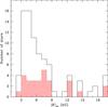 |
Fig. 1 Histogram showing the distribution of the phase-averaged mean magnetic field moduli of the 84 Ap stars with resolved magnetically split lines presently known. The shaded part of the histogram corresponds to those stars whose field modulus has been measured throughout their rotation cycle (see text). |
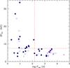 |
Fig. 2 Observed average of the mean magnetic field modulus against rotation period. Dots: stars with known rotation periods; triangles: stars for which only the lower limit of the period is known. Open symbols are used to distinguish those stars for which existing measurements do not cover the whole rotation cycle. The horizontal and vertical dashed lines, corresponding to ⟨ B ⟩ av = 7.5 kG and Prot = 150 d, respectively, emphasise the absence of very strong magnetic fields in the stars with the slowest rotation (see text for details). |
More observations should also be obtained to refine the characterisation of the low end of the ⟨ B ⟩ av distribution, so as to provide a firm basis for its theoretical understanding. In particular, we do not know at present if the bimodal character of the field strength distribution is restricted to slowly rotating stars, or if it is general feature of the magnetism of Ap stars, independent of their rotation. On the other hand, the cut-off that Aurière et al. (2007) inferred from a systematic search for weak longitudinal fields in Ap stars could represent the ultimate lower limit of the field strength distribution. However, at the low dipole strength (≲300 G) at which the ⟨ Bz ⟩ cut-off is found, measuring the mean magnetic field modulus represents a major challenge.
On the strong field side, while compared to Paper I, a few additional stars have populated the high end of the distribution of ⟨ B ⟩ av, their meaning for the characterisation of this distribution is limited, since several were observed at high resolution as the result of the detection of their exceptionally strong longitudinal fields as part of spectropolarimetric surveys. In other words, they are not a priori representative of the distribution of magnetic field strengths that one would derive from the study of an unbiased sample of Ap stars with low v sini.
In Fig. 2, we plotted ⟨ B ⟩ av against the rotation period Prot for those stars from Tables 1 and 2 for which the latter, or at least a lower limit of it, could be determined. This figure, which is an updated version of Fig. 50 of Paper I, fully confirms the result inferred from the latter, that very strong magnetic fields (⟨ B ⟩ av ≳ 7.5 kG) are found only in stars with rotation periods shorter than ~150 days. This result is visually emphasised in the figure by dashed lines: the horizontal line corresponds to ⟨ B ⟩ av = 7.5 kG, and the vertical line to Prot = 150 d. The representative points of 50 stars appear in Fig. 2. Twenty-seven of them correspond to stars with Prot < 150 d, of which 17 have ⟨ B ⟩ av ≥ 7.5 kG. By contrast, none of the 23 stars with Prot > 150 d have ⟨ B ⟩ av ≥ 7.5 kG. The difference between the two groups is highly significant: a Kolmogorov-Smirnov test indicates that the distributions of ⟨ B ⟩ av between the stars with a rotation period shorter than 150 days and those with a longer rotation period are different at the 100.0% confidence level.
This result receives further support from consideration of the stars with magnetically resolved lines whose period is unknown and for which the average of the mean magnetic field modulus over this period may exceed ~7.5 kG. Among the stars of Tables 13 and 14, this is almost certainly the case for HD 47103, HD 55540, HD 66318, HD 70702, BD +0 4535, and HD 168767. The spectral lines of HD 70702 and HD 168767 show considerable rotational broadening, so that their periods must be of the order of a few days (Elkin et al. 2012), while Elkin et al. (2010a) infer from their estimate of v sini for BD +0 4535 that its period must be shorter than ~60 days. The mean field modulus of HD 55540 shows a variation of ~600 G between two observations taken one month apart (Freyhammer et al. 2008); its period should probably be of the order of months. The situation is less clear for HD 47103 (Appendix A.8) and HD 66318 (Bagnulo et al. 2003). Both of these stars have a low v sini and neither shows definite variations of the magnetic field; either one of the angles i or β is small for these two stars or their periods are longer than one year. Obtaining more and better observations to establish if HD 47103 and HD 66318 are actually variable, and if so, to determine their periods, would represent a further test of the existence and nature of a difference in the distribution of the field strengths below and above Prot = 150 d.
There are several other stars in Table 14 for which ⟨ B ⟩ av, as computed from the few available measurements, is of the order of or slightly greater than 7.5 kG. It would be interesting to determine their periods (if they are not already known) and to obtain more ⟨ B ⟩ av measurements distributed well throughout their rotation cycle, but it appears highly improbable that any of these stars could represent a significant exception to the conclusion that very strong fields do not occur in very long-period stars.
For two of the stars that appear to rotate extremely slowly, HD 55719 and HD 165474, the scatter of the individual ⟨ B ⟩ values around a smooth, long-term variation trend is much greater than we would expect from the appearance of the Fe iiλ 6149.2 diagnostic line in their spectrum. This is unique: for all the other stars studied here, the scatter of the individual measurements of the mean field modulus about its variation curve or trend is consistent with the observed resolution of the Fe iiλ 6149.2 line, the definition of its components, and the amount of blending to which they are subject. By contrast, the radial velocity measurements for HD 55719 and HD 165474, do not show any anomalous scatter about the corresponding variation curves. On the contrary, as stressed in Sect. A.32, the exquisite precision of the radial velocity measurements in HD 165474 enabled us to detect minute long-term variations. Since those radial velocity values are computed from the very measurements of the split components of the Fe iiλ 6149.2 line from which the ⟨ B ⟩ values are obtained (see 3.3 and Eq. (15)), their high quality suggests that the unexpectedly high scatter of the mean field modulus values does not result from measurement errors nor does it have an instrumental origin. The remaining interpretation, that the observed scatter has a stellar origin, is intriguing, as it calls for additional variability on timescales considerably shorter than the rotation periods of the Ap stars of interest. This might possibly represent a new, previously unobserved type of variability for an Ap star, or those variations could originate from an unresolved companion. The data available at present are inconclusive, but this is an issue that will definitely deserve further follow up in the future.
To characterise the variability of the mean magnetic field modulus, we use the ratio q between its extrema. This ratio is given in the fifth column of Tables 13 and 14. For those stars for which we fitted a curve to the measurements (that is, the stars appearing in Tables 8 and 15), the adopted value of q is the ratio between the maximum and minimum of the fitted curve. For the other stars, the adopted value of q is the ratio of the highest to the lowest value of ⟨ B ⟩ that we measured until now (for those stars that we studied) or that we found in the literature.
The distribution of the values of q is shown in Fig. 3 for the 66 stars for which more than one ⟨ B ⟩ measurement has been obtained. In 41 of these stars, q does not exceed 1.10. This shows that the amplitude of variation of the mean magnetic field modulus is in most cases small compared to its value and supports the view that the field modulus is very useful to characterise the magnetic fields of Ap stars in statistical studies. The fact that for about two-thirds of the stars with q ≤ 1.10, the existing data do not sample (yet) the whole rotation cycle does not seriously question this conclusion, if one considers that also in ~50% of the stars for which good phase coverage is achieved (shaded part of the histogram), q does not exceed 1.10. However, for about one-fifth of the known Ap stars with magnetically resolved lines (and one quarter of those that have been observed throughout their rotation period), q is greater than 1.25, which is the upper limit for a centred dipole (Preston 1969b). This points to the occurrence of significant departures from this simple field geometry. The highest value of q obtained so far in our study is 1.95, in the star HD 65339. More recent observations by Ryabchikova et al. (2004b) suggest a similar, or even higher value of this ratio in HD 29578.
On the other hand, one can find in Fig. 4 some hint that high relative amplitudes of variation of ⟨ B ⟩ are found more frequently in stars with very long periods. In order to help the eye visualise this, two dashed lines were drawn in Fig. 4: the first is horizontal, at q = 1.3 and the second is vertical at log Prot = 2.0. Among the 21 stars with Prot < 100 d, only 2 have q > 1.3. By contrast, 8 of the 25 stars with Prot > 100 d have q > 1.3. The evidence is less compelling than for the above-mentioned absence of very strong fields in very slowly rotating stars, but the high rate of occurrence of large relative amplitudes of ⟨ B ⟩ variations among the latter nevertheless seems significant, especially if one considers that for the stars that have not been observed yet throughout a whole rotation cycle, the values of q adopted here are lower limits. In particular, among the stars with q < 1.3, phase coverage is incomplete for 10 of 17 with Prot > 100 d, but only for 4 of 19 with Prot < 100 d: thus there is significantly more possibility for future studies to increase the fraction of stars with high values of the ratio q among the long-period members of this sample than among their short-period counterparts. The proximity of the q = 1.3 dividing line to the upper limit of q for a centred dipole may further suggest that there exists a real difference in the structure of the magnetic fields below and above Prot = 100 d. The q = 1.25 value of this upper limit is only approximate; in particular, it may vary slightly according to the applicable limb-darkening law (Preston 1969b).
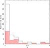 |
Fig. 3 Distribution of the ratio q between the observed extrema of mean magnetic field moduli of the 66 Ap stars with resolved magnetically split lines presently known for which more than one measurement of ⟨ B ⟩ is available. Although HD 96237 was observed twice by Freyhammer et al. (2008), its spectral lines were not resolved in the first epoch spectrum. The shaded part of the histogram corresponds to those stars that have been observed throughout their rotation cycle (see text). |
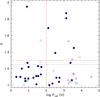 |
Fig. 4 Ratio q of the observed extrema of the mean magnetic field modulus against rotation period. Dots: stars with known rotation periods; triangles: stars for which only the lower limit of the period is known. Open symbols are used to distinguish those stars for which existing measurements do not cover the whole rotation cycle. The horizontal and vertical dashed (red) lines, corresponding to q = 1.3 and Prot = 100 d, respectively, emphasise the tendency for higher values of q to have a higher rate of occurrence in the stars with the slowest rotation. The horizontal dotted (blue) line corresponds to the upper limit of q for a centred dipole (see text). |
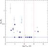 |
Fig. 5 Ratio M2/M1 of the fit coefficients given in Tables 8 and 15 against rotation period. Open circles: stars showing ⟨ Bz ⟩ reversal; dots: stars in which ⟨ Bz ⟩ has a constant sign; open triangle: star for which no ⟨ Bz ⟩ measurements exist. For a fraction of the stars, the error bar is shorter than the size of the representative symbol. The horizontal (solid) line corresponds to the stars for which the curve of variation of ⟨ Bz ⟩ does not significantly depart from a sinusoid (M2 = 0). The two vertical (dashed) lines emphasise the tendency for anharmonicity of the mean field modulus variations to be restricted to rotation periods shorter than Prot = 100 d or greater than Prot = 1000 d. |
In order to explore the dependency on rotation period not only of the amplitude of the curve of variation of the field modulus, but also of its shape, in Fig. 5 we plotted against the rotation period, the ratio M2/M1 of the amplitude of the harmonic to that of the fundamental in a fit of the ⟨ B ⟩ data by a function of the form given in Eq. (17). Zero values of this ratio correspond to the cases where the measurements are adequately represented by a single sinusoid (Eq. (16)). The pattern that appears in Fig. 5 is intriguing. The curves of variation of ⟨ B ⟩ show a significant degree of anharmonicity for the majority of the stars with Prot < 100 d (but not for all of them). For rotation periods between 100 and 1000 days, the variation curves are mostly sinusoidal. For three of the four stars with Prot > 1000 d for which we accumulated enough data to fully define the shape of the ⟨ B ⟩ variation curve, a significant first harmonic is present in the fits. Furthermore, there are at least three more stars whose rotation periods exceed 1000 days and for which the data acquired so far are insufficient to characterise the variation curve of the mean field modulus completely, for which this curve is definitely anharmonic:
-
The variation curve of the field modulus ofHD 965, which has a rotation period considerablylonger than 10 yr, shows a very broad, almost flatminimum (Elkin et al. 2005a).
-
The ⟨ B ⟩ variations in HD 9996, which has a rotation period of ~22 yr, must have a high degree of anharmonicity, according to the arguments given in Appendix A.3.
-
The ⟨ B ⟩ variations in HD 166473, whose rotation period may be of the order of 10 yr, also show definite anharmonicity (Mathys et al. 2007).
The interpretation of the behaviour pattern that is observed in Fig. 5 is not straightforward at this stage. We postpone its discussion to Sect. 5.2.
On the other hand, among the fitted ⟨ B ⟩ curves, 7 show two (generally different) minima and two (generally different) maxima per rotation period. We introduce the notations ⟨ B ⟩ max,1 and ⟨ B ⟩ max,2 to refer to, respectively, the primary (greater) and secondary maxima, and ⟨ B ⟩ min,1 and ⟨ B ⟩ min,2 for the primary (smaller) and secondary minima. Interestingly, in all but one of the stars for which these quantities are defined, the difference ⟨ B ⟩ max,1− ⟨ B ⟩ max,2 between the primary and secondary maxima of the field modulus is significantly larger than the difference between its secondary and primary minima, ⟨ B ⟩ min,2− ⟨ B ⟩ min,1. This must be related to the observation in a number of stars of broad, more or less flat minima of the ⟨ B ⟩ variation curve, mentioned on several occasions in Appendix A. In other words, it is rather usual for the mean magnetic field modulus to be close to its minimum value over a large portion of the rotation period, and to show a rather steep variation from near minimum to an absolute maximum and back within a fairly narrow phase range. The common character of this behaviour is further supported by consideration of other stars, whose ⟨ B ⟩ curves have only one minimum and one maximum per cycle, but show shallower variations about their phase of minimum than around their maximum: HD 59435, probably HD 166473 (if its rotation period is close to 10 yr), and HD 192678. HD 965 is another star that almost certainly shows a similar behaviour. By contrast, we did not observe any star showing a broad, shallow maximum of the field modulus and a narrower, steeper minimum. Also, for the only star found so far in which (⟨ B ⟩ max,1− ⟨ B ⟩ max,2) < ( ⟨ B ⟩ min,2− ⟨ B ⟩ min,1), HD 200311, the difference between the two sides of the inequality is more moderate than in most stars in which (⟨ B ⟩ max,1− ⟨ B ⟩ max,2) > ( ⟨ B ⟩ min,2− ⟨ B ⟩ min,1). Actually, owing to the incomplete phase coverage of the field modulus determinations for this star, it is not implausible that the value of (⟨ B ⟩ min,2− ⟨ B ⟩ min,1) derived from our observations overestimates the actual field strength difference between the two minima (see Fig. A.68).
Magnetic parameters of Ap stars with resolved magnetically split lines: stars with ⟨ B ⟩ data from the literature.
Variation of the mean magnetic field modulus: least-squares fit parameters for data from the literature.
Regardless, we have not observed any star in which the difference between the minima of the field modulus is much greater than the difference between its maxima. This probably indicates that it is frequent for Ap stars to have a fairly uniform magnetic field (such as a global dipole) covering the largest part of their surface, with one rather limited region (a kind of large spot) where the field is much stronger. In this spot the small-scale structure of the field must be considerably more complex than in the rest of the star, since its signature is not readily seen in the longitudinal field variations (see Sect. 5.2). The opposite topology, a star with a large spot that has a lower field than the surroundings, does not seem to occur commonly, if at all. If this interpretation is indeed correct, it suggests that models based on low-order multipole expansions are unlikely to provide a very good representation of the actual field geometries, even though they may provide useful first order approximations.
The frequent occurrence in the ⟨ B ⟩ variation curves of nearly flat minima extending over a broad phase range implies that the probability of observing a star when its field modulus is close to its minimum value is, in general, significantly higher than close to its maximum value. This, in turn, means that for those stars for which we have observed so far a constant, or nearly constant value of ⟨ B ⟩, this value is likely to correspond roughly to the minimum of this field moment. It can be expected that, if the star varies at all, at some point it will start to show a comparatively steep increase towards higher values of the field modulus; by contrast, it seems improbable that ⟨ B ⟩ starts to decrease after it remained nearly constant for an extended period of time.
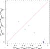 |
Fig. 6 Difference between the primary and secondary maxima of the mean magnetic field modulus against the difference between its two minima; both differences are normalised via division by the difference between the primary maximum and primary minimum. Open circles represent stars whose longitudinal field reverses its sign over a rotation period; the dot corresponds to a star with non-reversing longitudinal field. The dashed line is drawn to help the eye visualise the fact that the difference between the minima is generally smaller, and never much greater than the difference between the maxima. The only star above this line is HD 200311, for which no ⟨ B ⟩ data could be obtained between phases 0.6 and 0.9. More observations of the star in this phase range might possibly shift its representative point below the dashed line. |
Another intriguing result is shown in Fig. 6, where the difference between the primary and secondary minima of the mean magnetic field modulus is plotted against the difference between its two maxima, for those stars where ⟨ B ⟩ has two maxima and two minima per period. Both differences are normalised via division by the difference between the primary maximum and primary minimum, so as to allow for comparison between stars with different field strengths. The dashed diagonal line, which corresponds to ⟨ B ⟩ min,2− ⟨ B ⟩ min,1 = ⟨ B ⟩ max,1− ⟨ B ⟩ max,2, is shown for easier visualisation of the above-mentioned result, that the difference between the ⟨ B ⟩ minima is in general smaller, and never much greater, than the difference between its maxima. Very unexpectedly, a rather tight anti-correlation appears, namely, 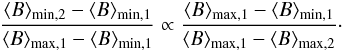 In other words, for a given peak-to-peak amplitude of variation of the field modulus, the greater the difference between the two minima is, the smaller the difference between the two maxima. We know of no obvious reason why this should be so; as a matter of fact, if the field were a centred dipole (which is not an implausible geometry), both differences would be zero. Thus the observed behaviour provides a constraint on the systematics of the field structure of magnetic Ap stars. Admittedly, this result is deduced from consideration of only seven stars, so that its statistical significance is still moderate, but the observed anti-correlation is very obvious.
5.2. The mean longitudinal magnetic field
We have presented 231 new measurements of the mean longitudinal magnetic field of 34 Ap stars with resolved magnetically split lines. For 10 of these stars, these are the first determinations of this field moment ever published.
The ⟨ Bz ⟩ measurements reported here are the most precise ever obtained with the CASPEC spectrograph. This is best seen by comparing the median of the standard errors σz of all the measurements appearing in Table 6, 98 G, with their median for the 44 measurements of ⟨ Bz ⟩ in Ap stars with magnetically resolved lines previously published by Mathys (1994) and Mathys & Hubrig (1997), 159 G. Such a comparison is more meaningful than a comparison with all the previous ⟨ Bz ⟩ determinations based on CASPEC observations, since errors increase quickly with v sini. The better precision of the present data results from the combination of several factors: (1) The spectra were obtained at a resolving power R ~ 3.9 × 10⁴, which is more than twice as high as that used by Mathys (1994) and for a fraction of the observations of Mathys & Hubrig (1997), R ~ 1.6 × 10⁴. (2) Their spectral coverage, continuous over a range of the order of 1250 Å, is at least comparable to that of the lower resolution spectra of the above-mentioned papers, and much larger than that (~600 Å, once the inter-order gaps have been subtracted) of the higher resolution (R ~ 3.5 × 10⁴) spectra of Mathys & Hubrig (1997). (3) The combination of a new Zeeman analyser (used by Mathys & Hubrig for only a few of their observations), a CCD with higher sensitivity, and improvements in the optical alignment of CASPEC and in its stability, enabled us to achieve a considerably higher signal-to-noise ratio in the reduced spectra.
The precision of the present ⟨ Bz ⟩ measurements compares well with that of the contemporaneous determinations of Wade et al. (2000b), which were achieved through application of the least-squares deconvolution (LSD) technique to spectra recorded with the spectrograph MuSiCoS. The median standard error of the MuSiCoS measurements is 48 G. This is a factor of 2 smaller than what we achieve here, which can be accounted for by the fact that the spectral coverage of MuSiCoS is about four times larger than that of CASPEC in the configuration that we used. Admittedly, the comparison is valid only for the low values of v sini typical of our sample; for stars with higher projected equatorial velocities, the LSD technique is more robust, in particular against line blending.
Because the mean longitudinal magnetic field is very sensitive to the geometry of the observation, so that, in particular, it may reverse its sign as the star rotates, the average of all the obtained measurements of ⟨ Bz ⟩, or the independent term Z0 of the fit of their variation curves, is inadequate to characterise this field moment in a given star by a single number, as we did for the mean magnetic field modulus. To this effect, following Bohlender et al. (1993), we use instead the root-mean-square (rms) longitudinal field, defined as 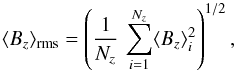 (18)where Nz is the number of individual measurements of ⟨ Bz ⟩ that we obtained, and ⟨ Bz ⟩ i is the i-th such measurement. The values of Nz and ⟨ Bz ⟩ rms are given in Cols. 6 and 7 of Tables 13 and 14. For most stars of Table 13, as in the rest of this paper, these values were computed by combining the new ⟨ Bz ⟩ determinations presented here with the published CASPEC-based values of Mathys (1994) and Mathys & Hubrig (1997). For a few northern stars, which could not be observed with CASPEC and for which recent, reliable measurements of the longitudinal field distributed well throughout the rotation cycle are available in the literature, the values of Nz and ⟨ Bz ⟩ rms appearing in Table 13 (in italics) were computed using these published data: HD 9996 (Bychkov et al. 2012), HD 12288 and HD 14437 (Wade et al. 2000c), HD 18078 (Mathys et al. 2016), HD 65339 (Wade et al. 2000b; Bagnulo et al. 2001), HD 192678 (Wade et al. 1996a), and HD 200311 (Wade et al. 1997; Leone et al. 2000). Finally, the Nz and ⟨ Bz ⟩ rms data of Table 14 are based on the ⟨ Bz ⟩ measurements from the references listed in Col. 8 of that table.
The distribution of the values of ⟨ Bz ⟩ rms for Ap stars with resolved magnetically split lines, shown in Fig. 7, differs markedly from their distribution for all Ap stars (see Fig. 1 of Bychkov et al. 2003). The deficiency of stars with ⟨ Bz ⟩ rms< 0.5 kG among the stars of the present sample starkly contrasts with the fact that 50% of all Ap stars have ⟨ Bz ⟩ rms< 525 G (see Table 1 of Bychkov et al. 2003). This difference is further emphasised if one focuses attention on the stars for which longitudinal field measurements were obtained throughout the full rotation cycle (i.e. the shaded part of the histogram in Fig. 7). One can reasonably expect that, as more data are obtained for the stars for which phase coverage is so far incomplete, the shape of the unshaded part of the histogram progressively becomes more similar to the shaded part, at least up to 2 kG, so that the lack of low ⟨ Bz ⟩ rms values stands out even more conspicuously. This scarcity of weak longitudinal fields in our sample is not unexpected, since magnetic fields that are strong enough to produce line splitting sufficiently large to be resolved observationally should, in their majority, also have a sizeable mean longitudinal component. However, as we show below, there is no one-to-one relation between ⟨ Bz ⟩ rms and ⟨ B ⟩ av.
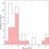 |
Fig. 7 Histogram showing the distribution of the root-mean-square longitudinal magnetic field of the 49 Ap stars with resolved magnetically split lines for which this field moment was measured at least once. The shaded part of the histogram corresponds to those stars whose longitudinal field has been measured throughout their rotation cycle (see text). |
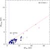 |
Fig. 8 Observed root-mean-square longitudinal field against the observed average of the mean magnetic field modulus. Open symbols are used to distinguish those stars for which either or both of ⟨ Bz ⟩ rms and ⟨ B ⟩ av were computed using less than 7 individual measurements of, resp., ⟨ Bz ⟩ and ⟨ B ⟩; triangles are used for field modulus values from the literature. The dashed line corresponds to ⟨ Bz ⟩ rms = ⟨ B ⟩ av/ 3. For only two stars (identified in the figure), the representative points are clearly above this line. However this is significant only for HD 215441, since the number of measurements of HD 157751 is insufficient (see text). The dotted vertical line corresponds to ⟨ B ⟩ av = 2.8 kG; it emphasises the discontinuity at the low end of the distribution of ⟨ B ⟩ av, discussed in Sect. 5.1. |
Variation of the mean longitudinal magnetic field: least-squares fit parameters for data from the literature.
In Fig. 8, we plotted ⟨ Bz ⟩ rms against ⟨ B ⟩ av. One can see that only two points are found significantly above a (dashed) line corresponding to ⟨ Bz ⟩ rms = ⟨ B ⟩ av/ 3. Although the slope that we adopted for this line is purely empirical, based only on the observational points, it is interesting to note the following similarity. As shown by Preston (1970), for a centred dipole, the maximum of the ratio between the absolute value of ⟨ Bz ⟩ and ⟨ B ⟩, (| ⟨ Bz ⟩ | / ⟨ B ⟩ )max, can be at most of the order of 0.4; this value is reached only when the dipole axis becomes parallel to the line of sight at some rotation phase. This phase also corresponds to an extremum of ⟨ Bz ⟩. Since the amplitude of the variations of ⟨ B ⟩ is typically small, in first approximation (| ⟨ Bz ⟩ | / ⟨ B ⟩ )max ~ | ⟨ Bz ⟩ | max/ ⟨ B ⟩ av, where | ⟨ Bz ⟩ | max is the maximum of the absolute value of ⟨ Bz ⟩. On the other hand, ⟨ Bz ⟩ rms is always smaller than (or equal to) | ⟨ Bz ⟩ | max. In particular, for a star in which ⟨ Bz ⟩ shows sinusoidal variations with an amplitude much greater than the absolute value of its mean (Z1 ≫ | Z0 |), ⟨ Bz ⟩ rms is of the order of  . Thus, for a centred dipole, one would expect the ratio ⟨ Bz ⟩ rms/ ⟨ B ⟩ av not to be significantly greater than
  . The similarity between this number and the value 1/3 represented by the dashed line in Fig. 8 suggests that, even though actual field structures often show significant departures from a centred dipole (as indicated in particular by other arguments presented elsewhere in this paper), the latter represents a good first approximation in most cases.
Babcock’s star, HD 215441, represents a remarkable exception to this general conclusion. Its location in Fig. 8, well above the ⟨ Bz ⟩ rms = ⟨ B ⟩ av/ 3 line, distinguishes it very clearly from the bulk of the considered sample, and emphasises its exceptional character. Not only has it stood for more than 50 yr as the star with the strongest known mean magnetic field modulus since its discovery by Babcock (1960), but also the structure of its magnetic field now appears to be very different from that of almost all other magnetic Ap stars. HD 215441 definitely cannot be considered a representative member of the class. Whether the outstanding structure of its magnetic field is related to the unusual field strength, or whether the conjunction of these two features is the result of a mere coincidence cannot be definitely established on the basis of the existing observational evidence. One may note, however, that in HD 75049, which among the Ap stars with magnetically resolved lines has the second highest value of ⟨ B ⟩ av, ⟨ Bz ⟩ rms/ ⟨ B ⟩ av = 0.25. Moreover, it also appears highly unlikely that this ratio may significantly exceed 1/3 in HD 154708 (which has the third highest value of ⟨ B ⟩ av), even though the variations of its mean field modulus are not fully characterised. These considerations support the view that Babacock’s star has an extremely unusual magnetic field structure.
For the other star whose representative point in Fig. 8 lies significantly above the ⟨ Bz ⟩ rms = ⟨ B ⟩ av/ 3 line, HD 157751, this departure from the general trend most likely is purely circumstantial since the values of ⟨ Bz ⟩ rms and ⟨ B ⟩ av are based on only 2 and 1 measurements, respectively. As such, these values cannot be expected (especially the former) to represent accurate estimates of the actual values of the considered quantities, which are meant to be averages over the stellar rotation period.
On the other hand, the discontinuity at 2.8 kG at the low end of the distribution of the values of ⟨ B ⟩ av is clearly seen in Fig. 8, where it is emphasised by a dotted line parallel to the ordinate axis. No similar discontinuity is apparent in the distribution of ⟨ Bz ⟩ rms (but see Aurière et al. 2007).
For 17 stars, the phase sampling of our spectropolarimetric observations lends itself to carrying out a quantitative characterisation of the shape of the variation curve of the longitudinal field by fitting the ⟨ Bz ⟩ measurements by a function of the form given in Eqs. (16) or (17). The fit parameters are given in Table 9. In the case of HD 2453, HD 137949, and HD 188041, they were derived by combining our ⟨ Bz ⟩ data with measurements from the literature: see Appendices A.2, A.27, and A.36 for details. Furthermore, the curves of variation of the longitudinal field of the 6 northern stars HD 9996, HD 12288, HD 14437, HD 18078, HD 65339, and HD 200311 are well constrained by the data of the references cited above. The seventh northern star of our study that could not be observed with CASPEC but for which a good recent set of ⟨ Bz ⟩ measurements exists in the literature, HD 192678, does not show variations of this field moment above the noise level, so that no significant fit can be computed. This star should be regarded as having a constant longitudinal field at the achieved precision. On the other hand, an additional 4 stars from Table 14, which were not part of our observing sample, also have well defined ⟨ Bz ⟩ variation curves; these are HD 75049 (Kochukhov et al. 2015), HD 154708 (Bagnulo et al. 2015), HD 178892 (Ryabchikova et al. 2006), and HD 215441 (Borra & Landstreet 1978). The fit parameters computed from the published measurements of the longitudinal field of the 10 stars identified above are presented in Table 16. Its format is identical to that of Table 9. The phase origins and the period values used for these fits are listed in Tables 1 and 2.
Thus, in total, there are now 28 stars with magnetically resolved lines for which the variations of ⟨ Bz ⟩ with rotation phase are characterised, against 10 at the time of publication of Paper I.
Anharmonicity in the ⟨ Bz ⟩ variation curves occurs less frequently and is in general less pronounced than in the ⟨ B ⟩ variation curves. The fraction of Ap stars with magnetically resolved lines in which a fit of the observations by a cosine curve and its first harmonic is found to be better than a fit by a single cosine is not significantly different from this fraction in the samples of Ap stars considered in previous CASPEC studies (Mathys 1994; Mathys & Hubrig 1997). In other words, on the basis of this (admittedly limited) comparison, there is no evidence of a relation between the anharmonicity of the ⟨ Bz ⟩ variations of Ap stars and the length of their rotation period. The comparison with longitudinal field determinations obtained by other authors is not meaningful since systematic differences are frequent between ⟨ Bz ⟩ measurements obtained with different instruments and/or methods.
The relative amplitude of variation of the longitudinal field is customarily characterised by the parameter r = ⟨ Bz ⟩ s/ ⟨ Bz ⟩ g, where ⟨ Bz ⟩ s is the smaller and ⟨ Bz ⟩ g the greater (in absolute value) of the observed extrema ⟨ Bz ⟩ max and ⟨ Bz ⟩ min of ⟨ Bz ⟩ (see Paper I, for details about the physical meaning of r).
The ratio q = ⟨ B ⟩ max/ ⟨ B ⟩ min of the extrema of ⟨ B ⟩ is plotted against r in Fig. 9. The values of r and q correspond to the extrema of the fitted curves of the variation of the ⟨ Bz ⟩ and ⟨ B ⟩ measurements, respectively, using the fit parameters of Tables 8, 9, 15, and 16. There are 22 stars for which both fits appear in these tables. In addition, we consider the field modulus as constant in HD 116458, for which a fit to the ⟨ Bz ⟩ variation curve is available; and conversely in HD 192678, the ⟨ B ⟩ variation curve is well defined while ⟨ Bz ⟩ is not significantly variable.
Figure 9 is an updated version of Fig. 53 of Paper I. With respect to this Paper I figure, the number of stars for which the relevant information is available has doubled. Consideration of this sample of increased statistical significance strengthens the result found in Paper I that the representative points of all the stars are concentrated towards the lower left half of the figure. This is emphasised by the dashed line crossing the figure in diagonal. The star most significantly above this line, HD 65339 (identified in the figure), is also the star with the highest value of q confirmed so far. However, its location in Fig. 9 remains rather close to the area where the majority of the studied stars are concentrated. The conclusion that a significant difference generally exists between the two poles of the studied stars, which was drawn in Paper I from consideration of the distribution of the representative points in the q versus r diagram, is strengthened.
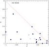 |
Fig. 9 Relative amplitude q of the variation of the mean magnetic field modulus against the ratio r of the extrema of the mean longitudinal field (see text). Dots identify values of q computed from the ⟨ B ⟩ data of this paper and of Paper I; triangles are used for field moduli from the literature. Filled symbols correspond to stars for which the ⟨ Bz ⟩ measurements are based on CASPEC observations (this paper; Mathys 1994; Mathys & Hubrig 1997), open symbols to other good ⟨ Bz ⟩ measurements from the literature (references given in the text). The dashed diagonal line, q = (3−r)/2, emphasises the concentration of the majority of the stars of the sample in the lower left part of the figure: namely, high amplitudes of variation of ⟨ B ⟩ are observed when both the positive and negative magnetic poles of the star come into sight during its rotation cycle. |
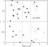 |
Fig. 10 Ratio r of the extrema of the mean longitudinal magnetic field (see text) against rotation period. Dots: stars with known rotation periods; triangles: stars for which only the lower limit of the period is known. Open symbols are used to distinguish those stars for which existing measurements do not cover the whole rotation cycle. Stars with representative points below the long-dashed horizontal line have reversing mean longitudinal fields. The two vertical (dashed) lines emphasise the tendency for longitudinal fields showing sign reversals to be restricted to rotation periods shorter than Prot = 100 d or longer than Prot = 1000 d. |
Not surprisingly, very long rotation periods are under-represented in Fig. 9, compared to the whole group of known stars with resolved magnetically split lines. As a matter of fact, only three stars with rotation periods longer than 1000 d have representative points; these are HD 18078, HD 94660, and HD 187474. If we assume that the rotation period of HD 166473 is close to the time span over which its mean magnetic field modulus has been studied so far, we can use the same tentative value of the period as Landstreet & Mathys (2000; Prot = 4400 d) to obtain good fits of the variation curves of ⟨ Bz ⟩ and ⟨ B ⟩ (including all measurements of Table 1 of Mathys et al. 2007) with functions of the form given in Eq. (17). From these fits, we derive r = −0.84 and q = 1.50. These values should represent good approximations of the actual values of the r and q parameters for this star, as long as its rotation period is not much longer than 12 yr. The corresponding location of the representative point of the star in Fig. 9 would be below the q = (3−r)/2 line, consistent with the rest of the studied sample. For HD 9996 (Prot ~ 22 yr), an exact value of r = −0.35 is derived from the fully constrained curve of variation of ⟨ Bz ⟩, but only a lower limit can be set for q (q> 1.34) since measurements of ⟨ B ⟩ have been obtained only over a fraction of the rotation period. This is compatible with the location of the representative point of the star below the q = (3−r)/2 line, but it is not impossible that the actual ratio of the extrema of the field modulus may be greater than the maximum predicted from this line, q = 1.675. This would only require ⟨ B ⟩ to become of the order of 3 kG or smaller over part of the rotation cycle, which is not implausible at all since the Fe iiλ 6149.2 line is definitely not resolved at some phases. Thus the representative point of HD 9996 in Fig. 9 may well be above the line drawn through it, which would represent another exception to the tendency of the majority of the stars to concentrate in the lower left part of the q versus r diagram. This is not entirely surprising, since it was already apparent from the shapes of the spectral lines that the magnetic field of HD 9996 must have a rather unusual structure (see Appendix A.3).
Figure 10 illustrates the behaviour of r as a function of the stellar rotation period. Besides the 27 stars listed in Tables 9 and 16 for which the longitudinal field variations were quantified by fits of the forms given in Eqs. (16) or (17), this figure includes representative points of
-
1.
HD 192678, for which ⟨ Bz ⟩ does not show any significant variation.
-
2.
HD 166473, for which we assumed that Prot = 4400 d and r = −0.84 are suitable, although inexact, representative values (see above).
-
3.
HD 335238, whose period is reliably determined but only sampled in a very incomplete manner by the existing ⟨ Bz ⟩ measurements.
-
4.
Seven stars for which only a lower limit of the period has been established so far. For all of these stars, this lower limit exceeds 1000 days; it is used as the abscissa of their representative point in Fig. 10.
For the stars identified under items 3 and 4 above, we computed r adopting for ⟨ Bz ⟩ min and ⟨ Bz ⟩ max the observed extreme values of the longitudinal field. Given the nature of the variations of this field moment, these observed extreme values may greatly differ from the actual extrema of variation of ⟨ Bz ⟩; they may even have a different sign. Thus the preliminary values of r derived here for those stars for which the available ⟨ Bz ⟩ data cover only a fraction of the variation curve can also be strongly different from their actual values. However, if the preliminary value of r obtained here is negative, its actual value, based on the full variation curve of the longitudinal field of the star, must definitely be negative as well. By contrast, a positive preliminary value of r does not constrain its final sign, since the possibility of a sign reversal of ⟨ Bz ⟩ at a phase not yet observed remains open. In particular, HD 29578, whose representative point is labelled, appears in the figure with r > 0 only because of the incomplete phase coverage of the available longitudinal field measurements. But its incomplete ⟨ Bz ⟩ variation curve (Fig. A.12) indicates unambiguously that the mean longitudinal field must reverse its sign in that star, so that it actually has r < 0. On the other hand, the mean longitudinal field of HD 335238, which is represented in Fig. 10 by an open circle, also definitely reverses its sign, but not enough measurements have been obtained to characterise its variations fully over the well-established rotation period.
Two short-dashed, vertical lines in Fig. 10 at Prot = 100 d and Prot = 1000 d emphasise the following apparent correlation. All but one of the 7 stars with a period in the range [100...1000] d have a non-reversing mean longitudinal field (r > 0). By contrast, r < 0 for 6 of the 17 stars with Prot < 100 d and for 8 of the 12 stars with Prot > 1000 d (taking into account the remark above about HD 29578). For rotation periods exceeding 100 days, the stellar equatorial velocity v is low enough so that the observation of resolved magnetically split lines does not set any constraint on the inclination angle i of the rotation angle to the line of sight. Thus one should expect the distribution of the values of i to be random: any difference in the distribution of the values of r between the period ranges 100 ≤ Prot ≤ 1000 d and Prot > 1000 d must reflect a difference in the distribution of the values of the angle β between the magnetic and rotation axes. The behaviour of r illustrated in Fig. 10 suggests that the rate of occurrence of large values of β is higher for rotation periods longer than 1000 days than for periods between 100 and 1000 days. On the other hand, for the stars with the shortest rotation periods of the sample (say, Prot< 30 d), i must be small enough so that Doppler broadening does not smear out the magnetic splitting of the spectral lines. Thus again the difference in the rate of occurrence of negative values of r suggests that β must in general be greater for stars with rotation periods shorter than 30 days than for stars with rotation periods between 100 and 1000 days.
Admittedly, the moderate size of the sample limits the statistical significance of the conclusions that can be drawn from inspection of Fig. 10. Those conclusions cannot be meaningfully submitted to quantitative statistical tests. The high rate of occurrence of large values of β in stars with either the shortest periods (Prot < 100 d) or very long periods (Prot > 1000 d) seems definite, even though the best locations of the dividing lines between the three period ranges of interest may be debated. But with only 7 stars with rotation periods in the [100...1000] d range, one may legitimately wonder if the paucity of reversing mean longitudinal magnetic fields in this interval is not a mere statistical fluke. This is a possibility that cannot be easily ruled out, since the majority of the known Ap stars with 100 ≤ Prot ≤ 1000 d appear in Fig. 10. HD 221568 (Prot = 159 d) is the only other star with a well-established period in that range that is listed in the Catalano & Renson (1998) catalogue and its supplement (Renson & Catalano 2001). Among the Ap stars with resolved magnetically split lines, HD 110274 has  (see Table 2). There are not enough ⟨ Bz ⟩ data available for either of these two stars to decide whether r is positive or negative.
The pattern apparent in Fig. 10 can be related to the conclusion reached by Landstreet & Mathys (2000) that magnetic Ap stars with long rotation periods (greater than a month) have their magnetic and rotation axes nearly aligned, unlike shorter period Ap stars in which the angle between these two axes is usually large. This conclusion was reached from computation of models of the fields of the studied stars consisting of the superposition of collinear, centred, dipole, quadrupole, and octupole components. It was supported by the results of a separate study by Bagnulo et al. (2002), who assumed that the magnetic topology of the stars of interest is described by the superposition of a dipole and a quadrupole field at the centre of the star with arbitrary orientations; in this case, the angle under consideration is that between the dipole axis and the rotation axis. With respect to these earlier results, with more information now available about the longest-period stars, a new trend that had been previously unnoticed appears in Fig. 10. Namely, the tendency for the magnetic and rotation axes to be aligned seems to be restricted to an intermediate period range, while the angle between them appears to be predominantly large both in stars with relatively short periods and in stars with extremely long periods. If anything, the additional evidence presented here rather questions the robustness of the conclusion reached in earlier studies about the existence of a systematic difference in the magnetic geometries between stars with rotation periods shorter than 30–100 days and stars with periods above this value.
In light of the discussion presented in this section, the interpretation of the dependence on the rotation period of the anharmonicity of the variations of the mean magnetic field modulus, illustrated in Fig. 5, becomes clear. This can be understood by using different symbols in Fig. 5 to distinguish those stars where a sign reversal of ⟨ Bz ⟩ is observed (r < 0; open circles) from those where ⟨ Bz ⟩ is found to have always the same sign (r > 0; dots). For one star, HD 59435 (open triangle), no longitudinal field determinations were obtained.
Then, a clear-cut result appears: all but one of the stars in which the field modulus variations show no significant deviation from a sinusoid have a non-reversing longitudinal field. The exception is HD 18078, whose magnetic field appears to have a very unusual structure (see below). This implies that anharmonicity in the ⟨ B ⟩ curve generally occurs when both poles come into sight as the star rotates.
This is not surprising. For the simplest magnetic geometry, a centred dipole, if both poles come alternatively into view as the star rotates, the ⟨ B ⟩ variation curve is a perfect double wave, that is, a sinusoid with twice the rotation frequency of the star with no contribution of the fundamental. By contrast, if the angle between the rotation axis and line of sight is small, or if the angle between the magnetic and rotation axes of the star is small so that the same pole remains visible at all times, the shape of the variation of ⟨ B ⟩ is a sinusoid with the rotation period of the star. In summary, Fig. 5, as Fig. 10, suggests that the angle β between the magnetic and rotation axes is statistically large in stars with rotation periods shorter than 100 days or longer than 1000 days, while the two axes tend to be aligned in the period range [100...1000] d.
In addition, it is remarkable and highly significant that none of the mean field modulus variation curves for the stars of the studied sample are perfect double sinusoids. This strongly indicates that the two magnetic poles of (slowly rotating) Ap stars are different: the magnetic field structures significantly depart from centred dipoles. This conclusion had already been reached in Paper I; it is strengthened here because of the increase in the number of stars with fully characterised mean field modulus variations.
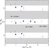 |
Fig. 11 Phase difference φZ1−φM1 (modulo 1) between the fundamentals of the fits of the measurements of ⟨ Bz ⟩ and ⟨ B ⟩ by functions of the forms given in Eqs. (16) or (17), against stellar rotation period. Open symbols: stars showing ⟨ Bz ⟩ reversal; filled symbols: stars in which ⟨ Bz ⟩ has a constant sign. Among the latter, stars with positive values of ⟨ Bz ⟩ are represented by dots, while triangles correspond to negative values of ⟨ Bz ⟩. For a fraction of the stars, the error bar is shorter than the size of the representative symbol. Shaded zones correspond to forbidden regions where representative points of stars with dipole-like fields are not expected to be found. We identified three stars that depart from this expected behaviour. |
For the first time, we built a statistically significant sample of stars for which both the curves of variation of the mean magnetic field modulus and of the mean longitudinal magnetic field are fully characterised. This gives us an unprecedented opportunity to study the relation between the variations of these two field moments. In Fig. 11, which is based on Tables 8, 9, 15, and 16, the phase lag φZ1−φM1 (modulo 1) between the fundamental components of the fits by a function of the form given by Eqs. (16) or (17) of the ⟨ Bz ⟩ measurements, on the one hand, and of the ⟨ B ⟩ data, on the other hand, is plotted against stellar rotation period. Admittedly, a significant number of the studied stars show some degree of anharmonicity in the variations of either or both of the considered field moments. But in the vast majority of these stars, the amplitude of the harmonic is considerably smaller than that of the fundamental, so that in first approximation, the actual phases of extrema do not differ much from those of the fundamental. Moreover, if (as is widely believed) the field geometry is dominated by a nearly dipolar component encompassing the whole star, on which higher order, smaller scale structures are superimposed, consideration of the fundamental in the study of phase relations between various field moments makes sense on physical grounds, since the large-scale structure to which it corresponds seems more likely to lend itself to the study of star-to-star systematics in the field properties.
For a centred dipole and for some of the most commonly used axisymmetric field models, such as a dipole offset along its axis that passes through the centre of the star (e.g. Preston 1970) or the superposition of collinear centred dipole, quadrupole, and octupole (e.g. Landstreet & Mathys 2000), one expects the fundamental components of the variations of ⟨ Bz ⟩ and ⟨ B ⟩ to be in phase or in anti-phase. For fields showing modest departures from these simple models, φZ1−φM1 should accordingly remain close to 0 or to 0.5. To reflect this expectation, in Fig. 11 we shaded the bands corresponding to 0.1 ≤ φZ1−φM1 ≤ 0.4 and 0.6 ≤ φZ1−φM1 ≤ 0.9, which should be forbidden regions for the representative points of stars with nearly dipolar fields. One can see that, consistent with the view that Ap stars have magnetic structures dominated by a dipole-like component, the vast majority of the stars of the present sample are confined to the allowed (unshaded) regions of the figure, or at least are not significantly outside them. HD 18078 and HD 137909 are clear exceptions. HD 51684 is a marginal exception, 2.6σ below the strict limit φZ1−φM1 = 0.4, which however is fairly arbitrary. These three stars are labelled in the figure.
The poor phase distribution of the existing measurements of the magnetic field of HD 51684, especially of the longitudinal field, implies that the shapes of their variations are poorly constrained, possibly to an extent worse than indicated by the formal standard errors of the fits. Accordingly, it would be tempting to regard the apparent departure of the star from normality in Fig. 11 as spurious. However, consideration of Fig. A.20 leaves little doubt about the reality of the existence of a very significant phase shift between the extrema of the longitudinal field and the field modulus. But the available observations are insufficient to lend themselves to a more detailed discussion of this unusual and interesting case.
By contrast, the curves of variation of ⟨ Bz ⟩ and ⟨ B ⟩ in HD 137909 are defined beyond any ambiguity (not only in the present study, but also in other published works; see Appendix A.26 for some recent references), and while the anharmonicity of the field modulus variations is significant, it can by no means account for the high value of φZ1−φM1. Hence the location of the representative point of HD 137909 in one of the “forbidden” regions of Fig. 11 is highly significant; it earmarks the star as extremely anomalous. This is not altogether surprising. HD 137909 has long since been one of the prototypes of the group of the Ap stars, and among its members is one that shows some of the most striking spectral and chemical peculiarities. The discrepancies between the field modulus determinations in this star obtained from AURELIE spectra and those based on other spectrographs are unique; this is the only star of the present sample in which the two groups of measurements could not be reconciled in a simple manner (e.g. by applying a constant offset). The uniqueness of the star in this respect most likely arises from the fact that the structure of its magnetic field is very different from that of most other stars. The failure by Bagnulo et al. (2000) to find a model that adequately represents the behaviour of all the magnetic moments of the star, despite using a fairly sophisticated representation of the field structure, is another sign that points to a very unusual geometry (see also Bagnulo et al. 2001).
HD 18078 has been much less studied. But the phase shift between the variation curves of its longitudinal field and its field modulus, which is as significant as for HD 137909, is not the only observable manifestation of the unusual structure of its magnetic field. This unusual structure is also revealed by the significant broadening of its resolved line components, which restricts our ability to determine its field modulus close to its phase of minimum (see Appendix A.6), and by the fact that this star is one of only a handful of stars to shown anharmonic ⟨ Bz ⟩ variations while its ⟨ B ⟩ variation curves does not significantly depart from a sinusoid.
Leaving those three exceptions aside, another remarkable feature appears in Fig. 11, when one distinguishes stars with reversing longitudinal fields (represented by open symbols) from stars with longitudinal fields keeping the same sign throughout the rotation period (filled symbols). Focusing attention on the latter, we furthermore distinguish those whose longitudinal field is positive throughout the rotation period (identified by dots) from those for which this field moment is negative at all phases (triangles). One can see in Fig. 11 that both among the stars in which the ⟨ B ⟩ and ⟨ Bz ⟩ variations occur (nearly) in phase and among those where they occur (nearly) in anti-phase, the subset of stars whose longitudinal field shows no reversal is fairly evenly split between stars with ⟨ Bz ⟩ > 0 and stars with ⟨ Bz ⟩ < 0. On the other hand, for a centred dipole geometry such that ⟨ Bz ⟩ keeps the same sign throughout the stellar rotation period, the longitudinal field variations of stars with ⟨ Bz ⟩ > 0 should always occur in phase with their field modulus variations, while for stars with ⟨ Bz ⟩ < 0, the ⟨ Bz ⟩ and ⟨ B ⟩ variation curves should be in anti-phase. Thus, about half of the studied stars whose longitudinal field is not reversing show a behaviour that is the opposite the predicted behaviour for a centred dipole. This behaviour can be achieved with axisymmetric configurations where the dipole is offset along its axis, or where moderate collinear, centred higher order multipole components are superimposed to a centred dipole. In Fig. 11, we identify seven stars whose magnetic field structure shows definite departure from a centred dipole in the above-described manner (filled triangles in the φZ−φM ≃ 0 permitted band, filled circles in the φZ−φM ≃ 0.5 permitted band); these seven stars are HD 12288, HD 14437, HD 93507, HD 94660, HD 144897, HD 188041, and HD 318107.
In summary, all but three of the stars for which enough data exist show longitudinal field and field modulus variations nearly in phase or nearly in anti-phase. This is consistent with a magnetic field structure dominated by a single dipole. A significant number of the studied stars show definite departures from a centred dipole geometry, but in general their field structures appear to bear a fair degree of resemblance with two of the simple, axisymmetric models that have long been used to represent them, namely a dipole offset along its axis, or the superposition of collinear, centred low-order multipoles. Furthermore, the fact that the behaviour of the phase difference illustrated in Fig. 11 shows no dependence on the rotation period suggests that this conclusion about the field geometry can probably be generalised to all Ap stars (and not only to the strongly magnetic, slowly rotating subsample considered here). While the phase lag between the longitudinal field and field modulus variation curves of HD 137909 has been known for a long time (Wolff & Wolff 1970), what emerges here is how exceptional this situation is. Accordingly, HD 137909 cannot be regarded as typical of the behaviour of the majority of the stars of its class, and one should be cautioned against generalising conclusions drawn from its study.
5.3. The crossover
Resolved magnetically split lines can be observed in stars where the rotational Doppler broadening of the spectral lines is sufficiently small compared to the separation of their Zeeman components. Up to now, the observed crossover effect has been interpreted as resulting from the existence of a correlation between the rotational Doppler shift of the contributions to the observed, disk-integrated line coming from different parts of the stellar disk, on the one hand, and the different Zeeman shifts of their right and left circularly polarised components, corresponding to the local magnetic field strength and orientation, on the other hand (Mathys 1995a). This correlation results from the large-scale structure of the field and its inclination with respect to the stellar rotation axis: it is intrinsic to the oblique rotator model. In what follows, we refer to this process as rotational crossover to distinguish it from other effects that may also create difference of line widths between right and left circular polarisation observations. Rotational crossover is, to first order, proportional to v sini, so that in stars with magnetically resolved lines, it is typically small, often vanishingly so. Thus, one expects crossover measurements to have a limited, but definite, value to characterise the magnetic fields of these stars.
In all stars where its variation throughout the rotation period has been determined prior to this study, the crossover was found to reverse its sign as the star rotates (Mathys 1995a; Mathys & Hubrig 1997). Therefore, to characterise this crossover with a single number for each star, such as for the longitudinal field, we use its rms value, 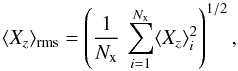 (19)where Nx is the number of individual measurements of ⟨ Xz ⟩ that we obtained, and ⟨ Xz ⟩ i is the ith such measurement. Furthermore, since measurements of the crossover in the stars studied here are often close to the limit of significance, we also consider their reduced χ2,
 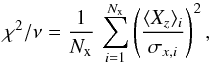 (20)where σx,i is the error of the ith measurement of the crossover. The reduced χ2 is useful in marginal cases to decide if crossover has actually been detected.
As for the longitudinal field, the crossover measurements presented here are considerably more precise than the older determinations of Mathys (1995a) and Mathys & Hubrig (1997). Indeed, the median of the standard errors σx of all the measurements appearing in Table 6 is 848 km s-1 G, while the median of the standard errors of the 44 measurements of the crossover in Ap stars with magnetically resolved lines of the above-mentioned previous studies is 1557 km s-1 G. Close to the detectability limit, this difference of precision may be very significant. Accordingly, in Table 17, we give the values of Nx, ⟨ Xz ⟩ rms, and χ2/ν both for the new measurements of this paper (in Cols. 2 to 4) and for all the existing measurements of the crossover (in Cols. 5 to 7). For the sake of clarity, data in Cols. 5 to 7 appear only for those stars for which previous measurements of the crossover do exist.
Summary of crossover measurements in Ap stars with resolved magnetically split lines.
When the χ2 statistic indicates that crossover is detected at the 99% confidence level, the corresponding entry appears in italics in the table. Such a detection is achieved in 12 of the 34 stars for which CASPEC Stokes V spectra were recorded. Seven of these 12 stars have rotation periods that are shorter than 50 days, similar to all the stars in which crossover had been observed in previous studies (Mathys 1995a; Mathys & Hubrig 1997). We were able to compute, for five of these (relatively) short period stars–namely, HD 81009, HD 137909, HD 142070, HD 144897, and HD 208217 – a formally significant fit of the observed values of ⟨ Xz ⟩ against rotation phase, of one of the forms given in Eqs. (16) or (17) (see Table 10). The independent term of the fit, X0, is not significantly different from 0 in HD 81009, HD 142070, and HD 208217, and only marginally non-zero (at the 3.0σ level) in HD 137909. Also, in these four stars, the difference φX1−φZ1 between the phase origins of the fundamental components of the fits of ⟨ Xz ⟩ and ⟨ Bz ⟩, respectively, is equal to 0.25 within their uncertainties. In other words, the variations of the crossover are lagging behind those of the longitudinal field by a quarter of a cycle. Thus, these stars display the typical behaviour of the rotational crossover, as observed so far in all Ap stars in which the variation of this field moment throughout the rotation period was studied, but HD 147010 (Mathys 1995a; Mathys & Hubrig 1997).
The behaviour observed in HD 144897 is very different. The ⟨ Xz ⟩ measurements are best fitted by a sinusoid with twice the rotation frequency of the star without a fundamental component. Although not visually compelling (see Fig. A.52), this fit appears to be very significant with a value of X2 determined at the 4.4σ level. The ⟨ Bz ⟩ variation curve also seems to show some degree of anharmonicity: while the fit coefficient Z2 is not formally significant (at the 2.7σ level), a fit including it is visually better than a fit by the fundamental alone (see Fig. A.52). Within the errors, the derived phase difference φX2−φZ2 is consistent with a phase lag of 0.125 rotation cycle of the crossover variations with respect to the longitudinal field, as previously observed for the first harmonic in other cases (Mathys 1995a). What is unusual in HD 144897, though, is that the independent term of the fit, X0, is positive, at a high level of significance, 6.9σ. As a matter of fact, the crossover in HD 144897 is never signficantly negative. This is a behaviour that had never been seen in any other star. It is definitely incompatible with the process of rotational crossover in a star in which the magnetic field is symmetric about a plane containing the rotation axis, which is a condition fulfilled by most analytic models successfully used until now to represent Ap star magnetic fields. Actually, it is not clear that the behaviour observed in HD 144897 can be explained by the occurrence of rotational crossover for any plausible magnetic configuration.
In the other two short period stars where the χ2 test indicates that crossover is detected above the 99% confidence level, HD 70331 and HD 116114, its variability is ill-defined, as is that of the longitudinal field. In HD 70331, the individual measurements are distributed between negative and positive values. The apparent predominance of negative ⟨ Xz ⟩ values in HD 116114 may just reflect their marginal significance and their uneven distribution over the stellar rotation period; see below, however.
There is one more short period star, for which a fit of the ⟨ Xz ⟩ variations at the threshold of formal significance (X1/σX1 = 3.0) can be obtained, although crossover is detected only at a confidence level of 70%, according to the χ2 statistic; this star is HD 318107. The ⟨ Xz ⟩ fit is not inconsistent with the standard crossover behaviour, X0 = 0 and φX1−φZ1 = 0.25. However one should in keep in mind that we obtained only six determinations of the crossover in this star, so that the fit has only 3 degrees of freedom.
No crossover was detected in the last star with period shorter than 50 d that was observed with CASPEC as part of this project, HD 335238, for which, however, only three determinations were performed.
In three stars with intermediate periods in Table 17, crossover is detected at the 99% confidence level: these are HD 126515 (P = 130 d), HD 2453 (P = 521 d), and HD 93507 (P = 556 d). Crossover had not been previously detected in stars with such long periods, but the following order of magnitude estimates suggest that the observed effect may still be consistent with the rotational crossover interpretation. It is easy to show from the definitions of the rotational crossover and of the mean magnetic field modulus, that for a given star, at any phase, the following inequality is verified:  (21)Thus, in order for the observed crossover to be consistent with the rotational crossover interpretation, a necessary condition is that
  (22)where the subscripts refer to the maximum of the considered moments over the rotation period. For the crossover, the absolute value is used. For practical application of this condition, we adopt the largest of the individual measurements of the crossover (in absolute value) for | ⟨ Xz ⟩ | max, and of the mean field modulus for ⟨ B ⟩ max. For the crossover, we restrict ourselves to the consideration of the measurements of this paper, since as discussed above, earlier measurements may be considerably less precise. In this way, the minimum values that we derive for v sini are 0.24 km s-1 for HD 126515, 0.27 km s-1 for HD 2453, and 0.50 km s-1 for HD 93507. The necessary condition (22) can be expressed in terms of the stellar radius R (in units of solar radii), by application of the well-known relation between the latter, v sini (in km s-1) and the stellar rotation period P (in d), i.e.
  (23)We find that for HD 126515, R sini ≥ 0.6 R⊙; for HD 2453, R sini ≥ 2.8 R⊙; and for HD 93507, R sini ≥ 5.5 R⊙. These lower limits for HD 126515 and HD 2453 are consistent with the typical values of the radii of stars of their spectral types. They also compare well with the radius estimates obtained from Hipparcos-based luminosity determinations by Hubrig et al. (2000): R = (2.97 ± 0.46) R⊙ for HD 2453, and R = (2.35 ± 0.42) R⊙ for HD126515. For HD 93507, the derived lower limit of the radius is somewhat high for a star of spectral type A0. However taking the involved uncertainties into account, this does not decisively rule out rotational crossover as the source of the observed behaviour. Indeed, if one uses for | ⟨ Xz ⟩ | max and ⟨ B ⟩ max the values computed from the fits of the variations of the crossover (Table 10) and of the field modulus (Table 8) instead of the largest measurement of each of these moments, the resulting lower limit on R sini decreases to (3.8 ± 1.2) R⊙, which is marginally compatible with the spectral type of HD 93507.
Thus HD 126515, HD 2453, and HD 93507 fulfil at least one necessary condition for their observed crossover to be consistent with the classical interpretation of the effect in terms of rotational crossover. In the case of HD 126515, this interpretation receives further support from the observation by Carrier et al. (2002) of radial velocity variations due to approaching and receding inhomogeneities on the stellar surface. By contrast, for HD 93507, the fact that the curves fitted to our longitudinal field data, on the one hand, and to our crossover measurements, on the other hand, vary in phase rather than in quadrature, raises some difficulties. We shall come back to this point below.
The remaining two stars of Table 17 in which crossover is detected at the 99% confidence level, HD 965 and HD 55719, have very long periods. For those stars, identification of the origin of the effect is challenging. The same radius lower limit test as above applied to these two extremely slow rotators (with the values of their rotation periods set to a conservative common lower limit of 10 yr) definitely rules out rotational crossover as the source of the observed effect: R sini ≥ 49 R⊙ for HD 965 and R sini ≥ 32 R⊙ for HD 55719.
HD 94660 may be another example of an extremely slow rotator showing crossover. The χ2 statistic supports the reality of the detection of the effect at a confidence level between 90%, if all the available crossover measurements are considered, and 98%, if the χ2 test is restricted to the better determinations presented in this paper. In addition, the amplitude of a fit of the ⟨ Xz ⟩ data by a function of the form given in Eq. (16) is significant at the 3.5σ level. The correlation coefficient R also supports the existence of a correlation between ⟨ Xz ⟩ and the rotation phase at a confidence level of 99%. Using the value of the stellar radius published by Hubrig et al. (2000), R = (3.15 ± 0.40) R⊙, we can invert the argument of the previous paragraphs to derive an upper limit of the crossover that is compatible with the field modulus of the star, ⟨ Xz ⟩ ≤ (50.6 R/P) ⟨ B ⟩ max = (364 ± 46) km s-1. Strikingly, this limit is within a factor of ~2 of the actually observed values. Taking the uncertainties and approximations involved in this comparison into account, this actually suggests that it is not implausible, although rather unlikely, that rotational crossover is detected in HD 94660. This is further supported by the fact that, based on the fit parameters shown in Tables 9 and 10, the phase lag between the crossover variation and that of the longitudinal field amounts, within errors, to a quarter of a cycle.
As pointed out in Appendix A, for stars for which a sufficient number of measurements of the crossover have been obtained as part of the present study3, the fact that all those measurements, but possibly one or two, yield values of ⟨ Xz ⟩ with the same sign also represents an indication that the effect is actually detected, even though none of these values taken individually reach the threshold of significance. The stars in which this applies are HD 965, 2453, 116114, 116458, and 187474, in which (almost) all ⟨ Xz ⟩ determinations are negative, and HD 93507 and 144897, where the crossover is found to be (almost) always positive. For five of these seven stars, the χ2 test also indicates that crossover was detected at the 99% confidence level. The exceptions are HD 187474, for which the χ2 statistic indicates a non-zero crossover at the 70% confidence level (based on all available measurements; this drops to 50% if only the new determinations of this paper are considered), and HD 116458, where the χ2 value corresponds to a detection at the 70% confidence level (for either the whole set of existing ⟨ Xz ⟩ measurements, or a subset restricted to the new data of this paper).
The usage of the χ2 statistic to decide in marginal cases if crossover has indeed been detected rests on the implicit assumption that the only significant errors affecting the measurements are of statistical nature, to the exclusion of systematic errors. Moreover, systematic errors could plausibly account for the fact that all the crossover measurements in a star in which this effect is very small yield values of the same sign. The following arguments support the view that the crossover determinations of this paper are not significantly affected by systematic errors.
No crossover is detected in more than half of the studied stars. For a number of these stars, the rms crossover is considerably smaller than in any of the stars in which detection is achieved. For instance, in the stars HD 29578, 134214, and 201601, which have all been measured six times or more, ⟨ Xz ⟩ rms is 302, 390, and 257 km s-1 G, respectively. By contrast, all the stars in which the χ2 test indicates the presence of a crossover at the 99% confidence level, have ⟨ Xz ⟩ rms twice as large or (much) more.
Also, for those stars in which (almost) all the crossover data have the same sign, we consider the average ⟨ Xz ⟩ av of all the crossover measurements in a given star, weighted according to their relative uncertainties σx (see Eq. (16) of Mathys 1994). For the most marginal cases of HD 116458 and HD 187474, this average is (− 514 ± 118) km s-1 G and (− 505 ± 165) km s-1 G, respectively. These values can again be compared with those obtained for HD 29578, which is ⟨ Xz ⟩ av = (0 ± 87) km s-1 G, HD 134214, which is ⟨ Xz ⟩ av = (−296 ± 118) km s-1 G, and HD 201601, which is ⟨ Xz ⟩ av = (−80 ± 112) km s-1 G. This comparison represents a strong indication that the systematic measurement of a negative crossover in HD 116458 and HD 187474, and the formally significant non-zero average ⟨ Xz ⟩ av in each of them, are not the result of systematic errors in the measurements, and that they instead reflect the occurrence of some physical process. This conclusion also applies of course to the other stars in which (almost) all the measurements of the crossover have the same sign and in which, furthermore, the χ2 test supports the reality of the detection of a crossover.
The fact that the constant sign of the crossover is positive in some of these stars, and negative in others, represents an additional argument against the suspicion that the constant sign in any star may be due to systematic measurement errors.
Thus we established that the crossover measurements presented here are unlikely to be significantly affected by systematic errors large enough to lead to spurious detections. We built an inventory of the stars in which our CASPEC observations yield definite or probable crossover detections. We discussed the reliability of these detections. We showed that in most stars, the observations can be interpreted in terms of rotational crossover. Remarkably, some of the stars to which this interpretation is applicable rotate very slowly. In previous studies, the star with the longest rotation period in which crossover had been detected at a high level of confidence was HD 81009 (Mathys & Hubrig 1997) with a period of 34 d. With the better data analysed in this study, we showed that rotational crossover is almost certainly detected in a star with period longer than 100 days (HD 126515, P = 130 d); that it may be detectable in stars with periods of the order of 500 d (such as HD 2453); and that it may even plausibly have been observed in HD 94660, which has a period of 7.7 yr. Our data are insufficient to draw definitive conclusions for either HD 2453 or HD 94660, but the discussion of these cases in the previous paragraph clearly indicates that it is not unrealistic with current observational facilities to observe rotational crossover in stars with rotation periods of several years.
Yet, some of the fairly definite crossover detections reported here are inconsistent with the rotational crossover mechanism. The most challenging examples are HD 965 and HD 55719, which rotate too slowly to generate Doppler shifts of the order of magnitude required to account for the measured values of ⟨ Xz ⟩. As long as the local emergent Stokes V line profiles at any point of the stellar surface are anti-symmetric, the apparence of crossover in disk-integrated observations implies the presence of some macroscopic velocity field that is variable across the stellar surface, in a way that some large-scale correlation pattern exists between the Doppler shift that it generates and the Zeeman effect across the stellar surface. The effects that can generate departures from Stokes V anti-symmetry at a given point of the stellar surface have been discussed by Mathys (1995a). Two of these effects, non-LTE populations of the magnetic substates of the levels involved in the observed transitions and the partial Paschen-Back effect in these transitions, can almost certainly be ruled out for the studied spectral lines in the stars of interest. The third effect, which is the existence of velocity gradients along the line of sight in the line-forming region (Landi Degl’Innocenti & Landolfi 1983), represents another form of Doppler-Zeeman combination. Thus the need for a velocity field of some kind appears inescapable.
One well-known type of velocity field that is definitely present in (cool) Ap stars is non-radial pulsation, which furthermore has a large-scale structure that makes it a priori suitable for the generation of correlations across the stellar surface between the Doppler shifts resulting from it and the local Zeeman effect. At first sight, there are several arguments against the hypothesis that this mechanism may be responsible for the observed crossover. The effective temperature of HD 55719, an A3 star, is close to, or above the upper limit of the temperature range to which all rapidly oscillating Ap (roAp) stars known so far are confined. By contrast, HD 965 has all the characteristics of typical roAp stars, but all efforts so far to detect pulsation in this star have been unsuccessful (Elkin et al. 2005a). Also, the integration times that were used to record the CASPEC spectra of HD 965 analysed here, ranging from 25 to 40 min, are longer than the typical pulsation periods of roAp stars, which for the stars known so far range from 5 to 24 min. Thus one would expect the disk-integrated radial velocity variations to average out to a large extent. This does not apply to HD 55719, which is much brighter than HD 965, and for which the exposure times of our CASPEC observations exceeded 5 min only on a single cloudy night.
However, the pulsation amplitude in roAp stars varies across the depth of the photosphere (e.g. the introduction of Kurtz et al. 2006, for an overview). The most obvious observational manifestation of this depth effect is the existence of systematic amplitude differences in the radial velocity variations of lines of different ions or of lines of different intensities of a given ion. In particular, it is not unusual for a subset of spectral lines not to show any radial velocity variations due to pulsation; this indicates the presence of at least one pulsation node in the photospheres of roAp stars. In first approximation, the photospheric depth dependence of pulsation is inferred from the observed radial velocity amplitudes by assuming that each line forms at a single depth. This is, of course, an oversimplification: line formation actually takes place over a range of optical depths.
For the purpose of the present discussion, the important consequence is that in roAp stars, there are indeed radial velocity gradients along the line of sight in the line-forming region, which may generate local emergent Stokes V line profiles that are not anti-symmetric. This departure from anti-symmetry is a radiative transfer effect whose calculation is non-trivial (Landolfi & Landi Degl’Innocenti 1996). The details of this calculation are unimportant here. The relevant point is that one can show very generally that such a departure from anti-symmetry of the local emergent Stokes V line profiles can produce a non-zero second-order moment of the observable, disk-integrated Stokes V profiles even in a non-rotating star, which does not cancel out in exposures integrated over a pulsation period (see Appendix C for details). Hence this is a mechanism that can generate crossover in stars that have negligible rotation. In what follows, we refer to this as pulsational crossover.
The defining feature for the appearance and the sign of this crossover is the location in the photospheric layer of the region of formation of the diagnostic lines with respect to that of the pulsation nodes, which in general should not vary much across the stellar surface. Hence, one can expect that, in most cases, pulsational crossover keeps the same sign throughout the rotation period. Some rotational modulation could plausibly occur; in stars where the magnetic field is approximately symmetric about an axis passing through the stellar centre, this modulation should be in phase (or in antiphase) with the longitudinal field variation. Finally, since the departure from anti-symmetry of the local Stokes V line profiles does not cancel out when averaged over the stellar disk, pulsational crossover observations may actually be sensitive to pulsations corresponding to spherical harmonics Yℓm of higher degree ℓ than those that can be detected through photometric or radial velocity observations.
Thus, with the pulsational crossover, we identified a mechanism, which at least qualitatively can account for all the observed features of the crossover data presented here that cannot be explained by the classical rotational crossover. These observed features of the crossover data are the following:
-
1.
the detection, at a high level of confidence, of non-zerocrossover in extremely slow rotators (HD 965,HD 55719);
-
2.
the occurrence of non-reversing crossover (HD 2453, HD 93507, HD 116114, HD 144897; possibly also HD 965, HD 116458, and HD 187474);
-
3.
the absence of a phase lag between the longitudinal field and crossover variations (HD 93507).
However, this interpretation is sustainable only for stars where non-radial pulsations similar to those of roAp stars occur. Among the examples given above, only HD 116114 is an established roAp star (Elkin et al. 2005b). HD 187474 showed no evidence of pulsation in the Cape Photometric Survey (Martinez & Kurtz 1994), and neither did HD 2453 in the Nainital-Cape Survey (Joshi et al. 2009). We did not find in the literature any report of attempts to detect pulsation in HD 93507 or HD 144897. The null results for HD 965, HD 2453, and HD 187474 do not necessarily rule out the interpretation of their crossover as being due to pulsation, as pulsational crossover is sensitive to harmonics of higher degree ℓ than photometry or radial velocities. Also, the fact that HD 2453, HD 55719, HD 93507, HD 116458, HD 144897, and HD 187474 are hotter than all roAp stars known to date does not represent a definitive argument against the occurrence of non-radial pulsations in these stars. As a matter of fact, some of these stars have effective temperatures and luminosities (e.g. Hubrig et al. 2000) that place them within the boundaries of the Cunha (2002) theoretical roAp instability strip.
As mentioned previously, numerical modelling of the radiative transfer effects that are invoked in the pulsational crossover interpretation is nontrivial. Given the uncertainties involved on the structure of the magnetic field and of the pulsation, such modelling may not allow one to establish on a quantitative basis if the proposed pulsational crossover mechanism is adequate to explain the type of effect found in the data presented here. Further observations should provide more critical tests of this mechanism. For instance, in slowly rotating roAp stars, determinations of the crossover from sets of diagnostic lines of different ions, formed in optical depth ranges located differently with respect to photospheric pulsation nodes, should yield different results, possibly even of opposite sign in some cases. Or, in time series of Stokes V spectra of roAp stars with a time resolution that is short compared to their pulsation period, the crossover should be found to vary with the pulsation frequency.
Of course, rotational crossover and pulsational crossover are not mutually exclusive, and in stars with moderate, but non-negligible rotation, the observed effect may actually be a combination of both. Of the stars studied here, HD 137909 may possibly show the result of such a combination, with a dominant rotational crossover component varying in phase quadrature with the longitudinal field, and a weaker pulsational crossover component responsible for the formally significant non-zero value of X0. We mention this possibility here for illustrative purposes, rather than as a firm statement that both rotational and pulsational crossovers are definitely detected in the star. Such a statement would be an overinterpretation of a marginally significant observational result.
As hinted above, even though observation of pulsational crossover is mostly restricted to very slowly rotating stars, this effect could potentially be a valuable diagnostic to detect in magnetic Ap stars non-radial pulsations that are not detectable via more traditional approaches such as photometric or radial velocity variations, for example because they correspond to harmonics with a higher degree ℓ, for which local photometric or radial velocity variations average out in disk-integrated observations. Such higher degree pulsations in Ap stars represent unexplored territory.
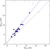 |
Fig. 12 Observed average of the mean quadratic magnetic field against the observed average of the mean magnetic field modulus. Open symbols are used to distinguish those stars for which either or both of ⟨ Bq ⟩ av and ⟨ B ⟩ av were computed using less than 7 individual measurements of ⟨ Bq ⟩ and ⟨ B ⟩, respectively. The short-dashed line corresponds to ⟨ Bq ⟩ av = ⟨ B ⟩ av. The long-dashed line represents the least-squares fit of the observed relation between ⟨ Bq ⟩ av and ⟨ B ⟩ av; it is based only on the stars for which at least 7 measurements of both ⟨ Bq ⟩ and ⟨ B ⟩ are available. |
5.4. The mean quadratic magnetic field
As for the longitudinal field and the crossover, the precision of the new mean quadratic magnetic field measurements of this study is significantly better than the precision of older determinations of this field moment from CASPEC spectra. The median of the standard errors σq of the 229 ⟨ Bq ⟩ measurements reported in Table 6 is 336 G. For the 40 measurements of this field moment in Ap stars with resolved magnetically split lines that were published by Mathys (1995a) and Mathys & Hubrig (1997), this median was 581 G.
In Col. 10 of Table 13, we give for each star the average value ⟨ Bq ⟩ av of the mean quadratic field measurements of this study and of the previous works of Mathys (1995b) and Mathys & Hubrig (1997). The total number of these measurements, Nq, appears in Col. 9. For HD 134214 and HD 201601, Mathys & Hubrig (1997) could not determine a physically meaningful value of ⟨ Bq ⟩ at some epochs, so that Nq < Nz. Moreover, as already mentioned, the quadratic field of HD 188041 is too small to allow any meaningful quantitative information to be derived about it at any epoch.
In Fig. 12, we plot ⟨ Bq ⟩ av against the average of the mean magnetic field modulus values ⟨ B ⟩ av. The short-dashed line corresponds to ⟨ Bq ⟩ av = ⟨ B ⟩ av. At any given phase, the mean quadratic field must be greater than or equal to the mean field modulus: ⟨ Bq ⟩ > ⟨ B ⟩, by definition of the quadratic field (see Mathys & Hubrig 2006). This does not strictly imply that a similar relation should be satisfied between the averages of our measurements of these two field moments for each star individually because the field modulus and quadratic field data considered here sample different sets of rotation phases of the studied stars. But on a statistical basis, given that the epochs of the considered observations can be regarded as random with respect to the rotation phases of all the stars of our sample, the relation ⟨ Bq ⟩ av > ⟨ B ⟩ av should be fulfilled. The fact that, in Fig. 12, the representative points of the majority of the stars fall above the ⟨ Bq ⟩ av = ⟨ B ⟩ av line (short-dashed line) is fully consistent with this expectation.
Actually, considering only the stars for which at least seven determinations of both ⟨ Bq ⟩ and ⟨ B ⟩ are available (which are represented by filled symbols), one can note in the figure the existence of a nearly linear relation between ⟨ B ⟩ av and ⟨ Bq ⟩ av, with a steeper slope than the ⟨ Bq ⟩ av = ⟨ B ⟩ av line. We estimated this slope to be 1.28 from a least-squares fit of the data; in Fig. 12, this fit is represented by the long-dashed line. This value is reasonably consistent with the assumption that underlies the quadratic field determinations. Indeed the latter implies that ⟨ Bq ⟩ 2 = 1.33 ⟨ B2 ⟩ ≥ 1.33 ⟨ B ⟩ 2, hence ⟨ Bq ⟩ ≥ 1.15 ⟨ B ⟩. This consistency, and the fact that the deviations of individual points from the best fit line are moderate at most, give us confidence that the quadratic field values that we obtain are realistic. In particular, these results obtained from the analysis of a large number of ⟨ Bq ⟩ determinations indicate that the tendency of the applied method to underestimate the quadratic field, identified by Mathys & Hubrig (2006), is moderate at most. Conversely, there is no indication in the present results that the quadratic field may have been significantly overestimated in any star. These conclusions, which are based on the largest set of ⟨ Bq ⟩ determinations ever performed, confirm that the quadractic field is a good diagnostic of the intrinsic strength of Ap star magnetic fields, at least on a statistical basis. This diagnostic should be particularly useful in stars with moderate rotation in which spectral lines are not magnetically resolved because their Doppler broadening exceeds their Zeeman splitting.
For 8 stars, we obtained ⟨ Bq ⟩ measurements distributed sufficiently well across the rotation period so as to allow the variation of this field moment to be characterised. We fitted the variation curves of the quadratic field of these stars by functions of the forms given in Eqs. (16) or (17). The fit parameters are given in Table 11. The formal significance of the amplitude Q2 of the first harmonic of the fit is below the 3σ level for the four stars of this table for which it was included. This is the case even though for all of these stars, the inclusion of the first harmonic significantly improves both the reduced χ2 and the multiple correlation coefficient R with respect to a fit by a single cosine with the stellar rotation frequency. Furthermore, for HD 2453, even the fit by the fundamental is not formally significant, since Q1/σ(Q1) = 2.5. This fit was included in Table 11 only on account of the fact that visually it appears rather convincing (see Fig. A.2).
For these 8 stars, we computed from the fits the ratio p = ⟨ Bq ⟩ max/ ⟨ Bq ⟩ min of the maximum to the minimum of the quadratic field. The resulting values appear in the last column of Table 13. For those stars for which it was not possible to compute a significant fit of the variations of this field moment, contrary to the field modulus and to the longitudinal field, we do not regard the ratio of the highest to the lowest measured value of ⟨ Bq ⟩ as a reliable indicator of its amplitude of variation. Indeed, a formally significant fit of the variations of the quadratic field could only be computed for 7 of the 16 stars for which this could be performed for the variation of the longitudinal field because the relative uncertainties of the ⟨ Bq ⟩ measurements with respect to the amplitude of their variations are much greater than for the ⟨ Bz ⟩ data. Comparison of the fit parameters Z1 and Q1 in Tables 9 and 11 shows that in their majority, their orders of magnitude are fairly similar. By contrast, the median of the standard errors of the field moment determinations is ~7 times as large for the quadratic field as for the longitudinal field. Accordingly, in many cases, the difference between the highest and lowest individual values of ⟨ Bq ⟩ in a given star is more representative of the measurement errors than of the actual variation of this field moment.
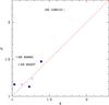 |
Fig. 13 Relative amplitude p of the mean quadratic magnetic field variations against that of the mean magnetic field modulus variations (q). Open symbols: stars showing ⟨ Bz ⟩ reversal; filled symbols: stars in which ⟨ Bz ⟩ has a constant sign. Among the latter, triangles are used to distinguish those stars in which the phase of maximum ⟨ B ⟩ coincides approximately with the phase of lowest absolute value of ⟨ Bz ⟩, while dots are used when ⟨ B ⟩ maximum occurs close to the phase of highest absolute value of ⟨ Bz ⟩. |
Given the correlation between quadratic field and field modulus illustrated in Fig. 12 (see also Mathys & Hubrig 2006), we would expect the amplitudes of variation of these two quantities to be related to each other. To check this, we have plotted p = ⟨ Bq ⟩ max/ ⟨ Bq ⟩ min against q = ⟨ B ⟩ max/ ⟨ B ⟩ min in Fig. 13. The dashed diagonal line represents the locus p = q. While most points cluster around it, three appear considerably above, corresponding to the stars HD 93507, HD 94660, and HD 126515. Both HD 93507 and HD 94660 have non-reversing longitudinal fields with the phase of the lowest absolute value of ⟨ Bz ⟩ roughly coinciding with the maximum of the field modulus. As discussed in Sect. 5.2, this indicates that the magnetic fields of these stars have structures significantly departing from centred dipoles. Similarly, HD 126515 is one of very few stars known whose longitudinal field variation curve shows pronounced anharmonicity, reflecting a considerable departure from a centred dipole. As a result of such a departure, the variation of the magnetic field strength across the stellar surface may be larger than for a centred dipole.
The quadratic field is defined as ![Mathematical equation: \begin{eqnarray} \Hq&=&(\av{B^2}+\av{B_z^2})^{1/2}\nonumber\\ &=&\left[\Hm^2+\sigma^2(B)+\Hz^2+\sigma^2(B_z)\right]^{1/2}, \label{eq:Hqdef} \end{eqnarray}](/articles/aa/full_html/2017/05/aa28429-16/aa28429-16-eq654.png) (24)where σ2(B) and σ2(Bz) are the standard deviations across the visible stellar disk of the local values of the modulus and the line of sight components of the magnetic vector, respectively. In general, these standard deviations become greater when the field structure shows significant departures from a centred dipole. The resulting increase of their contribution to the quadratic field, which is phase dependent, may possibly account for the large amplitude of variation of ⟨ Bq ⟩ compared to ⟨ B ⟩ in HD 93507, HD 94660, and HD 126515. However, in the latter two stars, the maximum of the quadratic field is only constrained by old measurements of Mathys (1995b) and Mathys & Hubrig (1997), which are much less precise and reliable than those of the present study. Consideration of Figs. A.34 and A.42 suggests indeed that the value of p for these two stars may be affected by significant uncertainties. The phase sampling of our new ⟨ Bq ⟩ measurements of HD 93507 is better, but as noted in Appendix A.18, the distortion of the spectral lines around the phase of maximum of ⟨ B ⟩ increases the measurement errors of all field moments, and hence, the uncertainties affecting both p and q as well. On the other hand, the line distortion is also suggestive of the presence of a significant small-scale structure in the local magnetic field in the corresponding region of the stellar surface, which in turn could account for a large amplitude of variation of the quadratic field, compared to the mean field modulus.
(24)where σ2(B) and σ2(Bz) are the standard deviations across the visible stellar disk of the local values of the modulus and the line of sight components of the magnetic vector, respectively. In general, these standard deviations become greater when the field structure shows significant departures from a centred dipole. The resulting increase of their contribution to the quadratic field, which is phase dependent, may possibly account for the large amplitude of variation of ⟨ Bq ⟩ compared to ⟨ B ⟩ in HD 93507, HD 94660, and HD 126515. However, in the latter two stars, the maximum of the quadratic field is only constrained by old measurements of Mathys (1995b) and Mathys & Hubrig (1997), which are much less precise and reliable than those of the present study. Consideration of Figs. A.34 and A.42 suggests indeed that the value of p for these two stars may be affected by significant uncertainties. The phase sampling of our new ⟨ Bq ⟩ measurements of HD 93507 is better, but as noted in Appendix A.18, the distortion of the spectral lines around the phase of maximum of ⟨ B ⟩ increases the measurement errors of all field moments, and hence, the uncertainties affecting both p and q as well. On the other hand, the line distortion is also suggestive of the presence of a significant small-scale structure in the local magnetic field in the corresponding region of the stellar surface, which in turn could account for a large amplitude of variation of the quadratic field, compared to the mean field modulus.
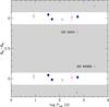 |
Fig. 14 Phase difference φQ1−φM1 between the fundamenals of the fits of the measurements of ⟨ Bq ⟩ and ⟨ B ⟩ by functions of the forms given in Eqs. (16) and (17), against stellar rotation period. The meaning of the symbols is the same as in Fig. 13. Shaded zones correspond to forbidden regions where points are not expected to be found (see text for details). Two stars that depart from this expected behaviour (one of them marginally) are identified. |
The phase difference φQ1−φM1 between the fundamental components of the fits to the variation curves of ⟨ Bq ⟩ and ⟨ B ⟩ (see Table 11) is plotted against the stellar rotation period in Fig. 14. For magnetic field structures symmetric about an axis going through the centre of the star, the quadratic field should vary in phase with the mean field modulus. To visualise this in Fig. 14, the forbidden region corresponding to 0.1 ≤ φQ1−φM1 ≤ 0.9 is shaded. Of the two representative points lying in this shaded region, only the one corresponding to HD 94660 identifies a phase lag in the 0.1 ≤ φQ1−φM1 ≤ 0.9 band at a formally significant level (3.4 σ). As mentioned above, this star has a magnetic field whose structure significantly departs from a centred dipole. Actually, the variations of its field modulus indicate without any doubt that its field is not symmetric about an axis passing through the centre of the star. Thus despite the poor definition of the phase of maximum of the quadratic field of this star resulting from the lack of new, precise ⟨ Bq ⟩ measurements around it, it is quite plausible that the non-zero φQ1−φM1 difference is real and significant. On the other hand, while the non-zero value of this difference for HD 2453 may also appear significant from consideration of its error bar, one must keep in mind that the amplitude of the ⟨ Bq ⟩ fit is not formally significant.
Thus the statistical conclusions that can be drawn from the quadratic field measurements are limited by the incomplete phase coverage of the new determinations of this paper in many stars (especially, those with very long rotation periods) and by the moderate precision of the older data of Mathys (1995b) and Mathys & Hubrig (1997).
On the other hand, while in principle one can also determine the projected equatorial velocity from the analysis of the second-order moments of the Stokes I line profiles (see Mathys & Hubrig 2006), the contribution of the rotational Doppler effect to the line profiles of the majority of the stars with magnetically resolved lines is too small to allow significant constraints on v sini to be derived from observations at the moderately high resolution of CASPEC.
5.5. Rotation
Based on the new magnetic field determinations presented in this paper, we were able to derive new constraints on the rotation periods of 21 stars. For four of these stars, the rotation period was determined for the first time, and for a fifth star, a first lower limit of its value was tentatively obtained. The recent determination of the period of HD 18078 by Mathys et al. (2016) also relies in part on our new ⟨ B ⟩ data. For six stars, the new Prot value reported here only corresponds to an improvement of the accuracy of a previously published value, without significant impact on, for example, the statistical distribution of the rotation periods. By contrast, the lengthening of the time span covered by our measurements, resulting from the combination of the data of Paper I with those discussed here, allowed a considerably increased lower limit of the rotation period to be set for seven stars. For two more stars, HD 965 and HD 166473, Prot lower limits substantially higher than in Paper I, partly based on our new magnetic field measurements, have already been published in separate papers (Elkin et al. 2005a; Mathys et al. 2007).
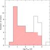 |
Fig. 15 Histogram showing the distribution of the rotation periods of the 50 Ap stars with resolved magnetically split lines for which their value has been determined (shaded part of the histogram) or for which a meaningfully lower limit has been obtained (see text). |
Figure 15 shows the distribution of the rotation periods of the Ap stars with resolved magnetically split lines (see Tables 1 and 2). The shaded part of the histogram corresponds to the 40 stars for which the exact value of the rotation period is known; for the remaining ten stars, only a lower limit could be determined until now. The tentative lower limits quoted in Table 1 for HD 213637 and in Table 2 for HD 92499 and HD 117290 are regarded as too uncertain for inclusion in this accounting.
Unsurprisingly, while up to ~70% of all Ap stars have rotation periods between 1 and 10 days (Mathys 2004), for ~75% of the present sample, the rotation period is longer than 10 days, and all stars but one (for which the value of the period still involves some ambiguity) have rotation periods longer than 3 days. This is obviously a selection effect, as the magnetic splitting of the spectral lines can be observed only in stars with small enough v sini.
Conversely, magnetically split lines should be resolved in the vast majority of the Ap stars with Prot > 10 d, provided that they have a strong enough field (⟨ B ⟩ ≳ 2.5 kG). This suggests that, for rotation periods above ~10 days, the distribution seen in Fig. 15 should be reasonably representative of the long-period tail of the actual distribution of the rotation periods of (strongly magnetic) Ap stars. For more than half of the stars of the rightmost four bins of this distribution (corresponding to Prot > 1000 d), the available magnetic data sample a time interval shorter than the rotation period; this time interval represents a lower limit of the actual period. Accordingly, the secondary peak of the period distribution, between 1000 and 10 000 days, may not be real, but it may just reflect the limited time coverage of the observations of most long-period stars. As time passes by and more measurements are acquired, stars that are currently contributing to that peak may shift to higher bins. Ultimately, the long-period tail of the log Prot distribution may actually prove flat, corresponding to an exponential decrease with the period. Such a decrease would be consistent with a statistical distribution. The actual existence of a secondary peak in the distribution (in the 1000–10 000 day range or higher) cannot definitely be ruled out, but understanding its origin would require some additional, unknown mechanism to be invoked.
For a flat distribution in log Prot scale to be achieved above Prot = 100 d, about 2/3 of the stars currently appearing in the [ 3...3.5 [ and [ 3.5...4 [log Prot bins of the Fig. 15 histogram on the basis of the current lower limits of their periods must actually have rotation periods longer than 104 days. This in turn requires that among the stars for which only a lower limit of the rotation period is known so far, about half populate the [ 4.5...5 [ bin of the histogram. Thus following this line of reasoning strongly suggests that a small but non-negligible number of Ap stars must have rotation periods of the order of 1–3 centuries. The argument developed here represents the first concrete piece of evidence of the probable occurrence of such long rotation periods, which have never been directly measured. As a matter of fact, Belopolsky (1913) achieved the first determination of the period of an Ap star, α2 CVn (Prot = 5.5 d), just one century ago, so that for no such star have the variations been studied over a time span significantly exceeding 100 yr.
There is no reason a priori why the log Prot distribution should become flat at Prot = 100 d. It could plausibly continue to decrease monotonically up to a higher value of the period, then become flat, or even just tend asymptotically towards zero. In either of these alternatives, some stars should eventually populate bin [ 5...5.5 [, or even higher bins, of the histogram. This leads to the conjecture that some Ap stars may have rotation periods ranging from 300 to 1000 yr, or even longer. Obviously, obtaining meaningful constraints on such periods, if they do indeed occur, will represent a major challenge.
An additional constraint on the rate of occurrence of (very) long rotation periods in Ap stars can be derived from consideration of the whole sample of 84 Ap stars with resolved magnetically split lines from Tables 1 and 2. Out of the 50 of these stars for which a reliable value, or lower limit, of the rotation period was obtained, 31 have Prot > 30 d. The remaining 34 stars with magnetically resolved lines were not studied enough to constrain their rotation periods. But there is nothing in the way in which they were discovered that would suggest that the distribution of their periods should be significantly different. Thus, among all the known Ap stars with resolved magnetically split lines, approximately 54 should have rotation periods longer than 30 d.
Conversely, the vast majority of the stars known to have Prot > 30 d show magnetically resolved lines. Of the Ap stars listed in Catalano & Renson (1998) and Renson & Catalano (2001) for which the period definitely exceeds 30 days, only two, HD 8441 and HD 221568, do not show resolved magnetically split lines. Period values greater than 30 days were derived more recently for two more stars with unresolved lines, HD 123335 (Hensberge et al. 2007) and HD 184471 (Kudryavtsev & Romanyuk 2012). But there are a considerable number of Ap stars whose spectral lines show very little, if any, hint of rotational or magnetic broadening, even when observed at a resolving power of the order of 105, and whose period is unconstrained. It is very plausible that a sizeable portion of these stars may have (very) long rotation periods, hence further contributing to increasing the population of the long-period tail of the distribution of the rotation periods of the Ap stars.
The list of critically evaluated values of rotation periods extracted by Mathys (2004) from the Catalano & Renson (1998) catalogue and its 2001 supplement (Renson & Catalano 2001) comprised 23 entries in the range 10–300 days, and eight periods longer than 300 days. Updating it with the reliable new period values or lower limits of Tables 1 and 2 raises these counts to 31 stars with a rotation period between 10 and 300 days (including the above-mentioned HD 123335 and HD 184471), and 21 stars whose period exceeds 300 days. This corresponds to an increase of ~35% in the number of known intermediate length (i.e. 10–300 d) periods and to doubling the number of constrained very long (>300 d) periods. Despite the small number statistics, the much greater relative increase in the population of the group of stars with very long periods represents a significant difference, especially keeping in mind that 2 of the stars of Tables 1 and 2 for which the lower limit of the period is too uncertain for inclusion in the above accounting (HD 92499 and HD 117290) likely have Prot> 300 d, while HD 213637 is the only star in these tables for which the value of the period is still unknown; this value could be between 10 and 300 days. Also, while for nine of the stars of Table 1, the period is definitely of the order of 10 yr or longer, only three of these stars were reported to have such slow variations in the Catalano & Renson (1998) catalogue.
In summary, consideration of the new constraints on the rotation periods of Ap stars that were obtained as part of the systematic study of those stars with resolved magnetically split lines, whose results are reported in Paper I and in this paper, indicates that the long-period tail of their distribution is considerably more populated and likely extends to significantly higher values than was apparent only 15 yr ago.
5.6. Binarity
As explained in Sect. 3.3, realistic estimates of the measurement uncertainties cannot be inferred by the methods used to determine the radial velocity. The external errors (due e.g. to flexures) cannot be evaluated from a comparison of different diagnostic lines for CASPEC observations, while the fact that the radial velocity is obtained from a single line does not even allow the internal errors to be constrained for high-resolution spectra in natural light; this limitation is similar to the one encountered for the mean magnetic field modulus, which was discussed in detail in Sect. 6 of Paper I.
As a workaround, we used the individual differences between the observed values of the radial velocity and those computed from the fitted orbits for the nine stars for which we computed orbital solutions (see Table 12), as follows. We did this separately for the CASPEC data, on the one hand, and for the measurements obtained from high-resolution, unpolarised observations, on the other hand. For both subsets, we considered all nine stars together (only six of these stars were actually observed with CASPEC), and we calculated the rms of the individual differences between measurements and fit in each of them: 0.95 km s-1 in the CASPEC case (from 62 differences) and 0.97 km s-1 in the high-resolution case (from 216 differences). In the latter case, the derived rms likely correctly reflects the actual uncertainties affecting our radial velocity measurements. Accordingly, we adopt 1 km s-1 as the value of the measurement errors for all the instrumental configurations of Table 3. Indeed we did not identify any obvious difference between them with respect to the precision of the radial velocity measurements. However, the vast majority of those measurements were obtained with either the CAT + CES LC configuration at ESO, the AURELIE spectrograph at OHP, or the KPNO Coudé feed. The number of data resulting from observations recorded with other instrumental configurations is too small to allow differences in their precision to be assessed beyond ruling out major discrepancies.
By contrast, we believe that the actual uncertainty of the radial velocity values determined from CASPEC observations is underestimated by their rms difference with the orbital fits; this is probably out of a fortunate coincidence (in particular, such measurements were available for only six of the nine binaries of Table 12). Indeed, visual comparison of the CASPEC-based radial velocity values with those obtained from high-resolution spectra in some stars suggests the existence of systematic differences greater than 1 km s-1 (e.g. HD 29578 in Fig. A.13) as well as a larger scatter than for the high-resolution points (e.g. HD 144897 in Fig. A.53). Based on these considerations, we adopt a value of 2 km s-1 for the errors of the radial velocity measurements obtained from CASPEC spectra.
Both in the CASPEC case and for the high-resolution unpolarised spectra, we assume that the measurement errors are the same for all stars. This approach partly reflects the limitations of our study, such as the fact that exploitation of the radial velocity information was an afterthought. However, it is borne out by the fact that consideration of the various radial velocity curves of Appendix A shows that the scatter of the individual measurement points about the fitted orbits, or about reasonably smooth variation trends, for those stars for which orbital elements could not be computed, is fairly similar in all stars.
Ap stars with magnetically resolved lines with a known orbital period (or a meaningful lower limit thereof).
We identified three additional spectroscopic binaries (SB) among the 43 Ap stars with resolved magnetically split lines for which new observations are presented in this paper; these SBs are HD 144897, HD 165474, and HD 200311. HD 165474 was already flagged as a visual binary in Paper I. Furthermore, our radial velocity measurements confirm and strengthen the inference by Carrier et al. (2002) that HD 2453 and HD 18078 are also spectroscopic binaries, which were not recognised as such in Paper I. By contrast, we point out that the apparent variability of the radial velocity of HD 216018 that we reported in that paper was actually due to spurious determinations. In addition, HD 201601 is a visual binary for which a first, preliminary orbital solution was recently computed (Stelzer et al. 2011). Thus 22 stars out of our sample of 43 are binaries, compared to 18 out of 41 in Paper I. The rate of occurrence of binarity in our sample, 51%, is slightly higher than the values of 43% reported by Carrier et al. (2002) for Ap stars in general, and of 46% derived by Gerbaldi et al. (1985) for the cool Ap stars. This difference is marginal, but it may to some extent reflect the fact that our study is particularly suited to the identification of systems with long orbital periods because of its character (high spectral resolution observations repeated at semi-regular intervals over a time span of several years) and of the nature of our sample (stars with low v sini, for which radial velocities can be determined very precisely). Such systems may escape detection when the primary is rotating faster or in projects carried out on a shorter time span.
Orbital elements were determined for 14 of the 22 binaries of this paper. For three of these binaries (HD 29578, HD 50169, and HD 61468), an orbital solution was obtained for the first time. We also presented revised solutions for five other systems: HD 9996, HD 12288, HD 55719, HD 94660, HD 116458 and HD 187474. For four systems, either orbital elements based on our observations had already been published (HD 59435, HD 81009) or our new data did not allow us to improve determinations that were already based on much more extensive sets of measurements (HD 65339, HD 137909). The last system for which (partial) orbital elements are available, HD 201601, is a visual binary, for which we did not observe radial velocity variations. The relevant references are quoted in the respective sections of Appendix A. For seven other systems, constraints on the orbital periods (mostly lower limits) have been obtained by Carrier et al. (2002) for HD 2453, HD 18078, HD 116114, and HD 142070; and in this paper for HD 144897, HD 165474, and HD 200311. For the last spectroscopic binary, HD 208217, our data are insufficient to characterise the orbit. The main properties of the remaining 21 stars (rotation and orbital periods, or lower limits; eccentricity and mass function) are summarised in Table 18. The reference given in the last column is to the paper where the listed orbital parameters or orbital period estimate were originally published. When they were derived in the present study, there is no entry in this column.
The shortest of the 21 orbital periods that are known or constrained is 27 days long. This is remarkable. While the (almost) complete lack of binaries containing an Ap star with orbital periods shorter than 3 days has long been known (Gerbaldi et al. 1985; Carrier et al. 2002), one can see in Fig. 8 of Carrier et al. that for about one-third of the binaries of their sample with Si or SrCrEu peculiarity type (similar to the stars studied here), the logarithm of the orbital period is less than 1.4 (that is, the period is shorter than 25 days). The difference in the behaviour of the spectroscopic binaries of the present paper is highly significant: if the Carrier et al. sample and ours had similar properties, we would expect our sample to include six or seven binaries with orbital periods shorter than 25 days. Also, the number of spectroscopic binaries considered here is about half the number of Si and SrCrEu stars in the Carrier et al. study. In other words, with an increased number of binaries and an improved knowledge of their orbits, those considerations strengthen our suspicion of Paper I, that the subset of Ap stars with resolved magnetically split lines shows an extreme deficiency of binaries with short orbital periods as compared to the class of the magnetic Ap stars as a whole. In this context, Ap star must be understood in a rather strict sense, that is, roughly limited to spectral type A: formally, our sample ranges from B8p (HD 70331, HD 144897, HDE 318107) to F1p (HD 213637). This should essentially coincide with the Carrier et al. (2002) SrCrEu and Si subgroups, but exclude the He weak and (of course) HgMn stars of their study.
Ap stars with published reliable orbital and rotation periods, not known to show magnetically resolved lines.
On the other hand, recently published preliminary results of a systematic survey of magnetism in binaries with short orbital periods (Porb< 20 d) indicate that less than 2% of the components of spectral types O–F of such systems have large-scale organised magnetic fields (Alecian et al. 2015). While this strongly suggests that the rate of occurrence of such fields is considerably lower in close O–F binaries than in single stars of similar spectral type, it is not inconsistent with the results of Carrier et al. (2002). Indeed the sample of the latter study consists of stars that were initially selected for their chemical peculiarity, so that it comprises only a rather small fraction of the whole set of binary stars of spectral type A. Conversely, as can be seen in Fig. 1 of Alecian et al. (2015), only about 1/3 of the stars of their sample have spectral types between early F and late B, and the rate of occurrence of magnetism may not be uniform throughout the all range of spectral types covered by their sample.
In order to gain further insight into the nature and origin of the apparent deficiency of short-period spectroscopic binaries among the Ap stars with resolved magnetically split lines as compared to the Carrier et al. (2002) sample, we looked in the literature for other Ap stars in binaries for which both the orbital and rotation periods are known. We critically assessed the reliability of the published periods, checking the original papers in which they were derived. To our surprise, we only identified 12 stars for which we felt confident that the values of both periods were established firmly enough to warrant consideration. Their properties are summarised in Table 19. Most columns should be self-explanatory. The source of the rotation periods is identified by the references in Col. 5; Col. 9 lists the papers in which the orbital elements were originally published.
Some caution must be exerted with respect to three of the stars in Table 19. Their HD numbers appear in italics and we also use italics to identify the corresponding elements of information that are subject to reservations. The listed value of the rotation period of HD 25267 satisfactorily represents the variations of its mean longitudinal magnetic field observed by Borra & Landstreet (1980). However Manfroid et al. (1985) found this value of the period inconsistent with their photometric observations. But the interpretation of these observations, which indicate the presence of two periods of variation (1.2 d and 3.8 d), has remained unclear to this day. On the other hand, the Leone & Catanzaro (1999) argument that the observed variations of the longitudinal field, between −400 G and 0 G, are incompatible with a value close to 90° of the angle i between the rotation axis and line of sight, is weak. The non-reversal of this field moment only requires that i + β ≤ 90° and the example of HD 142070 (Appendix A.28) shows that ⟨ Bz ⟩ variation amplitudes of several hundred Gauss may be observed even when either i or β (the angle between the rotation and magnetic axes) is only a few degrees. Carrier et al. (2002) cannot definitely rule out a period alias very close to 1 day for the radial velocity variations of HD 191654, which would then be due to rotation. However, the 2121 d alternative corresponding to an orbital motion seems more plausible, especially since the photometric period of 1 85 (Vetö et al. 1980) appears robust and can very plausibly be attributed to rotation. Finally, the spectral subtype of the Bp primary of HD 123335, and its temperature, may possibly be above the upper limit of the range covered by the stars of our sample, as specified in page .
Although Gerbaldi et al. (1985) list several other cool Ap and Si stars as having known orbital and rotation periods, none of these stars stand up to closer scrutiny. Adelman & Boyce (1995) did not detect any photometric variation of HD 15144, although Cowley & Hubrig (2008) argue that synchronised rotation with the orbital period (2998; Tokovinin 1997; Leone & Catanzaro 1999) is consistent with the observed v sini. Neither the rotation period (Aurière et al. 2007) nor the orbital period (Stickland & Weatherby 1984) of HD 68351 is unambiguously determined, although it appears rather certain that the former is short (of the order of a few days) and the latter long (probably 635 or 475 days). HD 77350 is actually a HgMn star (Adelman 1989), not a Si star. The variability of the radial velocity of HD 90569 and HD 183056 is questionable, while the orbital period of HD 170000 is ambiguous (Pourbaix et al. 2004). Furthermore, among the stars of the Gerbaldi et al. (1985) Tables 6b and 6c, for which the rotation period was unknown at the time, in the meantime this period has been determined only for HD 162588 (North 1984). However, the orbital elements of this star are highly uncertain and it is even questionable that it is a binary at all (Pourbaix et al. 2004).
The orbital periods of HD 5550, HD 25267, HD 25823 and HD 98088 are much shorter than those of any binary containing an Ap star with magnetically resolved lines, and those periods are equal to the rotation periods of their Ap component: these systems are synchronised. The other eight stars of Table 19 have orbital periods in the same range as the stars studied in this paper.
According to Alecian et al. (2016), HD 5550 has the weakest magnetic field detected to this day in an Ap star with a dipole strength of only 65 G. Aurière et al. (2007) also observed a weak field in HD 8441 (see also Titarenko et al. 2012). Its mean longitudinal component may reach a couple hundred Gauss at maximum, and its mean modulus is at most of the order of 1–1.5 kG. Kuschnig et al. (1998) measured a longitudinal field varying between −300 G and 500 G in the primary of the visual binary HD 15089. It was confirmed by Aurière et al. (2007), who inferred a dipole field strength of the order of 2 kG. With longitudinal fields varying, respectively, between −0.4 and + 1.3 kG (Wolff 1973), −1.2 and + 1.0 kG (Wade et al. 2000b), and −1.8 and + 2.1 kG (Mathys 1994), HD 25823, HD 98088 and HD 125248 have magnetic fields whose mean strength must be at least of the order of the weakest mean field moduli measured in stars with magnetically resolved lines. As a matter of fact, the quadratic field of HD 125248 varies between ~8 and ~11 kG (see Table B.1). The longitudinal field of HD 184471 is only marginally weaker, with extrema of −0.1 and + 0.9 kG (Kudryavtsev & Romanyuk 2012). We obtained one AURELIE spectrum of this star in May 1993, where the line Fe iiλ 6149.2 shows incipient resolution. This splitting is insufficient to measure ⟨ B ⟩, but it suggests that full resolution of the magnetically split components may be achieved at other phases; this is similar to other stars, such as HD 9996, where the magnetic splitting is resolved only over part of the rotation cycle. Unfortunately, this eventuality was overlooked upon original inspection of the considered spectrum, and no follow-up observations were taken. No definite detection of the magnetic field of HD 216533 has been reported, besides the Babcock (1958) eye estimate of a possible longitudinal component of the order of 1 kG. No magnetic field was detected by Bohlender et al. (1993) or by Kudryavtsev et al. (2006) in HD 219749. We did not find in the literature any attempt to determine the magnetic field of HD 123335 or HD 191654. We obtained a single high-resolution spectrum of the latter in April 1994 with the ESO CES (see Table 1 of Paper I) as part of our search for Ap stars with magnetically resolved lines. This spectrum does not show any evidence of a magnetic field. However the possible presence of a field of up to a few kG cannot be ruled out because of the significant rotational broadening of the spectral lines. In summary, the stars of Table 19 comprise a mixture of magnetic fields of strength that is comparable to the stars with magnetically resolved lines and of weaker fields.
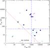 |
Fig. 16 Rotation period is plotted against the orbital period for the spectroscopic binaries for which these two periods are sufficiently constrained by the existing observations. Asterisks and crosses represent stars not known to have magnetically resolved lines, for which both periods were retrieved from the literature; crosses distinguish those for which uncertainties remain about some of the relevant parameters (see text). All other symbols correspond to Ap stars with magnetically resolved lines studied in detail in this paper. Dots identify those stars for which both periods are exactly known; open circles, stars with fully determined rotation periods for which only a lower limit of the orbital period has been obtained so far; filled triangles, stars with a known orbital period but only a lower limit of the rotation period; and open triangles, stars that have only been observed over a fraction of both their rotation and orbital periods. The short-dashed diagonal line represents the locus log Prot = 3.9−log Porb. The long-dashed horizontal line corresponds to Prot = 50 d and the long-dashed vertical line to Porb = 1000 d. |
For the systems appearing in Tables 18 and 19 for which both the rotation and orbital periods are constrained, we plot these two periods (or their lower limits) against each other in Fig. 16. Open symbols are used for stars for which only a lower limit of the orbital period could be obtained so far, while triangles identify lower limits of the rotation period. Asterisks and crosses represent stars not known to show magnetically resolved lines, for which the values of both periods were retrieved from the literature (that is, the stars listed in Table 19); among them, crosses distinguish the three stars discussed above, for which some of the relevant parameters are subject to uncertainties.
A striking feature of Fig. 16 is that all the stars with magnetically resolved lines are confined to the upper right region of the figure. To help visualise this, we plotted a dashed diagonal line defined by log Prot = 3.9−log Porb, which is approximately the lower envelope (both in Prot and in Porb) of the representative points of the stars studied in this paper.
Five of the stars of Table 19 also have representative points lying above or very near this dividing line. The main exceptions are HD 219749 and the four synchronised systems, HD 5550, HD 25267, HD 25823, and HD 98088, which appear in isolation in the lower left corner of the figure; the representative points of HD 25267 and HD 98088 are superimposed owing to the similarity of their periods.
The separation between two of the stars below and to the left of the diagonal line, HD 123335 and HD 191654, and the bulk of the sample, is much less clear cut. Indeed, a different way to look at the result illustrated in Fig. 16 is highlighted by the horizontal and vertical long-dashed lines drawn in this figure. The former corresponds the value 50 d of the stellar rotation period, the latter corresponds to a 1000-d long orbital period. Of the stars represented, only the four synchronised systems and HD 219749 are found in the lower left quadrant defined by these two lines. But for HD 219749, barring synchronisation, (relatively) short rotational, and orbital periods seem to be mutually exclusive. More specifically, in Fig. 16, 11 of the 12 non-synchronised spectroscopic binaries with a rotation period shorter than ~50 d have orbital periods in excess of 1000 d. Conversely, only 1 of the 12 non-synchronised spectroscopic binaries with an orbital period shorter than 1000 d has a rotation period shorter than ~50 d. On the other hand, a few stars have both a long rotation period and a long orbital period. Also keep in mind that stars represented by open symbols are bound to move further right in the diagram, while those appearing as triangles are due to raise further up when observations have been obtained over full periods.
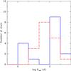 |
Fig. 17 Comparison between the distribution of the orbital periods of binaries containing an Ap star with a rotation period shorter (solid blue line) and greater (dashed red line) than 50 days. |
A different illustration of the systematics of the rotation and orbital periods of the stars of Tables 18 and 19 is shown in Fig. 17. The solid line histogram represents the distribution of the orbital periods of systems in which the Ap component has a rotation period shorter than 50 days. It is visibly different from the dashed line histogram, which corresponds to the orbital periods of the systems with an Ap component whose rotation period exceeds 50 days. To quantify this comparison, we have run a two-sided Kolmogorov-Smirnov test, which shows that the distribution of Porb in the two subsamples under consideration is different at the 89% confidence level. If we leave the three synchronised systems (the lower peak of the solid line histogram) out of the Prot < 50 d sample, the confidence level increases to 99.6%.
We can further test that the inferred deficiency of non-synchronised systems with both (relatively) short rotation and orbital periods is not the result of a chance coincidence through consideration of the projected equatorial velocity of the Ap component of systems with Porb < 1000 days, in some of the cases for which the rotation period of this component is not known. Such a test is meaningful only for those stars for which accurate determinations of v sini based on spectra of high enough resolution are available. Remember that for a star whose radius is 2 R⊙, and for which Prot = 10 d, v sini ≤ 10 km s-1, its value cannot be accurately determined from the analysis of low to moderate spectral resolution spectra and, hence, is not accurately constrained by the v sini data available in most catalogues.
In this context, the study of Carrier et al. (2002) contains the most extensive and homogeneous set of suitable v sini determinations. We briefly discuss the stars of this study with Porb < 1000 d that do not have a known rotation period; these are HD 22128, 54908, 56495, 73709, 105680, 138426, 188854, and 200405.
Four of these stars (HD 56495, 73709, 105680, and 188854) are classified as Am stars in the Renson & Manfroid (2009) catalogue. Carrier et al. (2002) acknowledge the ambiguity of their classification. Çakırlı (2015) recently reported that HD 188854 is an eclipsing binary whose primary is a γ Dor pulsating star; this makes it very unlikely that it is an Ap star. Bertaud & Floquet (1967) explicitly mentioned that they could not confirm the anomalous strength of the Sr lines in HD 105680 reported in the HD catalogue, and that they found its spectrum consistent with an Am classification. The Am nature of HD 73709 is confirmed by the detailed abundance analysis of Fossati et al. (2007), who also ruled out the presence of a detectable magnetic field in this star (which was suggested by Carrier et al.). In another detailed analysis, Folsom et al. (2013b) confirmed that HD 56495 is not an Ap star; furthermore, they also found both components of the SB2 system HD 22128 to be Am stars. While Renson & Manfroid (2009) give a spectral type A0p Si for HD 54908, we could not find this classification in the Bidelman & MacConnell (1973) work to which Carrier et al. (2002) refer, and the star is assigned spectral type A1m in the Michigan Catalogue (Houk & Swift 1999).
For HD 138426 ( ), v sini is small enough (≲2 km s-1) to be compatible with a rotation period of the order of 50 days or longer. For the remaining star, HD 200405 (
 ), the existing constraints are compatible with the synchronisation of the rotation of the Ap component with the orbital period. Indeed, assuming that the Ap component is rotating synchronously, hence that Prot = Porb = 1.635 d and that its radius is of the order of 2.4 R⊙, which should be fairly representative for the spectral type of interest, application of the relation
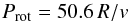 (25)yields v = 74 km s-1. Then v sini = 9.6 km s-1 implies that i ≃ 7.4°, which is consistent with the conclusion by Carrier et al. (2002) that the inclination of the orbital plane must be very small. The fact that the eccentricity of the orbit of HD 200405 is not significantly different from 0 further supports the plausibility that this systems is synchronous.
Thus, for the systems studied by Carrier et al. (2002) for which the Ap character of one of the components is unambiguously established, we did not find any definite indication that the relation between the rotation period of the Ap component and the orbital period of the system may not fit the pattern that we derived from consideration of the binaries containing Ap stars with known rotation periods.
This pattern is not questioned either by any of the spectroscopic binaries listed as Ap (including B9p and F0p) in the Pourbaix et al. (2004) catalogue. There are only four such stars that have not been already discussed above; these are HD 108945, HD 134759, HD 147869, and HD 196133. The binarity of HD 108945 cannot be regarded as confirmed. Consideration of Fig. 8 of Shorlin et al. (2002) and of Fig. 24 of Aurière et al. (2007) strongly suggests that the distortion of its line profiles resulting from abundance inhomogeneities on its surface must have mistakenly been interpreted as an SB2 signature by Abt & Willmarth (1999). The orbital period of HD 134759, 23.42 y (Heintz 1982), is much longer than 1000 d. It appears doubtful that HD 147869 and HD 196133 are actually Ap stars. Although HD 147869 is listed as an A1p Sr star by Renson & Manfroid (2009), it had been classified as A1 III by Abt & Morrell (1995); Lehmann et al. (2002) also regard it as an evolved star rather than a (chemically peculiar) main-sequence star. Renson & Manfroid (2009) note that HD 196133 is perhaps an Am star rather than an Ap star, while Bertaud & Floquet (1967) explicitly state that it is an A2 star without any noticeable peculiarity.
In summary, we have established the existence, with a high probability, of a connection between rotation and orbital periods for Ap stars in binaries. Namely, barring synchronisation, Ap components with short rotation periods (i.e. less than about 50 days) are found only in systems with very long orbital periods (more than 1000 days or so). Conversely, whenever a binary containing an Ap component has a short orbital period (that is, shorter than 1000 days), the rotation period of the Ap component is long (greater than 50 days). So far, this mutual exclusion of short rotational and orbital periods, as we shall refer to it from here on, suffers only one exception, HD 219749, for which Prot = 1.61 d and Porb = 48.30 d. HD 68351, if its suspected periods are confirmed, may formally represent another exception. However, this exception is at most marginal, since it would vanish if the cut-off line between short and long orbital periods, which involves a significant degree of arbitrariness, was shifted from the adopted value of 1000 days to 500–600 days.
We do not regard the HD 219749 exception as sufficient to question the reality of the mutual short period exclusion, since there is a realistic probability, in a sample of 29 systems, that one may have undergone some external disturbance altering its evolution. We are strengthened in this position by the fact that consideration of the available high-quality v sini information for the Ap component of additional systems, in which the rotation period of this component is unknown, did not indicate a definite inconsistency for any of these systems with the mutual exclusion of short rotational and orbital periods.
The lack of non-synchronised systems where both the rotational and orbital periods are short is unlikely to result from an observational bias. On the contrary, one might argue that long orbital periods are more likely to be overlooked in faster rotating stars, in which the achievable precision of radial velocity determinations is limited by the rotational Doppler broadening of the spectral lines.
Understanding the origin of the observed behaviour represents a challenge. There is no obvious physical mechanism to slow down the rotation of the Ap component of systems with orbital periods shorter than 1000 days. Tidal braking should be practically insignificant in the majority, if not all, of these systems because the shortest orbital period of the considered systems is 27 days, and all of the orbital periods, except for three, are longer than 100 days. As a matter of fact, in 9 of the 11 systems with Porb< 1000 d and Prot> 50 d from Tables 18 and 19, the rotation period of the Ap component is longer than the orbital period of the system: tidal interactions cannot account for the slow rotation of the Ap star.
With nothing in the present state of the systems apparently accounting for the mutual exclusion of short rotational and orbital periods, the explanation of the latter must be sought in the earlier evolution of these systems. Recently, two groups have, independently from each other, proposed a scenario for the origin of the magnetic fields of Ap stars in which these stars result from the merging of two lower mass stars or protostars (Ferrario et al. 2009; Tutukov & Fedorova 2010). In this scenario, the binaries that we observe now were triple systems earlier in their history. One can expect such a dynamical event as the merger of two of the three components of a triple system not only to determine the rotation rate of the resulting merged star, but also to have a significant impact on the orbit of the third component. Thus the merging scenario for the origin of Ap stars provides a plausible link between the rotational period of the Ap component of binary sytems and their orbital period. Conversely, the mere existence of a connection between rotational and orbital periods in Ap binaries represents a very strong argument in support of the merging scenario for the origin of Ap stars. The details of the merging process are complex, and their study is beyond the scope of this paper. The observational results reported here should represent useful constraints for its theoretical modelling.
The merging scenario is consistent with the recent identification of a group of magnetic Herbig Ae/Be stars as the likely progenitors of the main-sequence Ap stars (e.g. Alecian et al. 2013a; Hubrig et al. 2009b, and references therein) as long as the merger is completed early enough at the pre-main-sequence stage for its result to appear as a Herbig Ae/Be star. Ferrario et al. (2009) explicitly stress that one (at least) of the merging stars must be on the Henyey part of the pre-main-sequence track towards the end of its contraction to the main sequence. This makes it very plausible that the outcome becomes observable as a Herbig Ae/Be star. Once the merger is completed, the stellar field should then be essentially indistinguishable from the fossil fields hypothesised by the more traditional theories of the origin of Ap star magnetism. Furthermore, since the angular momentum is shed out during the merging process, no further rotational braking is needed at either the pre-main-sequence or main-sequence stage, which is consistent with the observation that Herbig Ae/Be stars achieve slow rotation at an extremely early phase (Alecian et al. 2013b).
How the synchronised binaries fit in the merging scenario is not entirely clear. In such a binary, the initial rotation period of the Ap component at the end of its formation must have been shorter than the orbital period of the system (so that, with time, tidal braking would synchronise it). By contrast, if we are correct in our interpretation that the connection between rotational and orbital periods is due to the formation of the Ap component through merging, the long rotation period of the Ap component of binaries with short orbital periods (that is, the systems in the upper left quadrant of Fig. 16) must have been defined at the time when they formed from the merger of two lower mass stars. Thus we have two very different populations of Ap stars in binaries: one with stars that had initial rotation periods not exceeding a few days, and the other whose members have had rotation periods longer than ~50 days since the time of their formation.
Synchronised binaries may be systems whose components were originally close enough to develop an interaction leading to the generation of a magnetic field in one of the stars, but not to lead to merging. The field then allowed chemical peculiarities to develop in the magnetic component, which became an Ap star without merging. Alternatively, it is very possible that Ap stars in synchronised binaries formed through a completely different channel. As stressed by Tutukov & Fedorova (2010), even if merging is the main channel of formation of Ap stars, this does not rule out the possibility that some are formed through other processes.
Within this picture, there are various plausible paths leading to the exception of HD 219749, the only non-synchronised binary known so far with a (relatively) short orbital period (48 days) and an Ap component with a short rotation period (1.6 day). HD 219749 may have formed through the merger scenario as a single Ap star with a short rotation period, and it may have acquired a companion later in its evolution through a chance encounter. Or this binary may have originally been a triple system, of which two components merged to form an Ap star with a distant companion, with an orbital period greater than 1000 days. In such a binary, the Ap component could have a short rotation period. This binary would then have undergone some external perturbation later in its life, leading to its components getting closer to each other with a considerably shortened orbital period. A third possibility is that the system formed through the synchronised binary channel, rather than the merger channel, and that an external perturbation later in its life led to its components moving further apart, with an increased orbital period. Thus, as already mentioned, the exception of HD 219749 does not question the general conclusion that, as a rule, short orbital and rotational periods are mutually exclusive in non-synchronised systems.
6. Conclusions
We carried out the most exhaustive statistical study to date of a sample of Ap stars with magnetically resolved lines. It is based on extensive sets of previously unpublished measurements of various parameters characterising them:
-
Measurements of their mean magnetic field modulus at differentepochs. These measurements complement those presented inPaper I for 40 of these stars, considerablyextending the time span that they covered.
-
Multi-epoch determinations from spectropolarimetric observations of their lowest order field moments: mean longitudinal magnetic field, crossover, and mean quadratic field. For about a quarter of the studied stars, our data represent the first ever determinations of these field moments. For many others, only very few such measurements had been obtained before, in most cases sparsely sampling the rotation cycles of the considered stars, hence unsuitable to constrain their variability. Improved phase sampling and extended time span coverage result from the combination of the new measurements of this paper with those of our previous studies (Mathys 1994, 1995a,b; Mathys & Hubrig 1997; note also the revised quadratic field values of Appendix B), allowing many variation curves to be defined for the first time.
-
Radial velocity determinations from almost all the observations of Mathys (1991), Mathys & Hubrig (1997), Paper I, and the present study.
Whenever appropriate, we complemented the measurements detailed above with similar data from the literature. We exerted great care in the selection of the latter, to ensure as much as possible that they were of similar (or better) quality and reliability as our own data. There was little concern in that respect for mean magnetic field modulus determinations from other authors. But our critical evaluation of the published determinations of other parameters revealed a much wider range in their suitability for our purposes. In particular, many ambiguities were found with respect to the peculiarity class (Ap or Am, or even non-peculiar) of a number of stars, to their rotation and orbital periods, or even to their binarity.
Analysis of these data enabled us to confirm and refine the results established in Paper I with increased significance, reveal the existence of additional statistical trends, and present supporting evidence for the occurrence of physical processes that were little studied until now. Hereafter, we summarise these results, we consider possible ways of submitting them to additional tests, and we discuss their implications for our general understanding of the Ap stars and their magnetic fields.
Neither our new mean magnetic field modulus data, nor the much less extensive measurements of this field moment in the large number of additional Ap stars with resolved magnetically split lines whose discovery was reported in the literature in recent years, call into question the existence of a sharp discontinuity at the low end of the ⟨ B ⟩ distribution. The location of this discontinuity, about 2.8 kG (in terms of average of the field modulus over the stellar rotation cycle), is confirmed. The observations presented in this paper also strengthen the arguments developed in Paper I against the possibility that this discontinuity is only the apparent consequence of observational limitations.
A number of detections of magnetic fields below the magnetic resolution threshold through modelling of differential broadening of lines of different magnetic sensitivities were published in the meantime, all yielding field strengths not exceeding 1.5 kG. Thus, while based on the results presented in Paper I, one could speculate the existence of a cut-off at the low end of the field intensity distribution, a much more intriguing picture now seems to emerge, in which the distribution of the magnetic field strengths of the slowly rotating Ap stars is bimodal, with a narrow peak below ~2 kG and a broad, spread out distribution above approximately 2.8 kG, separated from each other by a gap in which no star is found.
The reality of the existence of this gap should be further tested. Its boundaries should be better established, especially on the low field side. The rate of occurrence and distribution of field strengths below 2 kG should be studied. Whether the bimodal distribution of the field strengths is specific to the slowly rotating Ap stars or whether it extends to their faster rotating counterparts also needs to be investigated.
Those stars that show (or may show) magnetically resolved lines only for part of their rotation cycle are especially interesting, and they deserve to be followed throughout their whole period. This is needed in particular to confirm our suspicion that in stars where the line Fe iiλ 6149.2 is magnetically resolved at some phases, the average over the rotation cycle of the mean field modulus is always greater than or equal to ~ 2.8 kG.
It is almost impossible for it to be significantly lower in HD 9996, as ⟨ B ⟩ reaches ~5.1 kG at its maximum and the observed shape of its variation around the latter (Fig. A.4) indicates that it must exceed 3 kG over nearly half the rotation period of the star. In HD 18078, the phase interval over which the Fe iiλ 6149.2 line is not resolved is too narrow for the value ⟨ B ⟩ av = 3.45 kG, which is derived by fitting the ⟨ B ⟩ measurements over the rest of the cycle to be much greater than the actual average value of the mean field modulus over the whole rotation period. The star that may be best suited for a critical test of the ⟨ B ⟩ av lower limit is HD 184471, provided that our suspicion that Fe iiλ 6149.2 can be resolved into its split components over part of its rotation cycle (see Sect. 5.6) is correct. Furthermore, its fairly short rotation period,  , lends itself well to achieving good phase coverage of its field modulus variation curve in a reasonable time.
On the low side of the conjectured ⟨ B ⟩ distribution gap, as part of our systematic search for Ap stars with magnetically resolved lines, we identified a significant number of (very) low v sini Ap stars with unresolved lines. Systematic determination of their magnetic fields, or upper limits thereof, from the analysis of differential broadening of lines of different magnetic sensitivities, will allow us to probe the low end of the ⟨ B ⟩ distribution. However, the rotation period of the vast majority of these stars is unknown. It is likely long for most of them and its determination may not be straightforward. Photometry has proved poorly suited to studying variations on timescales of months or years. Spectral line profile variations in natural light may be small and difficult to analyse as magnetic broadening is not the dominant contributor to the overall line width. Studying the variability of the mean longitudinal magnetic field appears to be the most effective approach to constrain the rotation periods of the sharp-lined Ap stars whose lines are not resolved into their magnetically split components. In any event, characterisation of the distribution of the magnetic field strengths of Ap stars below 1.5–2.0 kG will require a significant, long-term effort.
Here we confirm, refine, and complement our previously established dependencies of the magnetic field strength and structure on the rotation period (Paper I; Landstreet & Mathys 2000; Bagnulo et al. 2002).
The conclusion from Paper I that very strong magnetic fields (⟨ B ⟩ av> 7.5 kG) occur only in stars with rotation periods of less than ~150 days was strengthened by the larger size of the sample of stars on which it is based (in part thanks to the inclusion of additional stars from the literature) as well as by the increase in significance of the values of ⟨ B ⟩ av resulting from the improved phase coverage of the measurements for many of the studied stars. In order to further test it, one should focus first on determining the rotation periods of those stars most likely to have ⟨ B ⟩ av> 7.5 kG for which their values have not yet been derived and for which v sini is small; these stars are HD 47103 and HD 66318 (see Sect. 5.1).
Continued observation of the stars for which the data available so far do not fully constrain the mean field modulus variation curve will make the set of ⟨ B ⟩ av values increasingly representative of the actual stellar field strengths. This pending improvement will be particularly important for the stars whose rotation period is longer than the time frame spanned by the measurements performed up to now. For the majority of these stars, the actual value of ⟨ B ⟩ av may be somewhat greater than the current estimate based on data sampling only a fraction of the period, if the tendency of the ⟨ B ⟩ variation curves of the slowest rotating stars to have broad, nearly flat bottoms advocated in Sect. 5.1 is confirmed. This putative systematic increase of ⟨ B ⟩ av for the slowest rotators is however very unlikely to be sufficient to question or significantly alter the above-mentioned conclusion about the lack of very strong magnetic fields in the long-period Ap stars. However, it will be interesting to confirm if the apparent tendency for very slowly rotating stars to show in general higher values of the ratio q between the extrema of the field modulus (Fig. 4) is strengthened as the fraction of their period over which ⟨ B ⟩ measurements were obtained increases. An open question is whether q may in some cases be much greater than 2.
Landstreet & Mathys (2000) and Bagnulo et al. (2002) mostly used the values of the magnetic moments presented here for those stars for which full coverage of the rotation cycle is achieved to reach the conclusion that the angle between the rotation and magnetic axes is generally large in stars with rotation periods shorter than 1–3 months, while these axes tend to be aligned in slower rotating stars. The longest period stars are omitted from those studies. Nevertheless, even though the data presented here for the slowest rotators do not completely sample the field variations, they are useful to complement the results of the above-mentioned works and to amend their conclusions. Their indication that for Prot ≳ 1000 d, large β angles become predominant again appears convincing.
The point that remains more debatable at this stage is whether near alignment of the magnetic and rotation axes actually occurs in an intermediate period range (approximately 100–1000 d), or whether this apparent trend is just coincidental, resulting from the insufficient population of the sample of stars that could be studied in that range. Hopefully, that population will grow once the rotation periods of the stars with magnetically resolved lines that have so far only been observed at few epochs (that is, primarily, most stars of Table 2) have been determined. At present, there are two stars with periods in that range for which the existing data are insufficient to constrain the magnetic field geometry; these are HD 110274 (which has magnetically resolved lines) and HD 221568 (which does not). Systematic measurements of their mean longitudinal magnetic fields, and of the mean magnetic field modulus of HD 110274, throughout their rotation cycles, will valuably complement our current knowledge of the field properties in the 100–1000 d Prot range.
One of the particularly interesting outcomes of this study is the identification of a small number of stars showing considerable deviations with respect to the statistical trends that apply to the bulk of the studied sample and, hence, presumably to the majority of Ap stars with moderate or slow rotation. Remarkably, the exceptions comprise some of the most famous and best-studied Ap stars, i.e. HD 65339, HD 137909, HD 215441. On the one hand, it is very fortunate that these stars have been extensively studied for several decades, since the consideration of exceptions and extreme cases often provide especially valuable clues towards the understanding of the physical processes that are at play in the type of objects to which they belong. This represents a strong incentive to continue to study them in ever greater detail. On the other hand, these outliers should not be regarded as representative or typical of the common properties or general behaviour of magnetic Ap stars: one should be cautious not to generalise the conclusions drawn about them to the class as a whole – this is a mistake that has occasionally been made in the past.
Other, less studied stars that prove to be atypical in some respects include HD 18078, HD 51684, HD 93507, HD 94660, and HD 126515. All deserve additional investigation, as understanding what makes their magnetic fields different from the majority may also provide important clues about the physical processes at play for the latter.
The better quality and coverage of the new spectropolarimetric observations analysed here, compared to those of our previous studies, and the resulting improvement in the precision of the magnetic field moments that we derived from them, have enabled us to achieve significant measurements of rotational crossover in longer period stars. That is not unexpected, but a more intriguing result is the apparent detection of crossover in stars whose rotation is definitely too slow to generate the Doppler line shifts required to account for that effect. Those detections are, however, close to the limit of formal significance, and while we have presented various arguments to support their reality, they beg for further confirmation.
The most straightforward way to obtain such confirmation will be to try to reproduce the detections achieved here for new, similar observations of the same stars. The higher resolution, broader spectral coverage and better stability of modern spectropolarimeters such as ESPADONS or HARPSpol should ensure that much more precise determinations of the crossover should be achievable. With lower uncertainties, crossover values of the order reported here should be measurable at a sufficient level of significance to dispel any doubt about their reality.
If that endeavour is successful, the next step will be to test the interpretation that we proposed, that pulsation is responsible for that new type of crossover. In that case, the crossover should vary with the pulsation frequency; this can be probed by acquiring spectropolarimetric observations with a time resolution that is shorter than the pulsation period, similar to the high time and spectral resolution observations that have been used to study pulsation-induced line profile variations (e.g. Elkin et al. 2008).
Admittedly, among the stars in which we detect a formally significant crossover that does not appear to be of rotational origin, only HD 116114 is known to be pulsating. This makes it a prime candidate for the considered observational test, all the more since it has one of the longest pulsation periods known among roAp stars (Elkin et al. 2005b), such that it is particularly well suited to obtaining pulsation-phase-resolved spectropolarimetric observations; it is also relatively bright.
However that should not detract one from attempting a similar experiment for some of the other stars in which crossover that cannot be accounted for by rotation has apparently been detected (see Sect. 5.3). It should be reasonable to assume that, if they pulsate at all, they do so at frequencies similar to those of the known roAp stars, and to obtain observations with a matching time resolution. Those observations would then probe the occurrence of pulsations that cannot be detected photometrically or via studies of radial velocity and line profile variations, possibly because they correspond to non-radial modes of high degree ℓ. Such success would open the door to a whole new region of the parameter space in asteroseismological studies of Ap stars.
Our long-term monitoring of the magnetic variations of Ap stars with resolved magnetically split lines has allowed us to set new constraints on many rotation periods. A significant number of stars proved to rotate so slowly that even observations spanning time intervals of several years – in some cases, more than a decade – fall very short of covering a full cycle. The resulting increase in the number of Ap stars known to have extremely long periods led to the realisation of the existence of a considerable population of Ap stars that rotate extremely slowly. Stars with periods in excess of one year must represent several percent of all Ap stars.
The long-period tail of the distribution of the rotation periods of Ap stars is now sufficiently populated to allow statistical inferences to be drawn. The most definite one at this stage is the first concrete evidence that some of the rotation periods must be as long as 300 yr. The existence of such long periods makes it absolutely essential to continue to monitor the variations of the corresponding stars. It makes us responsible to future generations of researchers; any gaps that we may leave today in the phase coverage of the variations of those super-slow rotators may not be recoverable for decades or centuries. Such gaps may heavily hamper scientific progress by making it impossible to fully characterise the properties of the longest period stars and to identify possible differences between them and faster (or less slow) rotators.
The impact is not restricted to the knowledge of the slowest rotators; it also extends to our general understanding of the Ap phenomenon. The 5 to 6 orders of magnitude spanned by their rotation periods represent a unique property that distinguishes them from all other stellar types. Since the evolution of their rotation rates during their lifetimes on the main sequence are mostly consistent with conservation of the angular momentum, the definition of those rates must be a fundamental part of the stellar formation and early evolution processes. Knowledge of the longest periods and the other stellar properties with which they are correlated must therefore be one of the keys to the unravelling of those processes.
On the other hand, the knowledge acquired about the long-period tail of the distribution of the rotation periods of Ap stars so far is mostly restricted to the strongly magnetic members of that class (that is, in practice, stars with ⟨ B ⟩ av ≳ 2.8 kG). As mentioned in Sect. 5.5, of the 36 stars with Prot> 30 d currently known, only 4 do not show magnetically resolved lines. But there must also exist a sizeable population of weakly magnetic stars that rotate very slowly. We need to identify and to study them to obtain a complete picture of super-slow rotation in Ap stars and to gain further insight into the processes at play during their formation and early evolution that lead to the huge spread in their rotation velocities by the time when they arrive on the main sequence. Observationally, this undertaking overlaps with the above-mentioned study of the distribution of the magnetic field strengths of Ap stars below 1.5–2.0 kG.
The significance of rotation for the understanding of the Ap phenomenon is further emphasised by the unexpected discovery of correlations between the rotation periods of Ap components of binaries and the orbital periods of those systems. It is highly significant that the orbital period is not shorter than 27 days for any of the binaries in which the Ap component has magnetically resolved lines. It is a very solid result because the probability that a short-period spectroscopic binary may have been overlooked by our intensive monitoring is vanishingly small. This could have happened only for very rare combinations of an orbital plane seen very nearly face-on and a very low mass secondary. Even if a couple of such systems had been overlooked, the general conclusion that there is a deficiency of binaries with short orbital periods among systems containing an Ap star with resolved magnetically split lines would still remain valid.
Actually, among Ap stars in binaries that do not show magnetically resolved lines for which both the rotation and the orbital periods are known (see Table 19), there is also a deficiency of orbital periods shorter than 27 days: only the three synchronised systems have such periods. All others, except for HD 219749, have either Porb> 1000 d, or Prot> 50 d in combination with a magnetic field too weak for their spectral lines to be observationally resolved into their split components.
That lack of known non-synchronised systems in which both the rotation and orbital periods are short for Ap stars that do not show magnetically resolved lines as well as for those that do show them led us to the conclusion that, for Ap stars in binaries, barring synchronism, short rotation periods and short orbital periods are mutually exclusive. This result begs further confirmation, even though it is established at a high level of statistical significance from the most complete sample that we could build by combining our new data with all the relevant information of sufficient quality that we could find in the literature.
The acid test consists of trying to find Ap stars with rotation periods shorter than 50 days in non-synchronised binaries with orbital periods shorter than 1000 days. To this effect, it is critical to confirm the peculiarity of the presumed Ap component of those binaries. Indeed, we found in Sect. 5.6 that in a surprisingly large number of the systems that have in the past been considered as Ap binaries, that classification appears to be definitely or very probably mistaken. Accordingly, there remain only very few binaries that have a reliably known orbital period shorter than 1000 days and contain an Ap component whose rotation period has not been determined. We have been able to identify only two such systems; these are HD 138426 and HD 200405. An observational effort should be undertaken to study the variability of their Ap components.
More generally, taking into account the classification inaccuracies that appear to have plagued previous studies, it is worth reconsidering the distribution of the orbital periods of the binaries containing Ap components. The exhaustive BinaMIcS project is already revisiting its short-period tail in a systematic manner and the (still partial) results obtained until now unambiguously show it to be significantly less populated than previously thought (Alecian et al. 2015). On the other hand, while the nature of our study of the magnetic fields of the Ap stars with resolved magnetically split lines has also made it particularly appropriate for the discovery and characterisation of long-period spectroscopic binaries, complementing the knowledge of that population with systems containing faster-rotating Ap components may prove much more elusive.
We argued in Sect. 5.6 that the existence of a connection between the rotation and orbital periods of Ap stars in binaries represents a strong argument in favour of a merger scenario for their formation. Many of the other results presented in this paper, including those about the distributions of the rotation periods of the Ap stars and of the strengths of their magnetic fields, and about the correlation between rotation and magnetic properties, are products of the evolution process that they have undergone. Taken together, those various elements must guide the theoretical developments aimed at explaining the origin of magnetism in a fraction of the main-sequence stars of spectral type A and possibly also of hotter stars. This remains one of the least well-understood aspects of stellar physics, in which hopefully our contribution will enable significant progress to be achieved. As discussed in the present section, this contribution does not represent the final word on the observational side, as some of its conclusions beg for further confirmation, and even more, as it raises a number of additional, sometimes unexpected, questions. We have highlighted some of these questions and proposed ways to address them, tracing a possible path for continued investigation of some of the most intriguing and potentially enlightening aspects of the magnetism of Ap stars.
However, the Babcock (1960) observations of HD 215441, on which his discovery of magnetically resolved lines was based, were obtained in October 1959. HD 126515 (also known as Preston’s star) actually appears to be the first star for which spectra showing magnetically resolved lines were recorded, in February 1957 – as Preston (1970) found later, motivated by a remark made by Babcock (1958) on the unusual appearance of the line profiles.
The older data from Mathys (1995a) and Mathys & Hubrig (1997) are not considered in this part of the discussion because of their lower precision.
Acknowledgments
A large portion of this study has been carried out during stays of the author in the Department Physics and Astronomy of the University of Western Ontario (London, Ontario, Canada). I thank John Landstreet for giving me the opportunity of these visits and for providing partial funding to support them. Financial support received from the ESO Director General’s Discretionary Fund (DGDF) also contributed to make these stays possible. I am grateful to Swetlana Hubrig, John Landstreet, Jean Manfroid, and Gregg Wade, for their participation in the excution of some of the observations, and to Steven Arenburg, Jean Manfroid, and Erich Wenderoth for their contributions to their initial reduction; Wenderoth’s participation in the project was also funded by the ESO DGDF. This research has made use of the SIMBAD database, operated at the CDS, Strasbourg, France
References
- Abt, H. A., & Morrell, N. I. 1995, ApJS, 99, 135 [Google Scholar]
- Abt, H. A., & Snowden, M. S. 1973, ApJS, 25, 137 [NASA ADS] [CrossRef] [Google Scholar]
- Abt, H. A., & Willmarth, D. W. 1999, ApJ, 521, 682 [NASA ADS] [CrossRef] [Google Scholar]
- Adelman, S. J. 1981, A&AS, 44, 265 [NASA ADS] [Google Scholar]
- Adelman, S. J. 1989, MNRAS, 239, 487 [NASA ADS] [CrossRef] [Google Scholar]
- Adelman, S. J. 1997, PASP, 109, 9 [NASA ADS] [CrossRef] [Google Scholar]
- Adelman, S. J. 2000a, A&AS, 146, 13 [NASA ADS] [CrossRef] [EDP Sciences] [Google Scholar]
- Adelman, S. J. 2000b, A&A, 357, 548 [NASA ADS] [Google Scholar]
- Adelman, S. J. 2001, A&A, 368, 225 [Google Scholar]
- Adelman, S. J. 2006, PASP, 118, 77 [NASA ADS] [CrossRef] [Google Scholar]
- Adelman, S. J., & Boyce, P. W. 1995, A&AS, 114, 253 [NASA ADS] [Google Scholar]
- Alecian, E., Neiner, C., Wade, G. A., et al. 2015, in New Windows on Massive Stars, eds. G. Meynet, C. Georgy, J. Groh, & P. Stee, IAU Symp., 307, 330 [Google Scholar]
- Alecian, E., Tkachenko, A., Neiner, C., Folsom, C. P., & Leroy, B. 2016, A&A, 589, A47 [NASA ADS] [CrossRef] [EDP Sciences] [Google Scholar]
- Alecian, E., Wade, G. A., Catala, C., et al. 2013a, MNRAS, 429, 1001 [NASA ADS] [CrossRef] [Google Scholar]
- Alecian, E., Wade, G. A., Catala, C., et al. 2013b, MNRAS, 429, 1027 [NASA ADS] [CrossRef] [Google Scholar]
- Alentiev, D., Kochukhov, O., Ryabchikova, T., et al. 2012, MNRAS, 421, L82 [NASA ADS] [Google Scholar]
- Aurière, M., Wade, G. A., Silvester, J., et al. 2007, A&A, 475, 1053 [NASA ADS] [CrossRef] [EDP Sciences] [Google Scholar]
- Babcock, H. W. 1954, ApJ, 120, 66 [NASA ADS] [CrossRef] [Google Scholar]
- Babcock, H. W. 1958, ApJS, 3, 141 [NASA ADS] [CrossRef] [Google Scholar]
- Babcock, H. W. 1960, ApJ, 132, 521 [NASA ADS] [CrossRef] [Google Scholar]
- Babel, J., & North, P. 1997, A&A, 325, 195 [NASA ADS] [Google Scholar]
- Babel, J., North, P., & Queloz, D. 1995, A&A, 303, L5 [NASA ADS] [Google Scholar]
- Bagnulo, S., Landolfi, M., Mathys, G., &Landi Degl’Innocenti, M. 2000, A&A, 358, 929 [NASA ADS] [Google Scholar]
- Bagnulo, S., Wade, G. A., Donati, J.-F., et al. 2001, A&A, 369, 889 [NASA ADS] [CrossRef] [EDP Sciences] [Google Scholar]
- Bagnulo, S., Landi Degl’Innocenti, M., Landolfi, M., & Mathys, G. 2002, A&A, 394, 1023 [NASA ADS] [CrossRef] [EDP Sciences] [Google Scholar]
- Bagnulo, S., Landstreet, J. D., Lo Curto, G., Szeifert, T., & Wade, G. A. 2003, A&A, 403, 645 [NASA ADS] [CrossRef] [EDP Sciences] [Google Scholar]
- Bagnulo, S., Landstreet, J. D., Mason, E., et al. 2006, A&A, 450, 777 [NASA ADS] [CrossRef] [EDP Sciences] [Google Scholar]
- Bagnulo, S., Fossati, L., Landstreet, J. D., & Izzo, C. 2015, A&A, 583, A115 [NASA ADS] [CrossRef] [EDP Sciences] [Google Scholar]
- Bailey, J. D., Landstreet, J. D., Bagnulo, S., et al. 2011, A&A, 535, A25 [NASA ADS] [CrossRef] [EDP Sciences] [Google Scholar]
- Bailey, J. D., Grunhut, J., & Landstreet, J. D. 2015, A&A, 575, A115 [NASA ADS] [CrossRef] [EDP Sciences] [Google Scholar]
- Belopolsky, A. 1913, Astron. Nachr., 195, 159 [NASA ADS] [CrossRef] [Google Scholar]
- Bertaud, C., & Floquet, M. 1967, J. Observateurs, 50, 425 [Google Scholar]
- Bidelman, W. P., & MacConnell, D. J. 1973, AJ, 78, 687 [NASA ADS] [CrossRef] [Google Scholar]
- Bohlender, D. A., Landstreet, J. D., & Thompson, I. B. 1993, A&A, 269, 355 [NASA ADS] [CrossRef] [Google Scholar]
- Bonsack, W. K. 1976, ApJ, 209, 160 [NASA ADS] [CrossRef] [Google Scholar]
- Borra, E. F., & Landstreet, J. D. 1978, ApJ, 222, 226 [NASA ADS] [CrossRef] [Google Scholar]
- Borra, E. F., & Landstreet, J. D. 1980, ApJS, 42, 421 [NASA ADS] [CrossRef] [Google Scholar]
- Bychkov, V. D., Gerth, E., Kroll, R., & Shtol’, V. G. 1997, in Stellar Magnetic Fields, eds. Y. Glagolevskij, & I. Romanyuk, 204 [Google Scholar]
- Bychkov, V. D., Bychkova, L. V., & Madej, J. 2003, A&A, 407, 631 [NASA ADS] [CrossRef] [EDP Sciences] [Google Scholar]
- Bychkov, V. D., Bychkova, L. V., & Madej, J. 2006, MNRAS, 365, 585 [NASA ADS] [CrossRef] [Google Scholar]
- Bychkov, V. D., Bychkova, L. V., Madej, J., & Shatilov, A. V. 2012, Acta Astron., 62, 297 [NASA ADS] [Google Scholar]
- Bychkov, V. D., Bychkova, L. V., & Madej, J. 2016, MNRAS, 455, 2567 [NASA ADS] [CrossRef] [Google Scholar]
- Çakırlı, Ö. 2015, New Astron., 38, 55 [NASA ADS] [CrossRef] [Google Scholar]
- Carrier, F., North, P., Udry, S., & Babel, J. 2002, A&A, 394, 151 [NASA ADS] [CrossRef] [EDP Sciences] [Google Scholar]
- Catalano, F. A., & Renson, P. 1998, A&AS, 127, 421 [NASA ADS] [CrossRef] [EDP Sciences] [Google Scholar]
- Cowley, C. R., Bidelman, W. P., Hubrig, S., Mathys, G., & Bord, D. J. 2004, A&A, 419, 1087 [NASA ADS] [CrossRef] [EDP Sciences] [Google Scholar]
- Cowley, C. R., & Hubrig, S. 2008, MNRAS, 384, 1588 [NASA ADS] [CrossRef] [Google Scholar]
- Cowley, C. R., Hubrig, S., Ryabchikova, T. A., et al. 2001, A&A, 367, 939 [NASA ADS] [CrossRef] [EDP Sciences] [Google Scholar]
- Cunha, M. S. 2002, MNRAS, 333, 47 [NASA ADS] [CrossRef] [Google Scholar]
- Drummond, J., Milster, S., Ryan, P., & Roberts, Jr., L. C. 2003, ApJ, 585, 1007 [NASA ADS] [CrossRef] [Google Scholar]
- Dworetsky, M. M. 1982, The Observatory, 102, 138 [NASA ADS] [Google Scholar]
- Elkin, V. G., & Wade, G. A. 1997, in Stellar Magnetic Fields, eds. Y. Glagolevskij, & I. Romanyuk, 106 [Google Scholar]
- Elkin, V. G., Kurtz, D. W., Mathys, G., et al. 2005a, MNRAS, 358, 1100 [NASA ADS] [CrossRef] [Google Scholar]
- Elkin, V. G., Riley, J. D., Cunha, M. S., Kurtz, D. W., & Mathys, G. 2005b, MNRAS, 358, 665 [NASA ADS] [CrossRef] [Google Scholar]
- Elkin, V., Kurtz, D. W., & Mathys, G. 2008, Contributions of the Astronomical Observatory Skalnate Pleso, 38, 317 [NASA ADS] [Google Scholar]
- Elkin, V. G., Kurtz, D. W., Mathys, G., & Freyhammer, L. M. 2010a, MNRAS, 404, L104 [NASA ADS] [CrossRef] [Google Scholar]
- Elkin, V. G., Kurtz, D. W., Nitschelm, C., & Unda-Sanzana, E. 2010b, MNRAS, 401, L44 [NASA ADS] [CrossRef] [Google Scholar]
- Elkin, V. G., Mathys, G., Kurtz, D. W., Hubrig, S., & Freyhammer, L. M. 2010c, MNRAS, 402, 1883 [NASA ADS] [CrossRef] [Google Scholar]
- Elkin, V. G., Kurtz, D. W., & Mathys, G. 2011, MNRAS, 415, 2233 [NASA ADS] [CrossRef] [Google Scholar]
- Elkin, V. G., Kurtz, D. W., & Nitschelm, C. 2012, MNRAS, 420, 2727 [NASA ADS] [CrossRef] [Google Scholar]
- Ferrario, L., Pringle, J. E., Tout, C. A., & Wickramasinghe, D. T. 2009, MNRAS, 400, L71 [NASA ADS] [CrossRef] [Google Scholar]
- Floquet, M. 1977, A&AS, 30, 27 [NASA ADS] [Google Scholar]
- Folsom, C. P., Likuski, K., Wade, G. A., et al. 2013a, MNRAS, 431, 1513 [NASA ADS] [CrossRef] [Google Scholar]
- Folsom, C. P., Wade, G. A., & Johnson, N. M. 2013b, MNRAS, 433, 3336 [NASA ADS] [CrossRef] [Google Scholar]
- Fossati, L., Bagnulo, S., Monier, R., et al. 2007, A&A, 476, 911 [NASA ADS] [CrossRef] [EDP Sciences] [Google Scholar]
- Freyhammer, L. M., Elkin, V. G., Kurtz, D. W., Mathys, G., & Martinez, P. 2008, MNRAS, 389, 441 [NASA ADS] [CrossRef] [Google Scholar]
- Gerbaldi, M., Floquet, M., & Hauck, B. 1985, A&A, 146, 341 [NASA ADS] [Google Scholar]
- Hatzes, A. P., & Mkrtichian, D. E. 2004, MNRAS, 351, 663 [NASA ADS] [CrossRef] [Google Scholar]
- Heintz, W. D. 1982, A&AS, 47, 569 [NASA ADS] [Google Scholar]
- Hensberge, H., Nitschelm, C., Olsen, E. H., et al. 2007, MNRAS, 379, 349 [NASA ADS] [CrossRef] [Google Scholar]
- Hildebrandt, G., Scholz, G., & Lehmann, H. 2000, Astron. Nachr., 321, 115 [Google Scholar]
- Hill, G. M., Bohlender, D. A., Landstreet, J. D., et al. 1998, MNRAS, 297, 236 [NASA ADS] [CrossRef] [Google Scholar]
- Hockey, M. S. 1969, MNRAS, 142, 543 [NASA ADS] [CrossRef] [Google Scholar]
- Houk, N., & Swift, C. 1999, Michigan catalogue of two-dimensional spectral types for the HD Stars, 5 [Google Scholar]
- Hubrig, S., & Nesvacil, N. 2007, MNRAS, 378, L16 [NASA ADS] [CrossRef] [Google Scholar]
- Hubrig, S., North, P., & Mathys, G. 2000, ApJ, 539, 352 [NASA ADS] [CrossRef] [Google Scholar]
- Hubrig, S., Cowley, C. R., Bagnulo, S., et al. 2002, in Exotic Stars as Challenges to Evolution, eds. C. A. Tout, & W. van Hamme, ASP Conf. Ser., 279, 365 [Google Scholar]
- Hubrig, S., Kurtz, D. W., Bagnulo, S., et al. 2004a, A&A, 415, 661 [NASA ADS] [CrossRef] [EDP Sciences] [Google Scholar]
- Hubrig, S., Szeifert, T., Schöller, M., Mathys, G., & Kurtz, D. W. 2004b, A&A, 415, 685 [NASA ADS] [CrossRef] [EDP Sciences] [Google Scholar]
- Hubrig, S., Nesvacil, N., Schöller, M., et al. 2005, A&A, 440, L37 [NASA ADS] [CrossRef] [EDP Sciences] [Google Scholar]
- Hubrig, S., North, P., Schöller, M., & Mathys, G. 2006, Astron. Nachr., 327, 289 [NASA ADS] [CrossRef] [Google Scholar]
- Hubrig, S., Mathys, G., Kurtz, D. W., et al. 2009a, MNRAS, 396, 1018 [NASA ADS] [CrossRef] [Google Scholar]
- Hubrig, S., Stelzer, B., Schöller, M., et al. 2009b, A&A, 502, 283 [NASA ADS] [CrossRef] [EDP Sciences] [Google Scholar]
- Joshi, S., Mary, D. L., Chakradhari, N. K., Tiwari, S. K., & Billaud, C. 2009, A&A, 507, 1763 [NASA ADS] [CrossRef] [EDP Sciences] [Google Scholar]
- Kochukhov, O. 2003, A&A, 404, 669 [NASA ADS] [CrossRef] [EDP Sciences] [Google Scholar]
- Kochukhov, O., Landstreet, J. D., Ryabchikova, T., Weiss, W. W., & Kupka, F. 2002, MNRAS, 337, L1 [NASA ADS] [CrossRef] [Google Scholar]
- Kochukhov, O., Bagnulo, S., Wade, G. A., et al. 2004, A&A, 414, 613 [NASA ADS] [CrossRef] [EDP Sciences] [Google Scholar]
- Kochukhov, O., Tsymbal, V., Ryabchikova, T., Makaganyk, V., & Bagnulo, S. 2006, A&A, 460, 831 [NASA ADS] [CrossRef] [EDP Sciences] [Google Scholar]
- Kochukhov, O., Alentiev, D., Ryabchikova, T., et al. 2013, MNRAS, 431, 2808 [NASA ADS] [CrossRef] [Google Scholar]
- Kochukhov, O., Rusomarov, N., Valenti, J. A., et al. 2015, A&A, 574, A79 [NASA ADS] [CrossRef] [EDP Sciences] [Google Scholar]
- Kudryavtsev, D. O., & Romanyuk, I. I. 2012, Astron. Nachr., 333, 41 [NASA ADS] [CrossRef] [Google Scholar]
- Kudryavtsev, D. O., Romanyuk, I. I., Elkin, V. G., & Paunzen, E. 2006, MNRAS, 372, 1804 [Google Scholar]
- Kürster, M. 1998, The Messenger, 92, 18 [NASA ADS] [Google Scholar]
- Kurtz, D. W. 1989, MNRAS, 238, 261 [NASA ADS] [Google Scholar]
- Kurtz, D. W., Elkin, V. G., & Mathys, G. 2005, MNRAS, 358, L6 [NASA ADS] [CrossRef] [Google Scholar]
- Kurtz, D. W., Elkin, V. G., & Mathys, G. 2006, MNRAS, 370, 1274 [NASA ADS] [CrossRef] [Google Scholar]
- Kuschnig, R., Wade, G. A., Hill, G. M., & Piskunov, N. 1998, Contributions of the Astronomical Observatory Skalnate Pleso, 27, 470 [Google Scholar]
- Landi Degl’Innocenti, E., & Landolfi, M. 1983, Sol. Phys., 87, 221 [NASA ADS] [Google Scholar]
- Landolfi, M., & Landi Degl’Innocenti, E. 1996, Sol. Phys., 164, 191 [NASA ADS] [CrossRef] [Google Scholar]
- Landstreet, J. D., & Mathys, G. 2000, A&A, 359, 213 [NASA ADS] [Google Scholar]
- Landstreet, J. D., Bagnulo, S., & Fossati, L. 2014, A&A, 572, A113 [NASA ADS] [CrossRef] [EDP Sciences] [Google Scholar]
- Leeman, S. 1964, Mon. Notes Astron. Soc. S. Afr., 23, 6 [Google Scholar]
- Lehmann, H., Andrievsky, S. M., Egorova, I., et al. 2002, A&A, 383, 558 [NASA ADS] [CrossRef] [EDP Sciences] [Google Scholar]
- Leone, F., & Catanzaro, G. 1999, A&A, 343, 273 [NASA ADS] [Google Scholar]
- Leone, F., & Catanzaro, G. 2001, A&A, 365, 118 [NASA ADS] [CrossRef] [EDP Sciences] [Google Scholar]
- Leone, F., Catanzaro, G., & Catalano, S. 2000, A&A, 355, 315 [NASA ADS] [Google Scholar]
- Leone, F., Vacca, W. D., & Stift, M. J. 2003, A&A, 409, 1055 [NASA ADS] [CrossRef] [EDP Sciences] [Google Scholar]
- Leroy, J. L., Bagnulo, S., Landolfi, M., & Landi Degl’Innocenti, E. 1994, A&A, 284, 174 [NASA ADS] [Google Scholar]
- Makarov, V. V., & Kaplan, G. H. 2005, AJ, 129, 2420 [NASA ADS] [CrossRef] [Google Scholar]
- Manfroid, J., & Mathys, G. 1997, A&A, 320, 497 [NASA ADS] [Google Scholar]
- Manfroid, J., & Mathys, G. 2000, A&A, 364, 689 [NASA ADS] [Google Scholar]
- Manfroid, J., Mathys, G., & Heck, A. 1985, A&A, 144, 251 [NASA ADS] [Google Scholar]
- Martinez, P., & Kurtz, D. W. 1994, MNRAS, 271, 129 [NASA ADS] [CrossRef] [Google Scholar]
- Martinez, P., Meintjes, P. J., & Ratcliff, S. J. 1997, Information Bulletin on Variable Stars, 4507, 1 [NASA ADS] [Google Scholar]
- Mathys, G. 1988, A&A, 189, 179 [NASA ADS] [Google Scholar]
- Mathys, G. 1989, Fund. Cosmic Phys., 13, 143 [Google Scholar]
- Mathys, G. 1990, A&A, 232, 151 [NASA ADS] [Google Scholar]
- Mathys, G. 1991, A&AS, 89, 121 [NASA ADS] [Google Scholar]
- Mathys, G. 1994, A&AS, 108, 547 [NASA ADS] [Google Scholar]
- Mathys, G. 1995a, A&A, 293, 733 [NASA ADS] [Google Scholar]
- Mathys, G. 1995b, A&A, 293, 746 [NASA ADS] [Google Scholar]
- Mathys, G. 2000, Astrophysical Spectropolarimetry, eds. J. Trujillo-Bueno, F. Moreno-Insertis, & F. Sánchez (Cambridge University Press), 101 [Google Scholar]
- Mathys, G. 2001, in Magnetic Fields Across the Hertzsprung-Russell Diagram, eds. G. Mathys, S. K. Solanki, & D. T. Wickramasinghe, ASP Conf. Ser., 248, 267 [Google Scholar]
- Mathys, G. 2003, in Magnetic Fields in O, B and A Stars: Origin and Connection to Pulsation, Rotation and Mass Loss, eds. L. A. Balona, H. F. Henrichs, & R. Medupe, ASP Conf. Ser., 305, 65 [Google Scholar]
- Mathys, G. 2004, in Stellar Rotation, eds. A. Maeder, & P. Eenens, IAU Symp., 215, 270 [Google Scholar]
- Mathys, G., & Hubrig, S. 1997, A&AS, 124, 475 [NASA ADS] [CrossRef] [EDP Sciences] [Google Scholar]
- Mathys, G., & Hubrig, S. 2006, A&A, 453, 699 [NASA ADS] [CrossRef] [EDP Sciences] [Google Scholar]
- Mathys, G., & Lanz, T. 1992, A&A, 256, 169 [NASA ADS] [Google Scholar]
- Mathys, G., & Stenflo, J. O. 1987, A&A, 171, 368 [NASA ADS] [Google Scholar]
- Mathys, G., Hubrig, S., Landstreet, J. D., Lanz, T., & Manfroid, J. 1997, A&AS, 123, 353 [NASA ADS] [CrossRef] [EDP Sciences] [Google Scholar]
- Mathys, G., Kurtz, D. W., & Elkin, V. G. 2007, MNRAS, 380, 181 [NASA ADS] [CrossRef] [Google Scholar]
- Mathys, G., Romanyuk, I. I., Kudryavtsev, D. O., et al. 2016, A&A, 586, A85 [NASA ADS] [CrossRef] [EDP Sciences] [Google Scholar]
- Metlova, N. V., Bychkov, V. D., Bychkova, L. V., & Madej, J. 2014, Astrophys. Bull., 69, 315 [NASA ADS] [CrossRef] [Google Scholar]
- Mikulášek, Z., Žižňovský, J., Zverko, J., & Polosukhina, N. S. 2003, Contributions of the Astronomical Observatory Skalnate Pleso, 33, 29 [Google Scholar]
- Musielok, B., Lange, D., Schoenich, W., et al. 1980, Astron. Nachr., 301, 71 [Google Scholar]
- Nielsen, K., & Wahlgren, G. M. 2002, A&A, 395, 549 [NASA ADS] [CrossRef] [EDP Sciences] [Google Scholar]
- North, P. 1984, A&AS, 55, 259 [NASA ADS] [Google Scholar]
- North, P., & Adelman, S. J. 1995, A&AS, 111, 41 [NASA ADS] [Google Scholar]
- North, P., Carquillat, J.-M., Ginestet, N., Carrier, F., & Udry, S. 1998, A&AS, 130, 223 [NASA ADS] [CrossRef] [EDP Sciences] [Google Scholar]
- Ouhrabka, M., & Grygar, J. 1979, Information Bulletin on Variable Stars, 1600, 1 [NASA ADS] [Google Scholar]
- Piskunov, N., & Kochukhov, O. 2002, A&A, 381, 736 [NASA ADS] [CrossRef] [EDP Sciences] [Google Scholar]
- Pourbaix, D., Tokovinin, A. A., Batten, A. H., et al. 2004, A&A, 424, 727 [NASA ADS] [CrossRef] [EDP Sciences] [Google Scholar]
- Preston, G. W. 1969a, ApJ, 156, 967 [NASA ADS] [CrossRef] [Google Scholar]
- Preston, G. W. 1969b, ApJ, 158, 1081 [NASA ADS] [CrossRef] [Google Scholar]
- Preston, G. W. 1970, ApJ, 160, 1059 [NASA ADS] [CrossRef] [Google Scholar]
- Preston, G. W. 1971, ApJ, 164, 309 [NASA ADS] [CrossRef] [Google Scholar]
- Preston, G. W., & Wolff, S. C. 1970, ApJ, 160, 1071 [NASA ADS] [CrossRef] [Google Scholar]
- Renson, P., & Catalano, F. A. 2001, A&A, 378, 113 [NASA ADS] [CrossRef] [EDP Sciences] [Google Scholar]
- Renson, P., & Manfroid, J. 2009, A&A, 498, 961 [NASA ADS] [CrossRef] [EDP Sciences] [Google Scholar]
- Rice, J. B. 1988, A&A, 199, 299 [NASA ADS] [Google Scholar]
- Ryabchikova, T. A., Savanov, I. S., Hatzes, A. P., Weiss, W. W., & Handler, G. 2000, A&A, 357, 981 [NASA ADS] [Google Scholar]
- Ryabchikova, T., Leone, F., Kochukhov, O., & Bagnulo, S. 2004a, in The A-Star Puzzle, eds. J. Zverko, J. Ziznovsky, S. J. Adelman, & W. W. Weiss, IAU Symp., 224, 580 [Google Scholar]
- Ryabchikova, T., Nesvacil, N., Weiss, W. W., Kochukhov, O., & Stütz, C. 2004b, A&A, 423, 705 [NASA ADS] [CrossRef] [EDP Sciences] [Google Scholar]
- Ryabchikova, T., Leone, F., & Kochukhov, O. 2005, A&A, 438, 973 [NASA ADS] [CrossRef] [EDP Sciences] [Google Scholar]
- Ryabchikova, T., Kochukhov, O., Kudryavtsev, D., et al. 2006, A&A, 445, L47 [NASA ADS] [CrossRef] [EDP Sciences] [Google Scholar]
- Ryabchikova, T., Kochukhov, O., & Bagnulo, S. 2008, A&A, 480, 811 [NASA ADS] [CrossRef] [EDP Sciences] [Google Scholar]
- Romanyuk, I. I., Semenko, E. A., & Kudryavtsev, D. O. 2014, Astrophys. Bull., 69, 427 [NASA ADS] [CrossRef] [Google Scholar]
- Savanov, I., Hubrig, S., Mathys, G., Ritter, A., & Kurtz, D. W. 2006, A&A, 448, 1165 [NASA ADS] [CrossRef] [EDP Sciences] [Google Scholar]
- Savanov, I. S., Romanyuk, I. I., Semenko, E. A., & Dmitrienko, E. S. 2014, in Putting A Stars into Context: Evolution, Environment, and Related Stars, eds. G. Mathys, E. R. Griffin, O. Kochukhov, R. Monier, & G. M. Wahlgren, 386 [Google Scholar]
- Shorlin, S. L. S., Wade, G. A., Donati, J.-F., et al. 2002, A&A, 392, 637 [NASA ADS] [CrossRef] [EDP Sciences] [Google Scholar]
- Stelzer, B., Hummel, C. A., Schöller, M., Hubrig, S., & Cowley, C. 2011, A&A, 529, A29 [NASA ADS] [CrossRef] [EDP Sciences] [Google Scholar]
- Stickland, D. J., & Weatherby, J. 1984, A&AS, 57, 55 [NASA ADS] [Google Scholar]
- Strasser, S., Landstreet, J. D., & Mathys, G. 2001, A&A, 378, 153 [NASA ADS] [CrossRef] [EDP Sciences] [Google Scholar]
- Stütz, C., Ryabchikova, T., & Weiss, W. W. 2003, A&A, 402, 729 [NASA ADS] [CrossRef] [EDP Sciences] [Google Scholar]
- Sugar, J., & Corliss, C. 1985, Atomic energy levels of the iron-period elements: Potassium through Nickel [Google Scholar]
- Titarenko, A. R., Semenko, E. A., & Ryabchikova, T. A. 2012, Astron. Lett., 38, 721 [NASA ADS] [CrossRef] [Google Scholar]
- Titarenko, A. P., Ryabchikova, T. A., Kochukhov, O. P., & Tsymbal, V. V. 2013, Astron. Lett., 39, 347 [NASA ADS] [CrossRef] [Google Scholar]
- Tokovinin, A. A. 1997, A&AS, 121 [Google Scholar]
- Tutukov, A. V., & Fedorova, A. V. 2010, Astron. Rep., 54, 156 [NASA ADS] [CrossRef] [Google Scholar]
- van den Heuvel, E. P. J. 1971, A&A, 11, 461 [NASA ADS] [Google Scholar]
- Vetö, B., Schöneich, W., & Rustamov, I. S. 1980, Astron. Nachr., 301, 317 [Google Scholar]
- Wade, G. A., Elkin, V. G., Landstreet, J. D., et al. 1996a, A&A, 313, 209 [NASA ADS] [Google Scholar]
- Wade, G. A., North, P., Mathys, G., & Hubrig, S. 1996b, A&A, 314, 491 [NASA ADS] [Google Scholar]
- Wade, G. A., Landstreet, J. D., Elkin, V. G., & Romanyuk, I. I. 1997, MNRAS, 292, 748 [NASA ADS] [CrossRef] [Google Scholar]
- Wade, G. A., Mathys, G., & North, P. 1999, A&A, 347, 164 [NASA ADS] [Google Scholar]
- Wade, G. A., Debernardi, Y., Mathys, G., et al. 2000a, A&A, 361, 991 [NASA ADS] [Google Scholar]
- Wade, G. A., Donati, J.-F., Landstreet, J. D., & Shorlin, S. L. S. 2000b, MNRAS, 313, 851 [NASA ADS] [CrossRef] [Google Scholar]
- Wade, G. A., Kudryavtsev, D., Romanyuk, I. I., Landstreet, J. D., & Mathys, G. 2000c, A&A, 355, 1080 [NASA ADS] [Google Scholar]
- Wolff, S. C. 1969a, ApJ, 157, 253 [NASA ADS] [CrossRef] [Google Scholar]
- Wolff, S. C. 1969b, ApJ, 158, 1231 [NASA ADS] [CrossRef] [Google Scholar]
- Wolff, S. C. 1973, ApJ, 186, 951 [NASA ADS] [CrossRef] [Google Scholar]
- Wolff, S. C. 1975, ApJ, 202, 127 [NASA ADS] [CrossRef] [Google Scholar]
- Wolff, S. C., & Wolff, R. J. 1970, ApJ, 160, 1049 [NASA ADS] [CrossRef] [Google Scholar]
- Wraight, K. T., Fossati, L., Netopil, M., et al. 2012, MNRAS, 420, 757 [NASA ADS] [CrossRef] [Google Scholar]
Appendix A: Notes on individual stars
 |
Fig. A.1 Mean longitudinal magnetic field (top left), crossover (bottom left), mean quadratic magnetic field (top right), and mean magnetic field modulus (bottom right) of the star HD 965, against heliocentric Julian date. The symbols are as described at the beginning of Appendix A. |
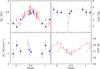 |
Fig. A.2 Mean longitudinal magnetic field (top left), crossover (bottom left), mean quadratic magnetic field (top right), and mean magnetic field modulus (bottom right) of the star HD 2453, against rotation phase. For the longitudinal field, measurements of Babcock (1958; open triangles) and Wolff (1975; crosses) are also shown. The other symbols are as described at the beginning of Appendix A. |
In this Appendix, we discuss the measurements that we obtained for each star individually and their implications for our knowledge of its properties. This discussion is illustrated by figures showing the curves of variation of the mean magnetic field modulus, and when available, the mean longitudinal magnetic field, the crossover, and the quadratic field. Those variations are plotted against the rotation phase, when the period is known, or against the time of observation. In the former case, the fits of the variation curves computed with the parameters listed in Tables 8 to 11 are also shown. The different symbols used to represent the ⟨ B ⟩ data of Paper I and of this paper distinguish the various instrumental configurations with which those measurements have been obtained, as specified in Table 3. In the plots of ⟨ Bz ⟩, ⟨ Xz ⟩ , and ⟨ Bq ⟩, filled dots (navy blue) correspond to the new determinations reported in this paper. For our older data, we used the same symbols as Mathys & Hubrig (1997), namely open squares (brown) for the measurements that these authors obtained with the long camera of CASPEC, filled triangles (violet) for those that they dervived from CASPEC short camera spectra, and filled squares (salmon) for the earlier data of Mathys (1994, 1995a,b). In a few cases, values of some of the magnetic field moments that were obtained by other authors are also included in the figures; the symbols used for that purpose are specified in the individual captions of the relevant figures. Solid curves (red) represent fits for which all parameters are formally significant, long-dashed curves (navy blue) represent fits including a first harmonic that is not formally significant, and short-dashed curves (green) represent non-significant fits by the fundamental only.
For a number of stars for which the diagnostic lines used for the new determinations of ⟨ Bz ⟩, ⟨ Xz ⟩ , and ⟨ Bq ⟩ of this paper show significant intensity variations, figures showing the equivalent widths of those lines against rotation phase are included.
The orbital solutions that we derived for several spectroscopic binaries and the radial velocity measurements for other stars whose radial velocity is variable are also illustrated. The symbols of Table 3 were used to represent the determinations based on the high-resolution spectra recorded in natural light that were analysed in Paper I and in this paper. The individual figure captions specify the symbols used for all other radial velocity measurements, whether based on the CASPEC spectropolarimetric observations of Mathys (1991), Mathys & Hubrig (1997), and this paper, or published by other authors.
Appendix A.1: HD 965
While it had hardly been studied prior to the discovery of resolved magnetically split lines in its spectrum (Paper I), HD 965 has since turned out to be a very unusual and intriguing object. Interest in this star originally arose from our realisation, as part of the present analysis of its CASPEC spectra, of the many apparent similarities between its spectrum and that of HD 101065 (Przybylski’s star), the most peculiar Ap star known. The resemblance was fully confirmed from consideration of higher resolution spectra by Hubrig et al. (2002), who further characterised HD 965 with preliminary quantitative abundance determinations. Like for HD 101065, the hydrogen Balmer lines of HD 965 show a marked core-wing anomaly; both stars were among the first in which this anomaly was identified (Cowley et al. 2001). It reflects the fact that the atmospheric structure of the star is not normal. More remarkably still, the strongest evidence yet for the presence of promethium (an element with no stable isotope) in the spectrum of an Ap star was found in HD 965 (Cowley et al. 2004). However, rather intriguingly, despite its many features in common with Przybylski’s star and other roAp stars, all attempts to detect pulsation in HD 965 so far have yielded negative results (Elkin et al. 2005a).
The richness of the spectrum of HD 965 makes it difficult to find lines sufficiently free from blends to be usable for determination of the longitudinal field, the crossover, and the quadratic field. As a result, the line set from which these field moments were derived is, together with that of HD 47103, the smallest of all the stars analysed here. All diagnostic lines used are Fe i lines, except for one Fe ii line. No significant variation of the equivalent width of these lines was detected, so that there is no indication of large inhomogeneities in the distribution of the element on the stellar surface.
The magnetic measurements of HD 965 are plotted against time in Fig. A.1. After its monotonic decrease observed over the whole time span of the data published in Paper I, the mean field modulus apparently went through a minimum between August 1996 and June 1998 (unfortunately no high-resolution spectrum of the star was obtained between these two epochs). The position in the plot of the last three measurements with respect to the previous points suggests that the slope of the post-minimum increase of ⟨ B ⟩ is significantly less steep than that of its pre-minimum decrease. This is fully confirmed by the more recent data shown in Fig. 3 of Elkin et al. (2005a), which indicates a broad, almost flat minimum over approximately seven years with possibly a shallow secondary maximum around the middle of this time interval. With this feature, the field modulus variation curve is reminiscent of those of other stars discussed here, such as HD 187474 (Fig. A.62). But the duration of the minimum in HD 965 is exceptionally long.
Elkin et al. (2005a) and Romanyuk et al. (2014) also reported new mean longitudinal magnetic field measurements obtained after those presented here. Although systematic differences between ⟨ Bz ⟩ determinations performed with different instruments are not unusual, the combination of the two data sets unambiguously indicates that the longitudinal field of HD 965 went through a negative extremum sometime during the broad minimum of its field modulus (possibly close to the shallow secondary maximum). The difference of slope in the variation of ⟨ Bz ⟩ before and after the time of negative extremum suggests that the field is not symmetric about an axis passing through the centre of the star. The new ⟨ Bz ⟩ data of Elkin et al. (2005a) and Romanyuk et al. (2014) also reveal that the field reverses its polarity along the stellar rotation cycle. This cycle has not yet been fully covered by all the observations obtained until now; the rotation period must significantly exceed 13 yr.
The quadratic field does not show any definite variation over the time span covered by our observations. The ratio between it and the field modulus is remarkably high, reaching of the order of 1.8. This suggests that the field must be unusually inhomogeneous over the observed part of the star.
With the very long rotation period, no significant crossover was expected. Consistently with this, none of the individual determinations of this quantity yield values significantly different from zero (in the best case, a 2.8σ value is obtained). But the facts that all measurements are negative, and that they seem to show a monotonic trend with time towards increasingly negative values, could be regarded as rather convincing indications that crossover is actually detected. This is further discussed in Sect. 5.3.
Appendix A.2: HD 2453
For determination of all magnetic field moments but the mean field modulus in HD 2453, a set of lines of Fe ii was analysed. No variability of the equivalent widths of these lines was observed.
Our five new determinations of the mean longitudinal magnetic field were combined with previous measurements of Babcock (1958), Wolff (1975), and Mathys & Hubrig (1997) to redetermine the rotation period of the star. Some uncertainty arises from the possibility that our determinations may yield values that are systematically 100–200 G more negative than those of Babcock and Wolff. Taking that uncertainty into account, we confirm the best value of the period already adopted in Paper I: Prot = (521 ± 2) d. Using this period, we derive a revised phase origin coinciding with the minimum of ⟨ Bz ⟩, HJD0 = 2 442 288.0. These values of Prot and HJD0 are used to compute the phases against which the various magnetic field moments are plotted in Fig. A.2.
The inclusion of four new measurements of ⟨ B ⟩ into the plot of this field moment against phase increases the scatter about a smooth curve with respect to Fig. 6 of Paper I, to the extent that one may be inclined to question the reality of the detection of actual variations. This doubt is also fuelled by the comparatively low value (0.77) of the multiple correlation coefficient R corresponding to the fit of the ⟨ B ⟩ data with a cosine wave. It should be noted, however, that a large part of the impression of scatter is due to the point corresponding to the single observation of this star with the CFHT. It has been seen in Paper I, and is shown again elsewhere in the present paper, that for a number of stars, differences exist between ⟨ B ⟩ values based on AURELIE observations and on observations obtained with other instruments; these differences are systematic for a given star but vary from star to star for reasons that are not fully understood. Although such differences have not been identified previously for CFHT/Gecko data (of which, between Paper I and this work, we have considerably less than AURELIE data), it is not implausible that they may exist for some stars: HD 2453 may be one of these stars. This view is supported by the fact that, if the CFHT point is removed from the data set, the multiple correlation coefficient is significantly increased for a fit of the remaining data by a cosine wave: R = 0.90. The fit coefficients appearing in Table 8 and the fitted curve shown in Fig. A.2 correspond to this case. The excellent coincidence of the phase of maximum of the mean magnetic field modulus and of the phase of minimum (i.e. largest negative value) of the mean longitudinal magnetic field represents a further indication that we very probably do detect the actual variations of ⟨ B ⟩.
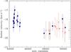 |
Fig. A.3 Our radial velocity measurements for HD 2453 are plotted together with those of Carrier et al. (2002) against heliocentric Julian date. Dots correspond to the Carrier et al. data; all other symbols refer to our high-resolution spectra obtained with various instrumental configurations, as indicated in Table 3. |
By contrast, no definite variation is observed for the quadratic field. The five measurements of this paper, which are much more precise than the determination of Mathys & Hubrig (1997), line up nicely along a cosine curve. But this may be coincidental as the fitted amplitude is only at the 2.5σ level.
None of the individual values derived for the crossover have significance levels above 2.6σ, so that no definite detection is achieved from any of them separately. It is, however, surprising that all of them are negative. This is further discussed in Sect. 5.3.
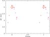 |
Fig. A.4 Mean magnetic field modulus of the star HD 9996, against rotation phase. The symbols are as described at the beginning of Appendix A. |
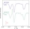 |
Fig. A.5 Portion of the spectrum of HD 9996 recorded at two different epochs (resp. rotation phases), identified above (resp. below) each tracing (the epochs are given as HJD−2 400 000), showing the lines Cr ii λ 6147.1, Fe ii λ 6147.7, and Fe ii λ 6149.2. At the second epoch, the blue wing of the latter is blended with an unidentified rare earth line. That spectrum is affected by a cosmic ray hit between the lines Cr ii λ 6147.1 and Fe ii λ 6147.7. |
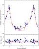 |
Fig. A.6 Upper panel: our radial velocity measurements for HD 9996 are plotted together with those of Carrier et al. (2002) against orbital phase. The solid curve corresponds to the orbital solution given in Table 12. The time T0 of periastron passage is adopted as phase origin. Bottom panel: plot of the differences O−C between the observed values of the radial velocity and the predicted values computed from the orbital solution. The dotted lines correspond to ± 1 rms deviation of the observational data about the orbital solution (dashed line). Dots represent the data from Carrier et al.; all other symbols refer to our high-resolution spectra obtained with various instrumental configurations, as indicated in Table 3. |
Carrier et al. (2002) noted the occurrence of significant radial velocity variations in HD 2453. As can be seen in Fig. A.3, their measurements cluster in two separate time intervals: 14 from HJD 2 444 464 to HJD 2 445 228, whose mean is (−18.00 ± 0.56) km s-1, and 5 from HJD 2 447 958 to HJD 2 450 349, corresponding to a mean value of (−18.92 ± 0.59) km s-1. In each interval, the standard deviation of the measurements is consistent with their errors. Our measurements are mostly contemporaneous with those of the second group of Carrier et al. Combining the latter with those derived from our 13 high-resolution observations of the star (obtained between HJD 2 448 166 and HJD 2 450 797), the resulting mean radial velocity is (− 19.04 ± 0.40) km s-1, which is fully consistent with the value computed from data from Carrier et al. alone. In other words, we confirm that no variations are detected during each of the two considered time intervals. But the ~1 km s-1 difference in the mean value of the radial velocity between them, though small, is significant. Thus HD 2453 appears to be a spectroscopic binary. Even in combination with those of Carrier et al. (2002), our data are insufficient to characterise its orbit. But the orbital period must be (much) longer than the time interval HJD 2 447 958–2 450 797, ~2850 d (or close to 8 yr). The poorer accuracy of the radial velocity determinations achieved from the spectropolarimetric CASPEC observations makes them unsuitable for consideration in this discussion, given the low amplitude of the radial velocity variations observed in HD 2453. We have also omitted them from Fig. A.3.
Appendix A.3: HD 9996
HD 9996 is located too far north to be observable from La Silla. Accordingly, we have not obtained any spectropolarimetric observations for this star. But the variations of its mean longitudinal magnetic field have been monitored over a long time span by the Bychkov group at the Special Astrophysical Observatory (Bychkov et al. 1997, 2012; Metlova et al. 2014).
The three new measurements of the mean magnetic field modulus that are presented here fully confirm that ⟨ B ⟩ went through its maximum at the end of 1993 or the beginning of 1994, as suspected in Paper I. This coincides roughly with the negative extremum of the longitudinal field, which is taken as the phase origin in the ephemeris of Metlova et al. (2014) used to plot the variation of the field modulus in Fig. A.4. In an additional spectrum taken with AURELIE in December 1997 (HJD 2 450 797.312), the line Fe ii λ 6149 is no longer resolved, as shown in Fig. A.5. The interval of approximately seven years separating the two spectra appearing in this figure, which correspond to our first (Mathys & Lanz 1992) and last observations of the star, represents about one-third of its rotation period (Metlova et al. 2014). The field modulus in December 1997 must have been significantly lower than 3.5 kG. Because of the unusually large width of the resolved line components in HD 9996, pointed out in Paper I, the limit of resolution of the Fe ii λ 6149 line in this star is considerably higher than the 1.7 kG limit estimated in Paper I for the majority of slowly rotating Ap stars.
The weak line appearing as a blend in the blue wing of Fe ii λ 6149 in the more recent spectrum is seen, with different intensities, in many Ap stars. It is not definitely identified but undoubtedly pertains to a rare earth element (REE). The fact that it was not seen in our previous spectra but starts to become visible at the end of our sequence of observations is consistent with the fact that the part of the stellar disk where REEs are concentrated is progressively coming into view as a result of stellar rotation, in the transition from REE minimum and magnetic maximum to REE maximum (Rice 1988) and magnetic minimum.
The similarity of the line shapes in the two spectra shown in Fig. A.5 (note in particular the unusual triangular shape of Cr ii λ 6147.1, already noted in Paper I), which were obtained before and after the mean field modulus maximum (see Fig. A.4), suggests that the structure of the magnetic field on the surface of the star, while unusually inhomogeneous, is to some extent symmetrical about the plane defined by the rotation and magnetic axes. On the other hand, a fit of the existing ⟨ B ⟩ measurements by a function of the form of Eq. (16) (that is, by a single sinusoid) leads to a negative minimum of the mean field modulus (of the order of −1.1 kG), which is of course non-physical. This clearly indicates that the actual curve of variation of this field moment must have a high degree of anharmonicity, presumably with a broad, almost flat minimum, similar to other very long period stars (e.g. HD 965, as discussed in Sect. A.1).
HD 9996 is a spectroscopic binary (Preston & Wolff 1970) whose orbital period, Porb = 273 d, is much shorter than the rotation period of the Ap primary. Combining our radial velocity measurements with those of Carrier et al. (2002), we computed a revised orbital solution. Its parameters, which are reported in Table 12, do not significantly differ from those derived by Carrier et al., but their standard deviations are somewhat smaller. The fitted orbit is shown in Fig. A.6.
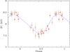 |
Fig. A.7 Mean magnetic field modulus of the star HD 12288, against rotation phase. |
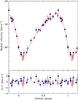 |
Fig. A.8 Upper panel: our radial velocity measurements for HD 12288 are plotted together with those of Carrier et al. (2002) against orbital phase. The solid curve corresponds to the orbital solution given in Table 12. The time T0 of periastron passage is adopted as phase origin. Bottom panel: plot of the differences O−C between the observed values of the radial velocity and the predicted values computed from the orbital solution. The dotted lines correspond to ±1 rms deviation of the observational data about the orbital solution (dashed line). Dots represent the data from Carrier et al.; all other symbols refer to our high-resolution spectra obtained with various instrumental configurations, as indicated in Table 3. |
Appendix A.4: HD 12288
The eight new ⟨ B ⟩ measurements presented in this paper, combined with the data of Paper I, were used by Wade et al. (2000c) to obtain a refined value of the rotation period of HD 12288: Prot = (34.9 ± 0.2) d. The corresponding phase diagram is shown in Fig. A.7; the variation of the field modulus seems to have a slightly anharmonic character, although it is not formally significant (see Table 8). Its maximum coincides roughly, but possibly not exactly, with the minimum of the longitudinal field (i.e. its largest absolute value), according to the measurements of Wade et al. (2000c) of the latter. We could not obtain additional data on that field moment, nor on the crossover or the quadratic field, owing to the northern declination of the star.
The variability of the radial velocity of HD 12288 was announced in Paper I. Since then, Carrier et al. (2002) determined the orbital elements of this binary from a separate set of data, contamporaneous with ours. Here we combined both sets to obtain the revised orbital solution presented in Table 12 and illustrated in Fig. A.8. It is fully consistent with that of Carrier et al., but significantly more precise.
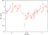 |
Fig. A.9 Mean magnetic field modulus of the star HD 14437, against rotation phase. The symbols are as described at the beginning of Appendix A. |
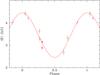 |
Fig. A.10 Mean magnetic field modulus of the star HD 18078, against rotation phase. The symbols are as described at the beginning of Appendix A. |
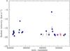 |
Fig. A.11 Our radial velocity measurements for HD 18078 are plotted together with those of Carrier et al. (2002) against heliocentric Julian date. Dots correspond to the Carrier et al. data; all other symbols refer to our high-resolution spectra obtained with various instrumental configurations, as indicated in Table 3. |
Appendix A.5: HD 14437
Like for HD 12288, we could not obtain spectropolarimetric observations of HD 14437 owing to its northern declination. Wade et al. (2000c) published a set of mean longitudinal magnetic field measurements of this star, from which they established the value of its rotation period,  . They also obtained a similar, but less accurate value from analysis of the field modulus data of Paper I, complemented by the 15 new measurements presented here. The variation of ⟨ B ⟩ with this period shows no significant anharmonicity (see Fig. A.9).
The longitudinal field is negative throughout the rotation period. The near coincidence of the phase at which it reaches its most negative value with the phase of the minimum of the field modulus is not the expected behaviour for a centred dipole, from which the actual structure of the magnetic field must significantly depart.
Appendix A.6: HD 18078
The rotation period of HD 18078, Prot = 1358 d, was recently derived (Mathys et al. 2016) by combining our magnetic field modulus measurements (including five new determinations that did not appear in Paper I) with longitudinal field data obtained at the Special Astrophysical Observatory. This makes it one of only five Ap stars for which a period longer than 1000 d has been exactly determined.
Like in HD 9996, the Fe ii λ 6149 line in HD 18078 is magnetically resolved only over part of the rotation cycle, and the resolution limit, close to 2.6 kG, is considerably higher than we would expect in the best cases (~1.7 kG), owing to the fact that the split components are exceptionally broad. This indicates that the geometrical structure of the magnetic field must significantly depart from a simple dipole, which is a conclusion that is further strengthened by the consideration of the variations of the field moments (see Tables 8 and 9). The combination of an anharmonic ⟨ Bz ⟩ curve with a ⟨ B ⟩ curve that does not significantly depart from a sinusoid (Fig. A.10) is highly unusual, as is the large phase shift between their respective extrema. The very high value of the ratio between the maxium and minimum of the mean field modulus, ~1.8, is another manifestation of considerable departures from a dipolar structure.
Carrier et al. (2002) infer that HD 18078 may be a spectroscopic binary with an orbital period of the order of 978 d and a very excentric orbit, from the fact that two of their radial velocity measurements yield values much higher than all others. Our data, which are contemporaneous with theirs, lends some support to this suggestion. In particular, in Fig. A.11 we note how our point obtained on HJD 2 449 286 is higher than the others, which is consistent with the Carrier et al. measurements around the same epoch indicating the probable presence of a narrow peak in the radial velocity curve.
Appendix A.7: HD 29578
The nine new measurements of the mean magnetic field modulus of HD 29578 presented in this paper show a monotonic increase of this field moment and indicate that all the data points of Paper I were concentrated around its phase of minimum (see Fig. A.12). This phase likely coincides approximately with the negative extremum of the mean longitudinal magnetic field. Our nine determinations of this field moment also show a monotonic increase, and it is almost certain that a change of polarity occurred some time after our last spectropolarimetric observation. This extrapolation is borne out by consideration of the variation curve of the mean field modulus, assuming that, as is most frequent (see Fig. 11), its extrema roughly coincide with those of the longitudinal field curve. Indeed, later measurements of ⟨ B ⟩ by Ryabchikova et al. (2004b) show that the monotonic increase of this quantity continued for more than two years after our last determination, leading these authors to suggest that the rotation period should exceed 12 yr. We do not necessarily concur with that conclusion, which is based on the implicit assumption that the ascending and descending slopes in the variation curve of the field modulus are similar. Several counterexamples in the present work show that this cannot be taken for granted. But in any case the period of HD 29578 must be significantly longer than the seven year time span between our first observation and the most recent point of Ryabchikova et al. As also pointed out by Ryabchikova et al., the ratio between the highest value of ⟨ B ⟩ obtained so far and the minimum of this field moment, of the order of 2.0 or greater, is exceptionally large.
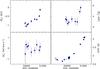 |
Fig. A.12 Mean longitudinal magnetic field (top left), crossover (bottom left), mean quadratic magnetic field (top right), and mean magnetic field modulus (bottom right) of the star HD 29578, against heliocentric Julian date. The symbols are as described at the beginning of Appendix A. |
The quadratic field, after remaining approximately constant since our first point, seems to show a sudden increase in our last two measurements. We would discard this very unusual and surprising behaviour as spurious, if a somewhat similar feature did not also seem to be present for the longitudinal field. Indeed, the determinations of the longitudinal field and the quadratic field are fundamentally different (wavelength shift between lines recorded in opposite circular polarisations against line broadening in natural light), so that it is not very plausible that both are affected by the same errors. If the effect is real, it suggests that the magnetic field of HD 29578 must have a very peculiar structure. Yet the ratio of the quadratic field to the field modulus is similar to that of most stars considered here.
No crossover is detected, which is consistent with the expectation for a star with such a long rotation period. The diagnosis of ⟨ Bz ⟩, ⟨ Xz ⟩, and ⟨ Bq ⟩ is based on the analysis of lines of Fe i, which show no significant variation of equivalent width with time. No radial velocity variation is detected either.
As announced in Paper I, HD 29578 is a spectroscopic binary; its orbital elements, which appear in Table 12, are determined here for the first time. The fitted orbit is shown in Fig. A.13. The orbital period, though long (Porb = 927 d), is much shorter than the rotation period of the Ap primary.
Appendix A.8: HD 47103
Paper I did not include any measurement of HD 47103, in which the presence of resolved magnetically split lines had been announced only shortly before publication (Babel et al. 1995). The region of the spectrum around the line Fe ii λ 6149.2 is shown in Fig. A.14. Four of our determinations of the mean magnetic field modulus are based on ESO-CES spectra; the other three come from different instruments; these data are plotted in Fig. A.15. The CES measurements are very similar; their standard deviation is only 70 G, which is very small compared to the magnetic field strength (~17 kG). The other three values of ⟨ B ⟩ are several hundred Gauss greater. This difference seems unlikely to reflect the occurrence of actual variations of the stellar field, as this would imply that all four CES observations were obtained at either of two phases at which the field modulus had the same value (assuming a typical single-wave variation of this field moment). The probability of such a chance coincidence is very low. Thus we are inclined to suspect that the observed differences between our measurements obtained with different instruments are caused by systematic instrumental effects, whose nature cannot be further assessed because of the small number of observations.
The assumption that the field modulus of HD 47103 remained constant over the time interval covered by our observations (nearly three years), is further supported by the fact that, within the limits of the uncertainties related to the use of different instruments and a different diagnostic method, our ⟨ B ⟩ data are also consistent with the seven measurements published by Babel & North (1997). The latter show no variations over a time range of ~1.5 yr, partly overlapping with the time range during which our observations were obtained. By contrast, Ryabchikova et al. (2008) measured ⟨ B ⟩ = 16.3 kG from a single ESO UVES spectrum obtained about three years after our latest observation. This value of the field modulus is significantly smaller than those we determined from our CES spectra, and barring systematic differences between the two instruments, it may be suggestive of a slow decrease of ⟨ B ⟩ over the considered time span, hence of a long period (or the order of years).
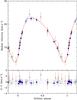 |
Fig. A.13 Upper panel: our radial velocity measurements for HD 29578 are plotted against orbital phase. The solid curve corresponds to the orbital solution given in Table 12. The time T0 of periastron passage is adopted as phase origin. Bottom panel: plot of the differences O−C between the observed values of the radial velocity and the predicted values computed from the orbital solution. The dotted lines correspond to ±1 rms deviation of the observational data about the orbital solution (dashed line). Open squares represent our CASPEC observations; all other symbols refer to our high-resolution spectra obtained with various instrumental configurations, as indicated in Table 3. |
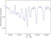 |
Fig. A.14 Portion of the spectrum of HD 47103 recorded on HJD 2 450 427.689, showing the lines Cr ii λ 6147.1 (affected by a cosmic ray hit), Fe ii λ 6147.7, and Fe ii λ 6149.2. |
At present, we adopt 70 G as the estimated uncertainty of our ⟨ B ⟩ measurements of HD 47103, bearing in mind the fact that, like for HD 192678 (Paper I), this value corresponds to random measurement uncertainties, but ignores possible systematic instrumental errors.
HD 47103 has one of the strongest magnetic fields known. As a result, even at moderate spectral resolutions, many of its spectral lines are resolved into their Zeeman components, or at least are strongly broadened. This makes it difficult to find lines sufficiently free from blends for magnetic field diagnosis from the CASPEC spectra. Accordingly the set of lines used for this purpose is smaller than for any other star studied in this paper but HD 965. As a consequence, it was not possible to use the multi-parameter fit described in Sect. 3.2 for determination of the mean quadratic magnetic field. Instead the simpler, less accurate form of the fit function given in Eq. (14) was adopted. This is not expected to have a major impact in the present case, since the magnetic field is by far the dominant broadening factor and the accuracy of its determination should not be strongly affected by approximate treatment of the other contributions to the line width. All the lines used for determination of ⟨ Bz ⟩, ⟨ Xz ⟩, and ⟨ Bq ⟩ are Fe i lines, except for one Fe ii line. They show no significant equivalent width variations.
Variation of the longitudinal field is not definitely detected in our data, although there is some hint in Fig. A.15 that it may have undergone a slow, monotonic variation from less negative to more negative values over the time span covered by our observations. However, this apparent trend is probably only coincidental. It vanishes when combining our data with eight additional ⟨ Bz ⟩ measurements obtained by Elkin & Wade (1997) over a period slightly shorter than two months, which includes the date of our first CASPEC observation of HD 47103. These measurements are more scattered than ours. A period search combining both data sets remained inconclusive.
No definite variation of the quadratic field is seen either. The ratio of ⟨ Bq ⟩ to ⟨ B ⟩ is marginally smaller than one. Formally, this is physically meaningless and may at first sight suggest that the quadratic field has been systematically underestimated in this star. But taking the measurement uncertainties into account, the discrepancy vanishes; considering the high value of the field modulus, compared to the longitudinal field, it is not unexpected that ⟨ Bq ⟩ hardly differs from ⟨ B ⟩. On the other hand, from better observational data, Mathys & Hubrig (2006) obtained from analysis of a set of Fe i lines ⟨ Bq ⟩ = 19.3 ± 0.5 kG on HJD 2 450 115.615 (that is, one week after the first measurement reported here). This value is more consistent with the field modulus, and the difference between it and most measurements of this paper, though somewhat marginal, is formally significant. Thus we cannot fully rule out the possibility that the ⟨ Bq ⟩ values reported here for this star are systematically underestimated, plausibly because of the above-mentioned application of the simplified Eq. (14) to derive them.
No crossover is detected, but the error bars are among the largest for any star in this paper.
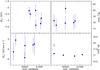 |
Fig. A.15 Mean longitudinal magnetic field (top left), crossover (bottom left), mean quadratic magnetic field (top right), and mean magnetic field modulus (bottom right) of the star HD 47103, against heliocentric Julian date. The symbols are as described at the beginning of Appendix A. |
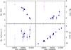 |
Fig. A.16 Mean longitudinal magnetic field (top left), crossover (bottom left), mean quadratic magnetic field (top right), and mean magnetic field modulus (bottom right) of the star HD 50169, against heliocentric Julian date. The symbols are as described at the beginning of Appendix A. |
The lack of definite variations of any of the observables that we considered implies that either HD 47103 has an extremely long period, or that for this star, one at least of the angles i (between the rotation axis and the line of sight) or β (between the magnetic and rotation axes) is too close to zero for any detectable variability to occur. Longer term follow-up of the star is needed to solve this ambiguity. This is an especially important issue, as a very long period, if confirmed, would make HD 47103 an exception to the conclusion that fields stronger than 7.5 kG occur only in stars with rotation periods shorter than 150 d (see Sect. 5.1).
Babel & North (1997) and Carrier et al. (2002) report a possible variability of the radial velocity in HD 47103. The scatter of our radial velocity measurements supports this possibility, but the data currently available are insufficient to set significant constraints on the orbital period.
Appendix A.9: HD 50169
The monotonic increase of the mean magnetic field modulus of HD 50169 noted in Paper I continues throughout the time span covered by the new observations presented here, indicating that the rotation period of the star must be much longer than the 7.5 yr separating our oldest determination of this quantity from the most recent one (see Fig. A.16).
Our measurements of the other field moments, combined with the single one of Mathys & Hubrig (1997), are spread over five years. During this interval the longitudinal field showed a monotonic decrease. There is some hint in both the ⟨ B ⟩ and ⟨ Bz ⟩ curves that an extremum may have taken place not too long before our first observations, suggesting that phases of minimum of the field modulus and of positive extremum of the longitudinal field may roughly coincide. The monotonic increase of ⟨ Bz ⟩ observed by Babcock (1958) over a three-year time span is approximately mirror symmetric with the decrease that we recorded over a similar time range in our observations (Fig. A.17), but the more than 40 yr of separation between the epochs of the Babkock observations and ours does not allow us to be sure that both pertain to the same rotation cycle. Actually it seems somewhat more likely that at least one full rotation cycle has been completed in between. This is consistent with the more recent measurement of Romanyuk et al. (2014), also shown in Fig. A.17, which is the only one until now to yield a negative value of ⟨ Bz ⟩ and establishes that both poles of the star come into view in alternation.
Over the three years covered by the new spectropolarimetric CASPEC data analysed here, the quadratic field shows a slow, but definite monotonic increase, roughly following that of the field modulus. The single measurement of Mathys & Hubrig (1997) has a large formal uncertainty, and its deviation from the general trend more probably reflects its low quality rather than the actual behaviour of the star. No significant crossover is detected.
The determinations of ⟨ Bz ⟩, ⟨ Xz ⟩ , and ⟨ Bq ⟩ are based on the analysis of a set of lines of Fe ii, which show no equivalent width variations.
The variability of the radial velocity of HD 50169 was reported for the first time in Paper I. Combining our radial velocity measurements with those of Carrier et al. (2002), we achieved the first determination of its orbital parameters, which are presented in Table 12. The fitted orbit is shown in Fig. A.18. That the orbit could be determined despite the low amplitude of the radial velocity variations of this star (less than 4 km s-1 peak-to-peak) and its long orbital period (almost five years long – still much shorter than the rotation period of the Ap primary) is testament to the precision and the stability of our radial velocity determinations.
Appendix A.10: HD 51684
The presence of resolved magnetically split lines in HD 51684 was discovered as part of this project after Paper I was written, and it is reported here for the first time. We are not aware of any attempt to study the magnetic field of this star prior to this discovery. A portion of a high-resolution spectrum around the line Fe ii λ 6149.2 is shown in Fig. A.19. The sharpness of the split components of this line and the fact that the spectrum goes back almost all the way up to the continuum between them reflect the narrow spread of the magnetic field strengths over the stellar disk.
Only the mean magnetic field modulus measurements lend themselves to determination of the rotation period, for which the value Prot = (371 ± 6) d was obtained. Our data are plotted against this period in Fig. A.20. Their standard deviation about the best-fit curve of the form given in Eq. (16) is 25 G. We adopted this value for the uncertainties of our ⟨ B ⟩ measurements of this star.
Because the rotation period of HD 51684 is unfortunately close to one year, the distribution across the rotation cycle of our spectropolarimetric observations, which are less numerous than our high-resolution spectra in natural light, is very uneven. Nevertheless, the longitudinal field data unambiguously rule out a much shorter period, of the order of 105, which looks plausible from consideration of the ⟨ B ⟩ data alone. While both ⟨ B ⟩ and ⟨ Bz ⟩ undergo definite variations, the shape of their variation curves is not strongly constrained (especially in the case of ⟨ Bz ⟩) by the available data. But the existence of a considerable phase shift between their respective extrema seems inescapable since the variation of ⟨ Bz ⟩ is very steep around the phase of minimum of ⟨ B ⟩.
Out-of-phase variations of the longitudinal field and the field modulus represent an unusual feature among the stars studied here, which is suggestive of a magnetic field structure significantly different from a simple dipole. This is rather surprising, since sizeable departures from a centred dipole tend to spread the distribution of the field strengths across the stellar surface, which manifests itself observationally by a broadening of the resolved line components, such as observed in for example HD 9996 (see Fig. A.5) or HD 18078 (see Fig. 1 of Mathys et al. 2016). As explained above, this effect is definitely not apparent in HD 51684. Further investigation is warranted to identify a magnetic field structure that can account for both the phase shift between the variations of ⟨ B ⟩ and ⟨ Bz ⟩ and the very clean profiles of the resolved split lines.
On the other hand, it appears unlikely that ⟨ Bz ⟩ reverses its sign over the rotation cycle. If the field of HD 51684 bears any resemblance to a dipole, it is probable that only its negative pole is observed. The quadratic field shows no definite variation over the covered phase range, and no significant detection of the crossover is achieved, which is consistent with the length of the rotation period.
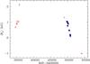 |
Fig. A.17 Mean longitudinal magnetic field of the star HD 50169, against heliocentric Julian date. Crosses represent the measurements of Babcock (1958), and the filled square is the point obtained by Romanyuk et al. (2014). The other symbols are as described at the beginning of Appendix A. |
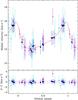 |
Fig. A.18 Upper panel: our radial velocity measurements for HD 50169 are plotted against orbital phase. The solid curve corresponds to the orbital solution given in Table 12. The time T0 of periastron passage is adopted as phase origin. Bottom panel: plot of the differences O−C between the observed values of the radial velocity and the predicted values computed from the orbital solution. The dotted lines correspond to ± 1 rms deviation of the observational data about the orbital solution (dashed line). Open triangles represent the data from Carrier et al. and asterisks our CASPEC observations; all other symbols refer to our high-resolution spectra obtained with various instrumental configurations, as indicated in Table 3. |
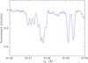 |
Fig. A.19 Portion of the spectrum of HD 51684 recorded on HJD 2 450 427.623, showing the lines Cr ii λ 6147.1, Fe ii λ 6147.7, and Fe ii λ 6149.2. |
The determination of ⟨ Bz ⟩, ⟨ Xz ⟩ , and ⟨ Bq ⟩ is based on the analysis of a mixed set of Fe i and Fe ii lines. These lines are found to undergo equivalent width variations with an amplitude of the order of 10%; the lines appear weaker close to phase 0.5, that is, close to the phase of minimum of the field modulus. The exact phases of extrema are somewhat uncertain, however, owing to the poor sampling of the rotation cycle by our observations. The variability of the equivalent widths means that the distribution of Fe on the surface of HD 51684 is less uniform than in most Ap stars. As the amplitude of the variations is rather small, the inhomogeneities are not extreme, and their impact on the derived values of the field moments should be limited. Nevertheless one should keep in mind in the interpretation of those moments that they represent the convolution of the actual structure of the magnetic field with the distribution of Fe over the stellar surface.
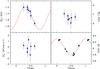 |
Fig. A.20 Mean longitudinal magnetic field (top left), crossover (bottom left), mean quadratic magnetic field (top right), and mean magnetic field modulus (bottom right) of the star HD 51684, against rotation phase. The symbols are as described at the beginning of Appendix A. |
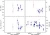 |
Fig. A.21 Mean longitudinal magnetic field (top left), crossover (bottom left), mean quadratic magnetic field (top right), and mean magnetic field modulus (bottom right) of the star HD 55719, against heliocentric Julian date. The symbols are as described at the beginning of Appendix A. |
Appendix A.11: HD 55719
The 14 new determinations of the mean magnetic field modulus of HD 55719 presented here definitely rule out the tentative values of the period proposed in Paper I (847 d or 775 d). Instead, one can see in Fig. A.21 that a very slow decrease of ⟨ B ⟩ is becoming apparent. The unexpectedly large scatter of the data points about this long-term trend had previously misled us into believing that we had observed shorter timescale actual variations, but it now clearly appears that the rotation period of the star must vastly exceed the time span covered by our data, which is ~3800 days. The origin of the scatter of the measurements about this slow variation is unclear. The alternative of a very short period, for example close to 1 day, has been ruled out in Paper I. The star is bright, so that virtually all spectra that we have recorded have signal-to-noise ratios amongst the highest of all spectra analysed in this project. The blend of the blue component of Fe ii λ 6149 by an unidentified REE line, which complicates its measurement in many of the studied stars, increasing its uncertainty, has not been seen over the part of the rotation cycle observed so far in HD 55719. The peculiar shape of the split components of Fe ii λ 6149, attributed in Paper I to an unusual structure of the magnetic field, does not introduce particular complications in the measurement of their wavelengths, since they are very well separated (see Fig. 2 of Paper I). As already discussed at length in previous papers (Mathys 1990; Mathys & Lanz 1992), while the star is a double-lined spectroscopic binary (SB2), no feature of the secondary is readily seen in the region around 6150 Å. Admittedly, some contamination of the ⟨ B ⟩ measurements by contribution of the secondary that escapes visual inspection might be present. Considering the very slow variation of the primary, however, we would then expect the orbital period to come out in a frequency analysis of the ⟨ B ⟩ data, but it definitely does not. Furthermore, the quality of the radial velocity data derived from the same measurements of the Fe ii λ 6149 line performed for determination of the field modulus (see below) does not suggest that they are in the least polluted by the secondary spectrum. In summary, for now we do not know what causes the large scatter of the ⟨ B ⟩ data about their long-term trend. Further investigation is needed to identify this cause. But whatever it is, we are confident that it does not question the conclusion that the rotation period of the star must be longer than a decade.
Like the mean magnetic field modulus, the longitudinal field and crossover (mostly null) data show somewhat more scatter than would be expected from their estimated uncertainty. However, for these latter two field moments, a plausible explanation exists. Namely, the set of diagnostic lines (of Fe ii) used for their determination contains a fraction of lines from regions of the spectrum affected by telluric water vapour absorption lines that is considerably higher than for most other stars of the analysed sample. Although the generally very dry conditions on La Silla make these telluric lines much less disruptive than in most other observatory sites, they are variable with the time and with the airmass of the observations, and they can have some effect on the measurements, especially on the most humid nights. These effects, from the point of view of the stellar properties, come in as essentially random noise. This interpretation is all the more plausible since we observed HD 55719 through clouds more often than most other stars because of its brightness. However, it is not entirely supported by consideration of the mean quadratic magnetic field, which appears constant, with little scatter, for the measurements of this paper. The marginal discrepancy of the older two data points of Mathys & Hubrig (1997) can most probably, as in other cases, be attributed to the shortcomings of the quadratic field measurements of this reference. The equivalent widths of the lines used for determination of the field moments from the CASPEC spectra also show some scatter, which is plausibly related to the scatter in the magnetic field data.
We combined our radial velocity measurements to those of Bonsack (1976) to refine the orbital elements originally derived by this author (see Table 12 and Fig. A.22). The orbital period,  , is much shorter than the rotation period of the Ap component.
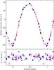 |
Fig. A.22 Upper panel: our radial velocity measurements for HD 55719 are plotted together with those of Bonsack (1976) against orbital phase. The solid curve corresponds to the orbital solution given in Table 12. The time T0 of periastron passage is adopted as phase origin. Bottom panel: plot of the differences O−C between the observed values of the radial velocity and the predicted values computed from the orbital solution. The dotted lines correspond to ±1 rms deviation of the observational data about the orbital solution (dashed line). Open triangles represent the data from Bonsack and open squares our CASPEC observations; all other symbols refer to our high-resolution spectra obtained with various instrumental configurations, as indicated in Table 3. |
Appendix A.12: HD 59435
A complete study of HD 59435, a SB2 with an orbital period  , has been published elsewhere (Wade et al. 1999). It includes the new field modulus measurements obtained since Paper I, which are repeated here for completeness and for comparison with the other studied stars. The rotation period of the Ap component, Prot = 1360 d, is only slightly shorter than the orbital period; Wade et al. argue that this similarity is coincidental. The curve of variation of ⟨ B ⟩ (Fig. A.23) is definitely anharmonic, with a fairly broad, almost flat minimum, that is reminiscent of the behaviour observed in other stars, such as HD 965 (see Appendix A.1) or HD 187474 (see Appendix A.35); the maximum also shows some hint of flattening, albeit less pronounced. It is also worth noting that even though the field modulus was only of the order of 2.3 kG around minimum, the components of the Zeeman doublet Fe ii λ 6149 were clearly resolved and their separation could be measured without major uncertainty. This clearly demonstrates the feasibility of the determination of mean field moduli of that order or even somewhat smaller.
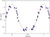 |
Fig. A.23 Mean magnetic field modulus of the star HD 59435, against rotation phase. The symbols are as described at the beginning of Appendix A. |
Based on our previous experience of the intricacies of untangling the contributions of the two components of the binary in our high-resolution spectra recorded in natural light (Wade et al. 1996b), we gave up on attempting to observe the star in spectropolarimetry, so as to save the available telescope time for objects for which we were more confident that it would actually be possible to exploit the data.
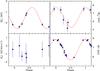 |
Fig. A.24 Mean longitudinal magnetic field (top left), crossover (bottom left), mean quadratic magnetic field (top right), and mean magnetic field modulus (bottom right) of the star HD 61468, against rotation phase. The symbols are as described at the beginning of Appendix A. |
Appendix A.13: HD 61468
The 11 new determinations of the mean magnetic field modulus presented here, combined with the four data points of Paper I, unambiguously define the rotation period of HD 61468: Prot = (322 ± 3) d. This period also matches the variations of the longitudinal field and the quadratic field (see Fig. A.24). The variations of all three field moments are well represented by cosine waves, but the variation curves are only loosely constrained for ⟨ Bz ⟩ and ⟨ Bq ⟩ because of the small number of measurements obtained. Accordingly, the phase shift between the extrema of ⟨ B ⟩ and ⟨ Bq ⟩, on the one hand, and of ⟨ Bz ⟩, on the other hand, cannot be regarded as significant. To the precision achieved, the largest negative value of the longitudinal field coincides with the maxima of the quadratic field and field modulus. The longitudinal field probably does not reverse its polarity as the star rotates, but this cannot be definitely ascertained because of incomplete phase coverage of the observations. The ratio between the extrema of ⟨ B ⟩, close to 1.4, exceeds the limit value for a centred dipole, 1.25, from which its structure must show some departure. The quadratic field also shows an unusually large amplitude of variation. The latter is certainly real, even though, in absolute terms, the fact that ⟨ Bq ⟩ is systematically marginally smaller than ⟨ B ⟩ is non-physical and suggests that it may be somewhat underestimated. However, taking their uncertainties into account, the difference between the two field moments is not significant.
As can be expected from the long rotation period, no significant crossover is detected: no derived value exceeds 2σ. But it is somewhat intriguing that all measurements (but one, which is null) yield negative values.
The equivalent widths of the Fe ii lines, which are used to determine ⟨ Bz ⟩, ⟨ Xz ⟩, and ⟨ Bq ⟩, vary with a full amplitude of the order of 15%. The lines appear to be stronger close to the phase of maximum of the field modulus and weaker around its minimum. This may have a small effect on the measured field moments, which should be kept in mind in their interpretation.
The variability of the radial velocity of the star was pointed out in Paper I. Here we determine an orbital solution for the first time; the parameters of this orbital solution are given in Table 12 and the resulting fit appears in Fig. A.25. At 273, the orbital period of HD 61468, which is considerably shorter than the rotation period of its Ap component, is the shortest one for the known binaries containing an Ap star with resolved magnetically split lines. It is very remarkable that none of these binaries have shorter Porb.
Appendix A.14: HD 65339
HD 65339 is one of the Ap stars whose magnetic field has been best studied. In particular, the Kochukhov et al. (2004) model of its field is one of the most detailed and precise models of an Ap star magnetic field obtained so far. The primary reason why the star is included in the present study is to allow its consideration in the statistical discussion of the properties of the Ap stars with resolved magnetically split lines by characterising it with data of the same nature as for the other members of the class.
The 14 new measurements of the mean magnetic field modulus reported here are plotted together with the data of Paper I in Fig. A.26; the phases are based on the very accurate value of the rotation period of Hill et al. (1998). To the eye, the variations are strongly anharmonic, which is not surprising considering the complexity of the field structure revealed by the Kochukhov et al. (2004) analysis. The variation curve shown in the figure is the best fit by the superposition of a cosine wave and of its first harmonic, but the harmonic term is not formally significant (see Table 8). With the complex structure of the field, such a superposition is not likely to provide a good fit to the data. But we did not try to improve on it, for example by adding higher harmonics, because the points on the descending branch of the variation curve are scarce and the ⟨ B ⟩ determinations involve unusually large uncertainties, owing to the distortion, strong blending, and marginal resolution of the Fe ii λ 6149 line over part of the rotation cycle (see Paper I). Actually considering the difficulty of the measurements, the fairly small dispersion of the data points about a smooth variation curve is rather surprising.
The northern declination of the star did not allow us to obtain spectropolarimetric observations, but there are many published longitudinal field measurements of HD 65339; see Kudryavtsev & Romanyuk (2012) and references therein.
Carrier et al. (2002) determined the orbital parameters of HD 65339 by fitting radial velocity data, speckle measurements, and the Hipparcos parallax of the star simultaneously. Our radial velocity measurements do not add anything to their solution.
Appendix A.15: HD 70331
The seven new measurements of the mean magnetic field modulus of HD 70331 definitely rule out the tentative value of the rotation period  suggested in Paper I. Period determination is hampered by strong aliasing, even with the larger set of ⟨ B ⟩ data of the present study. The most probable values now are Prot = (1.9989 ± 0.0008) d or Prot = (1.9909 ± 0.0008) d. The proximity of these values to two days may raise some concern about their reality. However visual inspection of the spectra reveals the occurrence of considerable variations from one night to the next, and significant distortion of the resolved components of Fe ii λ 6149 by the combination of different amounts of Doppler and Zeeman effects on different parts of the stellar surface. All the field moments are plotted against phases computed with these two periods in Figs. A.27 and A.28. In the former, there may be some very marginal hint of variation of ⟨ Bz ⟩ with the 19989 period. However, the scatter of the individual measurements of this field moment is consistent with its being constant, so that the absence of correlation with phase seen in the other figure for
  does not represent an argument against the reality of that period. A formally significant non-zero rms value of the crossover is computed by combining all individual measurements, but none of these measurements represent definite detections in themselves (in the best case, a 2.6σ value is obtained). Neither the quadratic field nor the equivalent widths of the Fe ii lines used to diagnose the magnetic field from the CASPEC spectra show any definite variability.
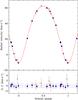 |
Fig. A.25 Upper panel: our radial velocity measurements for HD 61468 are plotted against orbital phase. The solid curve corresponds to the orbital solution given in Table 12. The time T0 of periastron passage is adopted as phase origin. Bottom panel: plot of the differences O−C between the observed values of the radial velocity and the predicted values computed from the orbital solution. The dotted lines correspond to ± 1 rms deviation of the observational data about the orbital solution (dashed line). Open squares represent our CASPEC observations; all other symbols refer to our high-resolution spectra obtained with various instrumental configurations, as indicated in Table 3. |
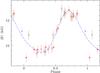 |
Fig. A.26 Mean magnetic field modulus of the star HD 65339, against rotation phase. The symbols are as described at the beginning of Appendix A. |
In any event, there is no question that the rotation period of HD 70331 must be of the order of days. While our data do not lend themselves well to the determination of its v sini, the presence of well-resolved lines in its spectrum – much better resolved than in HD 65339, which has a field of comparable strength and v sini = 12.5 km s-1 (Kochukhov et al. 2004) – indicates that it cannot exceed 10 km s-1. For a star of this temperature, the stellar radius cannot be significantly smaller than 2.5 R⊙, so that the angle between the rotation axis and the line of sight must be at most 10°. With such a low inclination, the amplitude of variation of ⟨ B ⟩ is remarkably large. This suggests the existence of a strongly magnetic spot close to the stellar limb, which alternately comes in and out of view as the star rotates. This is consistent with the absence of large variation of the longitudinal field provided that the magnetic vector in this spot is mostly transversal. The likelihood of such a configuration, in combination with the large magnetic field strength, makes HD 70331 a promising candidate for observations of linear polarisation in spectral lines.
Appendix A.16: HD 75445
The clean, sharp profile of Fe ii λ 6149 in HD 75445 lends itself well to the precise determination of the mean magnetic field modulus. Accordingly, there is little doubt that the range of the derived values of ⟨ B ⟩ reflects actual variations of this field moment. In a period analysis, one value stands out rather clearly: Prot = (6.291 ± 0.002) d. When phased with this period, the ⟨ B ⟩ data closely follow a smooth, though strongly anharmonic, variation curve (Fig. A.29). Given the low amplitude of the variations, a comparison of our data with field values of other authors may not be meaningful, so that we shall restrict ourselves to note that the three measurements of this star by Ryabchikova et al. (2004b) are not inconsistent with the proposed period (or a very close value). Actually they are more consistent with the rather short period proposed here than with the very long period suggested by these authors.
Only three spectropolarimetric observations of the star could be secured, which are insufficient to characterise the variations of the field moments derived from their analysis (based on a set of Fe i lines). Only one of the three values of ⟨ Bz ⟩ that are derived is formally non-null, albeit marginally so (at the 3.0 σ level), and no crossover is detected. By contrast, the quadratic field comes out clearly, and is about 1.4 times greater than the field modulus.
In any event, more observations are required to establish definitely that the value of the period proposed here is correct.
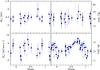 |
Fig. A.27 Mean longitudinal magnetic field (top left), crossover (bottom left), mean quadratic magnetic field (top right), and mean magnetic field modulus (bottom right) of the star HD 70331, against rotation phase, computed assuming that the rotation period is 1 |
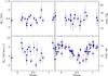 |
Fig. A.28 Mean longitudinal magnetic field (top left), crossover (bottom left), mean quadratic magnetic field (top right), and mean magnetic field modulus (bottom right) of the star HD 70331, against rotation phase, computed assuming that the rotation period is 1 |
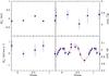 |
Fig. A.29 Mean longitudinal magnetic field (top left), crossover (bottom left), mean quadratic magnetic field (top right), and mean magnetic field modulus (bottom right) of the star HD 75445, against rotation phase. The symbols are as described at the beginning of Appendix A. |
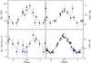 |
Fig. A.30 Mean longitudinal magnetic field (top left), crossover (bottom left), mean quadratic magnetic field (top right), and mean magnetic field modulus (bottom right) of the star HD 81009, against rotation phase. The symbols are as described at the beginning of Appendix A. |
Appendix A.17: HD 81009
The visual and single-lined spectroscopic binary (SB1) HD 81009 was studied in detail by Wade et al. (2000a). This work was based in part on the measurements of the mean magnetic field modulus (only two new determinations since Paper I), mean longitudinal magnetic field and radial velocity that are reported in this paper.
Figure A.30 shows the variations of the four field moments considered here against the rotation phase determined using the refined value of the rotation period derived from photometry by Adelman (1997) and confirmed by Adelman (2006), which is more accurate than the period obtained in Paper I. The variations of all four moments are well represented by cosine waves. The values of the crossover and quadratic field published by Mathys & Hubrig (1997) for their single observation of HD 81009, which are of much poorer quality than the data presented here, have been left out of the fits and do not appear in the figure (where they would be out of scale). The value of the quadratic field, which was obtained by Mathys & Hubrig (2006) from the analysis of a larger set of Fe i lines measured in a higher resolution spectrum covering a broader wavelength range recorded at phase 0.733, ⟨ Bq ⟩ = 9825 ± 438 G, is in excellent agreement with the measurements presented here.
The phases of maximum of the longitudinal field and the quadratic field coincide almost exactly; the maximum of the field modulus seems to occur slightly earlier (about 0.06 rotation cycle), but this phase difference is at the limit of significance. Although none of the individual values of the crossover are formally significant (they are all below 2.7σ), the rms value obtained by combining them indicates a definite detection and they show a formally significant sinusoidal variation with rotation phase, with a fairly high value of the R coefficient, 0.83; this is also apparent visually in Fig. A.30. That we indeed detect the actual variation of the crossover is made all the more plausible by the fact that the curve fitted to the variations of ⟨ Xz ⟩ is, within the errors, in phase quadrature with the ⟨ Bz ⟩ fit; see Sect. 5.3 for a general discussion of the phase relation between these two field moments.
The variability of the Fe i and Fe ii lines from which ⟨ Bz ⟩, ⟨ Xz ⟩ , and ⟨ Bq ⟩ are determined is illustrated in Fig. A.31, where the average  of their normalised equivalent widths (see Mathys 1994, for definition of this quantity) is plotted against rotation phase. The lines are stronger close to the phase of ⟨ B ⟩ maximum. As for other stars, the corresponding differences of local line intensities are convolved into the derived values of the considered field moments.
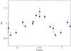 |
Fig. A.31 Variation with rotation phase of the average |
Appendix A.18: HD 93507
Only two new measurements of the mean magnetic field modulus of HD 93507 are reported here, and are plotted in Fig. A.32 together with our previous data against the phase computed using the value of the rotation period derived in Paper I, Prot = 556 d. This period also matches the variations of the other field moments. The longitudinal field is positive throughout the rotation cycle. The phase of its minimum coincides with the phase of ⟨ B ⟩ maximum, indicating that the field structure must significantly depart from a centred dipole. There is a hint of anharmonicity in the variation of ⟨ Bz ⟩, for which the superposition of a cosine wave and of its first harmonic gives a somewhat better fit both visually and mathematically (the reduced χ2 decreases from 1.7 to 1.4 when adding the first harmonic), but is not formally significant. The improvement resulting from inclusion of the first harmonic in the fit is less definite for the quadratic field; we cannot decide at present if the ⟨ Bq ⟩ variation curve actually departs significantly from a single cosine wave, or if its apparent anharmonicity results from some combination of the limited precision of the measurements and of their uneven coverage of the rotation cycle. The fact that ⟨ Bq ⟩ is marginally smaller than ⟨ B ⟩ over a sizable fraction of the stellar rotation cycle indicates that it is probably somewhat underestimated. This discrepancy is more pronounced around phases 0.1–0.2, while the error bars of all field moments are larger in the phase interval 0.4–0.6 than over the rest of the rotation cycle. This appears due primarily to the fact that, around the maximum of the field modulus, the spectral lines show significant distortion, suggesting that the distribution of the magnetic field strength and/or orientation over the corresponding part of the star is much less uniform than on the rest of its surface. The fact that Fe ii lines, from which the field is diagnosed, are weaker around phase 0.5 may also have some impact on the achievable measurement precision, but contrary to what was conjectured in Paper I, it seems unlikely to be the main cause of its degradation. Indeed, the amplitude of variation of the equivalent widths is rather small (see Fig. A.33) – smaller, in particular, than in other stars where these variations have no noticeable effect on the magnetic field determination. The distortion of the spectral lines around phase 0.5 may possibly account for the apparent variation of the crossover around that phase, but they certainly cannot be invoked to explain its consistently positive value over the rest of the period. Actually, it rather looks as though a definite non-zero crossover is detected in this star, which is somewhat unexpected because of its long rotation period. This is further discussed in Sect. 5.3.
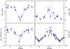 |
Fig. A.32 Mean longitudinal magnetic field (top left), crossover (bottom left), mean quadratic magnetic field (top right), and mean magnetic field modulus (bottom right) of the star HD 93507, against rotation phase. The symbols are as described at the beginning of Appendix A. |
Appendix A.19: HD 94660
The eight new determinations of the mean magnetic field modulus of HD 94660 presented here fully confirm the suspicion expressed in Paper I that the time interval covered by the data of that paper is almost identical to the rotation period of the star. The value of the latter can now be determined from the whole set of ⟨ B ⟩ measurements: Prot = (2800 ± 200) d. This value is in good agreement with that derived independently by Landstreet et al. (2014) from analysis of FORS-1 ⟨ Bz ⟩ data spanning nearly one rotation cycle, Prot = (2800 ± 250) d.
The rather large uncertainty affecting the value of the period reflects the fact that, even with the new observations, the ⟨ B ⟩ data obtained so far cover only ~1.3 rotation cycle. For the same reason, and because of the apparently rather complex shape of the variation of ⟨ B ⟩ around its minimum (see Fig. A.34), the time of the latter, adopted as phase origin, must be regarded as rather uncertain.
The harmonic term of a fit of the field modulus values by a function of the form of Eq. (17) is just below the threshold of formal significance. But the anharmonicity of the curve of variation of ⟨ B ⟩ appears definite. Its asymmetry indicates that the magnetic field of HD 94660 is not symmetric about an axis passing through its centre.
The other field moments are diagnosed from analysis of a set of lines of Fe ii, whose equivalent widths appear constant over the stellar rotation period. Based on the new measurements of the present paper, variations of the quadratic field are undoubtedly observed. But it is far from certain that the fitted curve describes their actual shape, since its determination heavily depends on the older data of Mathys (1995b) and Mathys & Hubrig (1997), derived by application of Eq. (14), which have much larger uncertainties than the new values reported here. We note that, close to phase 0, the values of ⟨ Bq ⟩ are only marginally consistent with those of ⟨ B ⟩, which suggests that they may be somewhat underestimated. However, they are fully consistent with the value obtained by Mathys & Hubrig (2006) from the analysis of a better quality spectrum recorded at phase 0.113.
The new ⟨ Bz ⟩ data of this paper seem to to indicate a slow increase (from more to less negative values) over the time range that they cover. But neither in isolation nor combined with our previous measurements do they undisputedly establish the occurrence of variations of the longitudinal field. The fitted variation curve is not formally significant, and it must therefore be regarded as tentative at best. It is intriguing, though, that within the limits of the uncertainties, this curve is in phase quadrature with the fitted ⟨ Xz ⟩ curve. However, the latter must be taken with even more caution, since it is primarily defined by the difference between the present set of measurements and the old, lower quality data of Mathys (1995a) and Mathys & Hubrig (1997), since none of the crossover determinations (old or new), taken individually, are formally significant (they never exceed 2.6σ), and since crossover is not expected to occur for rotation periods of several years; see Sect. 5.3, however.
That the fitted ⟨ Bz ⟩ curve reflects real variations is furthermore supported by the near coincidence of the phase of the largest negative value of the longitudinal field with that of the minimum of the mean field modulus. While such a phase relation between ⟨ Bz ⟩ and ⟨ B ⟩ indicates that the field structure departs significantly from a centred dipole, it is observed in about half of the stars studied in this paper for which the variation curves of the two field moments are defined (see Sect. 5.2).
On the other hand, we announced in Paper I that the radial velocity of HD 94660 is variable. Preliminary orbital elements were derived by Bailey et al. (2015). They are fully consistent with those obtained from analysis of our data, which sample the orbit more densely. We combined both data sets to determine the refined orbital elements reported in Table 12. The fitted orbit is shown in Fig. A.35. The orbital period, 849 d, is shorter than the rotation period of the Ap component.
Appendix A.20: HD 110066
The three new determinations of the mean magnetic field modulus of HD 110066 reported here marginally suggest that we may start to see a very slow decrease of this field moment (see Fig. A.36 – as for other stars, there is probably a systematic difference of instrumental origin between the ⟨ B ⟩ values derived from AURELIE observations and from KPNO Coudé spectrograph data). However, considering that the time interval between our first (Paper I) and our most recent measurements of ⟨ B ⟩ in this star corresponds to almost half of the value of the rotation period proposed by Adelman (1981), Prot = 4900 d, if this rotation period is correct, the peak-to-peak amplitude of variation of the field modulus is unlikely to be much greater than 100 G.
No significant detection of the longitudinal field or of the crossover is achieved. It is not clear either that old measurements of ⟨ Bz ⟩ by Babcock (1958), yielding values of up to 300 G, are actually significant: this critically depends on the correct evaluation of the uncertainties, which have proven to be underestimated for several stars (but definitely not for all) in the works of Babcock. The ⟨ Bz ⟩ values obtained by Romanyuk et al. (2014) from two more recent observations do not significantly differ from zero either.
On the other hand, the three values of the quadratic field that we derive are formally significant, but physically meaningless, since they are considerably smaller than the field modulus. They are obviously spurious. This is not entirely surprising as previous practical experience as well as numerical experiments have shown that for comparatively weak fields, determination of the quadratic field becomes impossible, or at least unreliable (with an apparently systematic tendency to underestimate the actual field). In summary, the spectropolarimetric observations do not add any meaningful element to our knowledge of the magnetic field of HD 110066.
Appendix A.21: HD 116114
After addition of six new determinations of the mean magnetic field modulus to the measurements of Paper I, we do not confirm the suspicion expressed in this paper of a slow increase of this field moment. Instead, leaving aside the only AURELIE data point, which may be affected by a systematic shift of instrumental origin, a value Prot = (27.61 ± 0.08) d stands out convincingly from the period analysis. With this period, the ⟨ B ⟩ and ⟨ Bz ⟩ data show a dependence on rotation phase that is very well fitted by a cosine wave (see Fig. A.37, however the amplitude of the cosine fit for the longitudinal field is somewhat below the level of formal significance: Z1/σ(Z1) = 2.5). The fact that the period derived from consideration of the field modulus alone appears to match the variations of the longitudinal field adds to its credibility. But even more convincingly, the coincidence between the phases of minimum (largest negative value) of ⟨ Bz ⟩ and of maximum of ⟨ B ⟩, within their uncertainties, strengthens our confidence that, in spite of the very low amplitude of the variations, we have correctly identified the rotation period of the star.
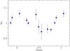 |
Fig. A.33 Variation with rotation phase of the average |
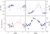 |
Fig. A.34 Mean longitudinal magnetic field (top left), crossover (bottom left), mean quadratic magnetic field (top right), and mean magnetic field modulus (bottom right) of the star HD 94660, against rotation phase. The symbols are as described at the beginning of Appendix A. |
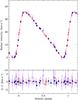 |
Fig. A.35 Upper panel: our radial velocity measurements for HD 94660 are plotted together with those of Bailey et al. (2015) against orbital phase. The solid curve corresponds to the orbital solution given in Table 12. The time T0 of periastron passage is adopted as phase origin. Bottom panel: plot of the differences O−C between the observed values of the radial velocity and the predicted values computed from the orbital solution. The dotted lines correspond to ± 1 rms deviation of the observational data about the orbital solution (dashed line). Filled squares represent the data from Bailey et al. and open triangles our CASPEC observations; all other symbols refer to our high-resolution spectra obtained with various instrumental configurations, as indicated in Table 3. |
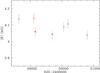 |
Fig. A.36 Mean magnetic field modulus of the star HD 110066, against heliocentric Julian date. The symbols are as described at the beginning of Appendix A. |
Romanyuk et al. (2014) state that their ⟨ Bz ⟩ data are incompatible with  . However, all their measurements but the most recent three have uncertainties about twice as large as ours, and also twice as large as the amplitude of the sinusoid that we fit to the longitudinal field values that we obtained. Since that amplitude is below the level of formal significance, we are led to suspect that the data of Romanyuk et al. (2014) are not precise enough to detect the variation. This suspicion is also borne out by consideration of their Fig. 4; the period shown in the latter,
  is definitely inconsistent with our determinations of the mean magnetic field modulus. On the other hand, the ⟨ Bz ⟩ measurements of Romanyuk et al. (2014) appear systematically shifted by about −200 G with respect to ours; such minor differences are not unusual between longitudinal field determinations from observations obtained with different telescopes and instruments.
The value Prot = 5.3832 d proposed by Wraight et al. (2012) on the basis of photometric data obtained with the STEREO satellites is not supported by our magnetic field data either.
The quadratic field shows no definite variation, which is not surprising, considering that the uncertainty of its determinations is large compared with the amplitudes observed for the variations of the longitudinal field and the field modulus. The value of ⟨ Bq ⟩ obtained by Mathys & Hubrig (2006) from the analysis of a sample of Fe i lines in a spectrum of HD 116114 recorded over a broader wavelength range and at higher resolution than our CASPEC spectra (7158 ± 190) G, is somewhat smaller than any of the values determined here, but is consistent with most of them within their respective uncertainties. Two of the six crossover values are significant at a level >3σ. While it is plausible that crossover due to stellar rotation is detected for a 276 period, the fact that all values of ⟨ Xz ⟩ derived here are negative (with one exception, which is not formally significant), albeit with a coverage gap between phases 0.3 and 0.8, and that no clear variation with the rotation period is observed, raises questions about the nature of the measured effect. This is further discussed in Sect. 5.3.
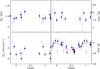 |
Fig. A.37 Mean longitudinal magnetic field (top left), crossover (bottom left), mean quadratic magnetic field (top right), and mean magnetic field modulus (bottom right) of the star HD 116114, against rotation phase. The symbols are as described at the beginning of Appendix A. |
The field moments determined from the CASPEC spectra are based on the analysis of a set of Fe i lines that show no equivalent width variation.
The variability of the radial velocity of HD 116114 was announced in Paper I and confirmed by Carrier et al. (2002), who suggested that the orbital period of this spectroscopic binary is of the order of 4000 days. This suggestion appears founded from inspection of Fig. A.38, where their data and ours are plotted together. This figure is a good illustration of the precision of the radial velocity measurements obtained from our high-resolution spectra, and of their consistency with those of Carrier et al.
A few years ago, Elkin et al. (2005a) announced the discovery of oscillations with a period of 21 min in HD 116114, making it the rapidly oscillating Ap (roAp) star with the longest pulsation period known at the time, and the most evolved one.
Appendix A.22: HD 116458
HD 116458 has already been extensively studied in our previous papers, both from high-resolution spectroscopy in natural light (Paper I; Mathys 1990; Mathys & Lanz 1992), and from spectropolarimetric observations (Mathys 1994, 1995a,b; Mathys & Hubrig 1997). Combining the data from those papers with the 11 new measurements of the mean longitudinal magnetic field presented here, we refined the determination of the value of the rotation period, Prot = (148.39 ± 0.33) d, which is used to compute the phases against which the measurements are plotted in Fig. A.39. The new ⟨ Bz ⟩ data have considerably smaller error bars than the old data, and they nicely line up along a cosine wave, with little scatter. The amplitude of the variation appears smaller than could have been suspected from the old, less precise measurements.
The mean magnetic field modulus and the mean quadratic field do not show any significant variability. The standard deviation of all our ⟨ B ⟩ data about their average, 4677 G, is only 31 G; in our sample, the field modulus measurements only show less scatter for HD 137949 and HD 177765. For the quadratic field, considering only the new measurements of this paper (which are considerably better than the old ones), the standard deviation of the data is 169 G, which is smaller than the average uncertainty of the individual determinations (211 G). The average of the new determinations of ⟨ Bq ⟩, 5252 G, is however somewhat larger than the value of 4716 G obtained by Mathys & Hubrig (2006) from analysis of a sample of 83 Fe ii lines observed at higher spectral resolution. But the Mathys & Hubrig (2006) value may somewhat underestimate the actual field strength, as can be inferred from the fact that it is not significantly larger than the field modulus.
As in other stars, the best-determined value of the crossover does not reach the threshold of significance, at 2.2σ. However, one notes that among the 11 new determinations of this field moment, all but one (which does not significantly differ from 0) are negative. Furthermore, these 11 data points appear to define a curve of variation of the crossover with the rotation period that is in phase quadrature with the variation of the longitudinal field. This is further discussed in Sect. 5.3.
No variability is observed for the equivalent widths of the Fe ii lines from which ⟨ Bz ⟩, ⟨ Xz ⟩ , and ⟨ Bq ⟩ are diagnosed.
HD 116458 is an SB1 whose orbit has first been determined by Dworetsky (1982). Our first attempt to combine our radial velocity measurements with those of this author led to a revised orbital solution about which the residuals O−C for the former still showed a low-amplitude variation with the orbital period. This appears to be due to the fact that the measurement errors of Dworetsky were underestimated, so that his data were given too large a weight in the combined data set. Dworetsky himself noted that the rms error derived from his orbital solution was “nearly three times the mean internal error” of his individual measurements. Adopting the former (1.7 km s-1) for the uncertainty of all his radial velocity values, rather than the (smaller) estimates quoted for each determination in Table I of his paper, we obtain an orbital solution in which the residuals no longer show any significant periodic variation. The elements given in Table 12 and the orbital curve shown in Fig. A.40 correspond to this solution. Not surprisingly, given that consideration of our data together with those of Dworetsky (1982) more than doubles the time interval covered by the measurements, our determination of the orbit represents a significant improvement, albeit fully compatible with the original solution by Dworetsky within the errors.
Appendix A.23: HD 119027
In Paper I, it was argued that the rotation period of the roAp star HD 119027 could plausibly be of the order of a few weeks, but its value remained elusive. The addition of a single magnetic field modulus measurement to the data of that paper (plotted with them in Fig. A.41) is insufficient to make any progress in its determination.
We present here the first measurements of the longitudinal field and the quadratic field of the star, which were obtained from analysis of a set of Fe i lines; both are well above the significance threshold. No significant crossover was detected in our single spectropolarimetric observation.
Romanyuk et al. (2014) also obtained a single measurement of the longitudinal field in this star. Both the value that they derived, ⟨ Bz ⟩ = 930 G, and our determination, ⟨ Bz ⟩ = 510 G, are positive. But we do not have enough information to decide whether the difference between those two values, which is formally very significant, reflects the variation that the stellar field underwent between the two observations, which took place 11 yr apart, or systematic effects resulting from the usage of different telescope and instrument combinations.
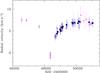 |
Fig. A.38 Our radial velocity measurements for HD 116114 are plotted together with those of Carrier et al. (2002) against heliocentric Julian date. Open triangles correspond to the Carrier et al. data and filled triangles to our CASPEC observations; all other symbols refer to our high-resolution spectra obtained with various instrumental configurations, as indicated in Table 3. |
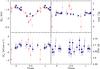 |
Fig. A.39 Mean longitudinal magnetic field (top left), crossover (bottom left), mean quadratic magnetic field (top right), and mean magnetic field modulus (bottom right) of the star HD 116458, against rotation phase. The symbols are as described at the beginning of Appendix A. |
Appendix A.24: HD 126515
The new determinations of the mean magnetic field modulus and the mean longitudinal magnetic field of HD 126515 (Preston’s star) agree well with the refined value of the rotation period derived in Paper I,  (see Fig. A.42). Their combination with our older data for these field moments allow their variation curves to be more precisely characterised. The strong anharmonicity of the ⟨ Bz ⟩ curve, mentioned in Paper I, is fully confirmed. The departure of the ⟨ B ⟩ curve from a single cosine wave is much less pronounced; the contribution of the harmonic is not visually compelling in Fig. A.42, but at 2.9σ, the second-order term of the fit is just below the threshold of formal significance. That is very unusual because, in general, the longitudinal field variation curves are very nearly sinusoidal even in those stars in which a strong anharmonicity of the field modulus variations is observed. The negative extremum of ⟨ Bz ⟩ coincides in phase with the maximum of ⟨ B ⟩.
The shape of the quadratic field variations is less well characterised, in particular because from phase 0.81 to phase 0.19, it is only constrained by older determinations, which are considerably less precise than those published in this paper. The anharmonicity of the ⟨ Bq ⟩ curve critically depends on the precision of the old measurements of this field moment; it cannot be regarded as definitely established.
We almost certainly detect crossover in this star; see the detailed discussion of Sect. 5.3. However, its variation with rotation phase is ill-defined, in part because over a large portion of the cycle (from phase ~0.8 to phase ~0.2), it is constrained only by the old, less precise measurements of Mathys (1995a) and Mathys & Hubrig (1997).
The large ratio between the extrema of ⟨ B ⟩ (1.7) indicates significant departure of the field geometry from a centred dipole. The asymmetry of the ⟨ Bz ⟩ variation curve reflects the lack of symmetry of the field about an axis passing through the centre of the star.
Preston (1970) had already reported the variability of the equivalent widths of the Fe lines in HD 126515. This variability is confirmed and more precisely characterised from consideration of the Fe ii lines from which ⟨ Bz ⟩, ⟨ Xz ⟩, and ⟨ Bq ⟩ are determined. As can be seen in Fig. A.43, the amplitude of variation of the equivalent widths of these lines is larger than in most other stars discussed in this paper. This has to be kept in mind in the interpretation of the magnetic field measurements. The lines are stronger close to the negative pole of the star (minimum of the field modulus).
Appendix A.25: HD 134214
The four new measurements of the mean magnetic field modulus of the roAp star HD 134214 presented here do not enable us to confirm or rule out the tentative value  of its rotation period proposed in Paper I. However, several other values of the period seem equally probable. This is why we prefer to plot our measurements against the Julian date in Fig. A.44. The standard deviation of our ⟨ B ⟩ determinations, 63 G, is larger than the precision that we expect for our measurements (compare e.g. with the standard deviations for HD 137949 or HD 177765). This suggests that the scatter of our data reflects actual variations, but until now their periodicity eludes determination. On the other hand, Adelman (2000a) confirmed that no photometric variations could be detected in this star, besides those caused by its pulsation.
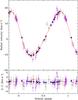 |
Fig. A.40 Upper panel: our radial velocity measurements for HD 116458 are plotted together with those of Dworetsky (1982) against orbital phase. The solid curve corresponds to the orbital solution given in Table 12. The time T0 of periastron passage is adopted as phase origin. Bottom panel: plot of the differences O−C between the observed values of the radial velocity and the predicted values computed from the orbital solution. The dotted lines correspond to ± 1 rms deviation of the observational data about the orbital solution (dashed line). Open triangles represent the data from Dworetsky and open squares our CASPEC observations; all other symbols refer to our high-resolution spectra obtained with various instrumental configurations, as indicated in Table 3. |
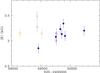 |
Fig. A.41 Mean magnetic field modulus of the star HD 119027, against heliocentric Julian date. The symbols are as described at the beginning of Appendix A. |
The magnetic field moments derived from our spectropolarimetric observations do not show any variability either; the equivalent widths of the Fe i lines on which their diagnosis is based appear constant as well. HD 134214 is one of the two stars of the sample for which the best precision is consistently achieved in the determination of ⟨ Bz ⟩. With error bars about five times smaller than those of Mathys & Hubrig (1997), we independently confirm the definite detection of a moderate longitudinal field in HD 134214 reported by Romanyuk et al. (2014). Our measurements, obtained between Januray 1996 and January 1998, show little, if any, variations of ⟨ Bz ⟩ around a mean value of ~−360 G. The difference with the values obtained between 1999 and 2007 by Romanyuk et al. (2014), which range from −700 to −900 G, is probably of instrumental origin.
The quadratic field of HD 134214 is about 1.3 times larger than the field modulus. No crossover is detected.
Appendix A.26: HD 137909
Since the publication of Paper I, a large number of measurements of the mean longitudinal magnetic field modulus of HD 137909 (β CrB) have been published by various groups, i.e. Hildebrandt et al. (2000), Wade et al. (2000b), and Leone & Catanzaro (2001). The latter authors, combining published data of various groups accumulated over more than 40 yr, confirm the adequacy of the value of the rotation period derived by Kurtz (1989),  . In particular, the revised value proposed by Bagnulo et al. (2000) does not represent a significant improvement over the latter.
All our data are plotted in Fig. A.45 against the phases computed using Kurtz’s ephemeris. The fairly large numbers of new measurements of the mean magnetic field modulus obtained with both AURELIE and the KPNO Coudé spectrograph (8 and 6, respectively) allow the systematic differences between the values of ⟨ B ⟩ obtained at the two sites to be better visualised. Unfortunately, a gap remains in the coverage of the KPNO data between phases 0.37 and 0.84, which leaves some ambiguity as to their exact nature. It seems inescapable, however, that as already suspected in Paper I, a somewhat different shape of the ⟨ B ⟩ variation curve is defined by the measurements from the two instruments. This indicates that caution is in order when interpreting the shapes of the variation curves in terms of the actual structure of the stellar magnetic fields; this is the case not only in HD 137909, but more generally in any star.
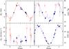 |
Fig. A.42 Mean longitudinal magnetic field (top left), crossover (bottom left), mean quadratic magnetic field (top right), and mean magnetic field modulus (bottom right) of the star HD 126515, against rotation phase. The symbols are as described at the beginning of Appendix A. |
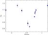 |
Fig. A.43 Variation with rotation phase of the average |
However, it appears unquestionable that the variation of the field modulus in HD 137909 has a significant degree of anharmonicity. Since we do not know how to handle the inconsistency between the OHP and KPNO data better, we fitted all of them together with a cosine wave and its first harmonic. By contrast, ⟨ Bz ⟩, for which we present here six new measurements, has a variation curve that shows no significant departure from a cosine wave. The introduction of the first harmonic in the ⟨ Bz ⟩ fit, driven by the behaviour of ⟨ B ⟩, does not in the least improve it. The anharmonic character of the crossover variation curve is more convincing to the eye but not formally significant, and one should note that it is, to a large extent, defined by the less precise old data points; the new determinations are not conclusive in this respect. The new quadratic field measurements do not show any significant variability (but they do not rule it out either); the old data points were reasonably represented by a cosine wave alone, but this cosine wave is inconsistent with the more precise determinations of this paper.
The new values of ⟨ Bz ⟩, ⟨ Xz ⟩ , and ⟨ Bq ⟩ presented here were derived from the analysis of a set of Fe i and Fe ii lines, for which no significant equivalent width variation is observed.
North et al. (1998) refined the determination of the orbital elements of HD 137909, which is an SB1, by combining their own radial velocity measurements with those of previous authors. Our radial velocity data are contemporaneous with theirs, and agree well with them (see Fig. A.46), but they do not set any additional constraint on the orbit. In addition, radial velocity oscillations, with a period of 16.21 min, were discovered in this star (Hatzes & Mkrtichian 2004).
Appendix A.27: HD 137949
The standard deviation of all our mean magnetic field modulus measurements of the roAp star HD 137949 (13 points from Paper I, and 7 new determinations reported here; see Fig. A.47) is only 23 G. Thus ⟨ B ⟩ has remained remarkably constant over the time span covered by our observations, 7.5 yr. This indicates that either the field modulus of this star does not vary at all, or its rotation period must be much longer than 7.5 yr.
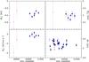 |
Fig. A.44 Mean longitudinal magnetic field (top left), crossover (bottom left), mean quadratic magnetic field (top right), and mean magnetic field modulus (bottom right) of the star HD 134214, against heliocentric Julian date. The symbols are as described at the beginning of Appendix A. |
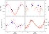 |
Fig. A.45 Mean longitudinal magnetic field (top left), crossover (bottom left), mean quadratic magnetic field (top right), and mean magnetic field modulus (bottom right) of the star HD 137909, against rotation phase. The symbols are as described at the beginning of Appendix A. |
Consideration of the other observables for which we have obtained measurements supports a long period. The equivalent widths of the Fe i lines used to diagnose the magnetic field in our CASPEC spectra do not show any definite variation. No crossover is detected; the formally most significant determination of this field moment, reaches the 2.7σ level, but none of the other exceed 1.2σ. The longitudinal field and quadratic field both appear constant over the time interval of more than 2 yr separating our first and most recent observations. As already mentioned in Paper I, however, different values of ⟨ Bz ⟩ have been obtained by various authors at different epochs (Babcock 1958; van den Heuvel 1971; Wolff 1975; Mathys & Hubrig 1997; Hubrig et al. 2004a). We gave arguments in Paper I supporting the view that no significant variation of ⟨ Bz ⟩ is definitely observed within any of those data sets taken in isolation. On the other hand, comparison between longitudinal field values determined by application of different diagnostic techniques to observations obtained with different telescope and instrument combinations is always subject to ambiguity owing to the possible existence of different systematic errors. Assuming that they can be neglected, we suggested in Paper I that ⟨ Bz ⟩ had been increasing monotonically since the time of the discovery of the magnetic field of HD 137949 by Babcock (1958).
A recent analysis of FORS longitudinal field data by Landstreet et al. (2014) seems to support that interpretation. However, this conclusion rests on the assumption that there are no major systematic differences between the ⟨ Bz ⟩ values derived from the low spectral resolution FORS observations and those of Paper I and of other studies based on high-resolution spectropolarimetry. The validity of this assumption is challenged by comparison of the measurements of Landstreet et al. (2014) with those of Romanyuk et al. (2014), which were published at almost the same time. In particular, Romanyuk et al. (2014) determined ⟨ Bz ⟩ = (1415 ± 70) G on HJD 2 452 333, while Landstreet et al. (2014) obtained ⟨ Bz ⟩ = (2689 ± 70) G and ⟨ Bz ⟩ = (2843 ± 64) G from two observations obtained with slightly different instrumental configurations on HJD 2 452 383. The difference of a factor of ~2 between those measurements performed by the two groups only 50 days apart represents a major inconsistency if the stellar rotation period is indeed of the order of decades. Furthermore, the value of ⟨ Bz ⟩ = (2146 ± 55) G derived by Hubrig et al. (2004a) through a separate analysis of the same FORS data strengthens the suspicion that, for HD 137949, FORS yields systematically higher longitudinal field values than other instruments.
By contrast, when combining the data of Romanyuk et al. (2014) with those of Mathys & Hubrig (1997) and of this paper, a coherent picture emerges in which the longitudinal field has passed through a minimum between 1998 and 2002, and which hints at a period of the order of 5300 days. To seek confirmation, we carried out a period search including the above-mentioned data sets and the earlier measurements of Babcock (1958), van den Heuvel (1971), and Wolff (1975). A peek stands out rather clearly in the periodogram, corresponding to Prot = 5195 d. An error bar cannot be associated with that value given the uncertainty of the possible existence of systematic differences between ⟨ Bz ⟩ measurements obtained with different instrumental configurations (in particular, between the determinations obtained since 1992 using CCD observations and those from 1975 and before that relied on photographic plates). But consideration of Fig. A.48, where the longitudinal field variations are plotted as a function of the rotation phase computed using the proposed value of the period, strengthens our confidence that this value is essentially correct, especially in view of its consistency with all the data obtained since 1992.
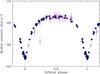 |
Fig. A.46 Our radial velocity measurements for HD 137909 are plotted together with those of North et al. (1998) against the orbital phase computed using the (final) orbital elements of these authors. Dots correspond to the North et al. data and open triangles to our CASPEC observations; all other symbols refer to our high-resolution spectra obtained with various instrumental configurations, as indicated in Table 3. |
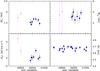 |
Fig. A.47 Mean longitudinal magnetic field (top left), crossover (bottom left), mean quadratic magnetic field (top right), and mean magnetic field modulus (bottom right) of the star HD 137949, against heliocentric Julian date. The symbols are as described at the beginning of Appendix A. |
Despite their overall consistency with the measurements of Romanyuk et al. (2014), our data are difficult to reconcile with their suggested short period,  . In particular, with that value of the period, the lowest value of the longitudinal field that we derive, ⟨ Bz ⟩ = 1425 G, on HJD 2 449 916, would be found close to the phase of maximum of ⟨ Bz ⟩. The measurements of Mathys & Hubrig (1997) would also be significantly discrepant. Overall, the long period Prot = 5195 d (or 14.2 yr) represents a much better match to the combination of our data and of those of Romanyuk et al. (2014).
The derived values of ⟨ Bq ⟩ are marginally smaller than those of ⟨ B ⟩ (by about 50 G, in average). This non-physical difference is not formally significant, but it probably indicates that our quadratic field determinations for this star are slightly underestimated. They are marginally smaller than the value obtained by Mathys & Hubrig (2006) from analysis of Fe i line profiles in a contemporaneous spectrum of higher resolution covering a broader wavelength range.
Our radial velocity data and those of Carrier et al. (2002) are shown against Julian date in Fig. A.49. The measurements that we obtained from our high-resolution spectra recorded in natural light (all with the CES) definitely do not show the scatter reported by Carrier et al.; their standard deviation is only 0.22 km s-1. Our CASPEC data show somewhat more scatter, but not more than expected from their more limited accuracy. The main difference between our determinations and those of Carrier et al. is that ours rely exclusively on Fe lines, while theirs use lines of a large number of chemical elements. This is consistent with their tentative interpretation that the radial velocity variations that they detect are due to spots coming in out and view as the star rotates, since typically Fe is fairly uniformly distributed on the surface of Ap stars, while other elements tend to show larger inhomogeneities. But this interpretation cannot be reconciled with the length of the rotation period that is inferred from the magnetic field variations. Also, the non-negligible apparent v sini mentioned by Carrier et al. is more probably reflecting the magnetic broadening of the spectral lines. An alternative explanation to the different behaviour of our radial velocity measurements and those of Carrier et al. is that the scatter of the latter (and also the variability of the width of the correlation dip) is caused by pulsation. This is made plausible by the fact that, in this star (as in many roAp stars), the amplitude of the radial velocity variations due to pulsation is considerably smaller for Fe than for a number of other elements (Kurtz et al. 2005). However the magnitude of the scatter of the Carrier et al. data seems too large with respect to the amplitudes observed by Kurtz et al. in individual lines, especially if one takes into account the fact that, in the Carrier et al. case, the signal is diluted by the lines that show lower amplitude variations, or no variation at all, and (probably) by the fact that the integration time represents a non-negligible fraction of the period of the stellar pulsation. One would have to assume that the pulsation amplitude varies with time, which is actually observed in other stars and, hence, cannot be ruled out. But it will need to be established by future observations.
Appendix A.28: HD 142070
The value of the rotation period of HD 142070 published in Paper I was erroneous because the Julian dates of two of the magnetic field modulus measurements were wrong by one day. The dates appearing in Table 4 of Paper I are correct, but the correction took place after the period was determined. With the correct dates, and the two new ⟨ B ⟩ determinations presented here, a revised value of the period is obtained, Prot = (3.3718 ± 0.0011) d. This value is in excellent agreement with the value derived by Adelman (2001) from the analysis of photometric data, Prot = (3.37189 ± 0.00007) d. Although the latter is formally more accurate, in what follows we use the value of the period that we obtained because the variation of the magnetic field is much better defined; that is, its amplitude is much larger with respect to the individual measurement errors.
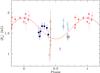 |
Fig. A.48 Mean longitudinal magnetic field of the star HD 137949 against rotation phase assuming Prot = 5195 d (see text). The various symbols correspond to measurements by different authors: the open triangle indicates Babcock (1958); open squares indicate van den Heuvel (1971); open circles indicate Wolff (1975); filled triangles indicate Mathys & Hubrig (1997); dots indicate this paper; and filled squares indicate Romanyuk et al. (2014). |
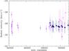 |
Fig. A.49 Our radial velocity measurements for HD 137949 are plotted together with those of Carrier et al. (2002) against heliocentric Julian date. Open triangles correspond to the Carrier et al. data and filled triangles to our CASPEC observations; all other symbols refer to our high-resolution spectra obtained with various instrumental configurations, as indicated in Table 3. |
Romanyuk et al. (2014) also report that their longitudinal field measurements are compatible with  . The ⟨ Bz ⟩ values that they derive appear to be systematically shifted by ~−150 G with respect to ours, as a result of the usage of different instruments and line samples for their determination.
In Paper I we inferred from consideration of the fairly short rotation period of HD 142070 and of its low v sini that the inclination of its rotation axis over the line of sight cannot exceed 8°. It is particularly remarkable that, in spite of this low inclination, all field moments but the quadratic field show very well-defined variations with significant amplitude (see Fig. A.50). The longitudinal field reverses its sign: as the star rotates, both magnetic poles come alternatively into view. This implies that the magnetic axis must be very nearly perpendicular to the rotation axis. The crossover is large as well. The variation curve of ⟨ B ⟩ is strongly anharmonic, although the scarcity of measurements between phases 0.6 and 0.0 implies that its shape is not fully constrained. The variation curves of ⟨ Bz ⟩ and ⟨ Xz ⟩ do not significantly depart from cosine waves. They are in phase quadrature with each other, within the limits of the precision of the phase origin determinations. The positive extremum of ⟨ Bz ⟩ coincides in phase with the primary maximum of ⟨ B ⟩; to the extent that the phase of the secondary maximum of ⟨ B ⟩ is constrained, it seems to occur close to the negative extremum of ⟨ Bz ⟩. Variations of the quadratic field are not definitely detected. As in several other stars, this field moment appears to be somewhat underestimated, since it tends at most phases to be marginally smaller than the field modulus.
The longitudinal field, the crossover and quadratic field were determined through analysis of a set of Fe ii lines. The equivalent widths of these lines do not appear to be variable.
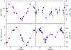 |
Fig. A.50 Mean longitudinal magnetic field (top left), crossover (bottom left), mean quadratic magnetic field (top right), and mean magnetic field modulus (bottom right) of the star HD 142070, against rotation phase. The symbols are as described at the beginning of Appendix A. |
In Paper I, we had found that the radial velocity of HD 142070 is variable. Carrier et al. (2002) confirmed this discovery. Their measurements are plotted together with ours in Fig. A.51. The two sets are contemporaneous and there is good agreement between them. Our data bracket the radial velocity minimum more narrowly than the data of Carrier et al., and accordingly our data define somewhat better the shape of the radial velocity curve around that phase. But our data do not provide new constraints about the orbital period, and the conclusion by Carrier et al. that it must be of the order of 2500 d or longer remains valid.
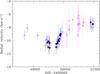 |
Fig. A.51 Our radial velocity measurements for HD 142070 are plotted together with those of Carrier et al. (2002) against heliocentric Julian date. Open triangles correspond to the Carrier et al. data and filled triangles to our CASPEC observations; all other symbols refer to our high-resolution spectra obtained with various instrumental configurations, as indicated in Table 3. |
Appendix A.29: HD 144897
As for HD 142070, the value of the rotation period derived in Paper I for HD 144987 is affected by a one-day error in the Julian dates of two of the mean magnetic field modulus measurements. The dates appearing in Table 4 of Paper I are correct, but the correction took place after the period was determined. After correction of these two dates, and addition of the two new ⟨ B ⟩ measurements reported in this paper, a revised value of the period is obtained, Prot = (48.57 ± 0.15) d.
This value also matches the variations of the other field moments, as can be seen in Fig. A.52, where it is used to compute the phases. While a cosine wave represents an excellent approximation to the behaviour of the field modulus, the addition of the first harmonic considerably improves the quality of the fits to the variation curves of the longitudinal field and quadratic field (for which the data set includes one observation of Mathys & Hubrig 1997), both visually and from consideration of χ2/ν, even though the fitted amplitudes of the harmonic are just below the limit of formal significance.
Only 1 of the 13 determinations of the crossover is significantly non-zero, but it is intriguing that all but 2 yield positive values. Furthermore if the measurement of Mathys & Hubrig (1997), which may be of lower quality as in a number of other stars, is discarded, a fit by a cosine wave with twice the rotation frequency (that is, a first harmonic alone) appears significant with a computed variation amplitude at the 4.4σ level. The parameters appearing in Table 10 and the ⟨ Xz ⟩ curve plotted in Fig. A.52 correspond to this case. This is further discussed in Sect. 5.3.
The longitudinal field is always positive. The fact that its primary minimum very nearly coincides in phase with the maxima of the field modulus and of the quadratic field indicates that its structure must depart significantly from a centred dipole, as already suspected from the probable anharmonicity of the variation curves of several field moments.
The lines of Fe ii, which were used to diagnose the magnetic field from the CASPEC spectra, do not show any significant equivalent width variation over the stellar rotation period.
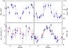 |
Fig. A.52 Mean longitudinal magnetic field (top left), crossover (bottom left), mean quadratic magnetic field (top right), and mean magnetic field modulus (bottom right) of the star HD 144897, against rotation phase. The symbols are as described at the beginning of Appendix A. |
Figure A.53 shows that the radial velocity of HD 144897 has been slowly decreasing from the time of our first observation of the star until the seasonal observability gap of end of 1994 and early 1995; since then until September 1998, it appears to have been increasing monotonically (even though the larger uncertainties of the CASPEC measurements tend to confuse the picture). The overall amplitude of the variations observed until now is of the order of 3 km s-1: the star appears to be a spectroscopic binary with an orbital period in excess of six years. To the best of our knowledge, the binarity of HD 144897 is reported here for the first time.
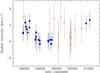 |
Fig. A.53 Our radial velocity measurements for HD 144897 are plotted against heliocentric Julian date. Open squares correspond to our CASPEC observations; all other symbols refer to our high-resolution spectra obtained with various instrumental configurations, as indicated in Table 3. |
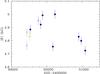 |
Fig. A.54 Mean magnetic field modulus of the star HD 150562, against heliocentric Julian date. The symbols are as described at the beginning of Appendix A. |
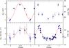 |
Fig. A.55 Mean longitudinal magnetic field (top left), crossover (bottom left), mean quadratic magnetic field (top right), and mean magnetic field modulus (bottom right) of the star HDE 318107, against rotation phase. The symbols are as described at the beginning of Appendix A. |
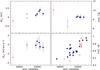 |
Fig. A.56 Mean longitudinal magnetic field (top left), crossover (bottom left), mean quadratic magnetic field (top right), and mean magnetic field modulus (bottom right) of the star HD 165474, against heliocentric Julian date. The symbols are as described at the beginning of Appendix A. |
Appendix A.30: HD 150562
The presence of magnetically resolved split lines in the spectrum of the little-studied roAp star HD 150562 was announced in Paper I. The seven ⟨ B ⟩ measurements of this paper are plotted together with five new determinations in Fig. A.54. All data points but one convincingly indicate that the rotation period must be longer than the time range covered by our observations, which is 4.5 yr. Most likely, the deviating measurement, obtained on HJD 2450171.802, is wrong and it should be ignored, although we cannot clearly identify a reason for its bad quality; an unrecognised cosmic ray event in one of the components of the line Fe ii λ 6149 seems the most plausible source of error.
The maximum of the field modulus of HD 150562 appears close to 5.0 kG. Only one spectropolarimetric observation of the star could be obtained, revealing a positive longitudinal field and a quadratic field that must have been of the order of 10% greater than the field modulus around the same phase. No crossover is detected, which is consistent with a rotation period of several years. The available observations are insufficient to draw definite conclusions about the possible variability of the radial velocity, or of the equivalent widths of the Fe i lines that were used for determination of the longitudinal field, the crossover, and the quadratic field.
Appendix A.31: HDE 318107
A detailed study of the variations of HDE 318107 was carried out by Manfroid & Mathys (2000), who succeeded in establishing the value of the rotation period of the star, Prot = (9.7085 ± 0.0021) d. This value was subsequently refined to Prot = (9.7088 ± 0.0007) d by Bailey et al. (2011), from consideration of additional magnetic field measurements. This improved value is used here.
The study of Manfroid & Mathys (2000) was based in part on a revision of the values of the mean magnetic field modulus derived in Paper I, as well as on the four new measurements presented here. The revision of part of the Paper I data was carried out in an attempt to measure the line Fe ii λ 6149 in a more uniform manner at all phases, which is an endeavour complicated by its variable strong blending, as well as for some observations, by the fairly low S/N of the spectra. The revised measurements are included in Table 5.
All the measurements of the mean magnetic field modulus, as well as the values of the other field moments derived from spectropolarimetric observations (including one set from Mathys & Hubrig 1997) are plotted against rotation phase in Fig. A.55. The variation curve of ⟨ B ⟩ is definitely anharmonic with a broad, almost flat minimum over about half of the rotation period. The shapes of the variation curves of the other field moments are not well defined owing to the small number of data points. The longitudinal field appears to be always positive with a phase of minimum close to the phase of maximum of the field modulus. As already pointed out for other stars, this is indicative of a field structure significantly departing from a centred dipole.
None of the individual crossover determinations are significant (there is only one above the 1σ level), but when plotted against phase they seem to line up along a cosine wave, and the amplitude coefficient of a fit by such a wave is formally significant, just at the 3σ level. The multiple correlation coefficient is also rather high, R = 0.87.
The quadratic field is nearly constant over the rotation period with the exception of one measurement being considerably higher than the others. The most likely explanation is that this determination is spurious (without obvious reason, though), but the proximity of this point to the phase of maximum of the field modulus, and the steep variation of the latter around this phase do not allow one to rule out the reality of the considered ⟨ Bq ⟩ value.
The lines of Fe ii, from which ⟨ Bz ⟩, ⟨ Xz ⟩ , and ⟨ Bq ⟩ are determined do not show any definite equivalent width variations.
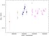 |
Fig. A.57 Mean longitudinal magnetic field of the star HD 165474 against heliocentric Julian date. The different symbols correspond to measurements by different authors: the filled square indicates Mathys (1994); open squares indicate Mathys & Hubrig (1997); dots indicate this paper; and filled triangles indicate Romanyuk et al. (2014). |
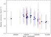 |
Fig. A.58 Our radial velocity measurements for HD 165474 are plotted against the heliocentric Julian date. All symbols refer to our high-resolution spectra obtained with various instrumental configurations, as indicated in Table 3. |
Appendix A.32: HD 165474
The tentative value of 254065 d proposed in Paper I for the rotation period of HD 165474, which more recently seemed borne out by independent measurements of Nielsen & Wahlgren (2002), is not confirmed by the 14 new measurements of its mean magnetic field modulus that are reported here, and no other short period emerges from the analysis of the whole set of ⟨ B ⟩ data. When all our measurements of this field moment are plotted against the Julian date (Fig. A.56), a slow monotonic increase is clearly seen, from our first point to our last one, indicative of a period considerably longer than the time interval separating them, of nine years. The evidence for a long period becomes even stronger if one allows for the existence of a systematic difference of the ⟨ B ⟩ values derived from AURELIE data with respect to those measured in spectra recorded with other instruments, as observed in a number of stars.
Even after taking that shift into account, the scatter of the individual measurements about a smooth variation curve is somewhat higher than would be expected from their adopted uncertainty. There is no obvious reason to suspect that the latter has been underestimated: the star is fairly bright, so that almost all spectra have high S/N; the components of the Fe ii λ 6149 line are well resolved, to such an extent that the line goes back up all the way to the continuum between them (HD 165474 is one of the very few stars where this is observed); their profiles are very regular and clean; and, in particular, there is no hint at all of the blend that hampers the measurement of the blue component in many other stars. The case is somewhat similar to that of HD 55719. For the time being we have no explanation for the higher than expected scatter of the individual ⟨ B ⟩ determinations about a smooth variation curve. This, however, does not question the reality of the variation. From the first to the last observation, the field modulus has increased by approximately 500 G, while once the AURELIE measurements have been shifted to make them consistent with the data obtained with other instruments, the rms of the points about a smooth variation trend is only of the order of 100 G.
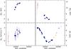 |
Fig. A.59 Mean longitudinal magnetic field (top left), crossover (bottom left), mean quadratic magnetic field (top right), and mean magnetic field modulus (bottom right) of the star HD 166473, against heliocentric Julian date. A diamond is used to represent the measurement of Mathys et al. (2007) obtained with the UVES spectrograph at Unit Telescope 2 of ESO’s Very Large Telescope. All other additional measurements of these authors are based on observations performed with instrumental configurations similar to those used for the present study; the same symbols are used to identify them as in the rest of this paper (see beginning of Appendix A. |
Several other arguments support the view that the rotation period of HD 165474 is long. With the variation trend observed in the data discussed here, it is not implausible that, at a later time, the field modulus may have reached a value close to the 7.2 kG value determined by Preston (1971) from the spectrum from which he discovered resolved magnetically split lines in the star. Nielsen & Wahlgren (2002) did not publish their individual ⟨ B ⟩ measurements, from spectra recorded with the SOFIN spectrograph at the Nordic Optical Telescope, but one can see from their Fig. 8 that they are all concentrated around a mean value of 6.6 kG. They were all obtained in a ten night interval centred on HJD 2 451 769, that is, a little more than two years after our last measurement. If there is no systematic shift between the data from Nielsen & Wahlgren and our data (which should not be taken for granted), their combination suggests that the field modulus of HD 165474 may have been through a maximum during 1999, and from then started to decrease with a significantly steeper slope than it had increased between 1989 and 1998. However, this will have to be confirmed because of the uncertain consistency of measurements obtained with different instruments.
None of the individual determinations of ⟨ Bz ⟩ presented here yield formally significant non-zero values. The older measurements of Mathys (1994) and Mathys & Hubrig (1997) did not yield any definite detection either. The corresponding 3σ upper limits of the longitudinal field range from 240 G to 450 G (except for the measurement performed by Mathys (1994) of a specrtrum obtained in 1988, which is less precise). The more recent ⟨ Bz ⟩ measurements of Romanyuk et al. (2014) have smaller error bars, and for 13 of them (i.e. a little more than half), a formally significant detection (at the 3σ level) is achieved.
The tentative value of the period proposed by Romanyuk et al. (2014),  , is definitely ruled out by our mean field modulus data. As a matter of fact, the scatter of the ⟨ Bz ⟩ values obtained by those authors is mostly consistent with the error bars; the occurrence of variations cannot be firmly established from consideration of their data set alone. We plotted their measurements together with ours against observation dates in Fig. A.57. Even allowing for possible systematic differences between ⟨ Bz ⟩ values derived from observations with different telescopes and instruments, the trend seen in this figure is consistent with the slow variability of the field over a very long period that we inferred from consideration of the field modulus.
Moreover, Babcock (1958) had measured a longitudinal field of 900 G in a spectrum recorded in 1957. The difference between this value and the more recent data shown in Fig. A.57 strengthens the argument favouring a long period.
This argument is also consistent with the fact that no crossover is detected and with the behaviour of the quadratic field. The determinations of the quadratic field presented in this paper, which are much more reliable than those of previous work, show it to be remarkably constant over the time interval April 1995–June 1997. The ratio between it and contemporaneous values of ⟨ B ⟩ is of the order of 1.25. This suggests that, unless the field structure is unusually tangled, a sizeable mean longitudinal field must be observable over a significant fraction of the rotation period. This in turn represents additional evidence that the rotation period of HD 165474 is very long, probably of the order of several decades. If, as hypothesised above, the value reported by Preston (1971) was close to the maximum of ⟨ B ⟩ and the star went through another maximum in 1999, it is not implausible that these two maxima may correspond to consecutive cycles, so that the rotation period may be of the order of the ~30 yr elapsed between them.
Not surprisingly, if the period is very long, no variations of equivalent widths of the Fe i and Fe ii lines used for diagnosis of the magnetic field from CASPEC data are observed over the 2.2 y time interval covered by them. This does not set any strong constraints on the distribution of the element on the surface of HD 165474.
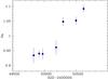 |
Fig. A.60 Variation with time of the average |
Figure A.58 shows that the radial velocity of HD 165474 has been decreasing very slowly from June 1992 (third data point from the left) to June 1998 (last point on the right). Over this six year time interval, the total amplitude of the radial velocity variation has barely reached 1 km s-1. The figure only shows the measurements performed on the high-resolution spectra recorded in natural light. The CASPEC data are not included because their larger uncertainties tend to blur the picture on visual inspection; but they are fully consistent with the above-described variation. The fact that such a minute progressive variation can be followed over a time span of six years, from analysis of data obtained with various instrumental configurations at different telescopes, demonstrates a remarkable stability and mutual consistency of these systems. In particular, the exceedingly small scatter about a smooth trend of the measurements obtained with the ESO Coudé Auxiliary Telescope and the Long Camera of the Coudé Echelle Spectrograph is a testimony to the exquisite performance of this instrumental configuration. However, the two data points obtained before June 1992 are insufficient to characterise the behaviour of HD 165474 before that time. It is not implausible that its radial velocity went through a maximum shortly before or around June 1992, but one cannot rule out either the possibility that the slow decrease seen later had started much earlier, and that the two pre-June 1992 measurements are just unfortunate outliers. In any event, it appears unquestionable that the star is a spectroscopic binary with an orbital period considerably longer than six years. HD 165474 has a visual companion, HD 165475, which is a fast rotating, superficially normal A star, located approximately 5′′ apart. It is unclear if they are physically related, and if so, whether the observed radial velocity variation corresponds to the orbit of the visual binary, or if it is caused by another, unseen component, which had not been detected before.
Appendix A.33: HD 166473
Ten new measurements of the mean magnetic field modulus of the roAp star HD 166473 are presented here, showing that it went through a minimum, of the order of 5.7 kG, between March and September 1997. This can be seen in Fig. A.59, where more recent measurements (Mathys et al. 2007) are also plotted, suggesting that the rotation period may be close to ten years, although this cannot be regarded as definitely established. In particular, the most recent value is 250 G higher than the first value, which is a formally significant difference.
In addition, seven determinations of ⟨ Bz ⟩, ⟨ Xz ⟩ , and ⟨ Bq ⟩ were obtained, which complement earlier measurements of Mathys & Hubrig (1997), showing in particular that the longitudinal field reverses its polarity, hence that both magnetic poles of the star come into view as it rotates.
Mathys et al. (2007) have discussed in detail the variations of all four field moments. We point out a couple of remarkable features here. The amplitude of variation of ⟨ B ⟩ is larger than in most stars with a ratio of 1.55 between the highest and lowest values determined from the observations obtained until now. On the other hand, the ratio between the quadratic field and the field modulus is found to be of the order of 1.00 around minimum and 1.25 around maximum. The latter value, however, may be affected by a large uncertainty, owing to the lower quality of the quadratic field determinations of Mathys & Hubrig (1997).
The equivalent widths of the Fe i lines, from which the longitudinal field, the crossover, and the quadratic field are determined, are definitely variable. This is illustrated in Fig. A.60, where the average is plotted against Julian date. The number of observations is insufficient to characterise the shape of the variation, but its extrema do not seem to coincide with those of the field modulus. In any case, one should bear in mind that the magnetic field moments involve a weighting by the inhomogeneous distribution of Fe i over the stellar surface.
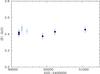 |
Fig. A.61 Mean magnetic field modulus of the star HD 177765, against heliocentric Julian date. The symbols are as described at the beginning of Appendix A. |
Appendix A.34: HD 177765
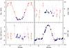 |
Fig. A.62 Mean longitudinal magnetic field (top left), crossover (bottom left), mean quadratic magnetic field (top right), and mean magnetic field modulus (bottom right) of the star HD 187474, against rotation phase. The symbols are as described at the beginning of Appendix A. |
The two new values of the mean magnetic field modulus of HD 177765 presented here do not significantly differ from those of Paper I. We have now obtained a total of eight measurements of this star, between August 1993 and September 1998 (see Fig. A.61), and their standard deviation about their mean is only 17 G. This is the smallest standard deviation derived for any of the stars studied in this paper. It must be very close to the ultimate precision achievable in our determinations of ⟨ B ⟩. As far as the star itself is concerned, the total lack of detectable variations most likely indicates that its rotation period is much longer than the time span over which it has been observed so far, which is five years. The recent measurement of a significantly higher mean field modulus, ⟨ B ⟩ = 3550 G, in a spectrum obtained in June 2010 by Alentiev et al. (2012) fully supports this view. It is very possible that HD 177765 may have a rotation period exceeding the time interval, 17 yr, between our first ⟨ B ⟩ measurement and the recent observation by Alentiev et al. These authors also reported the detection of rapid oscillations in this star with the longest pulsation period known so far for an roAp star.
We did not obtain any spectropolarimetric observation of HD 177765, for which no measurement of the longitudinal field was found in the literature.
Appendix A.35: HD 187474
The shape of the curve of variation of the mean magnetic field modulus of HD 187474 between phases of 0.36 and 0.86, which was left mostly unconstrained (but for one data point) in Paper I, is now fully characterised thanks to 12 new measurements (Fig. A.62). This field moment reaches its maximum (~6.3 kG) close to phase 0.47. This very nearly coincides with the phase of negative extremum of ⟨ Bz ⟩. The negative part of the variation curve of the latter is now fully characterised by our measurements, that is, by a set of data that are all obtained with the same instrument (although with different configurations). This curve shows a small, but formally significant (at the 3σ level), degree of anharmonicity with a variation that is somewhat steeper about the positive extremum than about the negative extremum, but no significant departure from mirror symmetry about the phases of the two extrema. This behaviour contrasts with that of the field modulus, which has a broad, almost flat minimum around the phase of ⟨ Bz ⟩ positive extremum, and a sharp maximum close to the phase of ⟨ Bz ⟩ negative extremum. The ⟨ B ⟩ variation is not as symmetric as that of ⟨ Bz ⟩, but the departure from symmetry is small, so that contrary to other stars, the magnetic structure may plausibly be (almost) symmetric about an axis passing through the stellar centre.
The behaviour of the quadratic field is ill-defined because earlier determinations (revised values of the measurements of Mathys 1995b, and especially data from Mathys & Hubrig 1997, obtained by application of Eq. (14) rather than the more realistic Eq. (9)) are considerably less accurate than those presented here. The latter hardly show any hint of variation, but this is mostly inconclusive because of their limited phase coverage. The ratio between ⟨ Bq ⟩ and ⟨ B ⟩ is of the order of 1.2 or greater, while the ratio between the maximum and minimum of the field modulus, 1.27, is close to the expected value for a centred dipole. The shape of the field modulus variation however indicates that the actual field structure does show non-negligible deviations from the latter.
None of the individual values of the crossover depart significantly from 0, as can be expected for a rotation period of 2345 d. Yet, it is intriguing that all but one of the nine new determinations of this paper yield marginally negative values; the larger uncertainties of older measurements (Mathys 1995a; Mathys & Hubrig 1997) make them unsuitable to test whether this effect is real, or purely coincidental. This is further discussed in Sect. 5.3
In the interpretation of the behaviour of the various field moments, one should keep in mind that the lines of Fe ii, from which they are derived, show significant equivalent width variations over the stellar rotation period. This is illustrated in Fig. A.63, where the equivalent width parameter is plotted against phase, for the spectropolarimetric observations of Mathys (1991, open circles) and of the present paper (dots). The two samples are distinguished because the definition of is such that its values are not a priori consistent between sets of observations covering different parts of the rotation cycle. Fortuitously, in the present case, the phase distributions of the two subsamples of observations under consideration are such that the sets of values of defined for each of these subsamples happen to be fairly consistent with each other. Figure A.63 show a double wave variation of the equivalent widths of the Fe ii lines in HD 187474 over its rotation period with maxima close to phases 0 and 0.5 and minima near phases 0.25 and 0.75. This is consistent with the results of the Strasser et al. (2001) study of the abundance distribution over the surface of the star, which shows some concentration of Fe around both magnetic poles.
HD 187474 is a spectroscopic binary for which Leeman (1964) derived an approximate value of the orbital period, Porb = 690 d (shorter than the rotation period of the Ap component) and quoted preliminary orbital elements derived by Miss Sylvia Burd from the analysis of 33 spectra obtained by Babcock. Here we combine 50 unpublished radial velocity measurements of Babcock (priv. comm.) with our data to determine a first complete orbital solution, based on data spanning a time interval of 42 yr. Its parameters are reported in Table 12 and the corresponding fit is shown in Fig. A.64.
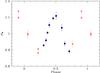 |
Fig. A.63 Variation with rotation phase of the average |
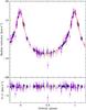 |
Fig. A.64 Upper panel: our radial velocity measurements for HD 187474 are plotted together with those of Babcock (priv. comm.) against orbital phase. The solid curve corresponds to the orbital solution given in Table 12. The time T0 of periastron passage is adopted as phase origin. Bottom panel: plot of the differences O−C between the observed values of the radial velocity and the predicted values computed from the orbital solution. The dotted lines correspond to ± 1 rms deviation of the observational data about the orbital solution (dashed line). Open triangles represent the data from Babcock and open squares our CASPEC observations; all other symbols refer to our high-resolution spectra obtained with various instrumental configurations, as indicated in Table 3. |
Appendix A.36: HD 188041
Among the stars discussed in this paper, HD 188041 is one of those showing the highest line density in the spectral range covered by the CASPEC spectra. Accordingly, virtually all lines that could be used for determination of the longitudinal field, the crossover, and the quadratic field, show some degree of blending. This makes their measurements difficult and increases the uncertainty of the derived field moments. However, the combination of the two new ⟨ Bz ⟩ values obtained here with the earlier data of Mathys (1994) and Mathys & Hubrig (1997) definitely confirms the existence of a systematic difference between the longitudinal field measurements of this star from CASPEC spectra and the earlier determinations of Babcock (1954, 1958), as already suggested by Fig. 35 of Mathys (1991). In order to bring both data sets in coincidence, a shift of −400 G has been applied to the CASPEC values, which are less numerous. The resulting combined data set is shown in the upper left panel of Fig. A.65, where it is plotted against the rotation phase corresponding to the value Prot = (223.78 ± 0.10) d of the period. This value, which we derived from the same data set, is in excellent agreement with the values obtained by Mikulášek et al. (2003) from photometric data of various origins (Prot = 223.826 ± 0.040 d) and from combination of the magnetic data of Babcock (1954, 1958), Wolff (1969b), and Mathys (1991; Prot = 223.78 ± 0.30 d). We did not include the Wolff (1969b) data in our analysis because of their rather large scatter and because the ⟨ Bz ⟩ determinations of the Hawaii group for many stars show unexplained discrepancies with the measurements by Babcock (and ours, which are mostly consistent with those of Babcock). Moreover, the values published by Mathys (1991) are superseded by the results of the revised analysis of Mathys (1994). The fit parameters appearing in Table 9 have also been computed for the whole data set shown in Fig. A.65. However, one of the measurements of Mathys & Hubrig (1997), on JD 2 448 782, has been discarded, on account of its abnormally large discrepancy with the other points. We have adopted the same phase origin as Wolff (1969b), even though it is now seen to be slightly shifted with respect to the minimum of ⟨ Bz ⟩.
The diagnostic lines measured in our CASPEC spectra, which belong to Fe i and Fe ii, are stronger close to the phase of maximum of the longitudinal field, and weaker around its phase of minimum, as already pointed out by Wolff (1969a). The ⟨ Bz ⟩ data therefore represent the convolution of the actual distribution of the line-of-sight component of the magnetic field on the stellar surface with the Fe inhomogeneities, which however do not appear very large.
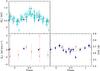 |
Fig. A.65 Mean longitudinal magnetic field (top left), crossover (bottom left), and mean magnetic field modulus (bottom right) of the star HD 188041, against rotation phase. The longitudinal field measurements of the present paper and those of Mathys (1994) and Mathys & Hubrig (1997) have been arbitrarily shifted by −400 G for consistency with the more numerous data of Babcock (1954, 1958) (asterisks). Except for the latter, the symbols are as described at the beginning of Appendix A. The mean quadratic field could not be determined in this star (see text for details). |
No significant crossover is detected. The quadratic field is also below the detection limit: the values derived from the two CASPEC spectra analysed here do not significantly differ from 0, with values of σq of 1.9 and 2.1 kG. In our previous studies (Mathys 1995b; Mathys & Hubrig 1997), application of Eq. (14) to our observations of this star yielded non-physical, negative values of a2. This is the only star of the present sample for which the quadratic field could not be determined at any phase because it is too small.
This is consistent with the fairly weak mean magnetic field modulus observed in HD 188041. The variations of the latter have a very small amplitude: the fitted curve has an amplitude below the threshold of formal significance, even though it almost certainly reflects real variations. In particular, we note the fairly good phase coincidence between the phases of extrema of ⟨ Bz ⟩ and ⟨ B ⟩; if the variations of the latter are real, the quasi-coincidence of its maximum with the minimum of ⟨ Bz ⟩ is indicative of departure of the field structure from a centred dipole. The three new measurements of the field modulus presented here are consistent with those of Paper I, but do not otherwise bring much progress in the knowledge of the magnetic field of HD 188041.
Our measurements of the radial velocity of the star show no significant variability, and they are in excellent agreement with those of Carrier et al. (2002).
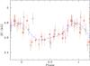 |
Fig. A.66 Mean magnetic field modulus of the star HD 192678, against rotation phase. The AURELIE data have been shifted by −142 G. The symbols are as described at the beginning of Appendix A. |
Appendix A.37: HD 192678
The magnetic field of HD 192678 has been studied in detail by Wade et al. (1996a). The value of the rotation period adopted by these authors (Prot = (6.4186 ± 0.002) d) has recently been refined by Adelman (2006) using photometric data. This new value, Prot = (6.4193 ± 0.0003) d, is used here to phase our observations.
As mentioned in Paper I, the values of the mean magnetic field modulus derived for this star from AURELIE measurements are systematically shifted with respect to those obtained from Kitt Peak observations. In Paper I, we computed this shift by comparing the mean values of all the measurements obtained with both instruments. Here, instead, we compute separate least-squares fits of the variations of ⟨ B ⟩ for the AURELIE data, on the one hand, and for the Kitt Peak data (as well as one new measurement from a CFHT Gecko spectrum), on the other hand, and we consider the difference between the independent terms of these two fits as the systematic shift between the respective data sets. As a result, we applied a correction of −142 G to the AURELIE data to bring them into coincidence with the KPNO and CFHT measurements for plotting them in Fig. A.66 and for computation of the fit parameters given in Table 8. Although the fit coefficient M2 is below the threshold of formal significance, the anharmonic character of the ⟨ B ⟩ variation curve appears definite upon consideration of Fig. A.66. The curve shows a hint of asymmetry, suggesting that the magnetic field of HD 192678 may not be symmetric about an axis passing through the centre of the star.
The northern declination of HD 192678 did not allow it to be observed with CASPEC, but ⟨ Bz ⟩ determinations have been published by Wade et al. (1996a). According to these measurements, the longitudinal field does not show any significant variation as the star rotates.
Our determinations of the radial velocity do not show any significant variation either and they are fully consistent with the data of Carrier et al. (2002).
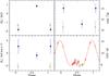 |
Fig. A.67 Mean longitudinal magnetic field (top left), crossover (bottom left), mean quadratic magnetic field (top right), and mean magnetic field modulus (bottom right) of the star HDE 335238, against rotation phase. The symbols are as described at the beginning of Appendix A. |
Appendix A.38: HDE 335238
In Paper I, we had argued that the rotation period of HDE 335238 must undoubtedly be between 40 and 50 days, but we had been unable to establish its value definitely, owing to the very unfortunate phase distribution of our observations. With all plausible values, the ⟨ B ⟩ data were concentrated in two narrow phase intervals, in which the mean field modulus measurements clustered around two values, 8.5 kG and 11.5 kG. We had ruled out the possibility that the higher of these two values, obtained in only 2 out of 16 observations, was spurious. Unfortunately, the 2 new ⟨ B ⟩ determinations reported here again happen to be close to 8.5 kG, so that they hardly add any new constraints on the shape of the variation curve. They do, however, enable us to rule out the preferred value of the rotation period tentatively proposed in Paper I, Prot = (44.0 ± 0.3) d. Instead, they favour a revised value Prot = (48.7 ± 0.1) d, which also seems consistent with Hipparcos photometric measurements of the star. This value is used to compute the phases against which the magnetic field data are plotted in Fig. A.67. From its consideration, it appears likely that the ⟨ B ⟩ curves shows a broad, fairly flat minimum and a sharper-peaked maximum, as in a number of other stars considered in this study. The uncertainty of the rotation period, and the very incomplete phase coverage of the observations, do not allow the ratio between the extrema of the field modulus to be exactly determined. But it cannot be smaller than 1.35. This provides an additional indication that the field structure in HDE 335238 must show some significant departure from a centred dipole.
Magnetic field determinations based on two new spectropolarimetric observations are also presented here. The field moments are diagnosed from lines of Fe ii and of Cr ii. With only three CASPEC spectra available (the two considered here, and one from Mathys & Hubrig 1997), we cannot definitely characterise the possible variability of those lines. Blending and, to some extent, systematic instrument-to-instrument differences, do not allow us to constrain this variability from consideration of our high-resolution spectra in natural light either.
With only 3 ⟨ Bz ⟩ measurements available, the variations of this field moment are not fully defined. But it definitely reverses its sign (hence if the field bears any resemblance to a dipole, both poles come into view as the star rotates). If the value of the rotation period proposed above is correct, the negative extremum of the longitudinal field may coincide roughly with the maximum of the field modulus, and conversely, the ⟨ Bz ⟩ positive extremum may occur during the broad minimum of ⟨ B ⟩, or possibly close to its little pronounced secondary maximum. The two new measurements of the quadratic field presented here are consistent with the field modulus variation, with the point close to phase 0 about 3 kG higher than the one close to phase 0.5. This difference is actually clearly seen in a visual comparison of the 2 CASPEC spectra with all the lines appearing much broader in the former than in the latter. In this picture, the ⟨ Bq ⟩ determination of Mathys & Hubrig (1997) is discrepant; this can almost certainly be assigned to its comparatively low quality, which was already mentioned for several other stars. This interpretation also applies to the discrepant crossover measurement of Mathys & Hubrig; the possible detection reported in that paper is almost certainly spurious. There is no definite evidence of radial velocity variations in our observations of HDE 335238.
Appendix A.39: HD 200311
The seven new determinations of the mean magnetic field modulus of HD 200311 unfortunately do not fill the gap of about one-third of the rotation cycle that was left in the phase coverage achieved in Paper I. This gap is clearly seen between phases 0.58 and 0.93 in Fig. A.68, in which the phases were computed using the value of the rotation period derived by Wade et al. (1997),  . The best-fit curve to our ⟨ B ⟩ data suggests the existence of a secondary maximum around phase 0.6. However, owing to the above-mentioned phase gap, this curve is not strongly constrained. Its marginal anarhmonicity (the M2 coefficient of the fit is determined at the 2.3σ level) is probably real but its apparent asymmetry seems difficult to reconcile with the almost perfect double-wave variation observed in photometry (Wade et al. 1997). The ratio between the extrema of ⟨ B ⟩ is not well defined either, but it cannot be signficantly smaller than 1.2, hence it is close to the upper limit for a centred dipole.
The northern declination of the star did not allow us to observe it with CASPEC. But ⟨ Bz ⟩ measurements have been published by Wade et al. (1997) and Leone et al. (2000). The longitudinal field reverses its sign as the star rotates, and to the achieved precision, its variation is sinusoidal. The phase relation between its extrema and those of the field modulus is not accurately defined owing to the pretty large uncertainties affecting the ⟨ Bz ⟩ determinations and to the gap in the ⟨ B ⟩ phase coverage, but in first approximation, the positive extremum of ⟨ Bz ⟩ seems to occur close to the phase of maximum of ⟨ B ⟩.
Consideration of Fig. A.69 suggests that the radial velocity of HD 200311 has been varying monotonically over the time interval covered by our observations. The standard deviation of our measurements about a straight-line fit, 1.1 km s-1, is consistent with their uncertainty. While a linear variation has no physical meaning, it may plausibly approximate well the actual shape of a fraction of the radial velocity curve of a spectroscopic binary with an orbital period much longer than the time separating our first and last observations (more than five years). A shorter period, of the order of 320 days, cannot be definitely ruled out, but this is most likely coincidental.
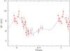 |
Fig. A.68 Mean magnetic field modulus of the star HD 200311, against rotation phase. The symbols are as described at the beginning of Appendix A. |
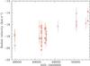 |
Fig. A.69 Radial velocity of HD 200311, against heliocentric Julian date. The symbols are as described at the beginning of Appendix A. |
Appendix A.40: HD 201601
HD 201601 is the prototype of the Ap stars with extremely long rotation periods. Its mean longitudinal magnetic field had been monotonically decreasing since the time of the measurements by Babcock (1958), about 60 yr ago (which may have been close to the positive extremum), until the latest determinations of Mathys & Hubrig (1997), in 1993 (see e.g. Fig. 37 of Mathys 1991). These authors reported a hint of flattening of the ⟨ Bz ⟩ curve, which raised suspicion that the star was approaching the phase of negative extremum of this field moment. Similarly, but on a shorter time span, the mean magnetic field modulus had been monotonically increasing from the time of its first measurement in 1988 (Mathys 1990) to the latest determination of Paper I, in 1995. We had suggested at the time that the phase of ⟨ B ⟩ maximum might be near.
Both suspicions are fully borne out by the six new ⟨ Bz ⟩ determinations and the seven new ⟨ B ⟩ measurements presented here. These show a slight, but definite, increase of the longitudinal field, as well as more pronounced progressive flattening of the field modulus variation curve (see Fig. A.70).
The negative extremum of ⟨ Bz ⟩ must have taken place very close to the time of the observations of Mathys & Hubrig (1997). The passage of the longitudinal field through that extremum is fully confirmed by more recent measurements of Bychkov et al. (2006), Savanov et al. (2014), and Bychkov et al. (2016).
The rotation period of HD 201601 must be considerably longer than the 67 yr time interval separating the earliest ⟨ Bz ⟩ measurement by Babcock (1958) from the latest measurement from Bychkov et al. (2016). The once preferred value of 77 yr (Leroy et al. 1994) now appears to be a very conservative lower limit. The value of 97.16 yr recently proposed by Bychkov et al. (2016) may be more realistic, but it must still be regarded with caution as it is the result of an extrapolation based on the assumption that the longitudinal field variation curve does not significantly depart from a sinusoid. That this cannot be taken for granted is illustrated by the anharmonicity of the ⟨ Bz ⟩ variations found for various other stars discussed in this paper. It may well be that the rotation period of HD 201601 is actually even longer than suggested by Bychkov et al. (2016).
On the other hand, the view that the mean magnetic field modulus was close to its maximum at the time of the new observations discussed here (1996–1998) is supported by the more recent determination of Savanov et al. (2006), on JD 2 452 920.6, which is achieved by application of the measurement technique and with one of the instrumental configurations used in the present paper. Accordingly, the fact that the derived value of ⟨ B ⟩ = (3879 ± 25) G is about 200 G smaller than our most recent values is a highly significant indication that the field modulus is decreasing, after passing through its maximum. Thus the phases of extremum of ⟨ B ⟩ and ⟨ Bz ⟩ appear to be in rough coincidence, which is not unusual; whether there is some small phase shift between them will have to be established by additional future measurements.
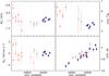 |
Fig. A.70 Mean longitudinal magnetic field (top left), crossover (bottom left), mean quadratic magnetic field (top right), and mean magnetic field modulus (bottom right) of the star HD 201601, against heliocentric Julian date. The symbols are as described at the beginning of Appendix A. |
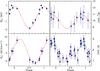 |
Fig. A.71 Mean longitudinal magnetic field (top left), crossover (bottom left), mean quadratic magnetic field (top right), and mean magnetic field modulus (bottom right) of the star HD 208217, against rotation phase. The symbols are as described at the beginning of Appendix A. |
The present determinations of the quadratic field of HD 201601 have on average smaller uncertainties than for any other star considered here. This must be related to the fact that the number of diagnostic lines analysed in this star is greater than in any other, which is consistent with the conclusion drawn by Mathys & Hubrig (2006) that the achievable uncertainty in quadratic field determinations scales like the inverse of the square root of the number of analysed lines. The apparent decrease of ⟨ Bq ⟩ seen in Fig. A.70 is more likely to reflect primarily the lower quality of the measurements of Mathys (1995b) and Mathys & Hubrig (1997) than to be real. If we compare the quadratic field values of 1996–1998 with contemporaneous field modulus data, the ratio between the two moments appears to be of the order of 1.15, showing reasonable mutual consistency.
The measurements of the crossover in HD 201601 presented here also have smaller errors than those of all other stars of the studied sample. Thus the fact that no crossover is detected is highly significant, and fully in line with the very long rotation period of the star.
Our observations cover too small a fraction of the rotation cycle of HD 201601 to assess the presence of variations of intensity of the Fe i and Fe ii lines analysed in the CASPEC spectra reliably. On the other hand, the absence of variations of the radial velocity of the star is convincingly established by the fact that the standard deviation of the values determined from the high-resolution spectra in natural light is a mere 0.3 km s-1. Our measurements are also very consistent with those of Carrier et al. (2002) with which they are mostly contemporaneous. Both data sets are also contemporaneous with the radial velocity determinations of Hildebrandt et al. (2000), indicating without ambiguity that the discrepant values reported by these authors must be spurious. However, HD 201601 is a visual binary, for which Stelzer et al. (2011) recently determined a preliminary orbital solution. The long orbital period that they derived, 274.5 yr, is compatible with the lack of significant radial velocity variations over the time interval covered by our data and those of Carrier et al. (2002).
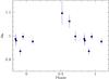 |
Fig. A.72 Variation with time of the average |
Appendix A.41: HD 208217
The seven new measurements of the mean longitudinal field magnetic field of HD 208217 presented here combine well with the data of Paper I using the value of the rotation period derived by Manfroid & Mathys (1997),  (Fig. A.71). They improve the definition of the shape of the ⟨ B ⟩ variation curve, which is significantly anharmonic, but with a secondary maximum that is considerably lower than the primary maximum, so that contrary to our speculation of Paper I, the field structure is different from a centred dipole. The ratio between the highest and lowest ⟨ B ⟩ values is fairly large, 1.27.
By contrast, the variations of the other field moments, determined through analysis of Fe ii lines in eight CASPEC spectra, do not significantly depart from sinusoids. The mean longitudinal magnetic field, which is measured here for the first time, reverses its sign as the star rotates, showing that both poles alternatively come into view. The phase coverage of the observations is unfortunate, as all concentrate in a little more than half a cycle. But within the limits of the achieved precision in its determination, the phase of maximum of ⟨ Bz ⟩ roughly coincides with that or the primary ⟨ B ⟩ maximum.
The difference between the phases of ⟨ Bz ⟩ positive extremum and of ⟨ Bq ⟩ maximum is somewhat below the formal significance threshold (see Tables 9 and 11); as a matter of fact, the phases of the extrema of the quadratic field variation curve are rather poorly constrained. The ratio between the quadratic field and the field modulus varies slightly with rotation phase around a value of about 1.25.
Crossover is definitely detected, not surprisingly since the v sini estimate that is obtained as a by-product of the quadratic field determination, 15 ± 5 km s-1, is significant. The rotational Doppler effect also shows in the distortion of the split components of the line Fe iiλ 6149.2, which as pointed out in Paper I complicates the determination of ⟨ B ⟩. The crossover variations lag in phase behind those of the longitudinal field by an amount that is not significantly different from a quarter of the rotation period, and its average over the rotation period is zero within the achieved accuracy; this behaviour is fully consistent with that generally observed (and expected) for this field moment (Mathys 1995a).
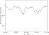 |
Fig. A.73 Portion of the spectrum of HD 213637 recorded on HJD 2451085.613, showing the lines Fe ii λ 6147.7 and Fe ii λ 6149.2. The blue wing of the latter is heavily blended by a line from an unidentified rare earth. The Cr ii λ 6147.1 line is not observed in this star at the considered epoch. |
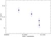 |
Fig. A.74 Mean magnetic field modulus of the star HD 213637, against heliocentric Julian date. |
The equivalent widths of the Fe ii lines used to diagnose the field moments discussed in the previous paragraph show some variability with rotation phase. As can be seen in Fig. A.72, they are stronger close to the positive extremum of ⟨ Bz ⟩ and weaker close to its negative extremum, suggesting a concentration of iron around the positive magnetic pole. Accordingly, the measured magnetic field values represent a convolution of the actual structure of the field with the inhomogeneous distribution of Fe over the stellar surface.
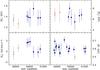 |
Fig. A.75 Mean longitudinal magnetic field (top left), crossover (bottom left), mean quadratic magnetic field (top right), and mean magnetic field modulus (bottom right) of the star HD 216018, against heliocentric Julian date. The symbols are as described at the beginning of Appendix A. |
As already reported in Paper I, the radial velocity of HD 208217 is variable. Our attempts to determine an orbital period were unsuccessful owing to very strong aliasing. The difficulty is almost certainly further compounded by the rather large uncertainty affecting the radial velocity determinations in our high-resolution spectra, owing to the strong blend affecting the blue component of the line Fe iiλ 6149.2 and to its distortion by the combination of the Zeeman effect at different locations on the stellar surface with rotational Doppler effect. The latter furthermore contributes to some extent to the radial velocity variations. However, the rotation period does not clearly appear in a frequency analysis of the radial velocity measurements. In any case, the amplitude of the variations (more than 20 km s-1 peak-to-peak) is sufficient so that there is no question that they are real and that they cannot be fully accounted for by rotation, hence that the star must be a spectroscopic binary. It is actually an astrometric binary (Makarov & Kaplan 2005); it is impossible to determine at this stage if the astrometric companion is the same as the spectroscopic one, or if HD 208217 is part of a multiple system.
Appendix A.42: HD 213637
Resolved magnetically split lines were discovered in the little known roAp star HD 213637 (Martinez et al. 1997) on our high-resolution spectrum obtained on November 11, 1997. We announced this finding in an oral presentation at the conference on “Magnetic fields across the Hertzsprung-Russell diagram” held in Santiago in January 2001 (Mathys 2001). Seven ⟨ B ⟩ measurements were reported at the conference on “Magnetic fields in O, B, and A stars” held in Mmabatho in November 2002 (Mathys 2003). An independent discovery report, based on a spectrum taken on April 17, 2002, was published by Kochukhov (2003). This observation is posterior to all measurements presented here.
The resolution of the Fe ii λ 6149.2 line is illustrated in the portion of one of our high-resolution spectra that is shown in Fig. A.73. The four determinations of the mean magnetic field modulus that we obtained are consistent with a monotonic decrease over the 115 day time interval that they span (see Fig. A.74), but they do not rule out a shorter rotation period. The distortion of the lines appearing in Fig. A.73 may plausibly be caused by the rotational Doppler effect. On the other hand, the value ⟨ B ⟩ = (5.5 ± 0.1) kG measured by Kochukhov (2003) indicates that the star has passed through at least one, and possibly several minima of its field modulus between 1998 and 2002.
To estimate the uncertainties affecting our determinations of the mean magnetic field modulus of this star, we computed their standard deviation about a least-squares fit by a straight line, obtaining a value of 40 G. Admittedly, this is meaningful only if the rotation period is longer than the time interval over which those data have been obtained, so that the estimated error must be regarded with caution.
All our CASPEC observing nights took place before the discovery of magnetically resolved lines in HD 213637. By chance, a single spectropolarimetric observation of it had been obtained prior to this discovery. Based on it, we report the measurement of a longitudinal field slightly above the threshold of formal significance, at the 3.6σ level. We also determined a value of the quadratic field. The latter cannot be directly compared to the field modulus data, since the measurements of the two field moments were obtained at different epochs, at unknown but presumably different rotation phases; but the orders of magnitude are not incompatible. In contrast, the value of ⟨ Bz ⟩ = (230 ± 63) G obtained here is significantly different from the one published by Hubrig et al. (2004b), 740 ± 50 G, from low-resolution spectropolarimetric observations performed with FORS-1 at the VLT. Even allowing for possible discrepancies resulting from the usage of different field determination techniques, the difference between the two measurements most likely reflects actual variations of ⟨ Bz ⟩ (not surprisingly, considering the variability of ⟨ B ⟩). No crossover was detected, which tends to favour a long period.
Appendix A.43: HD 216018
Our suspicion in Paper I that the mean magnetic field modulus was starting to increase towards the end of our series of observations, after remaining constant for about two years, is not supported by the five new ⟨ B ⟩ measurements presented here. Actually, it was found that the last three ⟨ B ⟩ determinations of Paper I were incorrect. The reason is not definitely established, although it can be speculated that the strong blend affecting the blue component of the line Fe iiλ 6149.2 had not been properly dealt with. Those three measurements have been redone, and their outcome appears in Table 5 and in Fig. A.75. Following that revision, it appears that the field modulus of HD 216018 has shown no significant variation over the time interval covered by our entire data set, which is slightly longer than six years. The standard deviation of all our measurements, 47 G, is compatible with a constant field over the considered period, if one takes into account the difficulty to measure the heavily blended blue component of Fe iiλ 6149.2 with ultimate precision.
The spectrum of HD 216018 is extremely dense, so that it was impossible to find enough lines of a single ion, or even of a single chemical element, that were sufficiently free from blends to be used for magnetic field diagnosis. Like the mean field modulus, the longitudinal field and the quadratic field, which were determined from the analysis of a sample of lines of Fe i, Fe ii, and Cr ii, do not show any variability over the time span of more than five years covered by our measurements and the earlier measurements of Mathys & Hubrig (1997). The ratio between the quadratic field and the field modulus is close to 1.2. No crossover is detected.
The data described above indicate either that HD 216018 is not variable (possibly seen rotation-pole on) or that its rotation period is much longer than six years.
The standard deviation of all the radial velocity measurements based on our high-resolution spectra recorded in natural light is only 0.3 km s-1: we do not detect any significant variability. As for the field modulus, the claim in Paper I that the measurements of the last observing season under consideration were starting to show a slow decrease of the radial velocity was the result of incorrect determinations.
Appendix B: Revised mean quadratic magnetic field determinations
Revised mean quadratic magnetic field measurements.
In this Appendix, we present the revised values of the mean quadratic magnetic field that we derived as described in Sect. 3.2 for the stars studied by Mathys (1995b). Namely, for each of those stars that had been observed at least at three different epochs, we computed for each diagnostic line the average of the values of measured for this line by Mathys (1995b) at the various epochs. We used those averages to determine the parameters a1 and a3 of Eq. (9), then computed by application of Eq. (12), and finally derived ⟨ Bq ⟩ at each epoch by application of Eq. (13).
The updated values of ⟨ Bq ⟩ that were obtained in that way are presented in Table B.1, both for the stars with resolved magnetically split lines that were included in the sample of Mathys (1995b) and for the other stars of that study for which improved values of the quadratic field could be obtained (n is the number of diagnostic lines from which the corresponding value of ⟨ Bq ⟩ was determined). These values supersede those published by Mathys (1995b).
Two of the stars for which Mathys (1995b) had obtained observations at a sufficient number of epochs for application of the above-described revised analysis procedure, HD 74521 and HD 175362, were omitted from Table B.1. The quadratic field of the former is below the detection limit, similar to HD 188041 in this paper (see Appendix A.36); the apparently significant values derived by Mathys (1995b) most likely were overestimates. The same limitation affects the determination of the quadratic field of HD 153882 for the two observations obtained on JD 2 446 896. For HD 175362, the assumption that the fit parameters a1 and a3 have the same values at all epochs of observation, which underlies the method applied for determination of the revised values of ⟨ Bq ⟩, appears to break down, possibly because the diagnostic lines that are used pertain to different elements and ions, and/or because the distribution of those elements over the stellar surface is very inhomogeneous (see Table 3 and Figs. 26 to 31 of Mathys 1991).
Appendix C: Pulsational crossover
In Sect. 5.3, we introduced the pulsational crossover mechanism as a possible interpretation of results of our crossover measurements that cannot be explained by the classical rotational crossover mechanism. The occurrence of pulsational crossover has been related to the large variation of the radial velocity pulsation amplitude with photospheric depth in roAp stars. The latter implies that there are significant velocity gradients in the line-forming region. In this Appendix, we show how the existence of such gradients along the line of sight in the region of formation of spectral lines that are used for determination of the magnetic field moments generates a non-zero crossover in these lines, that is, non-zero values of the second-order moments of their Stokes V profiles about their respective centres.
For the sake of simplicity, we assume that a single pulsation mode is excited and that the rotational velocity of the star is zero. These restrictions have no effect on the conclusions drawn here. We also assume that observations are obtained with an exposure time equal to one or several pulsation period(s) of the star, so that the observed spectrum is averaged over this pulsation period. This is appropriate since our purpose here is to demonstrate the existence of a net, non-zero effect that does not average out over a stellar pulsation period.
Then, the second-order moment of the Stokes V profile of a spectral line about the central wavelength λI of its observed Stokes I profile can be expressed as ![Mathematical equation: \appendix \setcounter{section}{3} \begin{eqnarray} &&\R{2}{V}={\cal N}\,\intxy\int_0^{2\pi}{\rm d}\psi\nonumber\\ &&\times\int V[x,y,\psi;\llo-\dlp;\Hvec(x,y)]\,(\llo)^2\,{\rm d}\lambda,\nonumber\\ \label{eq:R2Va} \end{eqnarray}](/articles/aa/full_html/2017/05/aa28429-16/aa28429-16-eq839.png) (C.1)where (x,y) are the coordinates of a point on the stellar disk, in units of the stellar radius; B(x,y) is the local magnetic vector at that point; Δλp(x,y;ψ) is the wavelength shift of the centre of the emergent line in Stokes I at that point caused by pulsation at pulsation phase ψ, and
(C.1)where (x,y) are the coordinates of a point on the stellar disk, in units of the stellar radius; B(x,y) is the local magnetic vector at that point; Δλp(x,y;ψ) is the wavelength shift of the centre of the emergent line in Stokes I at that point caused by pulsation at pulsation phase ψ, and  is a normalisation constant. The λ integration extends over the whole width of the line (for details, see Mathys 1988). The shape of the local emergent V profile includes its distortion by the pulsation, which varies across the stellar surface and with pulsation phase. The velocity gradients that are present in the line-forming region, as a result of the dependence of the pulsation amplitude on optical depth, create departures from anti-symmetry in this profile (Landi Degl’Innocenti & Landolfi 1983).
Performing the change of variable λ → λ + Δλp(x,y;ψ), Eq. (C.1) can be rewritten as ![Mathematical equation: \appendix \setcounter{section}{3} \begin{equation} \R{2}{V}={\cal N}\left[I_0(\lambda_I)+2\,I_1(\lambda_I)+I_2(\lambda_I)\right], \label{eq:R2Vb} \end{equation}](/articles/aa/full_html/2017/05/aa28429-16/aa28429-16-eq846.png) (C.2)with
(C.2)with ![Mathematical equation: \appendix \setcounter{section}{3} \begin{eqnarray} I_0(\lambda_I)&=&\intxy\,\int_0^{2\pi}{\rm d}\psi\nonumber\\ &&\times\int V[x,y,\psi;\llo;\Hvec(x,y)]\,(\llo)^2\,{\rm d}\lambda, \label{eq:I0}\\ I_1(\lambda_I)&=&\intxy\,\int_0^{2\pi}\dlp\,{\rm d}\psi\nonumber\\ &&\times\int V[x,y,\psi;\llo;\Hvec(x,y)]\,(\llo)\,{\rm d}\lambda, \label{eq:I1}\\ I_2(\lambda_I)&=&\intxy\,\int_0^{2\pi}\Delta\lambda^2_{\rm p}(x,y;\psi) \,{\rm d}\psi\nonumber\\ &&\times\int V[x,y,\psi;\llo;\Hvec(x,y)]\,{\rm d}\lambda. \label{eq:I2} \end{eqnarray}](/articles/aa/full_html/2017/05/aa28429-16/aa28429-16-eq847.png)
The non-antisymmetric emergent Stokes V profiles can always be expressed as the sum of a symmetric part and of an antisymmetric part as follows: ![Mathematical equation: \appendix \setcounter{section}{3} \begin{eqnarray} V[x,y,\psi;\llo;\Hvec(x,y)]&=&V_{\rm S}[x,y,\psi;\llo;\Hvec(x,y)]\nonumber\\ &&+V_{\rm A}[x,y,\psi;\llo;\Hvec(x,y)],\nonumber\\ \end{eqnarray}](/articles/aa/full_html/2017/05/aa28429-16/aa28429-16-eq848.png) (C.6)with
(C.6)with ![Mathematical equation: \appendix \setcounter{section}{3} \begin{eqnarray} V_{\rm S}[x,y,\psi;\llo;\Hvec(x,y)]&=&V_{\rm S}[x,y,\psi;\lambda_I-\lambda;\Hvec(x,y)], \\ V_{\rm A}[x,y,\psi;\llo;\Hvec(x,y)]&=&-V_{\rm A}[x,y,\psi;\lambda_I-\lambda;\Hvec(x,y)]. \end{eqnarray}](/articles/aa/full_html/2017/05/aa28429-16/aa28429-16-eq849.png) Because of the integration over the wavelengths, only the symmetric part of the Stokes V profile can make a non-zero contribution to I0(λI) and I2(λI). Conversely, this part cancels out in the wavelength integration of I1(λI).
Because of the integration over the wavelengths, only the symmetric part of the Stokes V profile can make a non-zero contribution to I0(λI) and I2(λI). Conversely, this part cancels out in the wavelength integration of I1(λI).
Pulsation phases separated by π radians are characterised by opposite velocity fields, so that  (C.9)In the absence of velocity gradients, the Stokes V profile is anti-symmetric: the anti-symmetric part, VA, must be independent of the pulsation phase. Therefore the term containing this part cancels out in the integration on ψ in I1(λI), so that I1(λI) = 0.
Thus only the symmetric part of the local Stokes V profiles can make non-zero contributions to the observable crossover via the terms I0(λI) and I2(λI) of Eq. (C.2). Accordingly Eq. (C.1) reduces to ![Mathematical equation: \appendix \setcounter{section}{3} \begin{eqnarray} \R{2}{V}&=&{\cal N}\,\intxy\,\int_0^{2\pi}{\rm d}\psi\nonumber\\ &&\times\int V_{\rm S}[x,y,\psi;\llo;\Hvec(x,y)]\,(\llo)^2\,{\rm d}\lambda\nonumber\\ &&+{\cal N}\,\intxy\,\int_0^{2\pi}\Delta\lambda^2_{\rm p}(x,y;\psi)\,{\rm d}\psi\nonumber\\ &&\times\int V_{\rm S}[x,y,\psi;\llo;\Hvec(x,y)]\,{\rm d}\lambda. \end{eqnarray}](/articles/aa/full_html/2017/05/aa28429-16/aa28429-16-eq857.png) (C.10)The symmetric part of the local V profiles should not be expected to average out by integration over the pulsation phases, as long as the variation of the amplitude of pulsation across the photospheric layers is not very small compared to the thermal Doppler width of the lines (Landolfi & Landi Degl’Innocenti 1996). This condition is obviously fulfilled in at least a fraction of the known roAp stars, since we do actually observe a dependence in their pulsation amplitude on the line formation depth. Thus the effect described in this Appendix can indeed account, qualitatively, for the occurrence of crossover in pulsating Ap stars, even if these stars have negligible rotation.
(C.10)The symmetric part of the local V profiles should not be expected to average out by integration over the pulsation phases, as long as the variation of the amplitude of pulsation across the photospheric layers is not very small compared to the thermal Doppler width of the lines (Landolfi & Landi Degl’Innocenti 1996). This condition is obviously fulfilled in at least a fraction of the known roAp stars, since we do actually observe a dependence in their pulsation amplitude on the line formation depth. Thus the effect described in this Appendix can indeed account, qualitatively, for the occurrence of crossover in pulsating Ap stars, even if these stars have negligible rotation.
All Tables
Ap stars with resolved magnetically split lines: stars for which new measurements of the mean magnetic field modulus are presented in this paper.
Ap stars with resolved magnetically split lines: stars with magnetic measurements from the literature.
Observing runs and instrumental configurations: high-resolution spectra in natural light.
Variation of the mean longitudinal magnetic field: least-squares fit parameters for stars with ⟨ Bz ⟩ data in this paper.
New or revised orbital elements of spectroscopic binaries. The second row for each entry gives its standard deviation.
Magnetic parameters of Ap stars with resolved magnetically split lines: stars with ⟨ B ⟩ data from the literature.
Variation of the mean magnetic field modulus: least-squares fit parameters for data from the literature.
Variation of the mean longitudinal magnetic field: least-squares fit parameters for data from the literature.
Summary of crossover measurements in Ap stars with resolved magnetically split lines.
Ap stars with magnetically resolved lines with a known orbital period (or a meaningful lower limit thereof).
Ap stars with published reliable orbital and rotation periods, not known to show magnetically resolved lines.
All Figures
|
Fig. 1 Histogram showing the distribution of the phase-averaged mean magnetic field moduli of the 84 Ap stars with resolved magnetically split lines presently known. The shaded part of the histogram corresponds to those stars whose field modulus has been measured throughout their rotation cycle (see text). |
| In the text | |
|
Fig. 2 Observed average of the mean magnetic field modulus against rotation period. Dots: stars with known rotation periods; triangles: stars for which only the lower limit of the period is known. Open symbols are used to distinguish those stars for which existing measurements do not cover the whole rotation cycle. The horizontal and vertical dashed lines, corresponding to ⟨ B ⟩ av = 7.5 kG and Prot = 150 d, respectively, emphasise the absence of very strong magnetic fields in the stars with the slowest rotation (see text for details). |
| In the text | |
|
Fig. 3 Distribution of the ratio q between the observed extrema of mean magnetic field moduli of the 66 Ap stars with resolved magnetically split lines presently known for which more than one measurement of ⟨ B ⟩ is available. Although HD 96237 was observed twice by Freyhammer et al. (2008), its spectral lines were not resolved in the first epoch spectrum. The shaded part of the histogram corresponds to those stars that have been observed throughout their rotation cycle (see text). |
| In the text | |
|
Fig. 4 Ratio q of the observed extrema of the mean magnetic field modulus against rotation period. Dots: stars with known rotation periods; triangles: stars for which only the lower limit of the period is known. Open symbols are used to distinguish those stars for which existing measurements do not cover the whole rotation cycle. The horizontal and vertical dashed (red) lines, corresponding to q = 1.3 and Prot = 100 d, respectively, emphasise the tendency for higher values of q to have a higher rate of occurrence in the stars with the slowest rotation. The horizontal dotted (blue) line corresponds to the upper limit of q for a centred dipole (see text). |
| In the text | |
|
Fig. 5 Ratio M2/M1 of the fit coefficients given in Tables 8 and 15 against rotation period. Open circles: stars showing ⟨ Bz ⟩ reversal; dots: stars in which ⟨ Bz ⟩ has a constant sign; open triangle: star for which no ⟨ Bz ⟩ measurements exist. For a fraction of the stars, the error bar is shorter than the size of the representative symbol. The horizontal (solid) line corresponds to the stars for which the curve of variation of ⟨ Bz ⟩ does not significantly depart from a sinusoid (M2 = 0). The two vertical (dashed) lines emphasise the tendency for anharmonicity of the mean field modulus variations to be restricted to rotation periods shorter than Prot = 100 d or greater than Prot = 1000 d. |
| In the text | |
|
Fig. 6 Difference between the primary and secondary maxima of the mean magnetic field modulus against the difference between its two minima; both differences are normalised via division by the difference between the primary maximum and primary minimum. Open circles represent stars whose longitudinal field reverses its sign over a rotation period; the dot corresponds to a star with non-reversing longitudinal field. The dashed line is drawn to help the eye visualise the fact that the difference between the minima is generally smaller, and never much greater than the difference between the maxima. The only star above this line is HD 200311, for which no ⟨ B ⟩ data could be obtained between phases 0.6 and 0.9. More observations of the star in this phase range might possibly shift its representative point below the dashed line. |
| In the text | |
|
Fig. 7 Histogram showing the distribution of the root-mean-square longitudinal magnetic field of the 49 Ap stars with resolved magnetically split lines for which this field moment was measured at least once. The shaded part of the histogram corresponds to those stars whose longitudinal field has been measured throughout their rotation cycle (see text). |
| In the text | |
|
Fig. 8 Observed root-mean-square longitudinal field against the observed average of the mean magnetic field modulus. Open symbols are used to distinguish those stars for which either or both of ⟨ Bz ⟩ rms and ⟨ B ⟩ av were computed using less than 7 individual measurements of, resp., ⟨ Bz ⟩ and ⟨ B ⟩; triangles are used for field modulus values from the literature. The dashed line corresponds to ⟨ Bz ⟩ rms = ⟨ B ⟩ av/ 3. For only two stars (identified in the figure), the representative points are clearly above this line. However this is significant only for HD 215441, since the number of measurements of HD 157751 is insufficient (see text). The dotted vertical line corresponds to ⟨ B ⟩ av = 2.8 kG; it emphasises the discontinuity at the low end of the distribution of ⟨ B ⟩ av, discussed in Sect. 5.1. |
| In the text | |
|
Fig. 9 Relative amplitude q of the variation of the mean magnetic field modulus against the ratio r of the extrema of the mean longitudinal field (see text). Dots identify values of q computed from the ⟨ B ⟩ data of this paper and of Paper I; triangles are used for field moduli from the literature. Filled symbols correspond to stars for which the ⟨ Bz ⟩ measurements are based on CASPEC observations (this paper; Mathys 1994; Mathys & Hubrig 1997), open symbols to other good ⟨ Bz ⟩ measurements from the literature (references given in the text). The dashed diagonal line, q = (3−r)/2, emphasises the concentration of the majority of the stars of the sample in the lower left part of the figure: namely, high amplitudes of variation of ⟨ B ⟩ are observed when both the positive and negative magnetic poles of the star come into sight during its rotation cycle. |
| In the text | |
|
Fig. 10 Ratio r of the extrema of the mean longitudinal magnetic field (see text) against rotation period. Dots: stars with known rotation periods; triangles: stars for which only the lower limit of the period is known. Open symbols are used to distinguish those stars for which existing measurements do not cover the whole rotation cycle. Stars with representative points below the long-dashed horizontal line have reversing mean longitudinal fields. The two vertical (dashed) lines emphasise the tendency for longitudinal fields showing sign reversals to be restricted to rotation periods shorter than Prot = 100 d or longer than Prot = 1000 d. |
| In the text | |
|
Fig. 11 Phase difference φZ1−φM1 (modulo 1) between the fundamentals of the fits of the measurements of ⟨ Bz ⟩ and ⟨ B ⟩ by functions of the forms given in Eqs. (16) or (17), against stellar rotation period. Open symbols: stars showing ⟨ Bz ⟩ reversal; filled symbols: stars in which ⟨ Bz ⟩ has a constant sign. Among the latter, stars with positive values of ⟨ Bz ⟩ are represented by dots, while triangles correspond to negative values of ⟨ Bz ⟩. For a fraction of the stars, the error bar is shorter than the size of the representative symbol. Shaded zones correspond to forbidden regions where representative points of stars with dipole-like fields are not expected to be found. We identified three stars that depart from this expected behaviour. |
| In the text | |
|
Fig. 12 Observed average of the mean quadratic magnetic field against the observed average of the mean magnetic field modulus. Open symbols are used to distinguish those stars for which either or both of ⟨ Bq ⟩ av and ⟨ B ⟩ av were computed using less than 7 individual measurements of ⟨ Bq ⟩ and ⟨ B ⟩, respectively. The short-dashed line corresponds to ⟨ Bq ⟩ av = ⟨ B ⟩ av. The long-dashed line represents the least-squares fit of the observed relation between ⟨ Bq ⟩ av and ⟨ B ⟩ av; it is based only on the stars for which at least 7 measurements of both ⟨ Bq ⟩ and ⟨ B ⟩ are available. |
| In the text | |
|
Fig. 13 Relative amplitude p of the mean quadratic magnetic field variations against that of the mean magnetic field modulus variations (q). Open symbols: stars showing ⟨ Bz ⟩ reversal; filled symbols: stars in which ⟨ Bz ⟩ has a constant sign. Among the latter, triangles are used to distinguish those stars in which the phase of maximum ⟨ B ⟩ coincides approximately with the phase of lowest absolute value of ⟨ Bz ⟩, while dots are used when ⟨ B ⟩ maximum occurs close to the phase of highest absolute value of ⟨ Bz ⟩. |
| In the text | |
|
Fig. 14 Phase difference φQ1−φM1 between the fundamenals of the fits of the measurements of ⟨ Bq ⟩ and ⟨ B ⟩ by functions of the forms given in Eqs. (16) and (17), against stellar rotation period. The meaning of the symbols is the same as in Fig. 13. Shaded zones correspond to forbidden regions where points are not expected to be found (see text for details). Two stars that depart from this expected behaviour (one of them marginally) are identified. |
| In the text | |
|
Fig. 15 Histogram showing the distribution of the rotation periods of the 50 Ap stars with resolved magnetically split lines for which their value has been determined (shaded part of the histogram) or for which a meaningfully lower limit has been obtained (see text). |
| In the text | |
|
Fig. 16 Rotation period is plotted against the orbital period for the spectroscopic binaries for which these two periods are sufficiently constrained by the existing observations. Asterisks and crosses represent stars not known to have magnetically resolved lines, for which both periods were retrieved from the literature; crosses distinguish those for which uncertainties remain about some of the relevant parameters (see text). All other symbols correspond to Ap stars with magnetically resolved lines studied in detail in this paper. Dots identify those stars for which both periods are exactly known; open circles, stars with fully determined rotation periods for which only a lower limit of the orbital period has been obtained so far; filled triangles, stars with a known orbital period but only a lower limit of the rotation period; and open triangles, stars that have only been observed over a fraction of both their rotation and orbital periods. The short-dashed diagonal line represents the locus log Prot = 3.9−log Porb. The long-dashed horizontal line corresponds to Prot = 50 d and the long-dashed vertical line to Porb = 1000 d. |
| In the text | |
|
Fig. 17 Comparison between the distribution of the orbital periods of binaries containing an Ap star with a rotation period shorter (solid blue line) and greater (dashed red line) than 50 days. |
| In the text | |
|
Fig. A.1 Mean longitudinal magnetic field (top left), crossover (bottom left), mean quadratic magnetic field (top right), and mean magnetic field modulus (bottom right) of the star HD 965, against heliocentric Julian date. The symbols are as described at the beginning of Appendix A. |
| In the text | |
|
Fig. A.2 Mean longitudinal magnetic field (top left), crossover (bottom left), mean quadratic magnetic field (top right), and mean magnetic field modulus (bottom right) of the star HD 2453, against rotation phase. For the longitudinal field, measurements of Babcock (1958; open triangles) and Wolff (1975; crosses) are also shown. The other symbols are as described at the beginning of Appendix A. |
| In the text | |
|
Fig. A.3 Our radial velocity measurements for HD 2453 are plotted together with those of Carrier et al. (2002) against heliocentric Julian date. Dots correspond to the Carrier et al. data; all other symbols refer to our high-resolution spectra obtained with various instrumental configurations, as indicated in Table 3. |
| In the text | |
|
Fig. A.4 Mean magnetic field modulus of the star HD 9996, against rotation phase. The symbols are as described at the beginning of Appendix A. |
| In the text | |
|
Fig. A.5 Portion of the spectrum of HD 9996 recorded at two different epochs (resp. rotation phases), identified above (resp. below) each tracing (the epochs are given as HJD−2 400 000), showing the lines Cr ii λ 6147.1, Fe ii λ 6147.7, and Fe ii λ 6149.2. At the second epoch, the blue wing of the latter is blended with an unidentified rare earth line. That spectrum is affected by a cosmic ray hit between the lines Cr ii λ 6147.1 and Fe ii λ 6147.7. |
| In the text | |
|
Fig. A.6 Upper panel: our radial velocity measurements for HD 9996 are plotted together with those of Carrier et al. (2002) against orbital phase. The solid curve corresponds to the orbital solution given in Table 12. The time T0 of periastron passage is adopted as phase origin. Bottom panel: plot of the differences O−C between the observed values of the radial velocity and the predicted values computed from the orbital solution. The dotted lines correspond to ± 1 rms deviation of the observational data about the orbital solution (dashed line). Dots represent the data from Carrier et al.; all other symbols refer to our high-resolution spectra obtained with various instrumental configurations, as indicated in Table 3. |
| In the text | |
|
Fig. A.7 Mean magnetic field modulus of the star HD 12288, against rotation phase. |
| In the text | |
|
Fig. A.8 Upper panel: our radial velocity measurements for HD 12288 are plotted together with those of Carrier et al. (2002) against orbital phase. The solid curve corresponds to the orbital solution given in Table 12. The time T0 of periastron passage is adopted as phase origin. Bottom panel: plot of the differences O−C between the observed values of the radial velocity and the predicted values computed from the orbital solution. The dotted lines correspond to ±1 rms deviation of the observational data about the orbital solution (dashed line). Dots represent the data from Carrier et al.; all other symbols refer to our high-resolution spectra obtained with various instrumental configurations, as indicated in Table 3. |
| In the text | |
|
Fig. A.9 Mean magnetic field modulus of the star HD 14437, against rotation phase. The symbols are as described at the beginning of Appendix A. |
| In the text | |
|
Fig. A.10 Mean magnetic field modulus of the star HD 18078, against rotation phase. The symbols are as described at the beginning of Appendix A. |
| In the text | |
|
Fig. A.11 Our radial velocity measurements for HD 18078 are plotted together with those of Carrier et al. (2002) against heliocentric Julian date. Dots correspond to the Carrier et al. data; all other symbols refer to our high-resolution spectra obtained with various instrumental configurations, as indicated in Table 3. |
| In the text | |
|
Fig. A.12 Mean longitudinal magnetic field (top left), crossover (bottom left), mean quadratic magnetic field (top right), and mean magnetic field modulus (bottom right) of the star HD 29578, against heliocentric Julian date. The symbols are as described at the beginning of Appendix A. |
| In the text | |
|
Fig. A.13 Upper panel: our radial velocity measurements for HD 29578 are plotted against orbital phase. The solid curve corresponds to the orbital solution given in Table 12. The time T0 of periastron passage is adopted as phase origin. Bottom panel: plot of the differences O−C between the observed values of the radial velocity and the predicted values computed from the orbital solution. The dotted lines correspond to ±1 rms deviation of the observational data about the orbital solution (dashed line). Open squares represent our CASPEC observations; all other symbols refer to our high-resolution spectra obtained with various instrumental configurations, as indicated in Table 3. |
| In the text | |
|
Fig. A.14 Portion of the spectrum of HD 47103 recorded on HJD 2 450 427.689, showing the lines Cr ii λ 6147.1 (affected by a cosmic ray hit), Fe ii λ 6147.7, and Fe ii λ 6149.2. |
| In the text | |
|
Fig. A.15 Mean longitudinal magnetic field (top left), crossover (bottom left), mean quadratic magnetic field (top right), and mean magnetic field modulus (bottom right) of the star HD 47103, against heliocentric Julian date. The symbols are as described at the beginning of Appendix A. |
| In the text | |
|
Fig. A.16 Mean longitudinal magnetic field (top left), crossover (bottom left), mean quadratic magnetic field (top right), and mean magnetic field modulus (bottom right) of the star HD 50169, against heliocentric Julian date. The symbols are as described at the beginning of Appendix A. |
| In the text | |
|
Fig. A.17 Mean longitudinal magnetic field of the star HD 50169, against heliocentric Julian date. Crosses represent the measurements of Babcock (1958), and the filled square is the point obtained by Romanyuk et al. (2014). The other symbols are as described at the beginning of Appendix A. |
| In the text | |
|
Fig. A.18 Upper panel: our radial velocity measurements for HD 50169 are plotted against orbital phase. The solid curve corresponds to the orbital solution given in Table 12. The time T0 of periastron passage is adopted as phase origin. Bottom panel: plot of the differences O−C between the observed values of the radial velocity and the predicted values computed from the orbital solution. The dotted lines correspond to ± 1 rms deviation of the observational data about the orbital solution (dashed line). Open triangles represent the data from Carrier et al. and asterisks our CASPEC observations; all other symbols refer to our high-resolution spectra obtained with various instrumental configurations, as indicated in Table 3. |
| In the text | |
|
Fig. A.19 Portion of the spectrum of HD 51684 recorded on HJD 2 450 427.623, showing the lines Cr ii λ 6147.1, Fe ii λ 6147.7, and Fe ii λ 6149.2. |
| In the text | |
|
Fig. A.20 Mean longitudinal magnetic field (top left), crossover (bottom left), mean quadratic magnetic field (top right), and mean magnetic field modulus (bottom right) of the star HD 51684, against rotation phase. The symbols are as described at the beginning of Appendix A. |
| In the text | |
|
Fig. A.21 Mean longitudinal magnetic field (top left), crossover (bottom left), mean quadratic magnetic field (top right), and mean magnetic field modulus (bottom right) of the star HD 55719, against heliocentric Julian date. The symbols are as described at the beginning of Appendix A. |
| In the text | |
|
Fig. A.22 Upper panel: our radial velocity measurements for HD 55719 are plotted together with those of Bonsack (1976) against orbital phase. The solid curve corresponds to the orbital solution given in Table 12. The time T0 of periastron passage is adopted as phase origin. Bottom panel: plot of the differences O−C between the observed values of the radial velocity and the predicted values computed from the orbital solution. The dotted lines correspond to ±1 rms deviation of the observational data about the orbital solution (dashed line). Open triangles represent the data from Bonsack and open squares our CASPEC observations; all other symbols refer to our high-resolution spectra obtained with various instrumental configurations, as indicated in Table 3. |
| In the text | |
|
Fig. A.23 Mean magnetic field modulus of the star HD 59435, against rotation phase. The symbols are as described at the beginning of Appendix A. |
| In the text | |
|
Fig. A.24 Mean longitudinal magnetic field (top left), crossover (bottom left), mean quadratic magnetic field (top right), and mean magnetic field modulus (bottom right) of the star HD 61468, against rotation phase. The symbols are as described at the beginning of Appendix A. |
| In the text | |
|
Fig. A.25 Upper panel: our radial velocity measurements for HD 61468 are plotted against orbital phase. The solid curve corresponds to the orbital solution given in Table 12. The time T0 of periastron passage is adopted as phase origin. Bottom panel: plot of the differences O−C between the observed values of the radial velocity and the predicted values computed from the orbital solution. The dotted lines correspond to ± 1 rms deviation of the observational data about the orbital solution (dashed line). Open squares represent our CASPEC observations; all other symbols refer to our high-resolution spectra obtained with various instrumental configurations, as indicated in Table 3. |
| In the text | |
|
Fig. A.26 Mean magnetic field modulus of the star HD 65339, against rotation phase. The symbols are as described at the beginning of Appendix A. |
| In the text | |
|
Fig. A.27 Mean longitudinal magnetic field (top left), crossover (bottom left), mean quadratic magnetic field (top right), and mean magnetic field modulus (bottom right) of the star HD 70331, against rotation phase, computed assuming that the rotation period is 1 |
| In the text | |
|
Fig. A.28 Mean longitudinal magnetic field (top left), crossover (bottom left), mean quadratic magnetic field (top right), and mean magnetic field modulus (bottom right) of the star HD 70331, against rotation phase, computed assuming that the rotation period is 1 |
| In the text | |
|
Fig. A.29 Mean longitudinal magnetic field (top left), crossover (bottom left), mean quadratic magnetic field (top right), and mean magnetic field modulus (bottom right) of the star HD 75445, against rotation phase. The symbols are as described at the beginning of Appendix A. |
| In the text | |
|
Fig. A.30 Mean longitudinal magnetic field (top left), crossover (bottom left), mean quadratic magnetic field (top right), and mean magnetic field modulus (bottom right) of the star HD 81009, against rotation phase. The symbols are as described at the beginning of Appendix A. |
| In the text | |
|
Fig. A.31 Variation with rotation phase of the average |
| In the text | |
|
Fig. A.32 Mean longitudinal magnetic field (top left), crossover (bottom left), mean quadratic magnetic field (top right), and mean magnetic field modulus (bottom right) of the star HD 93507, against rotation phase. The symbols are as described at the beginning of Appendix A. |
| In the text | |
|
Fig. A.33 Variation with rotation phase of the average |
| In the text | |
|
Fig. A.34 Mean longitudinal magnetic field (top left), crossover (bottom left), mean quadratic magnetic field (top right), and mean magnetic field modulus (bottom right) of the star HD 94660, against rotation phase. The symbols are as described at the beginning of Appendix A. |
| In the text | |
|
Fig. A.35 Upper panel: our radial velocity measurements for HD 94660 are plotted together with those of Bailey et al. (2015) against orbital phase. The solid curve corresponds to the orbital solution given in Table 12. The time T0 of periastron passage is adopted as phase origin. Bottom panel: plot of the differences O−C between the observed values of the radial velocity and the predicted values computed from the orbital solution. The dotted lines correspond to ± 1 rms deviation of the observational data about the orbital solution (dashed line). Filled squares represent the data from Bailey et al. and open triangles our CASPEC observations; all other symbols refer to our high-resolution spectra obtained with various instrumental configurations, as indicated in Table 3. |
| In the text | |
|
Fig. A.36 Mean magnetic field modulus of the star HD 110066, against heliocentric Julian date. The symbols are as described at the beginning of Appendix A. |
| In the text | |
|
Fig. A.37 Mean longitudinal magnetic field (top left), crossover (bottom left), mean quadratic magnetic field (top right), and mean magnetic field modulus (bottom right) of the star HD 116114, against rotation phase. The symbols are as described at the beginning of Appendix A. |
| In the text | |
|
Fig. A.38 Our radial velocity measurements for HD 116114 are plotted together with those of Carrier et al. (2002) against heliocentric Julian date. Open triangles correspond to the Carrier et al. data and filled triangles to our CASPEC observations; all other symbols refer to our high-resolution spectra obtained with various instrumental configurations, as indicated in Table 3. |
| In the text | |
|
Fig. A.39 Mean longitudinal magnetic field (top left), crossover (bottom left), mean quadratic magnetic field (top right), and mean magnetic field modulus (bottom right) of the star HD 116458, against rotation phase. The symbols are as described at the beginning of Appendix A. |
| In the text | |
|
Fig. A.40 Upper panel: our radial velocity measurements for HD 116458 are plotted together with those of Dworetsky (1982) against orbital phase. The solid curve corresponds to the orbital solution given in Table 12. The time T0 of periastron passage is adopted as phase origin. Bottom panel: plot of the differences O−C between the observed values of the radial velocity and the predicted values computed from the orbital solution. The dotted lines correspond to ± 1 rms deviation of the observational data about the orbital solution (dashed line). Open triangles represent the data from Dworetsky and open squares our CASPEC observations; all other symbols refer to our high-resolution spectra obtained with various instrumental configurations, as indicated in Table 3. |
| In the text | |
|
Fig. A.41 Mean magnetic field modulus of the star HD 119027, against heliocentric Julian date. The symbols are as described at the beginning of Appendix A. |
| In the text | |
|
Fig. A.42 Mean longitudinal magnetic field (top left), crossover (bottom left), mean quadratic magnetic field (top right), and mean magnetic field modulus (bottom right) of the star HD 126515, against rotation phase. The symbols are as described at the beginning of Appendix A. |
| In the text | |
|
Fig. A.43 Variation with rotation phase of the average |
| In the text | |
|
Fig. A.44 Mean longitudinal magnetic field (top left), crossover (bottom left), mean quadratic magnetic field (top right), and mean magnetic field modulus (bottom right) of the star HD 134214, against heliocentric Julian date. The symbols are as described at the beginning of Appendix A. |
| In the text | |
|
Fig. A.45 Mean longitudinal magnetic field (top left), crossover (bottom left), mean quadratic magnetic field (top right), and mean magnetic field modulus (bottom right) of the star HD 137909, against rotation phase. The symbols are as described at the beginning of Appendix A. |
| In the text | |
|
Fig. A.46 Our radial velocity measurements for HD 137909 are plotted together with those of North et al. (1998) against the orbital phase computed using the (final) orbital elements of these authors. Dots correspond to the North et al. data and open triangles to our CASPEC observations; all other symbols refer to our high-resolution spectra obtained with various instrumental configurations, as indicated in Table 3. |
| In the text | |
|
Fig. A.47 Mean longitudinal magnetic field (top left), crossover (bottom left), mean quadratic magnetic field (top right), and mean magnetic field modulus (bottom right) of the star HD 137949, against heliocentric Julian date. The symbols are as described at the beginning of Appendix A. |
| In the text | |
|
Fig. A.48 Mean longitudinal magnetic field of the star HD 137949 against rotation phase assuming Prot = 5195 d (see text). The various symbols correspond to measurements by different authors: the open triangle indicates Babcock (1958); open squares indicate van den Heuvel (1971); open circles indicate Wolff (1975); filled triangles indicate Mathys & Hubrig (1997); dots indicate this paper; and filled squares indicate Romanyuk et al. (2014). |
| In the text | |
|
Fig. A.49 Our radial velocity measurements for HD 137949 are plotted together with those of Carrier et al. (2002) against heliocentric Julian date. Open triangles correspond to the Carrier et al. data and filled triangles to our CASPEC observations; all other symbols refer to our high-resolution spectra obtained with various instrumental configurations, as indicated in Table 3. |
| In the text | |
|
Fig. A.50 Mean longitudinal magnetic field (top left), crossover (bottom left), mean quadratic magnetic field (top right), and mean magnetic field modulus (bottom right) of the star HD 142070, against rotation phase. The symbols are as described at the beginning of Appendix A. |
| In the text | |
|
Fig. A.51 Our radial velocity measurements for HD 142070 are plotted together with those of Carrier et al. (2002) against heliocentric Julian date. Open triangles correspond to the Carrier et al. data and filled triangles to our CASPEC observations; all other symbols refer to our high-resolution spectra obtained with various instrumental configurations, as indicated in Table 3. |
| In the text | |
|
Fig. A.52 Mean longitudinal magnetic field (top left), crossover (bottom left), mean quadratic magnetic field (top right), and mean magnetic field modulus (bottom right) of the star HD 144897, against rotation phase. The symbols are as described at the beginning of Appendix A. |
| In the text | |
|
Fig. A.53 Our radial velocity measurements for HD 144897 are plotted against heliocentric Julian date. Open squares correspond to our CASPEC observations; all other symbols refer to our high-resolution spectra obtained with various instrumental configurations, as indicated in Table 3. |
| In the text | |
|
Fig. A.54 Mean magnetic field modulus of the star HD 150562, against heliocentric Julian date. The symbols are as described at the beginning of Appendix A. |
| In the text | |
|
Fig. A.55 Mean longitudinal magnetic field (top left), crossover (bottom left), mean quadratic magnetic field (top right), and mean magnetic field modulus (bottom right) of the star HDE 318107, against rotation phase. The symbols are as described at the beginning of Appendix A. |
| In the text | |
|
Fig. A.56 Mean longitudinal magnetic field (top left), crossover (bottom left), mean quadratic magnetic field (top right), and mean magnetic field modulus (bottom right) of the star HD 165474, against heliocentric Julian date. The symbols are as described at the beginning of Appendix A. |
| In the text | |
|
Fig. A.57 Mean longitudinal magnetic field of the star HD 165474 against heliocentric Julian date. The different symbols correspond to measurements by different authors: the filled square indicates Mathys (1994); open squares indicate Mathys & Hubrig (1997); dots indicate this paper; and filled triangles indicate Romanyuk et al. (2014). |
| In the text | |
|
Fig. A.58 Our radial velocity measurements for HD 165474 are plotted against the heliocentric Julian date. All symbols refer to our high-resolution spectra obtained with various instrumental configurations, as indicated in Table 3. |
| In the text | |
|
Fig. A.59 Mean longitudinal magnetic field (top left), crossover (bottom left), mean quadratic magnetic field (top right), and mean magnetic field modulus (bottom right) of the star HD 166473, against heliocentric Julian date. A diamond is used to represent the measurement of Mathys et al. (2007) obtained with the UVES spectrograph at Unit Telescope 2 of ESO’s Very Large Telescope. All other additional measurements of these authors are based on observations performed with instrumental configurations similar to those used for the present study; the same symbols are used to identify them as in the rest of this paper (see beginning of Appendix A. |
| In the text | |
|
Fig. A.60 Variation with time of the average |
| In the text | |
|
Fig. A.61 Mean magnetic field modulus of the star HD 177765, against heliocentric Julian date. The symbols are as described at the beginning of Appendix A. |
| In the text | |
|
Fig. A.62 Mean longitudinal magnetic field (top left), crossover (bottom left), mean quadratic magnetic field (top right), and mean magnetic field modulus (bottom right) of the star HD 187474, against rotation phase. The symbols are as described at the beginning of Appendix A. |
| In the text | |
|
Fig. A.63 Variation with rotation phase of the average |
| In the text | |
|
Fig. A.64 Upper panel: our radial velocity measurements for HD 187474 are plotted together with those of Babcock (priv. comm.) against orbital phase. The solid curve corresponds to the orbital solution given in Table 12. The time T0 of periastron passage is adopted as phase origin. Bottom panel: plot of the differences O−C between the observed values of the radial velocity and the predicted values computed from the orbital solution. The dotted lines correspond to ± 1 rms deviation of the observational data about the orbital solution (dashed line). Open triangles represent the data from Babcock and open squares our CASPEC observations; all other symbols refer to our high-resolution spectra obtained with various instrumental configurations, as indicated in Table 3. |
| In the text | |
|
Fig. A.65 Mean longitudinal magnetic field (top left), crossover (bottom left), and mean magnetic field modulus (bottom right) of the star HD 188041, against rotation phase. The longitudinal field measurements of the present paper and those of Mathys (1994) and Mathys & Hubrig (1997) have been arbitrarily shifted by −400 G for consistency with the more numerous data of Babcock (1954, 1958) (asterisks). Except for the latter, the symbols are as described at the beginning of Appendix A. The mean quadratic field could not be determined in this star (see text for details). |
| In the text | |
|
Fig. A.66 Mean magnetic field modulus of the star HD 192678, against rotation phase. The AURELIE data have been shifted by −142 G. The symbols are as described at the beginning of Appendix A. |
| In the text | |
|
Fig. A.67 Mean longitudinal magnetic field (top left), crossover (bottom left), mean quadratic magnetic field (top right), and mean magnetic field modulus (bottom right) of the star HDE 335238, against rotation phase. The symbols are as described at the beginning of Appendix A. |
| In the text | |
|
Fig. A.68 Mean magnetic field modulus of the star HD 200311, against rotation phase. The symbols are as described at the beginning of Appendix A. |
| In the text | |
|
Fig. A.69 Radial velocity of HD 200311, against heliocentric Julian date. The symbols are as described at the beginning of Appendix A. |
| In the text | |
|
Fig. A.70 Mean longitudinal magnetic field (top left), crossover (bottom left), mean quadratic magnetic field (top right), and mean magnetic field modulus (bottom right) of the star HD 201601, against heliocentric Julian date. The symbols are as described at the beginning of Appendix A. |
| In the text | |
|
Fig. A.71 Mean longitudinal magnetic field (top left), crossover (bottom left), mean quadratic magnetic field (top right), and mean magnetic field modulus (bottom right) of the star HD 208217, against rotation phase. The symbols are as described at the beginning of Appendix A. |
| In the text | |
|
Fig. A.72 Variation with time of the average |
| In the text | |
|
Fig. A.73 Portion of the spectrum of HD 213637 recorded on HJD 2451085.613, showing the lines Fe ii λ 6147.7 and Fe ii λ 6149.2. The blue wing of the latter is heavily blended by a line from an unidentified rare earth. The Cr ii λ 6147.1 line is not observed in this star at the considered epoch. |
| In the text | |
|
Fig. A.74 Mean magnetic field modulus of the star HD 213637, against heliocentric Julian date. |
| In the text | |
|
Fig. A.75 Mean longitudinal magnetic field (top left), crossover (bottom left), mean quadratic magnetic field (top right), and mean magnetic field modulus (bottom right) of the star HD 216018, against heliocentric Julian date. The symbols are as described at the beginning of Appendix A. |
| In the text | |
Current usage metrics show cumulative count of Article Views (full-text article views including HTML views, PDF and ePub downloads, according to the available data) and Abstracts Views on Vision4Press platform.
Data correspond to usage on the plateform after 2015. The current usage metrics is available 48-96 hours after online publication and is updated daily on week days.
Initial download of the metrics may take a while.