| Issue |
A&A
Volume 600, April 2017
|
|
|---|---|---|
| Article Number | A138 | |
| Number of page(s) | 12 | |
| Section | Planets and planetary systems | |
| DOI | https://doi.org/10.1051/0004-6361/201630228 | |
| Published online | 13 April 2017 | |
The GTC exoplanet transit spectroscopy survey
V. A spectrally-resolved Rayleigh scattering slope in GJ 3470b⋆
1 Instituto de Astrofísica de Canarias, vía Láctea s/n, 38205 La Laguna, Tenerife, Spain
e-mail: This email address is being protected from spambots. You need JavaScript enabled to view it.
2 Departamento de Astrofísica, Universidad de La Laguna, Spain
3 Key Laboratory of Planetary Sciences, Purple Mountain Observatory, Chinese Academy of Sciences, 210008 Nanjing, PR China
4 Thüringer Landessternwarte Tautenburg, Sternwarte 5, 07778 Tautenburg, Germany
Received: 9 December 2016
Accepted: 6 March 2017
Abstract
Aims. As a sub-Uranus-mass low-density planet, GJ 3470b has been found to show a flat featureless transmission spectrum in the infrared and a tentative Rayleigh scattering slope in the optical. We conducted an optical transmission spectroscopy project to assess the impacts of stellar activity and to determine whether or not GJ 3470b hosts a hydrogen-rich gas envelop.
Methods. We observed three transits with the low-resolution Optical System for Imaging and low-Intermediate-Resolution Integrated Spectroscopy (OSIRIS) at the 10.4 m Gran Telescopio Canarias, and one transit with the high-resolution Ultraviolet and Visual Echelle Spectrograph (UVES) at the 8.2 m Very Large Telescope.
Results. From the high-resolution data, we find that the difference of the Ca ii H+K lines in- and out-of-transit is only 0.67 ± 0.22%, and determine a magnetic filling factor of about 10–15%. From the low-resolution data, we present the first optical transmission spectrum in the 435–755 nm band, which shows a slope consistent with Rayleigh scattering.
Conclusions. After exploring the potential impacts of stellar activity in our observations, we confirm that Rayleigh scattering in an extended hydrogen-helium atmosphere is currently the best explanation. Further high-precision observations that simultaneously cover optical and infrared bands are required to answer whether or not clouds and hazes exist at high-altitude.
Key words: planetary systems / planets and satellites: individual: GJ 3470b / planets and satellites: atmospheres / techniques: spectroscopic
Based on observations made with the Gran Telescopio Canarias (GTC), at the Spanish Observatorio del Roque de los Muchachos of the Instituto de Astrofísica de Canarias, on the island of La Palma, as well as observations obtained at the European Southern Observatory at Paranal, Chile in program 096.C-0258(A).
Visiting scientist: Instituto de Astrofísica de Canarias, vía Láctea s/n, 38205 La Laguna, Tenerife, Spain.
© ESO, 2017
1. Introduction
Transiting planets have become an invaluable population for atmospheric characterization since the first discovery (Charbonneau et al. 2000; Henry et al. 2000). The unique transit geometry enables the observations of transmission spectroscopy (e.g., Charbonneau et al. 2002), thermal emission (e.g., Deming et al. 2005; Charbonneau et al. 2005), or phase curve (e.g., Knutson et al. 2007) originating from planetary atmospheres. Given that thicker hydrogen-helium gas envelope and higher temperature could potentially produce larger atmospheric spectral signatures, a large number of hot Jupiters have been observed by the Hubble space telescope (HST) and Spitzer space telescope for their atmospheres (e.g., Seager & Deming 2010; Bailey 2014). The well-studied hot-Jupiter sample has not only resulted in robust detection of the sodium (Na) and potassium (K) atoms and the water (H2O) molecule, but also revealed a continuum from clear to cloudy atmospheres (Sing et al. 2016).
Observing summary.
NASA’s Kepler mission has shown that small planets (e.g., ≲4 R⊕) are the most common planets around Sun-like stars (Youdin 2011; Howard et al. 2012; Fressin et al. 2013) as well as M-type stars (Dressing & Charbonneau 2013). The atmospheres of small planets are more complex than hot Jupiters given the transition from accreted thick gas envelopes to outgassed thin layers. Most of the current observations show the commonness of flat and featureless near-infrared transmission spectrum in small planets, including GJ 1214b (Bean et al. 2010, 2011; Berta et al. 2012), GJ 436b (Knutson et al. 2014a), HD 97658b (Knutson et al. 2014b), GJ 3470b (Ehrenreich et al. 2014), and TRAPPIST-1b+c (de Wit et al. 2016), indicative of either high-altitude thick clouds or high atmospheric mean molecular weight. Based on extensive repeated transit observations on the super-Earth GJ 1214b, Kreidberg et al. (2014) reported the conclusive inference of clouds. On the other hand, the Neptune-sized planet HAT-P-11b was found to show water vapor absorption at the wavelength 1.4 μm (Fraine et al. 2014), while the super-Earth 55 Cnc e might have a H-rich atmosphere with HCN (Tsiaras et al. 2016).
The sub-Uranus-mass planet GJ 3470b was discovered to transit an M1.5V star every 3.34 days at an orbital distance of 0.03 AU by Bonfils et al. (2012). Its low bulk density (13.73 ± 1.61 M⊕, 3.88 ± 0.32 R⊕; Biddle et al. 2014) indicates that significant amounts of hydrogen and helium gases should be present (Demory et al. 2013), which cannot be formed by outgassing alone according to Rogers et al. (2011). This planet also has a low surface gravity log gp = 2.83 ± 0.11 and a relatively warm equilibrium temperature Teq = (1−AB)1/4(692 ± 15) K (Biddle et al. 2014), where AB is the Bond albedo. Given its proximity to the Earth, the host star is very bright (g′mag = 13.0, r′mag = 11.7, i′mag = 10.7; Zacharias et al. 2015). These favorable conditions make GJ 3470b one of the most important targets for the atmospheric characterization of small planets.
Fukui et al. (2013) performed simultaneous observations in the g′, Rc, Ic, and J bands with the 50 cm and 188 cm telescopes at the Okayama Astrophysical Observatory, and found that the planet radius is 5.8 ± 2.0% larger in the Ic band than in the J band. Nascimbeni et al. (2013) analyzed their high-quality light curves simultaneously obtained by two Large Binocular Cameras (LBC) at the Large Binocular Telescope (LBT), and found that the planet radius is 9.7 ± 1.9% larger in the ultraviolet (λc = 357.5 nm) than in the red-optical (λc = 963.5 nm), which, together with Fukui et al. (2013)’s measurements, was interpreted as a signature of scattering processes. Since then, several follow-up multi-epoch optical photometric studies (Biddle et al. 2014; Dragomir et al. 2015; Awiphan et al. 2016) have reported tentative evidence of Rayleigh scattering in GJ 3470b.
Crossfield et al. (2013) performed the first transmission spectroscopy for GJ 3470b in the 2.09–2.36 μm band with the MOSFIRE spectrograph at the Keck telescope, and obtained a flat transmission spectrum. Using the WFC3 instrument on HST, Ehrenreich et al. (2014) measured a flat transmission spectrum in the 1.1–1.7 μm band, which also agrees with the Spitzer measurement at 4.5 μm (Demory et al. 2013). Together with the optical measurements in the literature, they ruled out H-rich atmospheres that are cloud-free or with tholin hazes, and suggested a cloudy H-rich atmosphere to explain this dichotomic transmission spectrum from 0.3 to 5.0 μm.
However, most previous optical measurements were low-quality broad-band photometry obtained at different epochs. It is still possible that the tentatively observed slope that mimics Rayleigh scattering actually comes from the contamination of stellar activity (e.g., Oshagh et al. 2014). We therefore conducted a program that includes both high- and low-resolution optical spectroscopy to acquire GJ 3470b’s transmission spectrum. This enables us to assess the impacts of stellar activity, and to determine whether or not GJ 3470b has a H-rich gas envelop.
This paper is organized as follows. In Sects. 2 and 3, we will describe the observations, data reduction and the results obtained from the low-resolution and high-resolution spectroscopic observations, respectively. In Sect. 4, we will discuss the impacts of stellar activity. In Sect. 5, we will interpret the observed planetary atmosphere. Finally, we will give our conclusions in Sect. 6.
2. Low-resolution spectra
2.1. GTC/OSIRIS transit observations
Using the Optical System for Imaging and low-Intermediate-Resolution Integrated Spectroscopy (OSIRIS; Sánchez et al. 2012) at the Nasmyth-B focal station of the 10.4 m Gran Telescopio Canarias (GTC), we observed three transits of the warm sub-Uranus-mass planet GJ 3470b on the nights of January 30, February 9, and March 10 in 2016. For all three observations, OSIRIS was configured in the long-slit spectroscopic mode with the R1000B grism. In each exposure, GJ 3470 (r′mag = 11.7) was observed simultaneously with the reference star 2MASS J07591316+1525479 (r′mag = 10.4; 2.9′ away) in the same slit. The resulting spectral images were recorded by two red-optimized 2048 × 4096 Marconi CCDs in the 200 kHz readout mode with the 2 × 2 binning, which provided an unvignetted field of view (FOV) of 7.4 arcmin in the spatial direction and a pixel scale of 0.254′′. The overheads between two exposures are ~23.5 s. A gap of 9.4′′ exists between these two CCDs. With an instrumental dispersion of 2.1 Å per pixel, the R1000B grism gives a wavelength range from 365 to 775 nm. The overall observing logs are summarized in Table 1.
2.1.1. Run 1: the transit on January 30, 2016
The 12′′-wide slit was employed. Both GJ 3470 and its reference star were placed on the CCD chip 1. Their centroids were roughly 21′′ and 10′′ away from the slit edges in the spatial direction, respectively. Due to technical problems, the time within 23:07–23:23 UT was lost. The HeAr and Ne arc lamps were measured through the 1.23′′ slit. The weather conditions were bad. The seeing was highly variable, ranging from 1.9′′ to 10.2′′ with a median value of 4.4′′. Due to low data quality and unknown impact from the highly variable and large seeings (compared to 12′′ narrow slit), we decided not to include this data set in any analysis except for the mid-transit time.
2.1.2. Run 2: the transit on February 9, 2016
The 40′′-wide slit was employed. With the lessons learned in Run 1, GJ 3470 and its reference star were placed on CCD chips 2 and 1, respectively, to avoid possible slit losses on the slit edges (see Fig. 1). The night was clear. No moon was present during this observation. The seeing had a range of 0.8–1.6′′, with a median value of 1.0′′. The seeing-limited spectral resolution was ~8 Å. The position drifts caused by instrumental flexure and atmospheric refraction were determined by fitting Gaussian function to stellar spatial profiles and stellar absorption lines. The position drift in the spatial direction was measured to be less than one pixel, while it was not noticeable in the dispersing direction. The HeAr and Ne arc lamps were measured through the 1.0′′ slit.
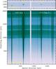 |
Fig. 1 Acquisition images through the 40′′ slit (top panel) and corresponding dispersed two-dimensional spectra (bottom panel) for Runs 2 and 3 obtained with GTC/OSIRIS. We note that Run 1 had a slightly different pointing, where both Ref #1 and Target were placed on CCD chip 1 and the 12′′ slit was used. |
2.1.3. Run 3: the transit on March 10, 2016
This Run had the same instrument configuration as Run 2. The 40′′-wide slit was employed, and two stars were placed on different CCD chips. No moon was present during this observation. The seeing ranged from 0.9′′ to 2.5′′, with a median value of 1.5′′. The seeing-limited spectral resolution was ~12 Å. The position drifts in the spatial and dispersing directions were measured to be within 1 pixel and 0.5 pixel, respectively. The HeAr and Ne arc lamps were measured through the 0.8′′ slit.
2.2. Data reduction
We reduced the acquired GTC/OSIRIS data using the approach described in Chen et al. (2016), which makes use of the standard IRAF1 routines and customized IDL2 scripts. The data reduction process included trimming of overscan region, subtraction of bias structure, correction of flat field, and removal of sky background. For each night, around 40 to 50 individual bias and flat measurements were used to create the master calibration files, respectively. A two-dimensional pixel-to-wavelength transformation map was constructed based on the line identification of the HeAr and Ne arc lamps. After the stars were masked out and the spectral image was mapped into the wavelength space, a sky background model was constructed for each exposure, and then mapped back into the pixel space, where the sky level under the masked star regions was interpolated wavelength-by-wavelength. The cosmic-ray hits were removed by a simple sigma-clipping method in the time domain for each pixel.
The one-dimensional (1D) spectra were extracted using the optimal extraction algorithm (Horne 1986). The aperture size was fixed for all the exposures in a given Run. The optimal aperture was determined by minimizing the standard deviation of the white-color light-curve residuals among the data sets created with various aperture sizes. The adopted aperture diameters were 57 pixels for Run 1, 29 pixels for Run 2, and 22 pixels for Run 3. As the aperture size increases, the aperture-scatter growth curve always drops quickly at very small apertures, and then rises slowly after reaching the lowest scatter. We confirmed that the aperture choices did not affect our results when the aperture-scatter growth curve became stable.
The wavelength solutions for the extracted 1D spectra was calculated by fitting a third order B-spline function3 to the identified arc lines. For a given star, the spectrum of every exposure was cross-correlated with the first exposure to correct position drift in time. The wavelength difference between the target and reference spectra in the same exposure was corrected as well. Furthermore, the wavelength solutions were corrected to match the air wavelengths of specific stellar absorption lines in the still frame. We note that all the corrections were made in the wavelength solutions, instead of directly interpolating the spectra.
The time stamp was extracted from the FITS headers and shifted to the mid-point of each exposure. They were converted to the barycentric Julian date in the barycentric dynamical time standard (BJDTDB) using the IDL procedures written by Eastman et al. (2010). To create a light curve, the pixel range of a requested passband was calculated using the corrected wavelength solution for each exposure. The counts of the complete pixels within this range were directly summed, while those of the edge pixels were fractionally added. After dividing the target flux by the reference flux, the resulting flux ratios were normalized by the out-of-transit level to create the final light-curve products. Finally, we created the white-color light curve in the wavelength range from 435 nm to 755 nm, and a set of spectroscopic light curves whose passbands are shown as a shaded area in Fig. 2. Since the flux level significantly dropped when approaching the shorter wavelength, the spectroscopic passbands were not evenly divided on purpose, to increase the signal-to-noise ratios in the bluer channels.
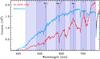 |
Fig. 2 Example stellar spectra of GJ 3470 (red) and its reference star (blue) obtained with GTC/OSIRIS. The color-shaded areas indicate the divided passbands that are used to create spectroscopic light curves. |
2.3. Light-curve analysis
We fit the GTC/OSIRIS transit light curves in the same procedures detailed in Chen et al. (2016). The only difference here is that no third-light contamination exists. Therefore, dilution correction is removed from the fitting procedure. The light-curve data were directly fit with the Mandel & Agol (2002) analytic transit model  multiplied by a systematic decorrelation baseline model ℬ(cj). The potential free parameters in the transit model included the mid-transit time Tmid, the orbital inclination i, the scaled semi-major axis a/R⋆, the planet-to-star radius ratio Rp/R⋆, and the quadratic limb-darkening coefficients (u1, u2). The orbital period P was always fixed to the literature value or the revised value as given below. Since Bonfils et al. (2012) placed a 1-σ upper limit of 0.051 on the orbital eccentricity, the circular orbit was adopted in our analysis. On the other hand, the potential free parameters in the baseline model ℬ(cj) were the coefficients cj for the polynomial combinations of the state vectors s.
The limb-darkening coefficients u1 and u2 were fitted with Gaussian priors. Their theoretical values were interpolated from the ATLAS stellar atmosphere models (Kurucz 1979) using the stellar effective temperature Teff = 3652 ± 50 K, surface gravity log g = 4.78 ± 0.12, and metallicity [Fe/H] = 0.17 ± 0.06 (Biddle et al. 2014). The interpolation was performed using the Python package written by Espinoza & Jordán (2015), where the stellar intensity profiles had been interpolated onto evenly spaced 100-μ (μ = cosθ) grids (Claret & Bloemen 2011). The bandpass response and telluric absorption features have been taken into account in the interpolation. The imposed prior widths were σu = 0.1, which can make use of the known physical information of the host star without imposing too strict constraints.
The initial best-fitting model parameters were determined by the MPFIT package (Markwardt 2009). A customized version of the Transit Analysis Package (TAP; Gazak et al. 2012) was employed to perform the Markov chain Monte Carlo (MCMC) analysis to explore the likelihood distributions of the fitted parameters. This IDL package implements a Metropolis-Hastings MCMC technique within a Gibbs sampler (Ford 2005, 2006). To account for the correlated noise, TAP uses a likelihood function (Carter & Winn 2009) that introduces the Daubechies fourth-order wavelet decomposition and assumes the power spectral density varies as 1 /f at the frequency f. The final reported parameter values and uncertainties were calculated as the median and 1-σ percentiles of each parameter’s likelihood distribution.
2.3.1. Fitting of white-color light curves
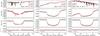 |
Fig. 3 White-color light curves of GJ 3470 obtained with GTC/OSIRIS on January 30 (Run 1; left panel), February 9 (Run 2; middle panel), and March 10 (Run 3; right panel) in 2016. In each panel, from top to bottom are: (1) raw flux time series of the target (black line) and reference (red line) stars; (2) raw light curve (target-to-reference flux ratio; black points) and the best-fitting combined model (red line); (3) corrected light curve after removing the best-fitting systematics model, overplotted with the best-fitting transit model; (4) best-fitting light-curve residuals. |
We first fit the white-color light curves to derive the overall transit parameters. For the GTC/OSIRIS observations, the rotator-angle dependent systematics have been a known issue in the previous studies when the rotator angle φ varies more than ~60° and the stars are far away from the Nasmyth rotator center (e.g., Nortmann et al. 2016; Chen et al. 2016). Such systematics will introduce sinusoid-like features that could distort the observed light curves. As summarized in Table 1, all three GTC/OSIRIS Runs spanned a rotator angle range larger than 90°. The white-color light curves indeed exhibit sinusoid-like trends that cannot be solely described by the polynomial combinations of state vectors. Therefore, we modified the baseline model as: 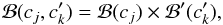 (1)where
  is the sinusoid function.
To determine the optimal baseline model that can well decorrelate systematics, we tested all the polynomial combinations of different state vectors in linear to third-order forms. The state vectors included spectra’s relative position shifts in the spatial and dispersing directions (x, y), spectra’s full-width at the half maximum (FWHM) in the spatial and dispersing directions (sx, sy), airmass z, and time sequence t. We employed the Bayesian information criterion (BIC; Schwarz 1978) to penalize the models that have too many degrees of freedom (d.o.f.). The final selected baseline models for the three Runs are listed below: ![Mathematical equation: \begin{eqnarray} \mathcal{B}_\mathrm{Run\_1} &= & ~(c_0+c_1x+c_2y+c_3y^2+c_4s_y+c_5s_y^2+c_6z)\nonumber\\ && ~\times[1+c^\prime_0\cos(\phi+c^\prime_1)],\\ \mathcal{B}_\mathrm{Run\_2} &= & ~(c_0+c_1y+c_2s_x+c_3s_y+c_4s_y^2+c_5z)\nonumber\\ && ~\times[1+c^\prime_0\cos(c^\prime_1\phi+c^\prime_2)],\\ \mathcal{B}_\mathrm{Run\_3} &= & ~(c_0+c_1y+c_2s_x+c_3s_y+c_4s_x^2+c_5s_y^2+c_6t)\nonumber\\ && ~\times[1+c^\prime_0\cos(c^\prime_1\phi+c^\prime_2)]. \end{eqnarray}](/articles/aa/full_html/2017/04/aa30228-16/aa30228-16-eq64.png) We then performed three analyses for certain purposes:
We then performed three analyses for certain purposes:
-
Firstly, we jointly fit Runs 2 and 3 assuming thatthe free parameters (i, a/R⋆, Rp/R⋆, u1, u2) were common. The mid-transit time Tmid and the coefficients (cj,
 ) of the systematics baseline models were Run dependent. The derived transit parameters are given in Table 2, which are fully consistent with the ones obtained by the Spitzer observations in the 4.5 μm band and other literature studies (see Table 2 of Awiphan et al. 2016).
 -
Secondly, we fixed (i, a/R⋆, Tmid) to the values listed in Table 2 and fit Rp/R⋆ individually. This results in Rp/R⋆ values of 0.0770 ± 0.0024 and 0.0779 ± 0.0022 for Runs 2 and 3, respectively. The transit depth difference is well within the measured uncertainties. Although the impact of the associated instrumental systematics has been included in the large error bars, the best-fitting absolute transit depth value might be biased to some extent. Stellar activity could be another possibility (see the discussion in Sect. 4.2).
-
Thirdly, we derived the mid-transit time for Run 1.
The white-color light curves of the three Runs are shown in Fig. 3. The standard deviation of the normalized residuals are 988 ppm (43 s cadence), 381 ppm (30 s cadence), and 480 ppm (30 s cadence) for Runs 1−3, respectively, which achieved 10.6, 2.4, and 3.1 times of the expected photon noise limits. Using the time-averaging β approach (e.g., Pont et al. 2006; Winn et al. 2008; Gillon et al. 2010), the contribution of correlated noise was estimated as 255 ppm, 298 ppm, and 335 ppm for Runs 1−3, respectively.
2.3.2. Revised transit ephemeris
The three new mid-transit measurements from our GTC/OSIRIS observations are listed in Table 2. To refine the transit period, we also collected the mid-transit times of 13 transits reported in Awiphan et al. (2016) which included three re-analyzed transits of Bonfils et al. (2012), 11 transits reported in Dragomir et al. (2015) which included one re-analyzed transit of Biddle et al. (2014), and nine transits reported in Biddle et al. (2014) which included two re-analyzed transits of Nascimbeni et al. (2013) and Fukui et al. (2013). The separately reported mid-transit times of Crossfield (2013) and Demory et al. (2013) were also included. All the mid-transit times were fitted by the linear function: T(E) = T0 + E × P (see Table 2). The reduced chi-square for this fitting is  , indicating that the linear ephemeris can well describe the current orbit. No significant transit time variation (TTV) is observed under current precision.
Derived parameters for the GTC/OSIRIS observations.
2.3.3. Fitting of spectroscopic light curves
 |
Fig. 4 Raw (left panels) and detrended (right panels) spectroscopic light curves obtained with GTC/OSIRIS for Runs 2 and 3. |
To derive the transmission spectrum for GJ 3470b, we fit the spectroscopic light curves using the following systematics baseline model:  (5)where
  refers to the Run-dependent common-mode systematics derived from the white-color light curves. This model was also selected using the BIC values among a large set of polynomial combinations of state vectors which did not include any sinusoid trends. The common-mode systematics were derived after dividing the white-color light-curve data by the corresponding best-fitting transit model. According to the benchmark test on the transmission spectrum of a transiting white dwarf (Chen et al. 2016), the GTC/OSIRIS rotator-angle dependent systematics are achromatic, and the divide-white method that incorporates the common-mode trends in the baseline models could recover the buried transmission spectrum.
We fixed the values of the common parameters (i, a/R⋆, Tmid) to those obtained in the white-color light curves. The parameters (Rp/R⋆, u1, u2) and baseline coefficients cj were fitted separately for different spectroscopic light curves. The resulting standard deviation of the normalized residuals for the spectroscopic light curves achieved a range of 1.0–1.9 and 1.0–1.7 times of the expected photon noise limits for Runs 2 and 3, respectively. The derived values of Rp/R⋆ in different passbands are given in Table 3. The raw spectroscopic light curves and the detrended ones are shown in Fig. 4. The transmission spectra derived from Runs 2 and 3 are in full agreement with each other, with a chi-square value of χ2 = 5.3 (d.o.f. = 10). If one is allowed to have an overall shift in transit depth to match another, the agreement becomes even better (χ2 = 2.2, d.o.f. = 9). The resulting overall shift is ΔRp/R⋆ = 0.0012, which is consistent with the difference in the white-color light-curve transit depths (ΔRp/R⋆ = 0.0009 ± 0.0033). We also note that the major deviation came from the bluest channel and the reddest channel while the in-between channels exhibited almost the same decreasing trend with increasing wavelengths (see the top panel of Fig. 5).
Measured Rp/R⋆ for the divided GTC/OSIRIS passbands.
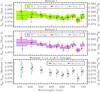 |
Fig. 5 GTC/OSIRIS transmission spectra derived by different methods. Method 1 (top panel) refers to the Bayesian Information Criterion based model selection. Method 2 (middle panel) refers to the Akaike Information Criterion based systematics models marginalization. The single-Run transmission spectra are shown in red and blue for Runs 2 and 3, respectively. The shadowed boxes are the weighted average of the two nights, which are also separately shown in the bottom panel. The two data sets in each panel are shifted in wavelength for clarity. |
Gibson (2014) proposed that marginalization over many systematics is more robust than simple model selection, and that the BIC-based model selection could be the worst criterion in their experiments. To assess the impact of BIC-based model selection choices (hereafter Method 1) on our derived transmission spectrum, we also performed a separate analysis on the spectroscopic light curves employing the systematics marginalization approach (hereafter Method 2). We followed the implication of this approach described in Wakeford et al. (2016), and refer the reader to that work for more details. Instead of using the wavelet-based MCMC to account for the correlated noise (see Method 1), for simplicity, Method 2 employed the MPFIT package to fit the data and accounted for the correlated noise using the time-averaging β approach. We calculated the marginal likelihood for all the systematics models using the Akaike information criterion (AIC; Akaike 1973) as the approximation, that is,  , which provides more adequate fits and performs better than BIC as suggested by Gibson (2014). The resulting Rp/R⋆ in each spectroscopic channel was then calculated as the marginal-likelihood-weighted average of the best-fitting values from all the systematics models, whose uncertainty was propagated from both the deviation from the weighted average and the best-fitting error bar for each systematics model. The derived Rp/R⋆ values are also listed in Table 3. The middle and bottom panels of Fig. 5 show the transmission spectra derived by Method 2 and the comparison between these two methods, respectively. The great consistency confirms that the BIC-based model selection in this work does not bias the derived transmission spectrum. Since the two methods have almost the same transit-depth values in any given spectral channel, we decide to present the results from Method 2 in the following discussion, as they have smaller error bars.
2.3.4. Re-analysis of Nascimbeni et al.’s LBT light curves
For the consistency of our work, we re-analyzed the two LBT transit light curves from Nascimbeni et al. (2013) following Method 1, with a simple baseline model ℬ = c0 + c1t. We fixed the values of P, i, a/R⋆ to those listed in Table 2, and treated the limb-darkening coefficients in the same way as described in Sect. 2.3. The derived planet-to-star radius ratio is 0.0805 ± 0.0021 in the Uspec filter and 0.07488 ± 0.00057 in the F972N20 filter. We will interpret this re-analyzed data together with our GTC/OSIRIS data in Sect. 5.
3. High resolution spectra
3.1. Observations and data reduction
In order to assess the impact of stellar activity on transit observations and to search for narrow spectral signatures in the transmission spectrum, a transit of GJ 3470b was observed with the high resolution Ultraviolet and Visual Echelle Spectrograph (UVES; Dekker et al. 2000) at the ESO’s Very Large Telescope (VLT) in program 096.C-0258(A). The observation was conducted continuously on January 14, 2016 from 04:50 UT to 08:40 UT (JD 2 457 401.701 to JD 2 457 401.861). The flat part of the transit lasted from 05:57 UT to 07:30 UT and the whole transit from 05:47 UT to 07:41 UT. During this time, 22 spectra with exposure times of 568s were obtained. The spectra cover the wavelength range from 325.9 to 449.3 nm in the blue and 472.6 nm to 683.5 nm in the red part. Due to an earthquake on November 27, 2015 of magnitude 6.2, at a distance of ~30 km from Paranal, the resolution of UVES in the blue channel was slightly reduced to λ/ Δλ = 45 000 instead of λ/ Δλ = 55 000 with the 0.8 arcsec slit used. The resolution in the red channel is λ/ Δλ = 52 000. The standard reduction pipeline was used for the data reduction, but the raw spectra were also manually reduced using standard IRAF tools with no effect on the scientific results.
3.2. Results
3.2.1. Change of line flux between in- and out-of-transit
We derived a flux of (0.95 ± 0.002) × 10-14erg cm-2 s-1, and (1.22 ± 0.008) × 10-14erg cm-2 s-1 for the Ca ii H and K lines, respectively. With a distance of 28.8 ± 2.5 pc (Biddle et al. 2014), this gives log (Ca ii H+K) = 5.15 ± 0.21 (cgs).
Figure 6 shows the lines of Ca ii H+K and Hα taken in- and out-of-transit. The difference is so small that it can hardly be seen. The blue line below shows the ratio of the in-transit to the out-of-transit spectrum. The relative flux of the Ca ii H+K emission cores changes by only 0.67 ± 0.22%. Because M-stars are very faint in the UV, the Hα line is often used as activity indicator. Again, there is no significant difference seen in the in- and out-of-transit spectrum. The relative flux change is even smaller for Hα, only 0.21 ± 0.19%, and thus no significant change of the line flux, or equivalent width, are found.
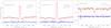 |
Fig. 6 GJ 3470’s Ca ii H (left), Ca ii K, (middle) and Hα (right) in- (black) and out-of-transit (red). The blue line is the ratio between the two. |
3.2.2. High-resolution transmission spectra
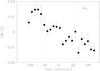 |
Fig. 7 Equivalent width of the Hα transmission spectrum. The dashed lines indicate the beginning and the end of the transit, |
As pointed out by Cauley et al. (2016), the Ca ii H+K lines can be used to find out if any pre-transit Balmer line signal is caused by stellar activity or by material escaping from the planet. The transmission spectrum of planetary atmosphere is defined as:  (6)and the equivalent width of the transmission spectrum is defined as the integral from −200 km s-1 to + 200 km s-1:
  (7)In order to study the planetary atmosphere or the material that might be escaping from the planet, we derived the transmission spectrum in the Na i D1, Na i D2, Hα, and tried to find out if there are effects from the stellar activity in Ca ii H+K. The equivalent width variations of Hα are shown in Fig. 7. The planetary atmosphere would cause an absorption feature during the transit that is not seen before or after the transit. However, we observed a constant decrease in Hα and an increase in the Ca ii H+K lines. The equivalent widths of the Ca ii H+K and Hα transmission spectra are well correlated, with a correlation factor of −0.85. Given that Hα is an absorption line and Ca ii H+K are emission lines, the best explanation is that the change of the equivalent width is caused by a small decrease of the active regions that are visible on the stellar surface. However, this effect is tiny (see Table 4) compared to those of the stellar atmosphere, as stellar Hα has an equivalent width of 0.411 ± 0.017 Å, stellar Ca ii H has −3.558 ± 0.048 Å, and stellar Ca ii K has −5.432 ± 0.063 Å. Thus the change of the active regions’ size is quite small and can be explained simply by active regions that rotate out of view. There is no significant change of the Na lines during the transit. We thus conclude that we did not detect the planetary atmosphere in the Balmer, Ca ii, and Na lines.
Equivalent widths of the Hα, Na i and Ca ii transmission spectra.
4. Stellar activity
4.1. Chromospheric activity
The plage regions are characterized by the chromospheric emission cores in the resonance lines like Ca ii H+K and Mg ii h+k. With the emission flux of Ca ii H+K lines obtained in Sect. 3.2.1, we can derive the magnetic filling factor, which is defined as the fraction of the stellar surface covered by magnetic fields.
Martínez-Arnáiz et al. (2011) determined the fluxes in the Ca ii H+K lines for magnetically saturated stars using high-resolution spectra. They derived log (Ca ii H+K) values of 6.01 ± 0.07 (cgs) for V105 Or (M1.5V) and 6.00 ± 0.03 (cgs) for V371 Ori (M2V). Since the magnetic filling factor of these stars has to be no more than 100%, this gives us an upper limit of the magnetic filling factor of ~15% for GJ 3470. Fawzy et al. (2002) calculated theoretically the heating of the chromosphere and the fluxes in the Ca ii H+K lines for stars of different spectral type. By rescaling these values to the observed fluxes in the Ca ii H+K lines, they derived a relation between the fluxes of these lines and the magnetic filling factor. If we use the fluxes obtained with high-resolution spectra as published by Martínez-Arnáiz et al. (2011) and this model, we can roughly estimate that the magnetic filling factor of GJ 3470 is larger than ~10%. The Ca ii H+K filling factor on the Sun varies typically within 1–9% from the solar minimum to the maximum (Meunier & Delfosse 2009). In this sense, with a filling factor of 10−15%, GJ 3470 is more active than the Sun.
Given that the planet occults only 0.6% of the stellar surface, this large filling factor means that it is impossible for the planet to occult all the plage regions at any one moment. Therefore, only when the plage regions are disproportionally occulted, that is if they are preferentially located along the path of the planet, would we see a significant decrease of the emission line flux of Ca ii H+K. Since it only changes by 0.67 ± 0.22%, the plage regions are likely very homogeneously distributed over the stellar surface.
4.2. Photospheric activity
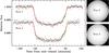 |
Fig. 8 Modeling the light curves with the assumption of occulted spots. The red and green lines show the spotted transit model and non-spotted transit model, respectively. |
While high-resolution spectroscopy can probe active regions in the chromosphere (e.g., plages), white-color light curves can provide information of star spots that are originating from the photosphere. Our GTC/OSIRIS white-color light curves showed a small offset in planet-to-star ratios between Runs 2 (0.0770 ± 0.0024) and 3 (0.0779 ± 0.0022), which could be caused by either observational systematics or the impact of stellar activity. Due to the normalization effect in the light-curve modeling process, the apparent transit depth would change from epoch to epoch due to the modulation of star spots. According to the photometric monitoring by Fukui et al. (2013) and Biddle et al. (2014), GJ 3470 did show a peak-to-valley amplitude of ~1% with a rotational period of 20.7 ± 0.15 days.
Given that the bump-like time-correlated noise could come from occulted dark star spots, we re-modeled the GTC/OSIRIS light curves with the PRISM+GEMC code (Tregloan-Reed et al. 2013, 2015), which uses a pixellation approach in Cartesian coordinates to generate the spotted transit light curve (see Fig. 8). The fitted spot angular radius and contrast were 4.3° ± 11.8° and 0.45 ± 0.23 for Run 2, and 8.9° ± 10.1° and 0.75 ± 0.44 for Run 3. Using the PHOENIX stellar atmosphere models (Husser et al. 2013) and GTC/OSIRIS response, we found that the spots were  K and
K and  K cooler than the photosphere (Tspot = 3652 K), respectively. The spot-photosphere temperature differences are in line with the decreasing trend as a function of decreasing photosphere temperature (e.g., Berdyugina 2005; Andersen & Korhonen 2015). Assuming that the stellar variability is also 1% in our GTC/OSIRIS passband and that any unocculted star spots have similar contrast, the spot filling factors would be 1.8 ± 0.8% and 4 ± 7% for Runs 2 and 3, which are clearly smaller than the magnetic filling factor (10–15%). The spot filling factor has been found to be strongly deviating from and smaller than the magnetic filling factor for cool late-type stars, suggesting that they refer to different activity signatures (Berdyugina 2005).
These time-correlated noises could in principle also be modeled by occulted bright spots. In that case, a minimum spot filling factor of 36 ± 14% and 49 ± 10% is derived for Runs 2 and 3, respectively. The fitted contrasts of 1.33 ± 0.11 and 1.23 ± 0.07 indicate that these spots are 154 ± 46 K and 109 ± 32 K hotter than the photosphere, respectively. This would translate into a flux variability larger than ~12%, which strongly disagrees with the long-term monitoring photometry. Furthermore, introducing occulted bright spots would make the real transit depth much shallower and more discrepant from the infrared transit observations. Therefore, the scenario of occulted bright spots is unlikely to be the cause of the correlated noise.
4.3. Impact of stellar activity on transmission spectrum
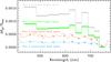 |
Fig. 9 Impact of stellar activity on a flat constant line. These apparent relative transmission spectra were calculated using the fitting results obtained in Sect. 4.2 for the cases of unocculted dark spots (lines with diamonds) and occulted bright spots (histogram lines), respectively. |
We now attempt to assess the impact of stellar activity on the derived transmission spectrum in a single epoch. The occulted dark star spots discussed in Sect. 4.2, if they were real, exhibited non-detectable wavelength dependent variation, thus having negligible impact on the transmission spectrum.
For the impact of unocculted dark star spots, we calculated the apparent transit depths  using Eq. (1) presented in McCullough et al. (2014):
 ![Mathematical equation: \begin{eqnarray} \frac{\tilde{R}^2_\mathrm{p}}{\tilde{R}^2_\star} = \frac{R^2_\mathrm{p}}{R^2_\star}\frac{1}{1-\delta[1-F_\nu({\mathrm{spot}})/F_\nu({\mathrm{phot}})]}, \end{eqnarray}](/articles/aa/full_html/2017/04/aa30228-16/aa30228-16-eq146.png) (8)where Fν(spot) and Fν(phot) are the spectra of the spots and the photosphere, respectively, and δ is the spot filling factor. We adopted the PHOENIX stellar atmosphere models, and used the spot filling factors and spot temperatures determined in Sect. 4.2. As shown in Fig. 9, if there were unocculted dark star spots, a flat spectrum at the constant value of Rp/R⋆ = 0.0777 would appear to be wavelength dependent in the measurements. Due to strong absorption bands of TiO/VO in the cool stellar atmosphere, the apparent transmission spectrum binned in our passbands is relatively flat in the wavelengths 435–735 nm rather than mimicking a Rayleigh scattering slope, where the maximum differences are only ΔRp/R⋆ = 0.00008 and 0.00018 for Runs 2 and 3, respectively. The apparent planetary radius is much smaller in the 735–755 nm band, making the relative spectral shape more deviating from a potential Rayleigh scattering slope and our measurements.
(8)where Fν(spot) and Fν(phot) are the spectra of the spots and the photosphere, respectively, and δ is the spot filling factor. We adopted the PHOENIX stellar atmosphere models, and used the spot filling factors and spot temperatures determined in Sect. 4.2. As shown in Fig. 9, if there were unocculted dark star spots, a flat spectrum at the constant value of Rp/R⋆ = 0.0777 would appear to be wavelength dependent in the measurements. Due to strong absorption bands of TiO/VO in the cool stellar atmosphere, the apparent transmission spectrum binned in our passbands is relatively flat in the wavelengths 435–735 nm rather than mimicking a Rayleigh scattering slope, where the maximum differences are only ΔRp/R⋆ = 0.00008 and 0.00018 for Runs 2 and 3, respectively. The apparent planetary radius is much smaller in the 735–755 nm band, making the relative spectral shape more deviating from a potential Rayleigh scattering slope and our measurements.
Since the maximum difference of the apparent planetary radius in the GTC/OSIRIS passband is much smaller than the average radius ratio uncertainty, this impact plays a negligible role in changing the shape of the observed transmission spectrum. Therefore, we conclude that (i) the variation in the transmission spectrum of our single Run, and (ii) the difference between the transmission spectra of our two Runs, are not likely caused by the unocculted dark star spots. However, it should be noted that the spot spectrum does not necessarily follow the same as the photosphere. Sing et al. (2011) analyzed the wavelength dependent effect of the occulted star spots in HD 189733b, and found that the expected MgH feature at the wavelength 500 nm was weaker than expected. In our case, it is still possible that an ad hoc spot spectrum happens to cancel out all the TiO/VO bands to show a Rayleigh scattering like slope. But this is beyond the scope of this discussion.
Oshagh et al. (2014) have attempted to use occulted bright spots to explain the transmission spectrum of GJ 3470b. This worked well if blackbody emission is assumed for both bright spots and photosphere. Here we again adopted the PHOENIX stellar atmosphere models, and simply assumed that the bright spots were 100 K hotter than the photosphere. The location and size of the occulted bright spots were inherited from the fitting results determined in Sect. 4.2. Synthetic spotted light curves were created using the spot-to-photosphere flux ratios in the corresponding passbands, and then were fitted by the non-spotted transit model to derive the final apparent transmission spectrum. As shown in Fig. 9, the apparent transmission spectrum resulting from occulted bright spots would introduce similar relative variation to that from the unocculted dark spots, but in a larger scale. The same conclusion as the unocculted dark spots also applies to the occulted bright spots. On the other hand, according to the discussion in Sect. 4.2, we also emphasize that the occulted bright spots are not likely present in our observed light curves.
5. Interpreting the transmission spectrum as planetary atmosphere
For the discussion in this section, we calculated a weighted average GTC/OSIRIS transmission spectrum after shifting upwards ΔRp/R⋆ = 0.00115 to let Run 2 match Run 3. The change of the relative shape of transmission spectrum caused by stellar activity is assumed to be negligible. The average transmission spectrum is also presented in Table 3.
5.1. Spectrally-resolved scattering slope
As shown in Fig. 10, our derived GTC/OSIRIS transmission spectrum shows a clear trend of decreasing planetary radii with increasing wavelengths. Therefore, we performed a linear fit to this trend in the (lnλ, Rp/R⋆) space, and derived a slope of −0.0032 ± 0.0016 (χ2 = 11.2; d.o.f. = 8). According to Lecavelier Des Etangs et al. (2008), if the opacity sources in the planetary atmosphere have a cross section in the form of σ = σ0(λ/λ0)α, a slope would be introduced into the transmission spectrum, which is connected to the atmospheric scale height H: 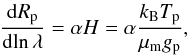 (9)where kB is the Boltzmann constant, Tp and μm are the temperature and mean molecular weight of the planetary atmosphere, respectively, and gp is the planetary surface gravity. For GJ 3470b, we obtained gp = 6.8 ± 1.7 m s-2, R⋆ = 0.48 ± 0.04 R⊙, and Teff = 3652 ± 50 K from Biddle et al. (2014), and calculated a new equilibrium temperature as Tp = (1−AB)1/4 × (711 ± 25) K. The Bond albedo AB could be zero for a dark surface in the extreme case. The typical value for Uranus and Neptune4 in our Solar system is 0.3.
According to our fitting result, if GJ 3470b’s atmosphere is composed of solar-composition hydrogen and helium dominated atmosphere (i.e., μm = 2.37), the slope in the cross section would be α = −2.9 ± 1.6 (AB = 0.0) or α = −3.2 ± 1.8 (AB = 0.3), which covers the Rayleigh scattering slope α = −4 within the error bar. On the other hand, if Rayleigh scattering is assumed, a mean molecular weight of μm = 3.3 ± 1.8 (AB = 0.0) or μm = 2.9 ± 1.7 (AB = 0.3) would be required for the atmosphere, which is slightly heavier than the solar-composition hydrogen-helium atmosphere.
Nascimbeni et al. (2013)’s LBT observations were conducted in two filters either bluer or redder than our GTC/OSIRIS wavelength range. Neglecting the impact of stellar activity, if the two re-analyzed LBT measurements are included in our aforementioned fitting, we would derive a slope of −0.0049 ± 0.0010. This corresponds to a cross-section slope of α = −4.5 ± 1.5 (AB = 0.0, μm = 2.37) or α = −4.9 ± 1.7 (AB = 0.3, μm = 2.37), which is still consistent with but slightly steeper than the Rayleigh scattering slope.
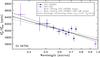 |
Fig. 10 Optical transmission spectrum of GJ 3470b. The GTC/OSIRIS measurements and re-analyzed LBT/LBC measurements are shown in navy-blue circles and purple squares with error bars, respectively. The dotted line shows the best-fitting slope of the GTC/OSIRIS measurements. The dashed line shows the best-fitting slope of the combined GTC/OSIRIS and LBT/LBC measurements. The solid line shows a Rayleigh scattering slope based on the physical parameters of GJ 3470b with a mean molecular weight of μm = 2.37 and a Bond albedo of AB = 0.3. |
5.2. Transmission spectroscopy as a whole
The transmission spectra of GJ 3470b have also been obtained by HST/WFC3 in the 1.1–1.7 μm band (Ehrenreich et al. 2014) and by Keck/MOSFIRE in the 2.09–2.36 μm band (Crossfield et al. 2013). These two near-infrared transmission spectra have the same overall transit-depth level, and both indicate a flat featureless spectrum originating from high-altitude clouds or high metallicity atmospheric compositions. Ehrenreich et al. (2014) discussed in depth the prompted dichotomic spectrum when collecting the optical photometric measurements together with the near-infrared transmission spectrum. They found that the combination of the tentative Rayleigh scattering slope in the optical and the flat featureless spectrum in the near-infrared had to be explained by a cloudy hydrogen-rich atmosphere with an extremely low water volume mixing ratio, which, however, were not necessarily physically or chemically realistic (e.g., Hu & Seager 2014).
When comparing to the HST/WFC3 near-infrared transmission spectrum, the GTC/OSIRIS and LBT/LBC combined optical transmission spectrum is clearly slightly downwards offset (see the top panel of Fig. 11). Planets with larger infrared radii than the optical would indicate predominantly clear atmospheres (e.g., Sing et al. 2016). However, in the case of GJ 3470b, the infrared measurements might suggest a cloudy atmosphere or a pure water atmosphere. While the Rayleigh scattering slope is spectroscopically confirmed, it is difficult to explain this optical trend that goes into atmospheric layers deeper than the cloud deck or the pure water absorption suggested by the infrared data. We note that the GTC/OSIRIS + LBT/LBC spectrum, except for the one in the F972N20 filter, well matches the prediction of a cloudy hydrogen-rich atmosphere (i.e., the blue model in the top panel of Fig. 11; taken from Ehrenreich et al. 2014) if they had been moved upwards  ppm.
ppm.
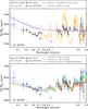 |
Fig. 11 Transmission spectrum of GJ 3470b, which includes the transit depth measurements from GTC/OSIRIS (navy-blue circles), LBT/LBC (purple squares), HST/WFC3 (black diamonds), and Keck/MOSFIRE (black triangles). The two models shown in the top panel are taken from Ehrenreich et al. (2014), which correspond to H2-rich atmospheres with 1 ppm H2O and clouds at 100 mbar (blue) or with 1% H2O and no clouds (orange), respectively. The three models shown in the bottom panel are computed using the Exo-Transmit code (Kempton et al. 2017). In the top panel, the GTC/OSIRIS+LBT/LBC measurements are shifted upwards 343 ppm, and then shown as empty symbols in gray. |
While stellar activity remains a possibility to introduce an offset between data sets obtained at different epochs, we also note that our GTC/OSIRIS transmission spectrum is compatible with the HST/WFC3 measurements. In the bottom panel of Fig. 11, we show three atmospheric models computed using the Exo-Transmit code (Kempton et al. 2017): (1) a 700 K cloud-free model with 0.1× solar composition; (2) a 500 K cloud-free model with 0.1× solar composition; (3) a 700 K model with 100× solar composition and 50× enhanced Rayleigh scattering. Comparing these three models to the GTC/OSIRIS and HST/WFC3 combined data sets, the reduced chi-squares  are 1.60, 1.19, and 1.17, respectively. In contrast, a horizontal line would result in
  . This indicates that the combination of lower temperature and lower metallicity in a cloud-free atmosphere can reduce the near-infrared spectral modulation while keeping a slope similar to the one suggested by the optical data. Similarly, it can also be achieved by higher metallicity with enhanced Rayleigh scattering from hazes. With the current data collection, the compositions of GJ 3470b’s atmosphere are still degenerate. We expect that the atmosphere of GJ 3470b can be well constrained in the future with more transit spectroscopy observations at higher precision, hopefully simultaneously in the optical and infrared.
6. Conclusions
We have observed three transits of the warm sub-Uranus-mass planet GJ 3470b with GTC/OSIRIS in low-resolution spectroscopy. While the first transit was performed in extremely poor weather conditions, the remaining two transits allowed us to obtain the first high-quality transmission spectrum in the wavelength range 435−755 nm. We were able to spectrally-resolve the Rayleigh scattering slope in GJ 3470b’s atmosphere for the first time.
We have also observed one transit of GJ 3470b with VLT/UVES in high-resolution spectroscopy. We found that GJ 3470 is an active star with a magnetic filling factor of around 10–15%. The relative flux of the emission cores of the Ca ii H+K lines changes by only 0.67 ± 0.22% in- and out-of-transit. The relative flux of the Hα lines changes by only 0.21 ± 0.19%. We have not statistically detected any narrow absorption signatures originating from the planetary atmosphere.
Combining the low- and high-resolution spectroscopy, we have discussed the possible impacts from stellar activity. With current knowledge of the host star, the transmission spectrum is not likely to be significantly contaminated by the wavelength dependent effect from stellar activity. However, an overall shift from epoch to epoch caused by stellar activity is still possible. Therefore, a better observing strategy for future transmission spectroscopy of this planet would be a large wavelength coverage encompassed by a long-term photometric monitoring campaign.
IRAF is distributed by the National Optical Astronomy Observatory, which is operated by the Association of Universities for Research in Astronomy (AURA) under a cooperative agreement with the National Science Foundation.
IDL stands for Interactive Data Language. It is a registered trademark of Exelis Inc. For further details see: http://www.exelisvis.com/ProductsServices/IDL.aspx
Acknowledgments
We thank the anonymous referee for his/her careful reading and helpful comments that improved the manuscript. We thank Dr. D. Ehrenreich for kindly providing us with the theoretical atmospheric models. This research is based on observations made with the Gran Telescopio Canarias (GTC), installed in the Spanish Observatorio del Roque de los Muchachos, operated on the island of La Palma by the Instituto de Astrofísica de Canarias. This work is partly financed by the Spanish Ministry of Economics and Competitiveness through projects ESP2013-48391-C4-2-R, ESP2014-57495-C2-1-R, and AYA2012-39346-C02-02. This work was supported by the Thüringer Ministerium für Wirtschaft, Wissenschaft und Digitale Gesellschaft. G.C. also acknowledges the support by the National Natural Science Foundation of China (Grant No. 11503088) and the Natural Science Foundation of Jiangsu Province (Grant No. BK20151051). This research has made use of the VizieR catalogue access tool, CDS, Strasbourg, France (Wenger et al. 2000).
References
- Akaike, H. 1973, in 2nd International Symposium on Information Theory, eds. B. N. Petrov, & F. Csaki, 267 [Google Scholar]
- Andersen, J. M., & Korhonen, H. 2015, MNRAS, 448, 3053 [NASA ADS] [CrossRef] [Google Scholar]
- Awiphan, S., Kerins, E., Pichadee, S., et al. 2016, MNRAS, 463, 2574 [NASA ADS] [CrossRef] [Google Scholar]
- Bailey, J. 2014, PASA, 31, e043 [NASA ADS] [CrossRef] [Google Scholar]
- Bean, J. L., Miller-Ricci Kempton, E., & Homeier, D. 2010, Nature, 468, 669 [NASA ADS] [CrossRef] [PubMed] [Google Scholar]
- Bean, J. L., Désert, J.-M., Kabath, P., et al. 2011, ApJ, 743, 92 [NASA ADS] [CrossRef] [Google Scholar]
- Berdyugina, S. V. 2005, Liv. Rev. Sol. Phys., 2, 8 [Google Scholar]
- Berta, Z. K., Charbonneau, D., Désert, J.-M., et al. 2012, ApJ, 747, 35 [NASA ADS] [CrossRef] [Google Scholar]
- Biddle, L. I., Pearson, K. A., Crossfield, I. J. M., et al. 2014, MNRAS, 443, 1810 [NASA ADS] [CrossRef] [Google Scholar]
- Bonfils, X., Gillon, M., Udry, S., et al. 2012, A&A, 546, A27 [NASA ADS] [CrossRef] [EDP Sciences] [Google Scholar]
- Carter, J. A., & Winn, J. N. 2009, ApJ, 704, 51 [NASA ADS] [CrossRef] [Google Scholar]
- Cauley, P. W., Redfield, S., Jensen, A. G., & Barman, T. 2016, AJ, 152, 20 [NASA ADS] [CrossRef] [Google Scholar]
- Charbonneau, D., Brown, T. M., Latham, D. W., & Mayor, M. 2000, ApJ, 529, L45 [NASA ADS] [CrossRef] [PubMed] [Google Scholar]
- Charbonneau, D., Brown, T. M., Noyes, R. W., & Gilliland, R. L. 2002, ApJ, 568, 377 [NASA ADS] [CrossRef] [Google Scholar]
- Charbonneau, D., Allen, L. E., Megeath, S. T., et al. 2005, ApJ, 626, 523 [NASA ADS] [CrossRef] [Google Scholar]
- Chen, G., Palle, E., Murgas, F., et al. 2016, A&A, submitted (Paper VII) [Google Scholar]
- Claret, A., & Bloemen, S. 2011, A&A, 529, A75 [NASA ADS] [CrossRef] [EDP Sciences] [Google Scholar]
- Crossfield, I. J. M. 2013, A&A, 551, A99 [NASA ADS] [CrossRef] [EDP Sciences] [Google Scholar]
- Crossfield, I. J. M., Barman, T., Hansen, B. M. S., & Howard, A. W. 2013, A&A, 559, A33 [NASA ADS] [CrossRef] [EDP Sciences] [Google Scholar]
- Dekker, H., D’Odorico, S., Kaufer, A., Delabre, B., & Kotzlowski, H. 2000, in Optical and IR Telescope Instrumentation and Detectors, eds. M. Iye, & A. F. Moorwood, Proc. SPIE, 4008, 534 [Google Scholar]
- Deming, D., Seager, S., Richardson, L. J., & Harrington, J. 2005, Nature, 434, 740 [NASA ADS] [CrossRef] [PubMed] [Google Scholar]
- Demory, B.-O., Torres, G., Neves, V., et al. 2013, ApJ, 768, 154 [NASA ADS] [CrossRef] [Google Scholar]
- de Wit, J., Wakeford, H. R., Gillon, M., et al. 2016, Nature, 537, 69 [NASA ADS] [CrossRef] [Google Scholar]
- Dragomir, D., Benneke, B., Pearson, K. A., et al. 2015, ApJ, 814, 102 [NASA ADS] [CrossRef] [Google Scholar]
- Dressing, C. D., & Charbonneau, D. 2013, ApJ, 767, 95 [NASA ADS] [CrossRef] [Google Scholar]
- Eastman, J., Siverd, R., & Gaudi, B. S. 2010, PASP, 122, 935 [NASA ADS] [CrossRef] [Google Scholar]
- Ehrenreich, D., Bonfils, X., Lovis, C., et al. 2014, A&A, 570, A89 [NASA ADS] [CrossRef] [EDP Sciences] [Google Scholar]
- Espinoza, N., & Jordán, A. 2015, MNRAS, 450, 1879 [NASA ADS] [CrossRef] [Google Scholar]
- Fawzy, D., Ulmschneider, P., Stȩpień, K., Musielak, Z. E., & Rammacher, W. 2002, A&A, 386, 983 [NASA ADS] [CrossRef] [EDP Sciences] [Google Scholar]
- Ford, E. B. 2005, AJ, 129, 1706 [Google Scholar]
- Ford, E. B. 2006, ApJ, 642, 505 [NASA ADS] [CrossRef] [Google Scholar]
- Fraine, J., Deming, D., Benneke, B., et al. 2014, Nature, 513, 526 [NASA ADS] [CrossRef] [Google Scholar]
- Fressin, F., Torres, G., Charbonneau, D., et al. 2013, ApJ, 766, 81 [NASA ADS] [CrossRef] [Google Scholar]
- Fukui, A., Narita, N., Kurosaki, K., et al. 2013, ApJ, 770, 95 [NASA ADS] [CrossRef] [Google Scholar]
- Gazak, J. Z., Johnson, J. A., Tonry, J., et al. 2012, Adv. Astron., 2012, 30 [Google Scholar]
- Gibson, N. P. 2014, MNRAS, 445, 3401 [NASA ADS] [CrossRef] [Google Scholar]
- Gillon, M., Lanotte, A. A., Barman, T., et al. 2010, A&A, 511, A3 [NASA ADS] [CrossRef] [EDP Sciences] [Google Scholar]
- Henry, G. W., Marcy, G. W., Butler, R. P., & Vogt, S. S. 2000, ApJ, 529, L41 [NASA ADS] [CrossRef] [PubMed] [Google Scholar]
- Horne, K. 1986, PASP, 98, 609 [NASA ADS] [CrossRef] [EDP Sciences] [Google Scholar]
- Howard, A. W., Marcy, G. W., Bryson, S. T., et al. 2012, ApJS, 201, 15 [NASA ADS] [CrossRef] [Google Scholar]
- Hu, R., & Seager, S. 2014, ApJ, 784, 63 [NASA ADS] [CrossRef] [Google Scholar]
- Husser, T.-O., Wende-von Berg, S., Dreizler, S., et al. 2013, A&A, 553, A6 [NASA ADS] [CrossRef] [EDP Sciences] [Google Scholar]
- Kempton, E. M.-R., Lupu, R. E., Owusu-Asare, A., Slough, P., & Cale, B. 2017, PASP, 129, 044402 [NASA ADS] [CrossRef] [Google Scholar]
- Knutson, H. A., Charbonneau, D., Allen, L. E., et al. 2007, Nature, 447, 183 [NASA ADS] [CrossRef] [PubMed] [Google Scholar]
- Knutson, H. A., Benneke, B., Deming, D., & Homeier, D. 2014a, Nature, 505, 66 [NASA ADS] [CrossRef] [Google Scholar]
- Knutson, H. A., Dragomir, D., Kreidberg, L., et al. 2014b, ApJ, 794, 155 [NASA ADS] [CrossRef] [Google Scholar]
- Kreidberg, L., Bean, J. L., Désert, J.-M., et al. 2014, Nature, 505, 69 [NASA ADS] [CrossRef] [Google Scholar]
- Kurucz, R. L. 1979, ApJS, 40, 1 [NASA ADS] [CrossRef] [Google Scholar]
- Lecavelier Des Etangs, A., Pont, F., Vidal-Madjar, A., & Sing, D. 2008, A&A, 481, L83 [NASA ADS] [CrossRef] [Google Scholar]
- Mandel, K., & Agol, E. 2002, ApJ, 580, L171 [NASA ADS] [CrossRef] [Google Scholar]
- Markwardt, C. B. 2009, in Astronomical Data Analysis Software and Systems XVIII, eds. D. A. Bohlender, D. Durand, & P. Dowler, ASP Conf. Ser., 411, 251 [Google Scholar]
- Martínez-Arnáiz, R., López-Santiago, J., Crespo-Chacón, I., & Montes, D. 2011, MNRAS, 414, 2629 [NASA ADS] [CrossRef] [Google Scholar]
- McCullough, P. R., Crouzet, N., Deming, D., & Madhusudhan, N. 2014, ApJ, 791, 55 [NASA ADS] [CrossRef] [Google Scholar]
- Meunier, N., & Delfosse, X. 2009, A&A, 501, 1103 [NASA ADS] [CrossRef] [EDP Sciences] [Google Scholar]
- Nascimbeni, V., Piotto, G., Pagano, I., et al. 2013, A&A, 559, A32 [NASA ADS] [CrossRef] [EDP Sciences] [Google Scholar]
- Nortmann, L., Pallé, E., Murgas, F., et al. 2016, A&A, 594, A65 [NASA ADS] [CrossRef] [EDP Sciences] [Google Scholar]
- Oshagh, M., Santos, N. C., Ehrenreich, D., et al. 2014, A&A, 568, A99 [NASA ADS] [CrossRef] [EDP Sciences] [Google Scholar]
- Pont, F., Zucker, S., & Queloz, D. 2006, MNRAS, 373, 231 [NASA ADS] [CrossRef] [Google Scholar]
- Rogers, L. A., Bodenheimer, P., Lissauer, J. J., & Seager, S. 2011, ApJ, 738, 59 [NASA ADS] [CrossRef] [Google Scholar]
- Sánchez, B., Aguiar-González, M., Barreto, R., et al. 2012, in SPIE Conf. Ser., 8446, 4 [Google Scholar]
- Schwarz, G. 1978, Ann. Stat., 6, 461 [NASA ADS] [CrossRef] [MathSciNet] [Google Scholar]
- Seager, S., & Deming, D. 2010, ARA&A, 48, 631 [NASA ADS] [CrossRef] [Google Scholar]
- Sing, D. K., Pont, F., Aigrain, S., et al. 2011, MNRAS, 416, 1443 [NASA ADS] [CrossRef] [Google Scholar]
- Sing, D. K., Fortney, J. J., Nikolov, N., et al. 2016, Nature, 529, 59 [NASA ADS] [CrossRef] [Google Scholar]
- Tregloan-Reed, J., Southworth, J., & Tappert, C. 2013, MNRAS, 428, 3671 [NASA ADS] [CrossRef] [Google Scholar]
- Tregloan-Reed, J., Southworth, J., Burgdorf, M., et al. 2015, MNRAS, 450, 1760 [NASA ADS] [CrossRef] [Google Scholar]
- Tsiaras, A., Rocchetto, M., Waldmann, I. P., et al. 2016, ApJ, 820, 99 [NASA ADS] [CrossRef] [Google Scholar]
- Wakeford, H. R., Sing, D. K., Evans, T., Deming, D., & Mandell, A. 2016, ApJ, 819, 10 [NASA ADS] [CrossRef] [Google Scholar]
- Wenger, M., Ochsenbein, F., Egret, D., et al. 2000, A&AS, 143, 9 [NASA ADS] [CrossRef] [EDP Sciences] [Google Scholar]
- Winn, J. N., Holman, M. J., Torres, G., et al. 2008, ApJ, 683, 1076 [NASA ADS] [CrossRef] [Google Scholar]
- Youdin, A. N. 2011, ApJ, 742, 38 [NASA ADS] [CrossRef] [Google Scholar]
- Zacharias, N., Finch, C., Subasavage, J., et al. 2015, AJ, 150, 101 [NASA ADS] [CrossRef] [Google Scholar]
All Tables
All Figures
|
Fig. 1 Acquisition images through the 40′′ slit (top panel) and corresponding dispersed two-dimensional spectra (bottom panel) for Runs 2 and 3 obtained with GTC/OSIRIS. We note that Run 1 had a slightly different pointing, where both Ref #1 and Target were placed on CCD chip 1 and the 12′′ slit was used. |
| In the text | |
|
Fig. 2 Example stellar spectra of GJ 3470 (red) and its reference star (blue) obtained with GTC/OSIRIS. The color-shaded areas indicate the divided passbands that are used to create spectroscopic light curves. |
| In the text | |
|
Fig. 3 White-color light curves of GJ 3470 obtained with GTC/OSIRIS on January 30 (Run 1; left panel), February 9 (Run 2; middle panel), and March 10 (Run 3; right panel) in 2016. In each panel, from top to bottom are: (1) raw flux time series of the target (black line) and reference (red line) stars; (2) raw light curve (target-to-reference flux ratio; black points) and the best-fitting combined model (red line); (3) corrected light curve after removing the best-fitting systematics model, overplotted with the best-fitting transit model; (4) best-fitting light-curve residuals. |
| In the text | |
|
Fig. 4 Raw (left panels) and detrended (right panels) spectroscopic light curves obtained with GTC/OSIRIS for Runs 2 and 3. |
| In the text | |
|
Fig. 5 GTC/OSIRIS transmission spectra derived by different methods. Method 1 (top panel) refers to the Bayesian Information Criterion based model selection. Method 2 (middle panel) refers to the Akaike Information Criterion based systematics models marginalization. The single-Run transmission spectra are shown in red and blue for Runs 2 and 3, respectively. The shadowed boxes are the weighted average of the two nights, which are also separately shown in the bottom panel. The two data sets in each panel are shifted in wavelength for clarity. |
| In the text | |
|
Fig. 6 GJ 3470’s Ca ii H (left), Ca ii K, (middle) and Hα (right) in- (black) and out-of-transit (red). The blue line is the ratio between the two. |
| In the text | |
|
Fig. 7 Equivalent width of the Hα transmission spectrum. The dashed lines indicate the beginning and the end of the transit, |
| In the text | |
|
Fig. 8 Modeling the light curves with the assumption of occulted spots. The red and green lines show the spotted transit model and non-spotted transit model, respectively. |
| In the text | |
|
Fig. 9 Impact of stellar activity on a flat constant line. These apparent relative transmission spectra were calculated using the fitting results obtained in Sect. 4.2 for the cases of unocculted dark spots (lines with diamonds) and occulted bright spots (histogram lines), respectively. |
| In the text | |
|
Fig. 10 Optical transmission spectrum of GJ 3470b. The GTC/OSIRIS measurements and re-analyzed LBT/LBC measurements are shown in navy-blue circles and purple squares with error bars, respectively. The dotted line shows the best-fitting slope of the GTC/OSIRIS measurements. The dashed line shows the best-fitting slope of the combined GTC/OSIRIS and LBT/LBC measurements. The solid line shows a Rayleigh scattering slope based on the physical parameters of GJ 3470b with a mean molecular weight of μm = 2.37 and a Bond albedo of AB = 0.3. |
| In the text | |
|
Fig. 11 Transmission spectrum of GJ 3470b, which includes the transit depth measurements from GTC/OSIRIS (navy-blue circles), LBT/LBC (purple squares), HST/WFC3 (black diamonds), and Keck/MOSFIRE (black triangles). The two models shown in the top panel are taken from Ehrenreich et al. (2014), which correspond to H2-rich atmospheres with 1 ppm H2O and clouds at 100 mbar (blue) or with 1% H2O and no clouds (orange), respectively. The three models shown in the bottom panel are computed using the Exo-Transmit code (Kempton et al. 2017). In the top panel, the GTC/OSIRIS+LBT/LBC measurements are shifted upwards 343 ppm, and then shown as empty symbols in gray. |
| In the text | |
Current usage metrics show cumulative count of Article Views (full-text article views including HTML views, PDF and ePub downloads, according to the available data) and Abstracts Views on Vision4Press platform.
Data correspond to usage on the plateform after 2015. The current usage metrics is available 48-96 hours after online publication and is updated daily on week days.
Initial download of the metrics may take a while.