© ESO, 2017

1. Introduction

Interstellar magnetic fields are an important component of the interstellar medium (ISM) of galaxies. They play a crucial role in a variety of physical processes, including cosmic-ray acceleration and propagation, gas distribution and dynamics, star formation, ... However, their properties remain poorly understood. The main difficulty is the lack of direct measurements, apart from Zeeman-splitting measurements in dense, neutral clouds. In addition, all existing observational methods provide only partial information, be it the field strength, the field direction/orientation, or the field component parallel or perpendicular to the line of sight.

In the case of our own Galaxy, magnetic field observations are particularly difficult to interpret, because the observed emission along any line of sight is generally produced by a number of structures, whose contributions are often hard to disentangle and locate along the line of sight. In contrast, observations of external galaxies can give us a bird’s eye view of the large-scale structure of their magnetic fields. High-resolution radio polarization observations of spiral galaxies have shown that face-on galaxies have spiral field lines, whereas edge-on galaxies have field lines that are parallel to the galactic plane in the disk (e.g., Wielebinski & Krause 1993; Dumke et al. 1995) and inclined to the galactic plane in the halo, with an inclination angle increasing outward in the four quandrants; these halo fields have been referred to as X-shape magnetic fields (Tüllmann et al. 2000; Soida 2005; Krause et al. 2006; Krause 2009; Heesen et al. 2009; Braun et al. 2010; Soida et al. 2011; Haverkorn & Heesen 2012).

In a recent paper, Ferrière & Terral (2014; Paper I) presented a general method to construct analytical models of divergence-free magnetic fields that possess field lines of a prescribed shape, and they used their method to obtain four models of spiraling, possibly X-shape magnetic fields in galactic halos as well as two models of spiraling, mainly horizontal (i.e., parallel to the galactic plane) magnetic fields in galactic disks. Their X-shape models were meant to be quite versatile and to have broad applicability; in particular, they were designed to span the whole range of field orientation, from purely horizontal to purely vertical.

Our next purpose is to resort to the galactic magnetic field models derived in Paper I to explore the structure of the magnetic field in the halo of our own Galaxy. The idea is to adjust the free parameters of the different field models such as to achieve the best possible fits to the existing observational data – which include mainly Faraday rotation measures (RMs) and synchrotron (total and polarized) intensities – and to determine how good the different fits are. Evidently, a good field model must be able to fit both Faraday-rotation and synchrotron data simultaneously. However, we feel it is important to first consider both types of data separately and examine independently the specific constraints imposed by each kind of observations. This is arguably the best way to understand either why a given model is ultimately acceptable or on what grounds it must be rejected.

In the present paper, we focus on fitting our galactic magnetic field models to the existing Faraday-rotation data. In practice, since we need to probe through the entire Galactic halo, we retain exclusively the RMs of extragalactic point sources (as opposed to Galactic pulsars). For each considered field model, we simulate an all-sky map of the Galactic Faraday depth (FD), which we confront to an observational reference map based on the reconstructed Galactic FD map of Oppermann et al. (2015). The fitting procedure relies on standard χ² minimization, performed through a Markov Chain Monte Carlo (MCMC) analysis.

Our paper is organized as follows: in Sect. 2, we present the all-sky map of the Galactic FD that will serve as our observational reference. In Sect. 3, we review the magnetic field models derived in Paper I and employed in this study. In Sect. 4, we describe the fitting procedure. In Sect. 5, we present our results and compare them with previous halo-field models. In Sect. 6, we summarize our work and provide a few concluding remarks.

Two different coordinate systems are used in the paper. The all-sky maps are plotted in Galactic coordinates (ℓ,b), with longitude ℓ increasing eastward (to the left) and latitude b increasing northward (upward)¹. In contrast, the magnetic field models are described in Galactocentric cylindrical coordinates, (r,ϕ,z), with azimuthal angle ϕ increasing in the direction of Galactic rotation, i.e., clockwise about the z-axis, from ϕ = 0° in the azimuthal plane through the Sun. As a result, the coordinate system (r,ϕ,z) is left-handed. For the Galactocentric cylindrical coordinates of the Sun, we adopt (r_⊙ = 8.5 kpc,ϕ_⊙ = 0,z_⊙ = 0).

2. Observational map of the Galactic Faraday depth

2.1. Our observational reference map

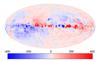Fig. 1 All-sky map, in Aitoff projection, of the observational Galactic Faraday depth, FDobs, as reconstructed by Oppermann et al. (2015). The map is in Galactic coordinates (ℓ,b), centered on the Galactic center (ℓ = 0°,b = 0°), and with longitude ℓ increasing to the left and latitude b increasing upward. Red [blue] regions have positive [negative] FDobs, corresponding to a magnetic field pointing on average toward [away from] the observer. The color intensity scales linearly with the absolute value of FDobs up to | FDobs | = 400 rad m-2 and saturates beyond this value.

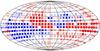Fig. 2 All-sky map, in Aitoff projection, showing the disposition of the 428 bins covering the celestial sphere, together with their average observational Galactic Faraday depth, before subtraction of the contribution from Wolleben et al.’s (2010) magnetized bubble. Positive [negative] values are plotted with red circles [blue squares], following the same color intensity scale as in Fig. 1. The coordinate system is also the same as in Fig. 1.

Faraday rotation is the rotation of the polarization direction of a linearly-polarized radio wave that passes through a magneto-ionic medium. The polarization angle θ rotates by the angle Δθ = RM λ², where λ is the observing wavelength and RM is the rotation measure given by$\mathrm{RM}\mathrm{=}\mathrm{(}\mathrm{0.81}\mathrm{rad}{\mathrm{m}}^{-2}\mathrm{)}{\mathrm{\int }}_{\mathrm{0}}^{\mathit{L}}{\mathit{n}}_{\mathrm{e}}{\mathit{B}}_{\mathrm{\parallel }}\mathrm{d}\mathit{s,}$(1)with n_e the free-electron density in cm^-3, B_∥ the line-of-sight component of the magnetic field in μG (positive [negative] for a magnetic field pointing toward [away from] the observer) and L the path length from the observer to the source measured in pc ². Clearly, RM is a purely observational quantity, which can be defined only for a linearly-polarized radio source located behind the Faraday-rotating medium.

More generally, one may use the concept of Faraday depth (Burn 1966; Brentjens & de Bruyn 2005),$\mathrm{FD}\mathrm{\left(}\mathit{d}\mathrm{\right)}\mathrm{=}\mathrm{(}\mathrm{0.81}\mathrm{rad}{\mathrm{m}}^{-2}\mathrm{)}{\mathrm{\int }}_{\mathrm{0}}^{\mathit{d}}{\mathit{n}}_{\mathrm{e}}{\mathit{B}}_{\mathrm{\parallel }}\mathrm{d}\mathit{s,}$(2)a truly physical quantity, which has the same formal expression as RM but can be defined at any point of the ISM, independent of any background source. FD simply corresponds to the line-of-sight depth of the considered point, d, measured in terms of Faraday rotation. Here, we are only interested in the FD of the Galaxy, in which case d represents the distance from the observer to the outer surface of the Galaxy along the considered line of sight.

As an observational reference for our modeling work, we adopt the all-sky map of the Galactic FD reconstructed by Oppermann et al. (2015), denoting the observational Galactic FD by FD_obs (see Fig. 1). To create their map, Oppermann et al. compiled the existing catalogs of extragalactic RMs, for a total of 41 632 data points (37 543 of which are from the NVSS catalog of Taylor et al. (2009), which covers fairly homogeneously the sky at declination δ ≥ −40°), and they employed a sophisticated signal reconstruction algorithm that takes spatial correlations into account.

The all-sky map of FD_obs in Fig. 1, like previous all-sky RM maps, shows some coherent structure on large scales. This large-scale structure in the RM sky has often been assumed to reflect, at least to some extent, the large-scale organization of the Galactic magnetic field (e.g., Simard-Normandin & Kronberg 1980; Han et al. 1997; Taylor et al. 2009). In reality, however, nearby small-scale perturbations in the magneto-ionic ISM can also leave a large-scale imprint in the RM sky (see Frick et al. 2001; Mitra et al. 2003; Wolleben et al. 2010; Mao et al. 2010; Stil et al. 2011; Sun et al. 2015, and references therein). The most prominent such perturbation identified to date is the nearby magnetized bubble uncovered by Wolleben et al. (2010) through RM synthesis (a.k.a. Faraday tomography) on polarization data from the Global Magneto-Ionic Medium Survey (GMIMS). This bubble, estimated to lie at distances around ~ 150 pc, is centered at (ℓ ≃ + 10°,b ≃ + 25°) and extends over Δℓ ≃ 70° in longitude and Δb ≃ 40° in latitude, thereby covering ≃ 5% of the sky.

Another potential source of strong contamination in the RM sky is the North Polar Spur (NPS), which extends from the Galactic plane at ℓ ≈ + 20° nearly all the way up to the north Galactic pole. However, Sun et al. (2015) showed, through Faraday tomography, that the actual Faraday thickness (ΔFD) of the NPS is most likely close to zero. They also showed that the ΔFD of the Galactic ISM behind the NPS cannot account for the entire Galactic FD toward the section of the NPS around b ≃ 30°. From this they concluded that if the NPS is local (such that the ΔFD of the ISM in front of the NPS is very small), the Galactic FD must be dominated by the ΔFD of Wolleben et al.’s (2010) magnetized bubble, which must then be larger than estimated by Wolleben et al. Clearly, the argument can be taken the other way around: if the ΔFD of the magnetized bubble is as estimated by Wolleben et al. (an assumption we will make here), the Galactic FD must have a large contribution from the ISM in front of the NPS, which implies that the section of the NPS around b ≃ 30° is not local. This last conclusion is consistent with the results of several recent studies, which systematically place the lower part of the NPS beyond a few 100 pc – more specifically: beyond the polarization horizon at 2.3 GHz, ~ (2−3) kpc, for b ≲ 4° (from Faraday depolarization; Sun et al. 2014), behind the Aquila Rift, at a distance ≳ 1 kpc, for b ≲ (15°−20°) (from X-ray absorption; Sofue 2015), and beyond the cloud complex distributed between 300 pc and ~ 600 pc and probably much farther away (again from X-ray absorption; Lallement et al. 2016).

Since the focus of our paper is on the large-scale magnetic field, we will subtract from the FD_obs map of Fig. 1 the estimated contribution from Wolleben et al.’s (2010) magnetized bubble³. We will then proceed on the assumption that the resulting FD_obs map can be relied on to constrain the large-scale magnetic field structure. As it turns out, the removal of Wolleben et al.’s bubble will systematically lead to an improvement in the quality of the fits.

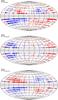Fig. 3 All-sky maps, in Aitoff projection, showing the disposition of the 356 bins with latitude | b | ≥ 10°, which are retained for the fitting procedure, together with their average observational Galactic Faraday depth, ${\overline{\mathrm{FD}}}_{\mathrm{obs}}$, after subtraction of the contribution from Wolleben et al.’s (2010) magnetized bubble (top panel). Also shown is the decomposition of ${\overline{\mathrm{FD}}}_{\mathrm{obs}}$ into a symmetric part, ${\overline{\mathrm{FD}}}_{\mathrm{obs}\mathit{,}\mathrm{S}}$ (middle panel), and an antisymmetric part, ${\overline{\mathrm{FD}}}_{\mathrm{obs}\mathit{,}\mathrm{A}}$ (bottom panel). The coordinate system and the color code are the same as in Figs. 1 and 2. The grey band along the Galactic plane masks out the 72 bins with |b| < 10°, which are excluded from the fitting.

For convenience, we bin the FD_obs data and average them within the different bins, both before (Fig. 2) and after (Fig. 3) removal of Wolleben et al.’s (2010) bubble. Following a binning procedure similar to that proposed by Pshirkov et al. (2011), we divide the sky area into 18 longitudinal bands with latitudinal width Δb = 10°, and we divide every longitudinal band into a number of bins chosen such that each of the two lowest-latitude bands contains 36 bins with longitudinal width Δℓ = 10° and all the bins have roughly the same area ≃ (10°)². This leads to a total of 428 bins. For each of these bins, we compute the average FD_obs before removal of Wolleben et al.’s bubble, and we plot it in Fig. 2, with a red circle or a blue square according to whether it is positive or negative. In both cases, the color intensity increases with the absolute value of the average FD_obs.

We then repeat the binning and averaging steps after removal of Wolleben et al.’s bubble, and for visual purposes, we wash out the obviously anomalous bin at (ℓ ≃ 0°−10°,b = 20°−30°). The underlying RM anomaly can be identified as the H ii region Sh 2-27 around ζ Oph (Harvey-Smith et al. 2011). Our exact treatment of the anomalous bin is of little importance, because its weight in the fitting procedure will be drastically reduced through an artificial tenfold increase of its estimated uncertainty, σ_i, in the expression of χ² (Eq. (39)). In practice, we just blend the anomalous bin into the background by replacing its average FD_obs with that of the super-bin enclosing its 8 direct neighbors. The bin-averaged FD_obs after removal of Wolleben et al.’s bubble and blending of the anomalous bin is denoted by ${\overline{\mathrm{FD}}}_{\mathrm{obs}}$.

Finally, since we are primarily interested in the magnetic field in the Galactic halo, we exclude the 72 bins with | b | < 10°, which leaves us with a total of 356 bins. The ${\overline{\mathrm{FD}}}_{\mathrm{obs}}$ of each of these bins is plotted in the top panel of Fig. 3, again with a red circle if ${\overline{\mathrm{FD}}}_{\mathrm{obs}}\mathit{>}\mathrm{0}$ and a blue square if ${\overline{\mathrm{FD}}}_{\mathrm{obs}}\mathit{<}\mathrm{0}$. The ${\overline{\mathrm{FD}}}_{\mathrm{obs}}$ map thus obtained provides the observational reference against which we will test our large-scale magnetic field models in Sect. 4.

2.2. General trends

A few trends emerge from the observational map of the average FD_obs in Fig. 2:

• 1.

  a rough antisymmetry with respect to the prime(ℓ = 0°) meridian;

• 2.

  a rough antisymmetry with respect to the midplane in the inner Galactic quadrants away from the plane (|ℓ| < 90° and | b | ≳ 10°);

• 3.

  a rough symmetry with respect to the midplane in the inner quadrants close to the plane (| ℓ | < 90° and | b | ≲ 10°) and in the outer quadrants (|ℓ| > 90°).

These three trends appear to persist after removal of Wolleben et al.’s (2010) bubble (see top panel of Fig. 3, for | b | ≥ 10°). We will naturally try to reproduce them with our magnetic field models, but before getting to the models, a few comments are in order.

First, the rough symmetry with respect to the midplane at | b | ≲ 10° and all ℓ suggests that the disk magnetic field is symmetric (or quadrupolar)⁴, as already pointed out by many authors (e.g., Rand & Lyne 1994; Frick et al. 2001).

Second, the rough antisymmetry [symmetry] with respect to the midplane at | b | ≳ 10° and | ℓ | < 90° [| ℓ | > 90°] suggests one of the two following possibilities: either the halo magnetic field is antisymmetric in the inner Galaxy and symmetric in the outer Galaxy, or the halo magnetic field is everywhere antisymmetric, but only toward the inner Galaxy does its contribution to the Galactic FD at | b | ≳ 10° exceed the contribution from the disk magnetic field. The first possibility is probably not very realistic (although it cannot be completely ruled out): while the disk and halo fields could possibly have different vertical parities (see, e.g., Moss & Sokoloff 2008; Moss et al. 2010), it seems likely that each field has by now evolved toward a single parity. The second possibility may sound a little counter-intuitive at first, but one has to remember that the halo field contribution to the Galactic FD is weighted by a lower free-electron density than the disk field contribution (especially toward the outer Galaxy); moreover, the halo field can very well be confined inside a smaller radius than the disk field. Such is the case in the double-torus picture originally sketched by Han (2002) and later modeled by Prouza & Šmída (2003), Sun et al. (2008), Jansson & Farrar (2012a): in these three models, the toroidal field of the halo falls off exponentially with r at large radii, i.e., much faster than the disk field, which falls off approximately as (1 /r).

Third, the rough antisymmetry with respect to the prime meridian (east-west antisymmetry) can a priori be explained by an axisymmetric, predominantly azimuthal magnetic field. However, the situation is a little more subtle.

• For the disk, RM studies (mainly of Galactic pulsars, and also ofextragalactic point sources) converge to show that the magneticfield is indeed predominantly azimuthal, though not with thesame sign everywhere throughout the disk, i.e., the field mustreverse direction with Galactic radius (e.g., Rand& Lyne 1994; Hanet al. 1999, 2006; Brownet al. 2007). The exactnumber and the radial locations of these reversals arestill a matter of debate, which we do not whish to en-ter. Here, we are content to note that field reversals nat-urally arise in a bisymmetric (azimuthal modulation∝ cosmϕ, with m = 1) or higher-order (m> 1) configuration, but can also be produced in the axisymmetric case (Ferrière & Schmitt 2000).

• For the halo, most existing models have settled on a purely azimuthal, and hence axisymmetric, magnetic field. Here, we inquire into the other possibilities. Let us first ask whether a purely poloidal (possibly, but not necessarily, X-shape) magnetic field would be a viable alternative. Clearly, a purely poloidal field that is axisymmetric automatically leads to an FD pattern with east-west symmetry, inconsistent with the observed FD distribution. In contrast, a purely poloidal field that is bisymmetric can lead to a variety of FD patterns, depending on the azimuthal angle of maximum amplitude: if the maximum amplitude occurs in the azimuthal plane parallel to the plane of the sky (ϕ = ± 90°) [in the azimuthal plane through the Sun (ϕ = 0°)], the FD pattern has east-west antisymmetry [symmetry], in agreement [disagreement] with the observed FD distribution. Hence, a purely poloidal magnetic field can possibly match the FD data, provided it is bisymmetric (or higher-order) and favorably oriented. Let us now turn to the more general and more realistic situation where the magnetic field has both azimuthal and poloidal components, as required by dynamo theory. If this general field is axisymmetric, the observed east-west antisymmetry in FD implies that it must be mainly azimuthal. In contrast, if the general field is bisymmetric, it could in principle cover a broad range of orientation, from mostly azimuthal to mostly poloidal. What happens here is that, in the presence of an azimuthal field component, the azimuthal modulation, which is presumably carried along field lines, crosses azimuthal planes. The resulting FD pattern becomes more difficult to predict: it may become more complex and fluctuating than in the axisymmetric case, and large-scale longitudinal trends may be partly washed out, but a priori the predominance of neither the azimuthal nor the poloidal field component can be ruled out. To sum up, the halo magnetic field could either be axisymmetric and mainly azimuthal or bisymmetric (or higher-order) with no clear constraint on its azimuthal-versus-poloidal status.

3. Magnetic field models

3.1. Magnetic fields in galactic halos

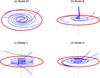Fig. 4 Small set of field lines for each of our four models of spiraling, possibly X-shape magnetic fields in galactic halos, as seen from an oblique angle. The shapes of field lines for the three halo-field models A1, B, and D are also representative of our three disk-field models Ad1, Bd, and Dd. All the plotted field lines lie on the same winding surface (Eq. (26) with ϕ∞ = 0° and gϕ(r,z) given by Eq. (23) with p0 = −9°, Hp = 1.5 kpc, and Lp = 45 kpc), and their footpoints, (r1,ϕ1,z1), on the relevant reference surface (r = r1 in models A1 and B, and z = z1 in models C and D) are given by: a)(3 kpc,172°,0.5 kpc) and (3 kpc,357°,2 kpc) in model A1 (with a = 0.05 kpc-2); b)(3 kpc,326°,1 kpc), (3 kpc,357°,2 kpc), and (3 kpc,198°,3 kpc) in model B (with n = 2); c)(2.5 kpc,336°,0) and (7.5 kpc,318°,0) in model C (with a = 0.01 kpc-2); and d)(2.5 kpc,168°,1.5 kpc), (5 kpc,47°,1.5 kpc), and (7.5 kpc,339°,1.5 kpc) in model D (with n = 0.5). The galactic plane is represented by the red, solid circle of radius 15 kpc, and the rotation axis by the vertical, black, dot-dashed line.

In Paper I, we derived four different models of spiraling, possibly X-shape magnetic fields in galactic halos, which can be applied to the halo of our own Galaxy. Each of these models was initially defined by the shape of its field lines together with the distribution of the magnetic flux density on a given reference surface. Using the Euler formalism (e.g., Northrop 1963; Stern 1966), we were able to work out the corresponding analytical expression of the magnetic field vector, B = (B_r,B_ϕ,B_z), as a function of Galactocentric cylindrical coordinates, (r,ϕ,z). The main characteristics of the four halo-field models are summarized below, and a few representative field lines are plotted in Fig. 4.

In models A and B, we introduced a fixed reference radius, r₁, and we labeled field lines by the height, z₁, and the azimuthal angle, ϕ₁, at which they cross the centered vertical cylinder of radius r₁. In models C and D, we introduced a fixed reference height, z₁ (more exactly, one reference height, z₁ = 0, in model C where all field lines cross the galactic midplane, and two reference heights, z₁ = ± | z₁ |, in model D where field lines do not cross the midplane), and we labeled field lines by the radius, r₁, and the azimuthal angle, ϕ₁, at which they cross the horizontal plane (or one of the two horizontal planes) of height z₁. Thus, in all models, the point (r₁,ϕ₁,z₁) of a given field line can be regarded as its footpoint on the reference surface (vertical cylinder of radius r₁ in models A and B and horizontal plane(s) of height z₁ in models C and D).

3.1.1. Poloidal field

The four models are distinguished by the shape of field lines associated with the poloidal field (hereafter referred to as the poloidal field lines), and hence by the expressions of the radial and vertical field components.

In model A, the shape of poloidal field lines is described by the quadratic function 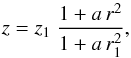$\mathit{z}\mathrm{=}{\mathit{z}}_{\mathrm{1}}\frac{\mathrm{1}\mathrm{+}\mathit{a}\hspace{0.17em}{\mathit{r}}^{\mathrm{2}}}{\mathrm{1}\mathrm{+}\mathit{a}\hspace{0.17em}{\mathit{r}}_{\mathrm{1}}^{\mathrm{2}}}\mathit{,}$(3)where a is a strictly positive free parameter governing the opening of field lines away from the z-axis, r₁ is the prescribed reference radius, and z₁ is the vertical label of the considered field line. Conversely, the vertical label of the field line passing through (r,ϕ,z) is given by 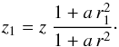${\mathit{z}}_{\mathrm{1}}\mathrm{=}\mathit{z}\frac{\mathrm{1}\mathrm{+}\mathit{a}\hspace{0.17em}{\mathit{r}}_{\mathrm{1}}^{\mathrm{2}}}{\mathrm{1}\mathrm{+}\mathit{a}\hspace{0.17em}{\mathit{r}}^{\mathrm{2}}}\mathrm{·}$(4)It then follows (see Paper I for the detailed derivation) that the poloidal field components can be written as$\begin{array}{ccc}{\mathit{B}}_{\mathit{r}}& \mathrm{=}& \\ {\mathit{B}}_{\mathit{z}}& \mathrm{=}& \end{array}$with, for instance, B_r(r₁,ϕ₁,z₁) obeying Eq. (11).

In model B, the corresponding equations read$\mathit{z}\mathrm{=}\frac{\mathrm{1}}{\mathit{n}\mathrm{+}\mathrm{1}}{\mathit{z}}_{\mathrm{1}}\left[{\left(\frac{\mathit{r}}{{\mathit{r}}_{\mathrm{1}}}\right)}^{\mathrm{-}\mathit{n}}\mathrm{+}\mathit{n}\hspace{0.17em}\frac{\mathit{r}}{{\mathit{r}}_{\mathrm{1}}}\right]\mathit{,}$(7)with n a power-law index satisfying the constraint n ≥ 1,${\mathit{z}}_{\mathrm{1}}\mathrm{=}\mathrm{(}\mathit{n}\mathrm{+}\mathrm{1}\mathrm{)}\mathit{z}{\left[{\left(\frac{\mathit{r}}{{\mathit{r}}_{\mathrm{1}}}\right)}^{\mathrm{-}\mathit{n}}\mathrm{+}\mathit{n}\hspace{0.17em}\frac{\mathit{r}}{{\mathit{r}}_{\mathrm{1}}}\right]}^{-1}\mathit{,}$(8)and$\begin{array}{ccc}{\mathit{B}}_{\mathit{r}}& \mathrm{=}& \\ {\mathit{B}}_{\mathit{z}}& \mathrm{=}& \end{array}$

In both models A and B, the radial field component on the vertical cylinder of radius r₁ is chosen to have a linear-exponential variation with z₁ and a sinusoidal variation with ϕ₁:$\begin{array}{ccc}{\mathit{B}}_{\mathit{r}}\mathrm{\left(}{\mathit{r}}_{\mathrm{1}}\mathit{,}{\mathit{\varphi }}_{\mathrm{1}}\mathit{,}{\mathit{z}}_{\mathrm{1}}\mathrm{\right)}& \mathrm{=}& {\mathit{B}}_{\mathrm{1}}{\mathit{f}}_{\mathrm{sym}}\left[\frac{\mathrm{\left|}{\mathit{z}}_{\mathrm{1}}\mathrm{\right|}}{\mathit{H}}\exp \left(\mathrm{-}\frac{\mathrm{\left|}{\mathit{z}}_{\mathrm{1}}\mathrm{\right|}\mathrm{-}\mathit{H}}{\mathit{H}}\right)\right]\\ & \mathrm{\times }& \end{array}$(11)where B₁ is the normalization field strength, f_sym is a factor setting the vertical parity of the magnetic field (f_sym = 1 for symmetric fields and f_sym = sign z₁ for antisymmetric fields; see footnote 4), H is the exponential scale height, m is the azimuthal wavenumber, g_ϕ is the shifted winding function defined by Eq. (23), and ϕ_⋆ is the orientation angle of the azimuthal pattern. The term g_ϕ(r₁,z₁), which will be discussed in more detail in Sect. 3.1.2, ensures that the phase of the sinusoidal modulation remains constant on the winding surfaces defined by Eq. (26) (see comment following Eq. (26)).

Models C and D are the direct counterparts of models A and B, respectively, with the roles of the coordinates r and z inverted in the equations of field lines.

In model C, the reference height is set to z₁ = 0, and the shape of poloidal field lines is described by the quadratic function$\mathit{r}\mathrm{=}{\mathit{r}}_{\mathrm{1}}\mathrm{(}\mathrm{1}\mathrm{+}\mathit{a}\hspace{0.17em}{\mathit{z}}^{\mathrm{2}}\mathrm{)}\mathit{,}$(12)with a a strictly positive free parameter governing the opening of field lines away from the r-axis and r₁ the radial label of the considered field line. Conversely, the radial label of the field line passing through (r,ϕ,z) is given by${\mathit{r}}_{\mathrm{1}}\mathrm{=}\frac{\mathit{r}}{\mathrm{1}\mathrm{+}\mathit{a}\hspace{0.17em}{\mathit{z}}^{\mathrm{2}}}\mathrm{·}$(13)The poloidal field components can then be written as$\begin{array}{ccc}{\mathit{B}}_{\mathit{r}}& \mathrm{=}& \\ {\mathit{B}}_{\mathit{z}}& \mathrm{=}& \end{array}$with, for instance, B_z(r₁,ϕ₁,z₁) obeying Eq. (20).

In model D, where every field line remains confined to one side of the galactic midplane, a reference height, z₁ = | z₁ | sign z, is prescribed on each side of the midplane, such that the ratio (z/z₁) is always positive. We then have $\mathit{r}\mathrm{=}\frac{\mathrm{1}}{\mathit{n}\mathrm{+}\mathrm{1}}{\mathit{r}}_{\mathrm{1}}\left[{\left(\frac{\mathit{z}}{{\mathit{z}}_{\mathrm{1}}}\right)}^{\mathrm{-}\mathit{n}}\mathrm{+}\mathit{n}\hspace{0.17em}\frac{\mathit{z}}{{\mathit{z}}_{\mathrm{1}}}\right]\mathit{,}$(16)with n ≥ 0.5, ${\mathit{r}}_{\mathrm{1}}\mathrm{=}\mathrm{(}\mathit{n}\mathrm{+}\mathrm{1}\mathrm{)}\mathit{r}{\left[{\left(\frac{\mathit{z}}{{\mathit{z}}_{\mathrm{1}}}\right)}^{\mathrm{-}\mathit{n}}\mathrm{+}\mathit{n}\hspace{0.17em}\frac{\mathit{z}}{{\mathit{z}}_{\mathrm{1}}}\right]}^{-1}\mathit{,}$(17)and $\begin{array}{ccc}{\mathit{B}}_{\mathit{r}}& \mathrm{=}& \\ {\mathit{B}}_{\mathit{z}}& \mathrm{=}& \end{array}$

In both models C and D, the vertical field component on the horizontal plane(s) of height z₁ is chosen to have an exponential variation with r₁ and a sinusoidal variation with ϕ₁: ${\mathit{B}}_{\mathit{z}}\mathrm{\left(}{\mathit{r}}_{\mathrm{1}}\mathit{,}{\mathit{\varphi }}_{\mathrm{1}}\mathit{,}{\mathit{z}}_{\mathrm{1}}\mathrm{\right)}\mathrm{=}{\mathit{B}}_{\mathrm{1}}\mathit{f̅}\mathrm{sym}\exp \left(\mathrm{-}\frac{{\mathit{r}}_{\mathrm{1}}}{\mathit{L}}\right)\cos (\mathit{m}\hspace{0.17em}({\mathit{\varphi }}_{\mathrm{1}}\mathrm{-}{\mathit{g}}_{\mathit{\varphi }}\mathrm{\left(}{\mathit{r}}_{\mathrm{1}}\mathit{,}{\mathit{z}}_{\mathrm{1}}\mathrm{\right)}\mathrm{-}{\mathit{\varphi }}_{\mathit{\star }}))\mathit{,}$(20)with B₁ the normalization field strength, a factor setting the vertical parity of the magnetic field ( in model C, which is always antisymmetric, and in the antisymmetric version of model D, and in the symmetric version of model D; see footnote 4), L the exponential scale length, m the azimuthal wavenumber, g_ϕ the shifted winding function (Eq. (23)), and ϕ_⋆ the orientation angle of the azimuthal pattern.

3.1.2. Azimuthal field

In all four models, field lines are assumed to spiral up or down according to the equation $\mathit{\varphi }\mathrm{=}{\mathit{\varphi }}_{\mathrm{1}}\mathrm{+}{\mathit{f}}_{\mathit{\varphi }}\mathrm{\left(}\mathit{r,z}\mathrm{\right)}\mathit{,}$(21)where f_ϕ(r,z) is a winding function starting from the field line’s footpoint on the reference surface and, therefore, satisfying f_ϕ(r₁,z₁) = 0. If we consider that field lines are somehow anchored in the external intergalactic medium⁵, it proves more convenient to shift the starting point of the winding function to infinity. This can be done by letting ${\mathit{f}}_{\mathit{\varphi }}\mathrm{\left(}\mathit{r,z}\mathrm{\right)}\mathrm{=}{\mathit{g}}_{\mathit{\varphi }}\mathrm{\left(}\mathit{r,z}\mathrm{\right)}\mathrm{-}{\mathit{g}}_{\mathit{\varphi }}\mathrm{\left(}{\mathit{r}}_{\mathrm{1}}\mathit{,}{\mathit{z}}_{\mathrm{1}}\mathrm{\right)}\mathit{,}$(22)where g_ϕ(r,z) is a shifted winding function starting from the field line’s anchor point at infinity⁶ and, therefore, satisfying g_ϕ(r,z) → 0 for r → ∞ and for | z | → ∞. A reasonably simple choice for the shifted winding function is ${\mathit{g}}_{\mathit{\varphi }}\mathrm{\left(}\mathit{r,z}\mathrm{\right)}\mathrm{=}\cot {\mathit{p}}_{\mathrm{0}}\frac{\ln \left[\mathrm{1}\mathrm{-}\exp \left(\mathrm{-}\frac{\mathit{r}}{{\mathit{L}}_{\mathit{p}}}\right)\right]}{\mathrm{1}\mathrm{+}{\left(\frac{\mathrm{\left|}\mathit{z}\mathrm{\right|}}{{\mathit{H}}_{\mathit{p}}}\right)}^{\mathrm{2}}}\mathit{,}$(23)with p₀ the pitch angle (i.e., the angle between the horizontal projection of a field line and the local azimuthal direction) at the origin ((r,z) → 0), H_p the scale height, and L_p the exponential scale length. With this choice, g_ϕ(r,z) defines, in horizontal planes (z = const.), spirals that are logarithmic (constant pitch angle) at small r and become increasingly loose (increasing pitch angle) at large r. The spirals also loosen up with increasing | z |.

Combining Eqs. (21) and (22), we can rewrite the equation describing the spiraling of field lines in the form $\mathit{\varphi }\mathrm{=}{\mathit{g}}_{\mathit{\varphi }}\mathrm{\left(}\mathit{r,z}\mathrm{\right)}\mathrm{+}\mathrm{[}{\mathit{\varphi }}_{\mathrm{1}}\mathrm{-}{\mathit{g}}_{\mathit{\varphi }}\mathrm{(}{\mathit{r}}_{\mathrm{1}}\mathit{,}{\mathit{z}}_{\mathrm{1}}{\mathrm{\left)}}^{\mathrm{\right]}}\mathit{,}$(24)with ${}^{\mathrm{[}}\mathit{\varphi }_{\mathrm{1}}\mathrm{-}{\mathit{g}}_{\mathit{\varphi }}\mathrm{(}{\mathit{r}}_{\mathrm{1}}\mathit{,}{\mathit{z}}_{\mathrm{1}}{\mathrm{\left)}}^{\mathrm{\right]}}$ constant along field lines. Conversely, the field line passing through (r,ϕ,z) can be traced back to the azimuthal label ${\mathit{\varphi }}_{\mathrm{1}}\mathrm{=}\mathit{\varphi }\mathrm{-}{\mathit{g}}_{\mathit{\varphi }}\mathrm{\left(}\mathit{r,z}\mathrm{\right)}\mathrm{+}{\mathit{g}}_{\mathit{\varphi }}\mathrm{\left(}{\mathit{r}}_{\mathrm{1}}\mathit{,}{\mathit{z}}_{\mathrm{1}}\mathrm{\right)}\mathit{,}$(25)where r₁ and z₁ either have prescribed values or are given functions of (r,z) (see Eqs. (4), (8), (13), and (17) in Sect. 3.1.1). It then follows from Eqs. (11) and (20) that the sinusoidal modulation of the magnetic field goes as cos(m (ϕ−g_ϕ(r,z)−ϕ_⋆)).

If we now consider the anchor point at infinity⁶ of the field line passing through (r,ϕ,z), denote its azimuthal angle by ϕ_∞, and recall that g_ϕ(r,z) → 0 for r, | z | → ∞, we find that the spiraling of field line can also be described by $\mathit{\varphi }\mathrm{=}{\mathit{g}}_{\mathit{\varphi }}\mathrm{\left(}\mathit{r,z}\mathrm{\right)}\mathrm{+}{\mathit{\varphi }}_{\mathrm{\infty }}\mathit{.}$(26)Equation (26) defines a so-called winding surface, formed by all the field lines with the same azimuthal angle at infinity, ϕ_∞, and thus the same phase in the sinusoidal modulation, ϕ_∞−ϕ_⋆. The crest of the modulation occurs at phase ϕ_∞−ϕ_⋆ = 0°, i.e., at ϕ_∞ = ϕ_⋆, which means that the free parameter ϕ_⋆ can be interpreted as the azimuthal angle at infinity of the crest surface.

Since the magnetic field is by definition tangent to field lines, Eq. (24) implies that its azimuthal component is related to its radial and vertical components through 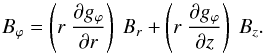${\mathit{B}}_{\mathit{\varphi }}\mathrm{=}\left(\mathit{r}\frac{\mathit{\partial }{\mathit{g}}_{\mathit{\varphi }}}{\mathit{\partial r}}\right){\mathit{B}}_{\mathit{r}}\mathrm{+}\left(\mathit{r}\frac{\mathit{\partial }{\mathit{g}}_{\mathit{\varphi }}}{\mathit{\partial z}}\right){\mathit{B}}_{\mathit{z}}\mathit{.}$(27)Roughly speaking, the two terms on the right-hand side of Eq. (27) represent the azimuthal field generated through shearing of radial and vertical fields by radial and vertical gradients in the galactic rotation rate, respectively. With the choice of Eq. (23), Eq. (27) becomes $\begin{array}{ccc}{\mathit{B}}_{\mathit{\varphi }}& \mathrm{=}& \cot {\mathit{p}}_{\mathrm{0}}\frac{\mathrm{1}}{\mathrm{1}\mathrm{+}{\left(\frac{\mathrm{\left|}\mathit{z}\mathrm{\right|}}{{\mathit{H}}_{\mathit{p}}}\right)}^{\mathrm{2}}}\frac{\frac{\mathit{r}}{{\mathit{L}}_{\mathit{p}}}\exp \left(\mathrm{-}\frac{\mathit{r}}{{\mathit{L}}_{\mathit{p}}}\right)}{\mathrm{1}\mathrm{-}\exp \left(\mathrm{-}\frac{\mathit{r}}{{\mathit{L}}_{\mathit{p}}}\right)}{\mathit{B}}_{\mathit{r}}\\ & \mathrm{-}& \end{array}$(28)It is easily seen that the factor of B_r has the same sign as cotp₀ (usually negative) everywhere, while the factor of B_z has the same sign as cotp₀ above the midplane (z> 0) and the opposite sign below the midplane (z< 0).

3.1.3. Total field

To sum up, the poloidal field is described by Eqs. (5)–(6) in model A and Eqs. (9)–(10) in model B, with B_r(r₁,ϕ₁,z₁) given by Eq. (11), and by Eqs. (14)–(15) in model C and Eqs. (18)–(19) in model D, with B_z(r₁,ϕ₁,z₁) given by Eq. (20). The azimuthal field is described by Eq. (28) in all models. Together, the above equations link the magnetic field at an arbitrary point (r,ϕ,z) to the normal field component at the footpoint (r₁,ϕ₁,z₁) on the reference surface of the field line passing through (r,ϕ,z). The footpoint, in turn, is determined by the reference coordinate (r₁ in models A and B, and z₁ in models C and D, with z₁ = 0 in model C and z₁ = ± | z₁ | in model D), the poloidal label of the field line (z₁ given by Eq. (4) in model A and Eq. (8) in model B, and r₁ given by Eq. (13) in model C and Eq. (17) in model D), and its azimuthal label (ϕ₁ given by Eq. (25) in all models).

3.1.4. Regularization of model A

An important remark should be made regarding model A. Eq. (5) together with Eq. (4) imply that B_r → ∞ for r → 0, which reflects the fact that all field lines, from all azimuthal planes, converge to the z-axis. The problem does not arise in model B, as shown by Eq. (9) together with Eq. (8), because all field lines are deflected vertically before reaching the z-axis (see Fig. 4b). The singularity in model A is inescapable in the axisymmetric case (m = 0 in Eq. (11)), where B_r has the same sign all around the z-axis, so that, at every height, a non-zero magnetic flux reaches the z-axis. However, the singularity can be removed in non-axisymmetric (m ≥ 1) configurations, where B_r changes sign sinusoidally around the z-axis, so that, at every height, no net magnetic flux actually reaches the z-axis. It is then conceivable to detach field lines from the z-axis, spread them apart inside a centered vertical cylinder, whose radius can be chosen to be r₁ (remember that r₁ is still a free parameter at this stage), and connect up two by two field lines with the same z₁, opposite ϕ₁ (with respect to a node of the sinusoidal modulation in Eq. (11)), and hence opposite B_r, such as to ensure conservation of the magnetic flux as well as continutity in its sign.

For instance, in the bisymmetric (m = 1) case, field lines with the same z₁ and opposite ϕ₁ (with respect to g_ϕ(r₁,z₁) + ϕ_⋆ ± π/ 2) can be connected up inside the vertical cylinder of radius r₁ through straight-line segments parallel to the direction ϕ₁ = g_ϕ(r₁,z₁) + ϕ_⋆. In this case, magnetic flux conservation (or continuity of B_r) across the surface of the cylinder gives for the magnetic field at an arbitrary point (r,ϕ,z) inside the cylinder: $\begin{array}{ccc}{B}& \mathrm{=}& {\mathit{B}}_{\mathit{r}}({\mathit{r}}_{\mathrm{1}}\mathit{,}{\mathit{g}}_{\mathit{\varphi }}\mathrm{\left(}{\mathit{r}}_{\mathrm{1}}\mathit{,}{\mathit{z}}_{\mathrm{1}}\mathrm{\right)}\mathrm{+}{\mathit{\varphi }}_{\mathit{\star }}\mathit{,}{\mathit{z}}_{\mathrm{1}})\mathit{ê}\mathit{\star }\mathrm{\left(}{\mathit{z}}_{\mathrm{1}}\mathrm{\right)}\\ & \mathrm{=}& \end{array}$(29)with z₁ = z, ê_⋆(z₁) the unit vector in the direction ϕ₁ = g_ϕ(r₁,z₁) + ϕ_⋆, and the other symbols having the same meaning as in Eq. (11).

In the following, the regularized bisymmetric version of model A is referred to as model A1, where the number 1 indicates the value of the azimuthal wavenumber.

3.2. Magnetic fields in galactic disks

We now present three different models of spiraling, mainly horizontal magnetic fields in galactic disks, which can be applied to the disk of our own Galaxy. These models are directly inspired from the three models for magnetic fields in galactic halos that have nearly horizontal field lines at low | z |, namely, models A1, B, and D in Sect. 3.1, and they are named models Ad1, Bd, and Dd, respectively. Models Bd and Dd are directly taken up from Paper I, with a minor amendment in model Dd (see below), while model Ad1 is a new addition.

Model Ad1 has nearly the same descriptive equations as model A1. Outside the reference radius, r₁, the shape of field lines is described by Eq. (3), with the parameter a assuming a much smaller value than for halo fields, and by Eq. (24); the vertical and azimuthal labels of the field line passing through (r,ϕ,z) are given by Eqs. (4) and (25); and the three magnetic field components obey Eqs. (5), (6), and (28), with 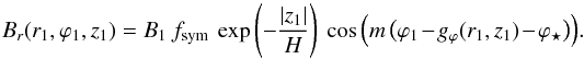${\mathit{B}}_{\mathit{r}}\mathrm{\left(}{\mathit{r}}_{\mathrm{1}}\mathit{,}{\mathit{\varphi }}_{\mathrm{1}}\mathit{,}{\mathit{z}}_{\mathrm{1}}\mathrm{\right)}\mathrm{=}{\mathit{B}}_{\mathrm{1}}{\mathit{f}}_{\mathrm{sym}}\exp \left(\mathrm{-}\frac{\mathrm{\left|}{\mathit{z}}_{\mathrm{1}}\mathrm{\right|}}{\mathit{H}}\right)\cos (\mathit{m}\hspace{0.17em}({\mathit{\varphi }}_{\mathrm{1}}\mathrm{-}{\mathit{g}}_{\mathit{\varphi }}\mathrm{\left(}{\mathit{r}}_{\mathrm{1}}\mathit{,}{\mathit{z}}_{\mathrm{1}}\mathrm{\right)}\mathrm{-}{\mathit{\varphi }}_{\mathit{\star }}))\mathit{.}$(30)All the symbols entering Eq. (30) have the same meaning as in Eq. (11); the difference between both equations resides in the z₁-dependence of B_r, which leads to a peak at | z₁ | = H (appropriate for halo fields) in Eq. (11) and a peak at z₁ = 0 (appropriate for disk fields) in Eq. (30). Inside r₁, field lines are straight, horizontal (z = z₁), and parallel to the unit vector ê_⋆(z₁) in the direction ϕ₁ = g_ϕ(r₁,z₁) + ϕ_⋆, and the magnetic field vector is given by Eq. (29) adjusted to Eq. (30): 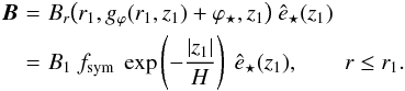$\begin{array}{ccc}{B}& \mathrm{=}& {\mathit{B}}_{\mathit{r}}({\mathit{r}}_{\mathrm{1}}\mathit{,}{\mathit{g}}_{\mathit{\varphi }}\mathrm{\left(}{\mathit{r}}_{\mathrm{1}}\mathit{,}{\mathit{z}}_{\mathrm{1}}\mathrm{\right)}\mathrm{+}{\mathit{\varphi }}_{\mathit{\star }}\mathit{,}{\mathit{z}}_{\mathrm{1}})\mathit{ê}\mathit{\star }\mathrm{\left(}{\mathit{z}}_{\mathrm{1}}\mathrm{\right)}\\ & \mathrm{=}& \end{array}$(31)

Model Bd is a slight variant of model B. Given a reference radius, r₁, the shape of field lines is described by $\mathit{z}\mathrm{=}\frac{\mathrm{1}}{\mathrm{2}\mathit{n}\mathrm{+}\mathrm{1}}{\mathit{z}}_{\mathrm{1}}\left[{\left(\frac{\mathit{r}}{{\mathit{r}}_{\mathrm{1}}}\right)}^{\mathrm{-}\mathit{n}}\mathrm{+}\mathrm{2}\mathit{n}\hspace{0.17em}\sqrt{\frac{\mathit{r}}{{\mathit{r}}_{\mathrm{1}}}}\right]\mathit{,}$(32)with n ≥ 2, and by Eq. (24); the vertical and azimuthal labels of the field line passing through (r,ϕ,z) are given by ${\mathit{z}}_{\mathrm{1}}\mathrm{=}\mathrm{(}\mathrm{2}\mathit{n}\mathrm{+}\mathrm{1}\mathrm{)}\mathit{z}{\left[{\left(\frac{\mathit{r}}{{\mathit{r}}_{\mathrm{1}}}\right)}^{\mathrm{-}\mathit{n}}\mathrm{+}\mathrm{2}\mathit{n}\hspace{0.17em}\sqrt{\frac{\mathit{r}}{{\mathit{r}}_{\mathrm{1}}}}\right]}^{-1}$(33)and by Eq. (25), respectively; and the three magnetic field components obey $\begin{array}{ccc}{\mathit{B}}_{\mathit{r}}& \mathrm{=}& \\ {\mathit{B}}_{\mathit{z}}& \mathrm{=}& \end{array}$and Eq. (28), together with Eq. (30).

Model Dd is nearly the same as model D. Given a reference height on each side of the midplane, z₁ = | z₁ | sign z, the shape of field lines is described by Eq. (16), with n = 0.5, and by Eq. (24); the radial and azimuthal labels of the field line passing through (r,ϕ,z) are given by Eqs. (17) and (25); and the three magnetic field components obey Eqs. (18), (19), and (28), with ${\mathit{B}}_{\mathit{z}}\mathrm{\left(}{\mathit{r}}_{\mathrm{1}}\mathit{,}{\mathit{\varphi }}_{\mathrm{1}}\mathit{,}{\mathit{z}}_{\mathrm{1}}\mathrm{\right)}\mathrm{=}{\mathit{B}}_{\mathrm{1}}\mathit{f̅}\mathrm{sym}\mathit{F}\mathrm{\left(}{\mathit{r}}_{\mathrm{1}}\mathrm{\right)}\cos (\mathit{m}\hspace{0.17em}({\mathit{\varphi }}_{\mathrm{1}}\mathrm{-}{\mathit{g}}_{\mathit{\varphi }}\mathrm{\left(}{\mathit{r}}_{\mathrm{1}}\mathit{,}{\mathit{z}}_{\mathrm{1}}\mathrm{\right)}\mathrm{-}{\mathit{\varphi }}_{\mathit{\star }}))$(36)and $\mathit{F}\mathrm{\left(}{\mathit{r}}_{\mathrm{1}}\mathrm{\right)}\mathrm{=}\{\begin{array}{c}\\ \mathrm{1}\mathit{,}& {\mathit{r}}_{\mathrm{1}}\mathrm{\le }\mathit{L}\\ \exp \left(\mathrm{-}\frac{{\mathit{r}}_{\mathrm{1}}\mathrm{-}\mathit{L}}{\mathit{L}}\right)\mathit{,}& {\mathit{r}}_{\mathrm{1}}\mathrm{\ge }\mathit{L}\mathit{.}\end{array}$(37)Equation (36) is the counterpart of Eq. (20), with the radial exponential cut off for r₁ ≤ L. The effect of this cutoff is to reduce the crowding of field lines along the midplane.

4. Method

4.1. Simulated Galactic Faraday depth

As explained earlier, our purpose is to study the structure of the magnetic field in the Galactic halo. We are not directly interested in the exact attributes of the disk magnetic field, but we may not ignore the disk field altogether: since all sightlines originating from the Sun pass through the disk (if only for a short distance before entering the halo), we need to have a good description of the disk field in the interstellar vicinity of the Sun.

Therefore, all our Galactic magnetic field models must include a disk field and a halo field. Moreover, in view of the general trends discussed in Sect. 2.2, we expect the disk field to be roughly symmetric and the halo field roughly antisymmetric with respect to the midplane. Alternatively, we may consider that the Galactic magnetic field is composed of a symmetric field, which dominates in the disk, and an antisymmetric field, which dominates in the halo. In other words, we may write the complete Galactic magnetic field as ${B}\mathrm{=}{{B}}_{\mathrm{S}}\mathrm{+}{{B}}_{\mathrm{A}}\mathit{,}$(38)where B_S is the symmetric field, described by one of the disk-field models (models Ad1, Bd, or Dd; see Sect. 3.2), and B_A is the antisymmetric field, described by one of the halo-field models (models A1, B, C, or D; see Sect. 3.1).

Our knowledge of the large-scale magnetic field at the Sun, B_⊙, imposes two constraints on our magnetic field models. Since the Sun is assumed to lie in the midplane (z_⊙ = 0), where B_A vanishes, these constraints apply only to B_S. From the RMs of nearby pulsars, Rand & Kulkarni (1989) derived a local field strength B_⊙ ≃ 1.6 μG, while Rand & Lyne (1994), Han & Qiao (1994) obtained B_⊙ ≃ 1.4 μG. All three studies found B_⊙ to be running clockwise about the rotation axis ((B_ϕ)_⊙> 0). Han & Qiao (1994) also derived a local pitch angle p_⊙ ≃ −8.2° (implying (B_r)_⊙< 0), close to the value p_⊙ ≃ −7.2° inferred from the polarization of nearby stars (Heiles 1996). In the following, we restrict the range of B_⊙ to [1,2] μG and the range of p_⊙ to [−15°,−4° ]. The implications of these restrictions are discussed at the end of Appendix C.1.

To calculate the Galactic FD (Eq. (2)), we also need a model for the free-electron density, n_e. Here, we adopt the NE2001 model of Cordes & Lazio (2002), with revised values for the parameters of the thick disk component. Gaensler et al. (2008) found that the scale height of the thick disk in the NE2001 model was underestimated by almost a factor of 2; they derived a new scale height of 1.83 kpc (up from 0.95 kpc) and a new midplane density of 0.014 cm^-3 (down from 0.035 cm^-3). This revision prompted several authors to adopt the NE2001 model and simply replace the parameters of the thick disk with the new values derived by Gaensler et al., while keeping all the other components unchanged (Sun & Reich 2010; Pshirkov et al. 2011; Jansson & Farrar 2012a). However, Schnitzeler (2012) showed that this simple modification entails internal inconsistencies, as the thick disk of Gaensler et al. overlaps with the local ISM and local spiral arm components of the NE2001 model. By correctly accounting for all the components of the NE2001 model, Schnitzeler (2012) updated the thick disk with a scale height of 1.31 kpc and a midplane density of 0.016 cm^-3. These are the values that we adopt for our FD calculation. For future reference, the scale length of the thick disk is ≃ 11 kpc.

For any considered magnetic field model, we can now use Eq. (2) to calculate the modeled Galactic FD, FD_mod, as a function of position in the sky. To produce a modeled FD map that is directly comparable to the observational map of ${\overline{\mathrm{FD}}}_{\mathrm{obs}}$ displayed in the top panel of Fig. 3, we divide the sky area into the same 428 bins as in the ${\overline{\mathrm{FD}}}_{\mathrm{obs}}$ map, and we only retain the same N_bin = 356 bins with | b | ≥ 10°. For each of these bins, we compute FD_mod along 20 well-separated sightlines (which is sufficient, in view of the smoothness of our large-scale field models, to reach the required accuracy), and we average the computed FD_mod to obtain ${\overline{\mathrm{FD}}}_{\mathrm{mod}}$. The resulting modeled map of ${\overline{\mathrm{FD}}}_{\mathrm{mod}}$ can then be compared to the observational map of ${\overline{\mathrm{FD}}}_{\mathrm{obs}}$.

To disentangle the impact of the different model parameters and to guide (and ultimately speed up) the global fitting process, it helps to first consider B_S and B_A separately, denoting the associated ${\overline{\mathrm{FD}}}_{\mathrm{mod}}$ by ${\overline{\mathrm{FD}}}_{\mathrm{mod}\mathit{,}\mathrm{S}}$ and ${\overline{\mathrm{FD}}}_{\mathrm{mod}\mathit{,}\mathrm{A}}$, respectively. If the slight vertical asymmetry in the free-electron density distribution (which essentially arises from the local ISM component in the NE2001 model) is ignored, ${\overline{\mathrm{FD}}}_{\mathrm{mod}\mathit{,}\mathrm{S}}$ and ${\overline{\mathrm{FD}}}_{\mathrm{mod}\mathit{,}\mathrm{A}}$ represent the symmetric and antisymmetric parts of ${\overline{\mathrm{FD}}}_{\mathrm{mod}}$. Accordingly, we will first adjust ${\overline{\mathrm{FD}}}_{\mathrm{mod}\mathit{,}\mathrm{S}}$ to ${\overline{\mathrm{FD}}}_{\mathrm{obs}\mathit{,}\mathrm{S}}$ and ${\overline{\mathrm{FD}}}_{\mathrm{mod}\mathit{,}\mathrm{A}}$ to ${\overline{\mathrm{FD}}}_{\mathrm{obs}\mathit{,}\mathrm{A}}$, where ${\overline{\mathrm{FD}}}_{\mathrm{obs}\mathit{,}\mathrm{S}}$ and ${\overline{\mathrm{FD}}}_{\mathrm{obs}\mathit{,}\mathrm{A}}$ are the symmetric and antisymmetric parts of ${\overline{\mathrm{FD}}}_{\mathrm{obs}}$ (displayed in the middle and bottom panels of Fig. 3). We will then combine the separate best-fit B_S and B_A into a starting-guess B for the actual fit of ${\overline{\mathrm{FD}}}_{\mathrm{mod}}$ to ${\overline{\mathrm{FD}}}_{\mathrm{obs}}$.

4.2. Fitting procedure

For each magnetic field model, our fitting procedure relies on the least-square method, which consists of minimizing the χ² parameter defined as 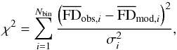${\mathit{\chi }}^{\mathrm{2}}\mathrm{=}\sum _{\mathit{i}\mathrm{=}\mathrm{1}}^{{\mathit{N}}_{\mathrm{bin}}}\frac{{\mathrm{(}{\overline{\mathrm{FD}}}_{\mathrm{obs}\mathit{,i}}\mathrm{-}{\overline{\mathrm{FD}}}_{\mathrm{mod}\mathit{,i}}\mathrm{)}}^{\mathrm{2}}}{{\mathit{\sigma }}_{\mathit{i}}^{\mathrm{2}}}\mathit{,}$(39)where N_bin = 356 is the total number of retained bins, subscript i is the bin identifier, ${\overline{\mathrm{FD}}}_{\mathrm{obs}\mathit{,i}}$ and ${\overline{\mathrm{FD}}}_{\mathrm{mod}\mathit{,i}}$ are the average values of the observational and modeled Galactic FDs, respectively, within bin i, and σ_i is the uncertainty in ${\overline{\mathrm{FD}}}_{\mathrm{obs}\mathit{,i}}$ (estimated in Appendix A). We also define the reduced χ² parameter, 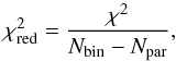${\mathit{\chi }}_{\mathrm{red}}^{\mathrm{2}}\mathrm{=}\frac{{\mathit{\chi }}^{\mathrm{2}}}{{\mathit{N}}_{\mathrm{bin}}\mathrm{-}{\mathit{N}}_{\mathrm{par}}}\mathit{,}$(40)where N_par is the number of free parameters entering the considered magnetic field model. The advantage of using ${\mathit{\chi }}_{\mathrm{red}}^{\mathrm{2}}$ instead of χ² is that ${\mathit{\chi }}_{\mathrm{red}}^{\mathrm{2}}$ gives a more direct idea of how good a fit is. In principle, a fit with ${\mathit{\chi }}_{\mathrm{red}}^{\mathrm{2}}\mathrm{\approx }\mathrm{1}$ [${\mathit{\chi }}_{\mathrm{red}}^{\mathrm{2}}\mathrm{\gg }\mathrm{1}$] is good [bad]. Here, however, because of the large uncertainties in σ_i (see Appendix A), we do not ascribe too much reality to the absolute ${\mathit{\chi }}_{\mathrm{red}}^{\mathrm{2}}$, but we rely on the relative ${\mathit{\chi }}_{\mathrm{red}}^{\mathrm{2}}$ to rank the different fits by relative likelihood. In the following, the minimum values of χ² and ${\mathit{\chi }}_{\mathrm{red}}^{\mathrm{2}}$ are denoted by ${\mathit{\chi }}_{\min }^{\mathrm{2}}$ and ${\mathit{\chi }}_{\mathrm{red}\mathit{,}\min }^{\mathrm{2}}$, respectively.

Because of the relatively large number of free parameters, a systematic grid search over the N_par-dimensional parameter space would be prohibitive in terms of computing time. Therefore, we opt for the much more efficient MCMC sampling method. We employ two different versions of this method, corresponding to two different implementations of the Metropolis-Hastings algorithm (Metropolis et al. 1953; Hastings 1970): in the first version, the proposal distribution is centered on an educated guess for the best-fit solution, whereas in the second version (random walk Metropolis-Hastings algorithm), the proposal distribution is centered on the current point of the Markov chain (see, e.g., Robert 2015, and references therein). After verifying that both versions lead to the same results (within the Monte Carlo uncertainties) and remarking that the second version is systematically faster, we use only the second version in most of our numerous trial runs. However, in our last series of runs (leading to the final results listed in Table 2), we use again both versions as a reliability check.

For every χ² minimization, we run several, gradually more focused simulations, whose sequence is optimized by trial and error to converge as fast as possible to the correct target distribution. The key is to find a good compromise between sufficiently broad coverage of the parameter space (to make sure the absolute χ² minimum is within reach) and sufficiently narrow bracketing of the minimum-χ² solution (to recover the target distribution in a manageable time). We begin with a simulation having broad proposal (q) and target (π) distributions. For the former, we generally adopt a N_par-dimensional Gaussian with adjustable widths, which we take initially large enough to encompass all plausible parameter values. For the latter, we adopt π ∝ exp(−χ²/ 2T), with T tuned in parallel with the Gaussian widths to achieve the optimal acceptance rate for the next proposed point in the Markov chain (see, e.g., Roberts et al. 1997; Jaffe et al. 2010). Once a likelihood peak clearly emerges, we start a new simulation with narrower q (smaller Gaussian widths) and π (smaller T) and with the starting point of the Markov chain close to the emerging peak. We repeat the procedure a few times until T = 1, as ultimately required. Note that we prefer to keep a handle on how the proposal and target distributions are gradually narrowed down, rather than implement one of the existing adaptive algorithms that can be found in the literature.

We monitor convergence to the target distribution by visually inspecting the evolution of the histogram, the running mean, and the minimum-χ² (i.e., best-fit) value of each parameter as well as the histogram of χ² itself. We stop sampling when a stationary state appears to have been reached, and after checking that the best-fit value of each parameter has achieved an accuracy better than 10% of the half-width of its 1σ confidence interval⁷. The latter is taken to be the projection onto the parameter’s axis of the N_par-dimensional region containing the 68% points of the Markov chain (or second half thereof) with the lowest χ². For our final results (listed in Table 2), we simulate multiple Markov chains in parallel, with overdispersed starting points, we discard the first halves of the chains to skip the burn-in phase, and relying on the Gelman-Rubin convergence diagnostic (Gelman & Rubin 1992), we consider that our chains have converged when, for each parameter, the variance of the chain means has dropped below 10% of the mean of the chain variances, or nearly equivalently, when the potential scale reduction factor, $\sqrt{\mathit{R̂}}$, has dropped below 1.05.

As mentioned at the end of Sect. 4.1, we apply our fitting procedure first to the symmetric and antisymmetric components of the Galactic FD separately, then to the total (symmetric + antisymmetric) Galactic FD. The uncertainties in ${\overline{\mathrm{FD}}}_{\mathrm{obs}\mathit{,}\mathrm{S}\mathit{,i}}$ and ${\overline{\mathrm{FD}}}_{\mathrm{obs}\mathit{,}\mathrm{A}\mathit{,i}}$, σ_S,i and σ_A,i, are related to the uncertainties in ${\overline{\mathrm{FD}}}_{\mathrm{obs}\mathit{,i}}$ and ${\overline{\mathrm{FD}}}_{\mathrm{obs}\mathit{,}\mathrm{-}\mathit{i}}$, σ_i and σ_{− i}, through 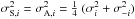${\mathit{\sigma }}_{\mathrm{S}\mathit{,i}}^{\mathrm{2}}\mathrm{=}{\mathit{\sigma }}_{\mathrm{A}\mathit{,i}}^{\mathrm{2}}\mathrm{=}\frac{\mathrm{1}}{\mathrm{4}}\mathrm{(}{\mathit{\sigma }}_{\mathit{i}}^{\mathrm{2}}\mathrm{+}{\mathit{\sigma }}_{\mathrm{-}\mathit{i}}^{\mathrm{2}}\mathrm{)}$, where subscript −i is used to denote the bin that is the symmetric of bin i with respect to the midplane.

5. Results

5.1. Preliminary remarks

Before considering any particular magnetic field model, let us make a few general remarks that will guide us in our exploration of the different parameter spaces and help us optimize the Metropolis-Hastings MCMC algorithm used for our fitting procedure (see Sect. 4.2) – in particular, by making an informed initial choice for the proposal distribution, q. These remarks will also enable us to check a posteriori that the best-fit solutions do indeed conform to our physical expectation.

First, the all-sky maps of the symmetric and antisymmetric components of the bin-averaged observational Galactic Faraday depth, ${\overline{\mathrm{FD}}}_{\mathrm{obs}\mathit{,}\mathrm{S}}$ and ${\overline{\mathrm{FD}}}_{\mathrm{obs}\mathit{,}\mathrm{A}}$, displayed in the middle and bottom panels of Fig. 3, show that ${\overline{\mathrm{FD}}}_{\mathrm{obs}\mathit{,}\mathrm{A}}$ is broadly distributed, both in latitude and in longitude, while the distribution of ${\overline{\mathrm{FD}}}_{\mathrm{obs}\mathit{,}\mathrm{S}}$ is thinner in latitude⁸ and more heavily weighted toward the outer Galaxy. This suggests that the symmetric field, B_S, has a flatter distribution, which extends out to larger radii, while the antisymmetric field, B_A, has a more spherical distribution, which extends up to larger heights. Clearly, these different distributions support our choosing disk-field models (Ad1, Bd, Dd) to describe B_S and halo-field models (A1, B, C, D) to describe B_A. Furthermore, out of our four halo-field models, we may already anticipate that model C, where the field strength has the most spherical distribution (see Fig. 4c), is the best candidate to represent the antisymmetric field. This expectation is in line with the notion that models A, B, and D, where low-| z | field lines are nearly horizontal (see Figs. 4a, b, d), could easily be explained by a disk dynamo (together with a galactic wind advecting the disk-dynamo field into the halo), which is known to favor symmetric fields (see Paper I)⁹.

Second, the multiple sign reversals with longitude observed in the map of ${\overline{\mathrm{FD}}}_{\mathrm{obs}\mathit{,}\mathrm{S}}$ (middle panel of Fig. 3) suggest that B_S is non-axisymmetric. In reality, an axisymmetric magnetic field could very well lead to longitudinal FD reversals (in addition to the two reversals, toward ℓ ≈ 0° and ℓ ≈ 180°, naturally associated with an axisymmetric, nearly azimuthal field) if it reverses direction with radius. As a general rule, if the axisymmetric field reverses n times with radius, FD can reverse up to 2 (n + 1) times with longitude. A case in point is provided by the concentric-ring model of Rand & Kulkarni (1989), where the field is purely azimuthal and reverses direction from one ring to the next. What about our three disk-field models? As explained in Sect. 3.2, model Ad1 is inherently bisymmetric. Model Dd has no radial field reversals (see Eqs (18)–(19) for the poloidal field and Eq. (28) for the azimuthal field), so it cannot lead to more than two longitudinal FD reversals. Model Bd has one reversal of B_z at radius r₁ (see Eq. (35)), which must be accompanied by one reversal of B_ϕ at a slightly smaller radius (see Eq. (28)); the resulting radial reversal of the total field could account for a maximum of four longitudinal FD reversals, which is still short of the observed number of reversals. Ultimately, it appears that none of our axisymmetric disk-field models is likely to reproduce the general sign pattern of the ${\overline{\mathrm{FD}}}_{\mathrm{obs}\mathit{,}\mathrm{S}}$ map. To strengthen this conclusion, we note that our axisymmetric disk-field models would also be hard-pressed to reproduce the preponderance of the outer Galaxy in the ${\overline{\mathrm{FD}}}_{\mathrm{obs}\mathit{,}\mathrm{S}}$ map.

Altogether, the remaining good candidates are model C for the antisymmetric field, B_A, and model Ad1 plus the non-axisymmetric versions of models Bd and Dd for the symmetric field, B_S. If we retain only axisymmetric (m = 0) and bisymmetric (m = 1) models, and label them with the value of the azimuthal wavenumber, m, appended to the letters of the models, our full list reduces to models A1, B0, B1, C0, C1, D0, and D1 for B_A and models Ad1, Bd0, Bd1, Dd0, and Dd1 for B_S, amongst which the good candidates are models C0 and C1 for B_A and models Ad1, Bd1, and Dd1 for B_S.

The impact of the model parameters on the ${\overline{\mathrm{FD}}}_{\mathrm{mod}}$ map is discussed in detail in Appendix B, and a summary of the discussion of the axisymmetric (m = 0) case is provided in Table 1.

5.2. Best fits

We consider 35 models of the total magnetic field, corresponding to all the possible combinations of one of the 7 antisymmetric halo-field models, A1, B0, B1, C0, C1, D0, and D1, with one of the 5 symmetric disk-field models, Ad1, Bd0, Bd1, Dd0, and Dd1. We apply the fitting procedure described in Sect. 4.2 to each of our 35 total-field models. As expected, we find that 6 total-field models have significantly lower ${\mathit{\chi }}_{\mathrm{red}\mathit{,}\min }^{\mathrm{2}}$ than the other models, and that they correspond exactly to the 6 combinations of good candidates identified in Sect. 5.1, namely, the combinations of C0 or C1 with Ad1, Bd1, or Dd1. The ${\mathit{\chi }}_{\mathrm{red}\mathit{,}\min }^{\mathrm{2}}$ values, the best-fit parameter values, and the 1σ confidence intervals (in the sense defined in Sect. 4.2) of these 6 total-field models are listed in Table 2.

A first glance at the last column of Table 2 suggests that our ${\mathit{\chi }}_{\mathrm{red}\mathit{,}\min }^{\mathrm{2}}$ values might be too large to qualify for good fits. However, one has to remember that the exact values of ${\mathit{\chi }}_{\mathrm{red}}^{\mathrm{2}}$ should not be taken too seriously; most importantly, they should not be considered individually, but only relative to each other as a means of ranking the different models.

On the basis of this ranking, it emerges that (1) the three total-field models with a bisymmetric halo field (described by model C1; last three combinations in Table 2) perform systematically better than the three total-field models with an axisymmetric halo field (described by model C0; first three combinations in Table 2); and (2) for each halo-field model, the three disk-field models (Ad1, Bd1, Dd1) are nearly equally good. The closeness of the three best fits for each halo-field model lends credence to their being the true absolute best fits, corresponding to the true absolute χ² minima. The differences between the three best fits are smaller when the halo field is bisymmetric than when it is axisymmetric, and in either case, models Ad1 and Bd1 tend to lead to the closer best fits. This follows from the similarity in the shape of their field lines outside the centered vertical cylinder of radius r₁ = 3 kpc (see Figs. 4a and b), it being clear that the interior of the cylinder gives but a small overall contribution to the ${\overline{\mathrm{FD}}}_{\mathrm{mod}}$ maps.

The preference for a bisymmetric halo field can be understood as follows¹⁰: a bisymmetric field leads to field reversals along most lines of sight. The exact locations of the field reversals, and hence the net result of integrating B_∥ along the different lines of sight (see Eq. (2)), and ultimately the appearance of the ${\overline{\mathrm{FD}}}_{\mathrm{mod}}$ maps, depend sensitively on the precise orientation angle of the bisymmetric pattern, ϕ_⋆. In other words, ϕ_⋆ offers a very special degree of freedom, which makes it possible to produce a great variety of ${\overline{\mathrm{FD}}}_{\mathrm{mod}}$ maps. By fine-tuning the value of ϕ_⋆, it is generally possible to bring the ${\overline{\mathrm{FD}}}_{\mathrm{mod}}$ maps into (relative) good agreement with the observational ${\overline{\mathrm{FD}}}_{\mathrm{obs}}$ map.

Let us now discuss the best-fit values of the free parameters, starting with the parameters governing the field strength distribution (B₁, H, L, ϕ_⋆) and the curvature of parabolic field lines in models Ad1, C0, and C1 ($\sqrt{\mathit{a}}$), and continuing with the parameters governing the spiral shape of field lines (p₀, H_p, L_p). The 1σ confidence intervals and the correlations between parameters are discussed in Appendix C.

When the halo field is bisymmetric, it has a much larger normalization field strength, B₁ (by a factor ≈ 25−50) than when it is axisymmetric, and the associated disk field also has a larger B₁ (by a factor ≈ 2−15). The larger (B₁)_halo and (B₁)_disk obtained with a bisymmetric halo field are needed to make up for the azimuthal modulation of the halo field and for the associated field reversals, which lead to cancelation in the line-of-sight integration of B_∥. The strong increase in B₁ is accompanied by a weaker decrease (by a factor ≈ 1−4) in the scale height at r₁, H, and in the scale length at z₁, L. At the same time, the curvature parameter of parabolic field lines, $\sqrt{\mathit{a}}$, decreases slightly (by a factor ≈ 1.2−2) for the halo field and more significantly (by a factor ≈ 5) for the disk field in model Ad1. The origin of these trends will become clearer in Sect. 5.3.

More quantitatively, the halo field always has a short scale length at z₁ (L ≈ (2−5) kpc). The disk field has a longer scale length at z₁ (L ≈ (3−10) kpc in model Dd1), or a short scale height at r₁ (H ≈ 50 pc in model Ad1 and H ≈ (100−300) pc in model Bd1) combined with an outward flaring of field lines ($\sqrt{\mathit{a}}\mathrm{\approx }\mathrm{1}\mathit{/}\mathrm{(}\mathrm{1}\mathrm{-}\mathrm{5}\mathrm{)}\mathrm{kpc}$ in model Ad1 and n = 2 in model Bd1). The scale lengths in models C0, C1, and Dd1 are realistic, whereas the scale heights in models Ad1 and Bd1 are probably too short, even when their outward increase due to the flaring of field lines is taken into account – for instance, the scale height at the Sun is only ≈ (140−360) pc in model Ad1 and ≈ (120−440) pc in model Bd1.

With the above values of L, H, $\sqrt{\mathit{a}}$, and n, the ratio (B₁)_halo/ (B₁)_disk can be adjusted in such a way that the halo [disk] field imposes its vertical antisymmetry [symmetry] to the Galactic FD toward the inner [outer] halo, as required by the north-south symmetry properties of the ${\overline{\mathrm{FD}}}_{\mathrm{obs}}$ sky (see Sect. 2.2). The resulting B₁ are generally realistic, although when the halo field is bisymmetric, the total field outside r = 3 kpc can become quite strong at the crests of the azimuthal modulation (up to ≈ 200 μG and ≈ 150 μG at (r = 3 kpc,z = 0) in the combinations C1-Ad1 and C1-Bd1, respectively)¹¹. On the other hand, the large (B₁)_disk (≈ 30 μG) in C1-Ad1 and C1-Bd1 are not inconsistent with our imposed range of [1,2] μG for the local field strength, B_⊙ (see Sect. 4.1): indeed, it suffices for the Sun to fall close to a node of the sinusoidal variation of the disk field. Neither is the very small (B₁)_disk (≈ 0.06 μG) in C0-Dd1 problematic, as (B₁)_disk is only the peak vertical component of the disk field at (r₁ ≤ L,z₁ = ± 1.5 kpc) (see Eq. (36)), which is much weaker than the total field near the Galactic plane.

In each total-field model, the parameters governing the spiral shape of field lines have common values for the disk and halo fields. The pitch angle at the origin, p₀, is always negative and small (≈ (− 9°)−(−7°)), corresponding to a trailing magnetic spiral with nearly azimuthal field at the origin (see Eq. (28)). | p₀ | is slightly smaller when the halo field is axisymmetric, and accordingly the field is slightly more azimuthal. The scale length of the winding function, L_p, is always very large (best-fit value ≳ 40 kpc), implying that the field remains nearly azimuthal out to large radii. In contrast, the scale height of the winding function, H_p, is very sensitive to the azimuthal structure of the halo field: when the halo field is axisymmetric, H_p is greater than the free-electron scale height, H_e ≃ 1.3 kpc (see Sect. 4.1), so that the field remains nearly azimuthal across the free-electron layer (where the Galactic FD arises; see Eq. (2)), while in the case of a bisymmetric halo field, H_p is comparable to H_e, so that the field acquires a significant poloidal component within the free-electron layer. The reason for this dichotomy as well as for the slight difference in p₀ is easily understood: in the axisymmetric case, the field must remain nearly azimuthal in order to reproduce the rough east-west antisymmetry in the ${\overline{\mathrm{FD}}}_{\mathrm{obs}}$ sky, whereas in the bisymmetric case, the field can a priori remain nearly azimuthal or become more poloidal (see last paragraph of Sect. 2.2).

5.3. Faraday-depth maps

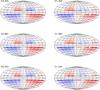Fig. 5 All-sky maps of the bin-averaged modeled Galactic Faraday depth, ${\overline{\mathrm{FD}}}_{\mathrm{mod}}$, for the six best-fit magnetic field models listed in Table 2. The left and right columns are for a halo field described by model C0 (axisymmetric) and C1 (bisymmetric), respectively, while the top, middle, and bottom rows are for a disk field described by models Ad1, Bd1, and Dd1, respectively. The coordinate system and the color code of each map are the same as in Fig. 3.

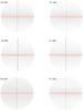Fig. 6 Synthetic maps of the magnetic orientation bars, inferred from the synchrotron polarized emission, of our Galaxy seen edge-on from the position (r → ∞,ϕ = 90°,z = 0), for the six best-fit magnetic field models listed in Table 2. The left and right columns are for a halo field described by model C0 (axisymmetric) and C1 (bisymmetric), respectively, while the top, middle, and bottom rows are for a disk field described by models Ad1, Bd1, and Dd1, respectively. Each map covers a circular area of radius 15 kpc, the trace of the Galactic plane is indicated by the horizontal, red, solid line, and the rotation axis by the vertical, black, dot-dashed line. All magnetic orientation bars have the same length, and their shade of grey scales logarithmically with the polarized intensity.

Figure 5 presents the all-sky ${\overline{\mathrm{FD}}}_{\mathrm{mod}}$ maps obtained with the best-fit parameter values of the six magnetic field models listed in Table 2. These modeled maps are to be compared with the observational map of ${\overline{\mathrm{FD}}}_{\mathrm{obs}}$ in the top panel of Fig. 3.

As expected, the ${\overline{\mathrm{FD}}}_{\mathrm{mod}}$ maps obtained with the axisymmetric halo-field model C0 (left column in Fig. 5) are simpler and show less spatial structure than those obtained with the bisymmetric halo-field model C1 (right column), and for each halo-field model, the three disk-field models, Ad1 (top row), Bd1 (middle row), and Dd1 (bottom row), make very little difference, with variations noticeable only at low latitudes. Otherwise, all ${\overline{\mathrm{FD}}}_{\mathrm{mod}}$ maps reproduce the rough east-west antisymmetry as well as the rough north-south antisymmetry [symmetry] toward the inner [outer] Galaxy. The east-west pattern is actually slightly shifted westward (by ≲ 10°), with the longitudes of sign reversals occurring not exactly at ℓ = 0°,180°, but at slightly smaller longitudes. This westward shift, which is also apparent in the observational ${\overline{\mathrm{FD}}}_{\mathrm{obs}}$ map, is due to the slightly negative pitch angle. Furthermore, when the halo field is bisymmetric, the westward shift is compounded by an east-west asymmetry arising from the azimuthal modulation of the halo field; this asymmetry is most striking between the (very dim) north-east and (less dim) north-west outer quadrants.

The ${\overline{\mathrm{FD}}}_{\mathrm{mod}}$ values in the north outer quadrants are systematically too small, particularly when the halo field is axisymmetric (left column in Fig. 5) and in the north-east outer quadrant when the halo field is bisymmetric (right column). The problem arises because the contributions from the symmetric disk field and from the antisymmetric halo field partly cancel out in the north outer quadrants, while they add up constructively in the south outer quadrants. Since the disk-field contribution must be dominant toward the outer Galaxy (see Sect. 2.2), the problem can be alleviated either by enhancing the disk-field contribution or by reducing the halo-field contribution toward the outer Galaxy, while maintaining the dominance of the halo field toward the inner Galaxy. Such tuning is more easily achieved with bisymmetric fields, which possess the degree of freedom to orient their azimuthal pattern in favor of either the outer Galaxy (for the disk field) or the inner Galaxy (for the halo field). This is the main reason why bisymmetric field models lead to lower ${\mathit{\chi }}_{\mathrm{red}\mathit{,}\min }^{\mathrm{2}}$ than their axisymmetric counterparts (most strikingly for disk-field models, whose axisymmetric versions were dropped from the discussion earlier on) and why the ${\overline{\mathrm{FD}}}_{\mathrm{mod}}$ maps obtained with model C1 are in slightly better visual agreement with the observational ${\overline{\mathrm{FD}}}_{\mathrm{obs}}$ map than the ${\overline{\mathrm{FD}}}_{\mathrm{mod}}$ maps obtained with model C0.

We are now in a position to better understand two of the more subtle results presented in Sect. 5.2. First, the possibility to orient the azimuthal pattern of the halo field in model C1 in favor of the inner Galaxy explains why, when going from model C0 to model C1, (B₁)_halo can increase more than (B₁)_disk without the halo field imposing its north-south antisymmetry to the outer Galaxy. Second, the lack of orientability for the halo field in model C0 implies that combinations with C0 (first three in Table 2) must rely more heavily on the disk field to favor the outer Galaxy; this is why they are found to have larger best-fit values for the parameters H_disk (in model Bd1), L_disk (in model Dd1), and a_disk (in model Ad1) than combinations with C1 (last three in Table 2).

5.4. Synchrotron polarisation maps

Having shown that the six best-fit magnetic field models listed in Table 2 reproduce the observational ${\overline{\mathrm{FD}}}_{\mathrm{obs}}$ map reasonably well, we now use them to generate synthetic synchrotron polarization maps of our Galaxy as would be seen by an external edge-on observer. The procedure is similar to that described in Paper I: for each of our six best-fit magnetic field models, we compute the synchrotron emissivity, $\mathrm{ℰ}\mathrm{\propto }{\mathit{n}}_{\mathrm{rel}}{\mathit{B}}_{\mathrm{\perp }}^{\mathrm{(}\mathit{\gamma }\mathrm{+}\mathrm{1}\mathrm{)}\mathit{/}\mathrm{2}}$, throughout the Galaxy, where B_⊥ is the magnetic field component perpendicular to the line of sight, n_rel is the density of relativistic electrons (assumed to be ∝ B²), γ is the power-law index of the relativistic-electron energy spectrum (set to γ = 3), and the value of the proportionality factor is irrelevant. We also compute the associated Stokes parameters U and Q, knowing that synchrotron emission is (partially) linearly polarized perpendicular to B_⊥ and assuming that the intrinsic degree of linear polarization is uniform throughout the Galaxy. We then integrate U and Q along a large number of sightlines covering the Galaxy to produce grids of polarized intensity and polarization direction. Finally, we rotate every polarization direction by 90° to obtain the so-called magnetic orientation bar, i.e., the headless vector giving the line-of-sight–average orientation of B_⊥, and we plot it in a greyscale that varies logarithmically with the polarized intensity. The resulting synchrotron polarization maps, which do not include any Faraday rotation, Faraday depolarization or beam depolarization effects, are displayed in Fig. 6 for an external observer located at (r_obs → ∞,ϕ_obs = 90°,z_obs = 0). Their variation with ϕ_obs is briefly discussed at the end of the section.

We first note that the polarization maps obtained with the bisymmetric halo-field model C1 (right column in Fig. 6) are perfectly symmetric with respect to the rotation axis, while those obtained with the axisymmetric halo-field model C0 (left column) are only approximately symmetric. Indeed, in the former case, the total field is the superposition of a bisymmetric halo field + a bisymmetric disk field, so the total field vector is antisymmetric with respect to the rotation axis and the magnetic orientation bars form a symmetric pattern. In the latter case, the total field is the superposition of an axisymmetric halo field + a bisymmetric disk field, so the total field vector is neither perfectly symmetric nor perfectly antisymmetric with respect to the axis and the magnetic orientation bars do not form a perfectly symmetric pattern; the reason why the polarization maps look approximately symmetric is because (1) most regions in space are dominated by either the axisymmetric halo field or the bisymmetric disk field; and (2) asymmetries in the polarized intensity are toned down by the logarithmic greyscale.

When the halo field is axisymmetric (left column in Fig. 6), the magnetic orientation bars remain nearly horizontal almost everywhere (or at least up to | z | ≈ 8 kpc in model C0-Dd1; bottom-left panel) and no X shape emerges. In contrast, when the halo field is bisymmetric (right column), the magnetic orientation bars are nearly horizontal only in a thick layer along the Galactic plane (| z | ≲ (4−5) kpc) and they turn into a V shape (i.e., the upper or lower part of an X) on either side of this layer. This split result is an immediate consequence of the dichotomy in the values of the scale height of the winding function, H_p, noted and explained in Sect. 5.2: with an axisymmetric halo field, H_p is large (≳ 4 kpc) and the field remains nearly azimuthal up to high | z |, leading to nearly horizontal magnetic bars; with a bisymmetric halo field, H_p is much smaller (≃ 1.2 kpc) and the field turns poloidal at much lower | z |, leading to an X-shape pattern.

Here, too, the impact of the disk-field model is much weaker than that of the halo-field model. The most obvious, yet rather minor, difference between the three disk-field models is that the region of nearly horizontal magnetic bars is somewhat broader with models Ad1 (top row in Fig. 6) and Bd1 (middle row) than with model Dd1 (bottom row). Another difference arises in model Bd1: the magnetic bars along the rotation axis are vertical, and fine-resolution maps show that they remain nearly vertical out to projected distances of a few 100 pc from the axis. This is because model Bd1 has a strong concentration of nearly vertical field lines around the axis (see Fig. 4b), which dominates the line-of-sight integration of the synchrotron emissivity.

The above conclusions are quite general, but the details of the polarization maps depend on the viewing angle, ϕ_obs, especially when the halo field is bisymmetric. First, while the layer of nearly horizontal magnetic bars maintains a roughly constant thickness (≃ (4−5) kpc), its grey-shade distribution, which reflects the polarized-intensity distribution, varies with ϕ_obs. This is easily understood if one remembers that the polarized intensity depends sensitively on B_⊥ near the crests of the azimuthal modulation. Second, in the X-shape region, the opening angle of the upper and lower V that compose the X changes with ϕ_obs, as expected for a projected bisymmetric structure; in addition, there may be a range of ϕ_obs for which magnetic bars near the axis slope down toward the midplane instead of pointing outwards, such that the upper and lower V actually turn into W. The latter arises when the dominant portions of the crest regions occur in the near-east and far-west parts of the Galaxy, where the Galactic differential rotation tilts the projected orientation of an initially X-shape poloidal field toward, and even past, the vertical.

In summary, amongst our six best-fit magnetic field models, the three models with a bisymmetric halo field (model C1; right column in Fig. 6) produce an X-shape pattern in synchrotron polarisation maps, while those with an axisymmetric halo field (model C0; left column) do not.

5.5. Comparison with previous work

Other authors have recently set out to determine, or at least constrain, the magnetic field structure in the Galactic halo. We now briefly discuss their models, in comparison to ours.

Sun et al. (2008) modeled the large-scale magnetic field of our Galaxy as the superposition of a disk field and a halo field, which they constrained with an all-sky map of extragalactic RMs. Their disk field was assumed to be purely horizontal, following a logarithmic spiral (constant pitch angle), symmetric in z, and either axisymmetric with radial reversals or bisymmetric, while their halo field was assumed to be purely azimuthal, in the form of a torus on either side of the Galactic plane, antisymmetric in z, and axisymmetric. Clearly, the purely azimuthal, axisymmetric halo field is automatically divergence-free, but the purely horizontal disk field is not – for instance, in the axisymmetric case, the divergence-free condition implies B_r ∝ 1 /r, which rules out radial reversals. Sun et al. (2008) found reasonably good fits to the RM data with axisymmetric disk fields having a pitch angle of −12° (somewhat larger in absolute value than in our best-fit models), whereas they found no good fits with bisymmetric disk fields. This result is at odds with our conclusion that bisymmetric disk fields provide better fits. The discrepancy can be mostly traced back to Sun et al.’s neglect of the divergence-free condition, which allows their axisymmetric disk field to undergo radial reversals and, therefore, makes it easier to reproduce the RM data (see our discussion in the third paragraph of Sect. 5.1).

Another problem with Sun et al.’s (2008) study is its reliance on the NE2001 model for the free-electron density, which underestimates the free-electron scale height, H_e (see Sect. 4.1). An unrealistically strong halo field (≈ 10 μG) is then necessary to account for the high-latitude extragalactic RMs, which, in turn, requires truncating the relativistic-electron distribution at | z | ≈ 1 kpc to avoid excessive synchrotron emission from the halo. The problem was fixed by Sun & Reich (2010), with the adoption of Gaensler et al.’s (2008) upward revision of H_e; this led to a more realistic halo field (≈ 2 μG) and obviated the need to artificially truncate the relativistic-electron distribution. The revised model of Sun & Reich (2010) was then used by Sun & Reich (2012) to simulate the synchrotron emission of spiral galaxies similar to our Galaxy and study their polarization properties for various observing angles.

Later, Sun et al. (2015) noted that Sun & Reich’s (2010) model underpredicted the Galactic FD at latitude b ≳ 50°. They argued that the halo field needed to have a vertical component, and they showed that the inclusion of a dipole field with B_z = −0.2 μG at the Sun was enough to bring the predicted Galactic FD at b ≳ 50° up to the observed level. However, they did not discuss how the Galactic FD at lower latitudes was affected, nor did they specify whether the global fit to the RM data (measured through ${\mathit{\chi }}_{\mathrm{red}}^{\mathrm{2}}\mathrm{)}$ was actually improved.

The vertical component of the halo field in the solar neighborhood has been the subject of a few other studies. Based on the structure of their NVSS RM map at high | b |, Taylor et al. (2009) estimated B_z ≃ −0.14 μG above the midplane and B_z ≃ 0.30 μG below the midplane. Mao et al. (2010), for their part, relied on a set of more than 1000 WRST/ATCA extragalactic RMs at | b | ≥ 77°; after discarding outliers and anomalous RM regions, they derived B_z ≃ 0.00 μG toward the north Galactic pole (with a 3σ upper limit on | B_z | of 0.07 μG) and B_z ≃ + 0.31 μG toward the south Galactic pole. The south value is very close to that of Taylor et al. (2009), but the north value is incompatible with those of Taylor et al. (2009) and Sun et al. (2015). Nevertheless, the results of both Taylor et al. (2009) and Mao et al. (2010) are consistent with the notion that the large-scale Galactic magnetic field is the superposition of a symmetric disk field and an antisymmetric halo field, whose contributions to high-| b | RMs cancel out above the midplane and add up below it. In Taylor et al. (2009) the symmetric contribution would dominate (see footnote 4), while in Mao et al. (2010) both contibutions would be comparable.

For comparison, in each of our six best-fit models, the average B_z toward either Galactic pole, as inferred from the ratio of Galactic FD to free-electron column density, is positive. The contribution from the halo field is always positive and dominant. The weaker contribution from the disk field is negative [positive] above [below] the midplane in models Ad1 and Bd1, and vice-versa in model Dd1. This is a direct consequence of imposing (B_r)_⊙ < 0 (see Sect. 4.1), which, in view of the shape of poloidal field lines, implies (B_r)_disk < 0 and (B_z)_disk < 0 [(B_z)_disk > 0] in the northern [southern] halo in models Ad1 and Bd1, and the opposite in model Dd1, where poloidal field lines reverse direction at z = z₁ (see Eq. (18)). As a result, the average B_z is stronger toward the south Galactic pole with models Ad1 and Bd1 (as found by both Taylor et al. 2009 and Mao et al. 2010) and stronger toward the north Galactic pole with model Dd1 (in conflict with the measured high-|b| RMs). Hence, high-| b | RMs give more credence to models Ad1 and Bd1 than model Dd1.

Additional constraints on the halo field were obtained by Mao et al. (2012), based on 641 extragalactic RMs at longitude 100° < ℓ < 117° and latitude |b| < 30°. The vast majority of the RMs are negative, as expected for a predominantly azimuthal, clockwise magnetic field. The RM latitudinal distribution is approximately symmetric up to | b | ≃ 15°, and it becomes increasingly asymmetric at higher | b |, with significantly larger | RM | in the southern hemisphere. Mao et al. (2012) noted that the RM distribution at | b | ≲ 15° is consistent with a symmetric disk field in the Perseus arm. They also showed that the RM distribution at | b | ≳ 15° could be reproduced with a purely azimuthal halo field confined to the radial range [8.8,10.3] kpc (assuming r_⊙ = 8.4 kpc), i.e., between the local and Perseus arms, and to the vertical ranges ± [0.8,2.0] kpc, with B_ϕ = 2 μG [7 μG] above [below] the midplane. Here, we see that the RM latitudinal distribution can also be explained by the superposition of a symmetric disk field and an antisymmetric halo field, such that the disk field contribution largely dominates at | b | ≲ 15° and the halo field contribution becomes increasingly important at higher | b |, opposing the disk field contribution in the northern hemisphere and reinforcing it in the southern hemisphere. In our study, the six best-fit models yield negative Galactic FD throughout the 17°×60° area surveyed by Mao et al. (2012), except for slightly positive values at b ≳ 15° with model C1, and they reproduce the observed trends of RM versus b quite well.

The first, and to our knowledge only, authors to include an X-shape component in their model of the large-scale Galactic magnetic field are Jansson & Farrar (2012a,b). The disk field in their model is symmetric in z, purely horizontal, and composed of a ring between radii 3 kpc and 5 kpc plus 8 logarithmic spirals between 5 kpc and 20 kpc, with a common pitch angle of −11.5° and separate field strengths constrained by global magnetic flux conservation. The halo field has two axisymmetric components: a purely azimuthal field with opposite signs and different strengths on both sides of the midplane (similar to the halo field of Sun et al. 2008; Sun & Reich 2010, but more general because not perfectly antisymmetric in z), and a purely poloidal field with an X shape (similar to the poloidal field in our model C, but with straight field lines and a cusp at z = 0). These two components are unrelated, in contradiction with dynamo theory which predicts that azimuthal field is generated from poloidal field and vice-versa. Jansson & Farrar (2012a,b) found that the inclusion of an X-shape component improved the global fit to their data set, which contained the WMAP7 Galactic synchrotron emission map together with a collection of more than 40 000 extragalactic RMs. The improvement brought about by an X-shape poloidal field is also obvious in our study, where the pitch angle is found to have non-zero values to a high confidence level.

6. Discussion

In this paper, we took a first important step in our efforts to understand the structure of the large-scale magnetic field in the Galactic halo, with special attention to the possibility of uncovering an X-shape magnetic configuration, as observed in external edge-on spiral galaxies. We applied the analytical magnetic field models developed in Paper I to the disk and halo of our Galaxy, on the basis that these models can describe a broad range of spiraling, possibly X-shape magnetic fields, including purely horizontal and purely vertical fields as limiting cases. We considered 35 models of the total (halo + disk) magnetic field, each composed of one of our 7 antisymmetric halo-field models, A1, B0, B1, C0, C1, D0, and D1, plus one of our 5 symmetric disk-field models, Ad1, Bd0, Bd1, Dd0, and Dd1 (where 0 and 1 denote axisymmetric and bisymmetric fields, respectively). For each total-field model, we computed the average Galactic Faraday depth in the 356 bins covering the sky area at | b | ≥ 10°, and we confronted the resulting modeled map of ${\overline{\mathrm{FD}}}_{\mathrm{mod}}$ to the observational map of ${\overline{\mathrm{FD}}}_{\mathrm{obs}}$ displayed in the top panel of Fig. 3 (based on the reconstructed Galactic FD map of Oppermann et al. 2015, from which the contribution from Wolleben et al.’s 2010 magnetized bubble was advantageously removed). The adjustment of ${\overline{\mathrm{FD}}}_{\mathrm{mod}}$ to ${\overline{\mathrm{FD}}}_{\mathrm{obs}}$ was carried out through standard χ² minimization, with the help of MCMC simulations.

We found that the 6 total-field models composed of C0 or C1 (for the halo field) plus Ad1, Bd1, or Dd1 (for the disk field) (listed in Table 2) had significantly lower ${\mathit{\chi }}_{\mathrm{red}\mathit{,}\min }^{\mathrm{2}}$ than any of the other total-field models. Amongst them, models with C1 have slightly lower ${\mathit{\chi }}_{\mathrm{red}\mathit{,}\min }^{\mathrm{2}}$ (2.02−2.08) than models with C0 (2.26−2.42), and they provide a slightly better visual match to the observational ${\overline{\mathrm{FD}}}_{\mathrm{obs}}$ map (see Fig. 5). Neither the value of ${\mathit{\chi }}_{\mathrm{red}\mathit{,}\min }^{\mathrm{2}}$ nor the appearance of the ${\overline{\mathrm{FD}}}_{\mathrm{mod}}$ map is significantly affected by the disk-field model. The only discriminating factor comes from high-| b | RMs, which tend to favor models Ad1 and Bd1 over model Dd1.

Thus, regardless of the bisymmetric disk field, the three models with a bisymmetric halo field perform slightly (but systematically) better with regard to the Galactic FD than the three models with an axisymmetric halo field. As it turns out, the former also produce an X-shape pattern in synchrotron polarisation maps, while the latter lead to nearly horizontal magnetic orientation bars throughout most of the maps (see Fig. 6). As explained in Sects. 5.2 and 5.4, this difference in the polarisation maps stems from the rough east-west antisymmetry in the ${\overline{\mathrm{FD}}}_{\mathrm{obs}}$ sky, which has strong implications for the azimuthal-to-poloidal field ratio: in the axisymmetric case, the field must necessarily be nearly azimuthal up to high | z | – hence the nearly horizontal magnetic orientation bars, whereas in the bisymmetric case, the field can turn poloidal at relatively low | z | – hence the X-shape pattern.

In conclusion, the existing RM data, interpreted with the help of our (hopefully sufficiently general) magnetic field models, suggest that the Galactic halo is slightly more likely to have a bisymmetric field than an axisymmetric field. If the halo field is indeed bisymmetric, it would probably be seen as X-shaped by an external edge-on observer, while it would probably be seen as nearly horizontal if it is instead axisymmetric. We emphasize that the preference found here for a bisymmetric, X-shape halo field cannot be regarded as definite, first because it is based solely on RM data and second because the bisymmetric halo field performs only slightly better than its axisymmetric counterpart.

The results obtained for the disk field – in particular, the finding that the disk field is more likely to be bisymmetric – are even more subject to caution. Indeed, since our original interest was in the halo field, we excluded all sightlines toward the disk (| b | < 10°), and the main reason why we needed to model the disk field was because even sightlines toward the halo must first pass through the disk. By essence, these sightlines miss a sizeable fraction of the disk field, so our analysis can only give partial information on the global properties of the disk field, such as its axisymmetric versus bisymmetric status.

A severe limitation of the RM data arises from the relatively rapid fall-off of the free-electron density with height, which makes it hard to sample the Galactic magnetic field at large distances from the Galactic plane. Therefore, any method relying exclusively on RM data is not particularly well suited to look into the structure of the magnetic field in the Galactic halo. On the other hand, RM data have the unique advantage of containing a sign information, which is required to distinguish between symmetric and antisymmetric models or between axisymmetric and bisymmetric models. Ultimately, RM data provide a unique, albeit limited, set of constraints on the properties of the large-scale magnetic field in the Galactic halo. Obtaining a more complete set of constraints will require fitting our magnetic field models to other types of observations, such as synchrotron total and polarized emission.

Despite the inherent limitation of the RM data to explore the magnetic field structure in the Galactic halo, our investigation offers a first important glimpse. In addition, our search for a good fit to the observational ${\overline{\mathrm{FD}}}_{\mathrm{obs}}$ map led us to improve and refine the analytical magnetic field models of Paper I. Most notably, we derived a more realistic winding function (Eq. (23)), applicable to all our field models, and we regularized the bisymmetric version of model A by assuming a straight, horizontal magnetic field inside a vertical cylinder of radius r₁ centered on the rotation axis (see Eq. (29) for halo fields and Eq. (31) for disk fields). Finally, the method proposed in this paper is interesting in its own right: it contains a number of original features, including a detailed error estimation (see Appendix A), which can be retained for similar investigations. As a possible application, we suggest using our method to study the magnetic field structure in targeted regions of the sky. We also suggest repeating the present analysis when new RM data in the southern hemisphere become available to fill in the gap at δ< −40° in Taylor et al.’s (2009) NVSS catalog¹², and when the nearby objects that significantly perturb the FD sky have been identified, and their FD quantified, through RM synthesis (see Wolleben et al. 2010), such that a more complete and cleaner all-sky ${\overline{\mathrm{FD}}}_{\mathrm{obs}}$ map can be produced.

Acknowledgments

We express our deep gratitude to our colleagues, Tess Jaffe and Pierre Jean, who provided valuable help with the MCMC simulations, and to Maik Wolleben, who kindly sent us the FD data for the Wolleben et al. (2010) bubble.

References

Appendix A: Uncertainty estimation

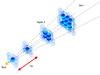Fig. A.1 Schematic drawing illustrating the concept of turbulent cells and layers used in our estimation of σturb,i, the uncertainty in ${\overline{\mathrm{FD}}}_{\mathrm{obs}\mathit{,i}}$ arising from turbulence in the magneto-ionic ISM, for a particular bin i (see Eq. (A.5) and attendant discussion). The Galactic volume subtended by bin i (delimited by the four black dotted lines originating from the Sun) is divided into transverse layers of thickness l (delimited by black solid lines). These layers contain an increasing number of turbulent cells of size l (represented by opaque blue spheres, while transparent blue spheres represent cells falling outside the bin). The distance Ltr from the Sun marks the transition between the so-called nearby layers, which can be completely filled with a single cell, and the distant layers, which enclose several cells.

Fig. A.2 Total uncertainty in ${\overline{\mathrm{FD}}}_{\mathrm{obs}\mathit{,i}}$, σi, as a function of bin identifier, i (thick magenta line), for the 356 bins with latitude | b | ≥ 10°. Also plotted are the two contributions to σi (see Eq. (A.1)), which arise from the reconstruction of Oppermann et al. (2015) (σrec,i; red line) and from turbulence in the magneto-ionic ISM (σturb,i; brown line), respectively. The latter, in turn, is accompanied by its two contributions (see Eq. (A.6)), which arise from the N′ear nearest layers (thin green line) and from the Nlayer,i−N′ear more distant layers (thin blue line), respectively. Bins are ordered by bands of increasing latitude, from b = −90° to 90°, and in each latitude band, by increasing longitude, from ℓ = −180° to 180°. The vertical grey band in the middle corresponds to bins with latitude | b | < 10°, which are excluded from our study.

When using the ${\overline{\mathrm{FD}}}_{\mathrm{obs}}$ map in the top panel of Fig. 3 as our observational reference to model the large-scale magnetic field in the Galactic halo, we have to take two main sources of uncertainty into account: (1) the uncertainty in the reconstructed Galactic FD map of Oppermann et al. (2015), which includes both the measurement errors in the RM data and an extragalactic RM contribution; and (2) the uncertainty due to turbulent fluctuations in the magneto-ionic ISM. If, for each bin i, we denote the corresponding uncertainties in ${\overline{\mathrm{FD}}}_{\mathrm{obs}\mathit{,i}}$ by σ_rec,i and σ_turb,i, respectively, and if we note that the two uncertainties add up quadratically, we can write for the total uncertainty in 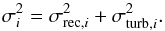${\overline{\mathrm{FD}}}_{\mathrm{obs}\mathit{,i}}$, σ_i: ${\mathit{\sigma }}_{\mathit{i}}^{\mathrm{2}}\mathrm{=}{\mathit{\sigma }}_{\mathrm{rec}\mathit{,i}}^{\mathrm{2}}\mathrm{+}{\mathit{\sigma }}_{\mathrm{turb}\mathit{,i}}^{\mathrm{2}}\mathit{.}$(A.1)We now successively derive the appropriate expressions of ${\mathit{\sigma }}_{\mathrm{rec}\mathit{,i}}^{\mathrm{2}}$ and ${\mathit{\sigma }}_{\mathrm{turb}\mathit{,i}}^{\mathrm{2}}$.

The reconstructed Galactic FD map of Oppermann et al. (2015) provides, for each pixel j, a value of the observational FD, FD_obs,j, and the accompanying uncertainty map provides the associated uncertainty, σ_pixel,j. When the FD_obs,j are averaged over bin i, the individual uncertainties σ_pixel,j partially cancel out (as in a random walk), such that the uncertainty squared in the average value ${\overline{\mathrm{FD}}}_{\mathrm{obs}\mathit{,i}}$ is equal to the mean individual uncertainty squared divided by the number N_data,i of independent data points in bin i. Note that N_data,i is generally less than the number N_pixel,i of pixels in bin i. With 41 632 extragalactic RM data points and 196 608 pixels distributed over 428 bins, we find that on average N_data,i = 97 and N_pixel,i = 459. Altogether, the uncertainty in ${\overline{\mathrm{FD}}}_{\mathrm{obs}\mathit{,i}}$ associated with the reconstruction of Oppermann et al. (2015) is given by 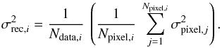${\mathit{\sigma }}_{\mathrm{rec}\mathit{,i}}^{\mathrm{2}}\mathrm{=}\frac{\mathrm{1}}{{\mathit{N}}_{\mathrm{data}\mathit{,i}}}\left(\frac{\mathrm{1}}{{\mathit{N}}_{\mathrm{pixel}\mathit{,i}}}\sum _{\mathit{j}\mathrm{=}\mathrm{1}}^{{\mathit{N}}_{\mathrm{pixel}\mathit{,i}}}{\mathit{\sigma }}_{\mathrm{pixel}\mathit{,j}}^{\mathrm{2}}\right)\mathit{.}$(A.2)

To estimate the turbulent contribution to ${\mathit{\sigma }}_{\mathit{i}}^{\mathrm{2}}$, we adopt a very crude model of interstellar turbulence, which we assume consists of turbulent cells, all of which have the same size l, cause a magnetic field perturbation δB with constant strength and random direction, and produce no perturbation in the free-electron density. The FD associated with an individual turbulent cell can then be written as ${\mathit{\sigma }}_{\mathrm{cell}}\mathrm{=}{\mathit{n}}_{\mathrm{e}}\mathit{\delta }{\mathit{B}}_{\mathrm{\parallel }}\mathit{l,}$(A.3)where n_e is the background free-electron density at the cell’s location (given by Schnitzeler’s 2012 updated version of the NE2001 model, as described in Sect. 4.1) and δB_∥ is the rms line-of-sight component of δB. For an isotropic turbulent magnetic field, $\mathit{\delta }{\mathit{B}}_{\mathrm{\parallel }}\mathrm{=}\mathit{\delta B}\mathit{/}\sqrt{\mathrm{3}}$. Here, we adopt δB = 5 μG (Rand & Kulkarni 1989; Ohno & Shibata 1993) and l = 100 pc (Haverkorn & Spangler 2013, and references therein).

To properly account for the line-of-sight variations of the number and FD of turbulent cells contributing to ${\mathit{\sigma }}_{\mathrm{turb}\mathit{,i}}^{\mathrm{2}}$, we divide the Galactic volume subtended by bin i into N_layer,i successive layers of thickness l. For future reference, if we denote by L_i the effective path length from the observer to the edge of the Galaxy in the direction of bin i, we simply have N_layer,i = L_i/l. We identify each layer by its running number k (starting from k = 1 in the closest layer), and we denote by N_cell,ik the statistical number of turbulent cells in layer k of bin i. As illustrated in Fig. A.1, there is an important difference between distant and nearby layers. A distant layer of bin i encloses several cells, whose contributions to ${\overline{\mathrm{FD}}}_{\mathrm{obs}\mathit{,i}}$ tend to statistically average out over the layer. In contrast, a nearby layer of bin i can be completely filled with a single cell, which then gives a coherent contribution (with no averaging-out) across the layer. Since all the bins have an angular size θ_bin ≃ 10° (see Sect. 2.1), the transition from a single cell to several cells per layer occurs at a line-of-sight distance L_tr = l/θ_bin ≃ 570 pc, i.e., after a number of layers N_near = L_tr/l = 1 /θ_bin ≃ 5.7. Thus, for k ≤ N_near, N_cell,ik = 1, while for k ≥ N_near, N_cell,ik = (θ_bink)² = (k/N_near)².

The contribution from layer k of bin i to ${\mathit{\sigma }}_{\mathrm{turb}\mathit{,i}}^{\mathrm{2}}$ is equal to the mean FD squared of the enclosed turbulent cells divided by the number N_cell,ik of these cells: 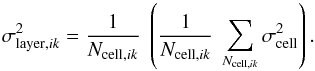${\mathit{\sigma }}_{\mathrm{layer}\mathit{,ik}}^{\mathrm{2}}\mathrm{=}\frac{\mathrm{1}}{{\mathit{N}}_{\mathrm{cell}\mathit{,ik}}}\left(\frac{\mathrm{1}}{{\mathit{N}}_{\mathrm{cell}\mathit{,ik}}}\sum _{{\mathit{N}}_{\mathrm{cell}\mathit{,ik}}}{\mathit{\sigma }}_{\mathrm{cell}}^{\mathrm{2}}\right)\mathit{.}$(A.4)Finally, the uncertainty in ${\overline{\mathrm{FD}}}_{\mathrm{obs}\mathit{,i}}$ due to turbulent fluctuations in the magneto-ionic ISM is the quadratic sum of the contributions from the N_layer,i layers of bin i: 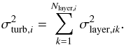${\mathit{\sigma }}_{\mathrm{turb}\mathit{,i}}^{\mathrm{2}}\mathrm{=}\sum _{\mathit{k}\mathrm{=}\mathrm{1}}^{{\mathit{N}}_{\mathrm{layer}\mathit{,i}}}{\mathit{\sigma }}_{\mathrm{layer}\mathit{,ik}}^{\mathrm{2}}\mathit{.}$(A.5)

Let us emphasize that Eq. (A.5) provides only a very rough expression for σ_turb,i, which ignores spatial variations in the turbulence parameters (e.g., in the size and field strength of turbulent cells) as well as correlations between them (e.g., between fluctuations in field strength and in free-electron density). In that respect, we note that spatial variations in the turbulence parameters are partly washed out when summing over all the layers along the line of sight to obtain ${\mathit{\sigma }}_{\mathrm{turb}\mathit{,i}}^{\mathrm{2}}$ (Eq. (A.5)) and when summing over all the bins to obtain χ² (Eq. (39)). There might also be some cancellation, for instance, between δB being larger and l being smaller in spiral arms than in interarm regions (see, e.g., Beck 2009, Haverkorn et al. 2008, respectively) and between δB decreasing (together with B) and l increasing with increasing | z | (Ann Mao, priv. comm.). Incidentally, the variations of δB and l with | z | are probably not too critical, as they are weighted down by a decreasing n_e.

Let us also remark that σ_turb,i is sensitive to the poorly known values of l and δB. To quantify this sensitivity, we write out the full expression of ${\mathit{\sigma }}_{\mathrm{turb}\mathit{,i}}^{\mathrm{2}}$ by inserting Eqs (A.3) into (A.4) and Eqs. (A.4) into (A.5). If we denote by $\mathrm{(}{\mathit{n}}_{\mathrm{e}}^{\mathrm{2}}{\mathrm{)}}_{\mathit{ik}}$ the mean value of ${\mathit{n}}_{\mathrm{e}}^{\mathrm{2}}$ over layer k of bin i and by N′_near the closest integer below N_near (defined above Eq. (A.4)), we readily obtain 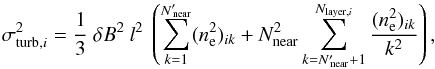${\mathit{\sigma }}_{\mathrm{turb}\mathit{,i}}^{\mathrm{2}}\mathrm{=}\frac{\mathrm{1}}{\mathrm{3}}\mathit{\delta }{\mathit{B}}^{\mathrm{2}}{\mathit{l}}^{\mathrm{2}}\left(\sum _{\mathit{k}\mathrm{=}\mathrm{1}}^{{{\mathit{N}}^{\mathrm{\prime }}}_{\mathrm{near}}}\mathrm{(}{\mathit{n}}_{\mathrm{e}}^{\mathrm{2}}{\mathrm{)}}_{\mathit{ik}}\mathrm{+}{\mathit{N}}_{\mathrm{near}}^{\mathrm{2}}\sum _{\mathit{k}\mathrm{=}{{\mathit{N}}^{\mathrm{\prime }}}_{\mathrm{near}}\mathrm{+}\mathrm{1}}^{{\mathit{N}}_{\mathrm{layer}\mathit{,i}}}\frac{\mathrm{(}{\mathit{n}}_{\mathrm{e}}^{\mathrm{2}}{\mathrm{)}}_{\mathit{ik}}}{{\mathit{k}}^{\mathrm{2}}}\right)\mathit{,}$(A.6)where the first term represents the contribution from the N′_near nearest layers, which contain a single cell (N_cell,ik = 1), and the second term represents the contribution from the N_layer,i−N′_near more distant layers, which contain more than one cell (N_cell,ik = (k/N_near)²). It emerges from Eq. (A.6) that σ_turb,i varies linearly with δB. This is because σ_turb,i depends on δB only through the FD of individual turbulent cells, σ_cell, which is a linear function of δB (see Eq. (A.3)). Variations with l are a little more subtle: in addition to an explicit linear variation similar to that found for δB, there is a more complex implicit variation through $\mathrm{(}{\mathit{n}}_{\mathrm{e}}^{\mathrm{2}}{\mathrm{)}}_{\mathit{ik}}\mathrm{=}\mathrm{(}{\mathit{n}}_{\mathrm{e}}^{\mathrm{2}}{\mathrm{)}}_{\mathit{i}}\mathrm{(}\mathit{s}\mathrm{=}\mathit{k}\hspace{0.17em}\mathit{l}\mathrm{)}$ and N_layer,i = L_i/l. The former arises through σ_cell, which is a linear function of l (see Eq. (A.3)), while the latter results from the way the individual σ_cell combine together to produce a net σ_turb,i. As we now show, the implicit variation with l is actually quite weak. Indeed, our chosen parameter values pertain to the limit L_i ≫ L_tr or, equivalently, N_layer,i ≫ N_near, which has two important consequences. First, the exact value of N_layer,i, which enters Eq. (A.6) only as the upper bound of a rapidly converging series, has hardly any impact. Physically, only the N′_near nearest layers, with a single cell, and the next few layers, with a small number of cells, contribute significantly to σ_turb,i; more distant layers have their contributions increasingly reduced by averaging over an increasing number of cells (prefactor 1 /N_cell,ik in Eq. (A.4), leading to the factor 1 /k² in the second term of Eq. (A.6)). Second, the value of $\mathrm{(}{\mathit{n}}_{\mathrm{e}}^{\mathrm{2}}{\mathrm{)}}_{\mathit{ik}}$ in the first few, significantly-contributing layers is not very different from the local value of ${\mathit{n}}_{\mathrm{e}}^{\mathrm{2}}$, and hence not very sensitive to l. Altogether, σ_turb,i varies a little less than linearly with l.

Plotted in Fig. A.2 is the total uncertainty in ${\overline{\mathrm{FD}}}_{\mathrm{obs}\mathit{,i}}$, σ_i (thick magenta line), for the 356 bins with latitude | b | ≥ 10°, together with the contributions from the reconstruction of Oppermann et al. (2015), σ_rec,i (red line), and from turbulent fluctuations, σ_turb,i (brown line). Also shown are the contributions to σ_turb,i from the N′_near nearest layers, which contain a single turbulent cell (thin green line), and from the N_layer,i−N′_near more distant layers, which contain more than one cell (thin blue line). It appears that, for our choice of parameter values, σ_turb,i is typically one order of magnitude larger than σ_rec,i and σ_turb,i generally has comparable contributions from nearby and distant layers. There is a general tendency for σ_rec,i to decrease with increasing | b | (toward the ends of the x-axis) and a weaker tendency for σ_turb,i to do so above the midplane (in the right half of the figure). In addition, both σ_rec,i and σ_turb,i undergo modulations with longitude, ℓ. The modulation of σ_rec,i, mostly apparent below the midplane (in the left half of the figure), arises from a lack of data points with declination δ< −40°. In contrast, the periodic fluctuations of σ_turb,i, visible at all latitudes, are linked to the spatial (mainly longitudinal) variations of the free-electron density in the local ISM. Finally, the sharp peaks around i = 150 and i = 258 find their origin in strong, localized enhancements in the free-electron density associated with nearby interstellar structures (mainly the Gum nebula and the Vela supernova remnant; see Purcell et al. 2015, and references therein). These peaks hardly affect the results of our analysis: they only reduce the weight of the corresponding bins in the expression of χ² (Eq. (39)).

Appendix B: Impact of the model parameters on the ${\overline{\mathrm{FD}}}_{\mathrm{mod}}$ map

For compactness, the present discussion focuses on the halo-field models, A, B, C, and D (presented in Sect. 3.1), but all our conclusions also hold for the corresponding disk-field models, Ad, Bd, and Dd (presented in Sect. 3.2) – remember that there is no model Cd.

All the field models are expressed in terms of a small number of free parameters, which are related to either the shape of field lines or the field strength distribution. The parameters governing the spiral shape of field lines (p₀, H_p, L_p; see Eq. (23)) are common to all the models; the parameters governing the shape of poloidal field lines (r₁, | z₁ |, a, n; see Eqs. (3), (7), (12), (16)) apply each to one pair of models (A and B, C and D, A and C, B and D, respectively); and the parameters governing the field strength distribution (B₁, H, L, m, ϕ_⋆; see Eqs. (11) and (20)) enter either all the models or only one pair of models (all, A and B, C and D, all, all, respectively). The azimuthal wavenumber, m, stands apart for its discrete values, which we further restricted in Sect. 5.1 to m = 0 (axisymmetric) and m = 1 (bisymmetric). In this appendix, we successively consider these two values, and for each, we discuss the impact of all the other free parameters on the modeled ${\overline{\mathrm{FD}}}_{\mathrm{mod}}$ map, noting that ϕ_⋆ is relevant only when m ≠ 0. Because the discussion of the m = 0 case will serve as a basis for the m = 1 case, we prefer to keep model A in the former, even though the inherent singularity of model A can only be removed in non-axisymmetric configurations (see Sect. 3.1.4).

Appendix B.1: Axisymmetric (m = 0) case

We first consider the parameters governing the field strength distribution: the normalization field strength, B₁ (in Eqs. (11) and (20)), the exponential scale height, H (in Eq. (11) for models A and B), and the exponential scale length, L (in Eq. (20) for models C and D). The effect of B₁ is straightforward. The two poloidal components of the magnetic field (given in Sect. 3.1.1), as well as its azimuthal component (given by Eq. (28)), vary linearly with B₁. The same must hold true for the line-of-sight field component, and hence for the Galactic FD (Eq. (2)). In consequence, B₁ sets the overall amplitude of the ${\overline{\mathrm{FD}}}_{\mathrm{mod}}$ map, with no impact on its detailed structure. H and L, for their parts, control the vertical and radial profiles of the field strength on the reference surface and, by implication, throughout the Galaxy. Small values of H or L entail a rapid fall-off of the field strength with | z | or r, which, in turn, tends to confine the large FD values to low | b | or small ℓ, respectively. Accordingly, the ${\overline{\mathrm{FD}}}_{\mathrm{mod}}$ map tends to be dominated by a band along the Galactic plane (with longitudinal modulation; see next paragraph) or along the prime (ℓ = 0°) meridian, respectively. Larger values of H or L tend to maintain large FD values up to higher | b | or out to larger ℓ, so that the ${\overline{\mathrm{FD}}}_{\mathrm{mod}}$ map tends to show a distribution that is more extended in latitude or in longitude, respectively. It should be emphasized, though, that the effect of H and L is weighted by the free-electron density and, therefore, becomes increasingly weak as H or L grows above the free-electron scale height or scale length, respectively.

We now turn to the parameters governing the spiral shape of field lines, i.e., the parameters involved in the shifted winding function (Eq. (23)): the pitch angle at the origin, p₀, the vertical scale height, H_p, and the radial scale length, L_p. As indicated by Eq. (28), the ratio of azimuthal-to-poloidal field varies with r and z and goes to zero for r → ∞ or | z | → ∞. In the limit p₀ → 0°, the field is purely azimuthal throughout the Galaxy, so that the Galactic FD (Eq. (2)) reverses sign at ℓ = 0°,180° and peaks at intermediate ℓ in the inner Galactic quadrants. The ${\overline{\mathrm{FD}}}_{\mathrm{mod}}$ map is then approximately¹³ antisymmetric with respect to the prime meridian and dominated (in each hemisphere) by two patches of opposite signs on either side of the prime meridian. Conversely, in one of the three limits | p₀ | → 90°, H_p → 0, or L_p → 0, the field is purely poloidal everywhere (except at z = 0, when only H_p → 0), so that the Galactic FD generally peaks around ℓ = 0°, with a secondary peak around ℓ = 180°, and reverses sign at intermediate ℓ. The ${\overline{\mathrm{FD}}}_{\mathrm{mod}}$ map is then approximately¹³ symmetric with respect to the prime meridian and dominated (in each hemisphere) by one patch straddling it. Between these two extremes, an increase in | p₀ | or a decrease in H_p or L_p tends to make the field globally more poloidal, thereby shifting the longitudes of FD reversals from ℓ = 0°,180° toward intermediate ℓ and the longitudes of peak FD from intermediate ℓ toward ℓ = 0° (stronger peak) and ℓ = 180° (weaker peak). While the value of | p₀ | affects the whole sky, the values of H_p and L_p have more limited effects, which are mainly felt at high | b | and large | ℓ |, respectively.

We finish with the parameters governing the shape of poloidal field lines: the reference radius, r₁ (in models A and B), the positive reference height, | z₁ | (in models C and D), the opening parameter of parabolic field lines, a (in Eq. (3) for model A and Eq. (12) for model C), and the power-law index, n (in Eq. (7) for model B and Eq. (16) for model D). In the present study, the reference radius is set to r₁ = 3 kpc (a plausible value for the inner radius of the Galactic disk), and the positive reference height is set to | z₁ | = 0 in model C and | z₁ | = 1.5 kpc (a plausible value for the transition height between the disk and the halo) in model D. The power-law index turns out to have very little impact on the ${\overline{\mathrm{FD}}}_{\mathrm{mod}}$ map up to at least n = 5. This allows us, for the purpose of speeding up the fitting process, to fix n at its smallest acceptable value, i.e., n = 1 in model B, n = 0.5 in model D, n = 2 in model Bd, and n = 0.5 in model Dd. The opening parameter is more critical, as we now discuss along general lines. To simplify the discussion, we focus on one hemisphere, keeping in mind that the situation in the other hemisphere is either the same or opposite according to whether the magnetic field is symmetric or antisymmetric.

• In model A, small values of a imply that the poloidal field is nearly radial and the total field nearly horizontal. The Galactic FD then has a sinusoidal-like variation with ℓ, weighted toward the inner Galaxy and with zero point depending on pitch angle. Accordingly, the ${\overline{\mathrm{FD}}}_{\mathrm{mod}}$ map is dominated by two patches of opposite signs, with the innermost (lower | ℓ |) patch being predominant. For larger values of a, poloidal field lines are curved toward the rotation axis, and their spacing in azimuthal planes increases with increasing r, hence a faster decline in poloidal field strength and (since B_ϕ is linearly related to B_r and B_z; see Eq. (28)) in total field strength. In the ${\overline{\mathrm{FD}}}_{\mathrm{mod}}$ map, the two dominant patches become weaker – especially the outermost patch, which rapidly fades away – and the line of sign reversal between them (where the field is on average perpendicular to the line of sight) moves away from the pole, toward the innermost patch.

• In model C, small values of a imply that the poloidal field is nearly vertical. The associated Galactic FD keeps the same sign throughout the considered hemisphere, but a generally larger FD, which reverses sign across the prime meridian arises from the azimuthal field. Accordingly, the ${\overline{\mathrm{FD}}}_{\mathrm{mod}}$ map has a single-sign background, onto which are superimposed two patches of opposite signs on either side of the prime meridian. For larger values of a, poloidal field lines are curved toward the Galactic plane, and their spacing in azimuthal planes increases with increasing | z |, hence a faster decline in total field strength. In the ${\overline{\mathrm{FD}}}_{\mathrm{mod}}$ map, the two patches can be either enhanced or weakened, and the line of sign reversal between them moves toward the pole.

In both models A and C, the regions where field lines are most affected by a change in a happen to be the regions where the free-electron density is lowest. This automatically places a limit to the influence of a.

Appendix B.2: Bisymmetric (m = 1) case

The bisymmetric case is generally more complex. The parameters governing the field strength poloidal distribution (B₁, H, L) have basically the same impact on the ${\overline{\mathrm{FD}}}_{\mathrm{mod}}$ map as in the axisymmetric case. The other parameters have the same effect on the spiral and poloidal shapes of field lines, but their exact impact on the ${\overline{\mathrm{FD}}}_{\mathrm{mod}}$ map is more difficult to determine, because it now depends in a strong and fine way on a combination between the shifted winding function, g_ϕ (Eq. (23)) and the orientation angle of the azimuthal pattern, ϕ_⋆ (in Eqs. (11) and (20)).

As it turns out, clear predictions can be made only in the limit | p₀ | → 90° (or, almost equivalently, H_p → 0 or L_p → 0), where g_ϕ → 0 and, therefore, the magnetic field is purely poloidal (see Eqs. (27) or (28)). In this limit, if ϕ_⋆ = 0° or 180°, the field azimuthal modulation (given by the cosine factor in Eqs. (11) and (20)) reaches its maximum amplitude in the azimuthal plane through the Sun (ϕ = 0°), i.e., in the plane ℓ = 0°,180°, where the projection factor of the poloidal field onto the line of sight is also maximum. It then follows that the ${\overline{\mathrm{FD}}}_{\mathrm{mod}}$ map resembles that obtained in the axisymmetric case: it is approximately symmetric with respect to the prime meridian, with (in each hemisphere) a dominant patch straddling it and a line of sign reversal on either side of this patch. In addition, FD has nearly the same peak value, but falls off faster than in the axisymmetric case. If ϕ_⋆ = ± 90°, the field azimuthal modulation reaches its maximum amplitude in the azimuthal plane parallel to the plane of the sky (ϕ = ± 90°) and goes through zero in the azimuthal plane through the Sun (ϕ = 0°), so that FD vanishes at ℓ = 0°,180°. FD also vanishes at two intermediate ℓ of opposite signs where the field is on average perpendicular to the line of sight. The ${\overline{\mathrm{FD}}}_{\mathrm{mod}}$ map is then approximately antisymmetric with respect to the prime meridian and composed (in each hemisphere) of four longitudinal sectors of alternating signs. Moreover, the peak FD values are smaller than in the axisymmetric case, because the poloidal field in the plane of maximum amplitude loses a fraction of its strength upon projection onto the line of sight. Intermediate values of ϕ_⋆ lead to asymmetric configurations with two or four lines of sign reversal and with peak FD values smaller than in the axisymmetric case.

When | p₀ | ≠ 90°, the magnetic field has a non-vanishing azimuthal component, which gives field lines a spiral shape. The azimuthal modulation, imposed on the reference surface, is carried along the spiraling field lines, such that the field generally reverses direction one or several times along any given line of sight. These field reversals lead to an overall reduction of the FD values and to a more structured ${\overline{\mathrm{FD}}}_{\mathrm{mod}}$ map, whose details depend sensitively on the exact g_ϕ−ϕ_⋆ combination.

Appendix C: Confidence intervals and correlations

Appendix C.1: Confidence intervals

The different best-fit parameters discussed in Sect. 5.2 are obtained with very different degrees of accuracy (see Table 2). The most-accurately determined parameter is the pitch angle at the origin, p₀, which is obtained to better than ≈± 3° at the 1σ confidence level when the halo field is axisymmetric (model C0) and better than ≈± 1.3° when the halo field is bisymmetric (model C1). At the other extreme, the orientation angle of the azimuthal pattern, ϕ_⋆, for a bisymmetric field is always very poorly constrained: when the halo field is axisymmetric, the 1σ confidence interval of (ϕ_⋆)_disk covers the entire ± 180° range, and when the halo field is bisymmetric, the 1σ confidence intervals of (ϕ_⋆)_disk and (ϕ_⋆)_halo are nearly the same and both ≈ 100°−160°.

The parameters B₁, H, L, and $\sqrt{\mathit{a}}$ are obtained to better than a factor ≈ 2, with two exceptions. First, in the combination C0-Dd1, L_disk approaches the free-electron scale length, L_e ≃ 11 kpc (see Sect. 4.1), such that its 1σ upper confidence limit can only be inferred to be ≫ L_e (for that reason, it is set to ∞ in Table 2) and its 1σ lower confidence limit is also quite uncertain. Second, in C1-Ad1, the 1σ lower confidence limit of $\sqrt{{\mathit{a}}_{\mathrm{disk}}}$ approaches zero, corresponding to purely horizontal field lines.

The scale height of the winding function, H_p, is well constrained as long as H_p4H_e, with an accuracy better than ≈ ± 15% when the halo field is bisymmetric and ≈ ± 25% in C0-Dd1. However, in C0-Ad1 and C0-Bd1, where H_p ≫ H_e, neither the best-fit value nor the 1σ upper limit of H_p can be derived with any accuracy; only an approximate 1σ lower limit can be drawn. Similarly for the scale length of the winding function, L_p: in all the total-field models, L_p ≫ L_e and only an approximate 1σ lower limit can be drawn. This is because, when H_p ≫ H_e or L_p ≫ L_e, the magnetic field inside the free-electron region (where the Galactic FD arises) depends only weakly on the exact value of H_p or L_p, respectively, which, therefore, can hardly be constrained by the ${\overline{\mathrm{FD}}}_{\mathrm{obs}}$ map. As it turns out, this weak dependence on H_p or L_p extends to the whole Galactic region with non-negligible magnetic field, which means that the large uncertainties in H_p or L_p are luckily not critical for our magnetic field models. Thus, we may set H_p or L_p to a somewhat arbitrary value that is large compared to the size of the Galactic magnetic region and yet small compared to the distance to the external intergalactic medium where field lines are supposed to be anchored (see Sect. 3.1.2). For instance, we may let L_p = 50 kpc in all the total-field models and H_p = 20 kpc in C0-Ad1 and C0-Bd1. In the latter models, Eq. (28) then implies that the azimuthal field component is simply given by B_ϕ ≃ cotp₀B_r, i.e., the pitch angle is nearly constant, throughout the magnetic region.

Another issue that should be addressed here concerns the restrictions imposed on the large-scale magnetic field at the Sun, namely, B_⊙ ∈ [1,2] μG and p_⊙ ∈ [−15°,−4°] (see Sect. 4.1). The imposed range of p_⊙ turns out to have no impact on the final results, as the 1σ confidence intervals of p_⊙ in all six total-field models fall well inside the imposed range of [−15°,−4° ]. Note that p_⊙ is always close to p₀: the best-fit values differ by only ≃ 0.7°−0.8° and the histograms look very similar. This is obviously a direct consequence of the large values of L_p. On the other hand, the imposed range of B_⊙ directly affects our results: the 1σ confidence intervals of B_⊙ are clearly cut off either at 2 μG (in models C0-Ad1 and C0-Bd1) or at both 1 μG and 2 μG (in the three models with C1).

Appendix C.2: Correlations

The confidence intervals shown in Table 2 ignore the possible correlations and degeneracies between parameters. To uncover the important correlations, we consider all the parameters two by two, plot the associated 2D marginalized point densities from the second halves of the relevant Markov chains (see Sect. 4.2), visually examine the 2D density plots, and compute the Pearson and Spearman correlation coefficients as indicators of linear and nonlinear relations, respectively.

In all models, we find strong anti-correlations between B₁ and either H (in models Ad1 and Bd1) or L (in models C0, C1, and Dd1), as well as somewhat weaker anti-correlations between p₀ and both H_p and L_p. These conform to the expected anti-correlation between the normalization value and the scale height/length of a governing quantity. We also find strong anti-correlations between (B₁)_disk and p₀, plus, in some models, weaker anti-correlations between (B₁)_halo and p₀. Physically, an increase in p₀, corresponding to a decrease in | p₀ |, entails an increase in | B_ϕ | (especially at low | z | (see Eq. (28)), i.e., in the disk), and hence a global increase in $\mathrm{\left|}{\overline{\mathrm{FD}}}_{\mathrm{mod}}\mathrm{\right|}$ (especially at low | b | (see Eq. (2), with B_∥ having a contribution ∝ cosb from B_ϕ), i.e., mostly through the disk). To recover a good fit to the observational ${\overline{\mathrm{FD}}}_{\mathrm{obs}}$ map, this global increase in $\mathrm{\left|}{\overline{\mathrm{FD}}}_{\mathrm{mod}}\mathrm{\right|}$ must be counterbalanced by a decrease in (B₁)_disk, sometimes accompanied by a decrease in (B₁)_halo.

The correlations between the disk and halo field parameters are generally weak and not necessarily negative (as might naively be expected). This is because the contributions from the disk and halo fields to ${\overline{\mathrm{FD}}}_{\mathrm{mod}}$ generally add up in some regions and cancel out in other regions. There is, however, one notable exception: when the halo field is bisymmetric, the orientation angles (ϕ_⋆)_disk and (ϕ_⋆)_halo are nearly perfectly correlated. This means that the azimuthal patterns of the disk and halo fields have a narrowly-constrained relative orientation, so that they remain locked to each other even as their combined pattern rotates about its best-fit orientation and as the other parameters vary about their best-fit values.

The orientation angle (ϕ_⋆)_disk is also strongly correlated with the parameters of the winding function, p₀, H_p, and L_p. Remember that (ϕ_⋆)_disk gives the orientation of the bisymmetric azimuthal pattern of the disk field at infinity (see Sect. 3.1.2, below Eq. (26)), whereas the ${\overline{\mathrm{FD}}}_{\mathrm{mod}}$ map is most sensitive to its orientation in the nearby outer Galaxy (see north-south symmetry argument in Sect. 2.2). Both orientations are linked through the winding function. Therefore, a change in (ϕ_⋆)_disk can roughly preserve the azimuthal pattern of the disk field in the nearby outer Galaxy if it is offset by appropriate changes in p₀, H_p, L_p. In practice, due to the tight winding of field lines, a small change in p₀ can be sufficient to offset any change in (ϕ_⋆)_disk. This explains the narrow (≲± 3°) and total (± 180°) 1σ confidence intervals of p₀ and (ϕ_⋆)_disk, respectively, when the halo field is axisymmetric. When the halo field is bisymmetric, the ${\overline{\mathrm{FD}}}_{\mathrm{mod}}$ map is also very sensitive to the orientation of its azimuthal pattern in the inner Galaxy, which is linked, through the winding function, to (ϕ_⋆)_halo, which, in turn, is nearly perfectly correlated to (ϕ_⋆)_disk. To maintain a good fit to the ${\overline{\mathrm{FD}}}_{\mathrm{obs}}$ map, a change in (ϕ_⋆)_disk must now roughly preserve the azimuthal patterns of both the disk field in the nearby outer Galaxy and the halo field in the inner Galaxy, which is again possible with appropriate changes in p₀, H_p, L_p, but only over a limited (≈ 100°−160°) interval of (ϕ_⋆)_disk. Accordingly, the 1σ confidence interval of p₀ is narrower (≲± 1.3°) than when the halo field is axisymmetric, and so are the confidence intervals of H_p and L_p. Another consequence of the locking between the azimuthal patterns of the disk and halo fields is that all correlations tend to be tighter when the halo field is bisymmetric.

All Tables

All Figures

Fig. 1 All-sky map, in Aitoff projection, of the observational Galactic Faraday depth, FDobs, as reconstructed by Oppermann et al. (2015). The map is in Galactic coordinates (ℓ,b), centered on the Galactic center (ℓ = 0°,b = 0°), and with longitude ℓ increasing to the left and latitude b increasing upward. Red [blue] regions have positive [negative] FDobs, corresponding to a magnetic field pointing on average toward [away from] the observer. The color intensity scales linearly with the absolute value of FDobs up to | FDobs | = 400 rad m-2 and saturates beyond this value.

In the text

Fig. 2 All-sky map, in Aitoff projection, showing the disposition of the 428 bins covering the celestial sphere, together with their average observational Galactic Faraday depth, before subtraction of the contribution from Wolleben et al.’s (2010) magnetized bubble. Positive [negative] values are plotted with red circles [blue squares], following the same color intensity scale as in Fig. 1. The coordinate system is also the same as in Fig. 1.

In the text

Fig. 3 All-sky maps, in Aitoff projection, showing the disposition of the 356 bins with latitude | b | ≥ 10°, which are retained for the fitting procedure, together with their average observational Galactic Faraday depth, ${\overline{\mathrm{FD}}}_{\mathrm{obs}}$, after subtraction of the contribution from Wolleben et al.’s (2010) magnetized bubble (top panel). Also shown is the decomposition of ${\overline{\mathrm{FD}}}_{\mathrm{obs}}$ into a symmetric part, ${\overline{\mathrm{FD}}}_{\mathrm{obs}\mathit{,}\mathrm{S}}$ (middle panel), and an antisymmetric part, ${\overline{\mathrm{FD}}}_{\mathrm{obs}\mathit{,}\mathrm{A}}$ (bottom panel). The coordinate system and the color code are the same as in Figs. 1 and 2. The grey band along the Galactic plane masks out the 72 bins with |b| < 10°, which are excluded from the fitting.

In the text

References

- Beck, R. 2009, in IAU Symp. 259, eds. K. G. Strassmeier, A. G. Kosovichev, & J. E. Beckman, 3 [Google Scholar]
- Braun, R., Heald, G., & Beck, R. 2010, A&A, 514, A42 [NASA ADS] [CrossRef] [EDP Sciences] [Google Scholar]
- Brentjens, M. A., & de Bruyn, A. G. 2005, A&A, 441, 1217 [NASA ADS] [CrossRef] [EDP Sciences] [Google Scholar]
- Brown, J. C., Haverkorn, M., Gaensler, B. M., et al. 2007, ApJ, 663, 258 [NASA ADS] [CrossRef] [Google Scholar]
- Burn, B. J. 1966, MNRAS, 133, 67 [NASA ADS] [CrossRef] [Google Scholar]
- Cordes, J. M., & Lazio, T. J. W. 2002, ArXiv e-prints [arXiv:arXiv:astro-ph/0207156] [Google Scholar]
- Dumke, M., Krause, M., Wielebinski, R., & Klein, U. 1995, A&A, 302, 691 [NASA ADS] [Google Scholar]
- Ferrière, K., & Schmitt, D. 2000, A&A, 358, 125 [NASA ADS] [Google Scholar]
- Ferrière, K., & Terral, P. 2014, A&A, 561, A100 [NASA ADS] [CrossRef] [EDP Sciences] [Google Scholar]
- Frick, P., Stepanov, R., Shukurov, A., & Sokoloff, D. 2001, MNRAS, 325, 649 [NASA ADS] [CrossRef] [Google Scholar]
- Gaensler, B. M., Madsen, G. J., Chatterjee, S., & Mao, S. A. 2008, PASA, 25, 184 [NASA ADS] [CrossRef] [Google Scholar]
- Gelman, A., & Rubin, D. B. 1992, Statist. Sci., 7, 457 [NASA ADS] [CrossRef] [Google Scholar]
- Han, J. 2002, in Astrophysical Polarized Backgrounds, eds. S. Cecchini, S. Cortiglioni, R. Sault, & C. Sbarra, AIP Conf. Ser., 609, 96 [Google Scholar]
- Han, J. L., & Qiao, G. J. 1994, A&A, 288, 759 [NASA ADS] [Google Scholar]
- Han, J. L., Manchester, R. N., Berkhuijsen, E. M., & Beck, R. 1997, A&A, 322, 98 [NASA ADS] [Google Scholar]
- Han, J. L., Manchester, R. N., & Qiao, G. J. 1999, MNRAS, 306, 371 [NASA ADS] [CrossRef] [Google Scholar]
- Han, J. L., Manchester, R. N., Lyne, A. G., Qiao, G. J., & van Straten, W. 2006, ApJ, 642, 868 [NASA ADS] [CrossRef] [Google Scholar]
- Harvey-Smith, L., Madsen, G. J., & Gaensler, B. M. 2011, ApJ, 736, 83 [NASA ADS] [CrossRef] [Google Scholar]
- Hastings, W. K. 1970, Biometrika, 57, 97 [Google Scholar]
- Haverkorn, M., & Heesen, V. 2012, Space Sci. Rev., 166, 133 [NASA ADS] [CrossRef] [Google Scholar]
- Haverkorn, M., & Spangler, S. R. 2013, Space Sci. Rev., 178, 483 [NASA ADS] [CrossRef] [Google Scholar]
- Haverkorn, M., Brown, J. C., Gaensler, B. M., & McClure-Griffiths, N. M. 2008, ApJ, 680, 362 [NASA ADS] [CrossRef] [Google Scholar]
- Heesen, V., Krause, M., Beck, R., & Dettmar, R.-J. 2009, A&A, 506, 1123 [NASA ADS] [CrossRef] [EDP Sciences] [Google Scholar]
- Heiles, C. 1996, ApJ, 462, 316 [NASA ADS] [CrossRef] [Google Scholar]
- Jaffe, T. R., Leahy, J. P., Banday, A. J., et al. 2010, MNRAS, 401, 1013 [NASA ADS] [CrossRef] [Google Scholar]
- Jansson, R., & Farrar, G. R. 2012a, ApJ, 757, 14 [NASA ADS] [CrossRef] [Google Scholar]
- Jansson, R., & Farrar, G. R. 2012b, ApJ, 761, L11 [NASA ADS] [CrossRef] [Google Scholar]
- Krause, M. 2009, in Rev. Mex. Astron. Astrofis. Conf. Ser., 36, 25 [Google Scholar]
- Krause, M., Wielebinski, R., & Dumke, M. 2006, A&A, 448, 133 [NASA ADS] [CrossRef] [EDP Sciences] [Google Scholar]
- Lallement, R., Snowden, S., Kuntz, K. D., et al. 2016, A&A, 595, A131 [NASA ADS] [CrossRef] [EDP Sciences] [Google Scholar]
- Mao, S. A., Gaensler, B. M., Haverkorn, M., et al. 2010, ApJ, 714, 1170 [NASA ADS] [CrossRef] [Google Scholar]
- Mao, S. A., McClure-Griffiths, N. M., Gaensler, B. M., et al. 2012, ApJ, 755, 21 [NASA ADS] [CrossRef] [Google Scholar]
- Metropolis, N., Rosenbluth, A. W., Rosenbluth, M. N., Teller, A. H., & Teller, E. 1953, J. Chem. Phys., 21, 1087 [NASA ADS] [CrossRef] [Google Scholar]
- Mitra, D., Wielebinski, R., Kramer, M., & Jessner, A. 2003, A&A, 398, 993 [NASA ADS] [CrossRef] [EDP Sciences] [Google Scholar]
- Moss, D., & Sokoloff, D. 2008, A&A, 487, 197 [NASA ADS] [CrossRef] [EDP Sciences] [Google Scholar]
- Moss, D., Sokoloff, D., Beck, R., & Krause, M. 2010, A&A, 512, A61 [NASA ADS] [CrossRef] [EDP Sciences] [Google Scholar]
- Northrop, T. G. 1963, Rev. Geophys. Space Phys., 1, 283 [NASA ADS] [CrossRef] [Google Scholar]
- Ohno, H., & Shibata, S. 1993, MNRAS, 262, 953 [NASA ADS] [Google Scholar]
- Oppermann, N., Junklewitz, H., Greiner, M., et al. 2015, A&A, 575, A118 [NASA ADS] [CrossRef] [EDP Sciences] [Google Scholar]
- Prouza, M., & Šmída, R. 2003, A&A, 410, 1 [NASA ADS] [CrossRef] [EDP Sciences] [Google Scholar]
- Pshirkov, M. S., Tinyakov, P. G., Kronberg, P. P., & Newton-McGee, K. J. 2011, ApJ, 738, 192 [NASA ADS] [CrossRef] [Google Scholar]
- Purcell, C. R., Gaensler, B. M., Sun, X. H., et al. 2015, ApJ, 804, 22 [NASA ADS] [CrossRef] [Google Scholar]
- Rand, R. J., & Kulkarni, S. R. 1989, ApJ, 343, 760 [NASA ADS] [CrossRef] [Google Scholar]
- Rand, R. J., & Lyne, A. G. 1994, MNRAS, 268, 497 [NASA ADS] [CrossRef] [Google Scholar]
- Robert, C. P. 2015, ArXiv e-prints [arXiv:1504.01896] [Google Scholar]
- Roberts, G. O., Gelman, A., & Gilks, W. R. 1997, The Annals of Applied Probability, 7, 110 [Google Scholar]
- Schnitzeler, D. H. F. M. 2012, MNRAS, 427, 664 [NASA ADS] [CrossRef] [Google Scholar]
- Simard-Normandin, M., & Kronberg, P. P. 1980, ApJ, 242, 74 [NASA ADS] [CrossRef] [Google Scholar]
- Sofue, Y. 2015, MNRAS, 447, 3824 [NASA ADS] [CrossRef] [Google Scholar]
- Soida, M. 2005, in The Magnetized Plasma in Galaxy Evolution, Proc. Conf., eds. K. T. Chyzy, K. Otmianowska-Mazur, M. Soida, & R.-J. Dettmar, 185 [Google Scholar]
- Soida, M., Krause, M., Dettmar, R.-J., & Urbanik, M. 2011, A&A, 531, A127 [NASA ADS] [CrossRef] [EDP Sciences] [Google Scholar]
- Stern, D. P. 1966, Space Sci. Rev., 6, 147 [NASA ADS] [CrossRef] [Google Scholar]
- Stil, J. M., Taylor, A. R., & Sunstrum, C. 2011, ApJ, 726, 4 [NASA ADS] [CrossRef] [Google Scholar]
- Sun, X. H., Gaensler, B. M., Carretti, E., et al. 2014, MNRAS, 437, 2936 [NASA ADS] [CrossRef] [Google Scholar]
- Sun, X. H., Landecker, T. L., Gaensler, B. M., et al. 2015, ApJ, 811, 40 [NASA ADS] [CrossRef] [Google Scholar]
- Sun, X.-H., & Reich, W. 2010, Research in Astronomy and Astrophysics, 10, 1287 [NASA ADS] [CrossRef] [Google Scholar]
- Sun, X. H., & Reich, W. 2012, A&A, 543, A127 [NASA ADS] [CrossRef] [EDP Sciences] [Google Scholar]
- Sun, X. H., Reich, W., Waelkens, A., & Enßlin, T. A. 2008, A&A, 477, 573 [NASA ADS] [CrossRef] [EDP Sciences] [Google Scholar]
- Taylor, A. R., Stil, J. M., & Sunstrum, C. 2009, ApJ, 702, 1230 [NASA ADS] [CrossRef] [Google Scholar]
- Tüllmann, R., Dettmar, R.-J., Soida, M., Urbanik, M., & Rossa, J. 2000, A&A, 364, L36 [Google Scholar]
- Wielebinski, R., & Krause, F. 1993, A&ARv, 4, 449 [NASA ADS] [CrossRef] [Google Scholar]
- Wolleben, M., Fletcher, A., Landecker, T. L., et al. 2010, ApJ, 724, L48 [NASA ADS] [CrossRef] [Google Scholar]