| Issue |
A&A
Volume 600, April 2017
|
|
|---|---|---|
| Article Number | A92 | |
| Number of page(s) | 21 | |
| Section | Stellar atmospheres | |
| DOI | https://doi.org/10.1051/0004-6361/201629337 | |
| Published online | 06 April 2017 | |
The adventure of carbon stars
Observations and modeling of a set of C-rich AGB stars⋆
1 University of Vienna, Department of Astrophysics, Türkenschanzstrasse 17, 1180 Vienna, Austria
e-mail: This email address is being protected from spambots. You need JavaScript enabled to view it.
2 Institut d’Astronomie et d’Astrophysique, Université libre de Bruxelles, Boulevard du Triomphe CP 226, 1050 Bruxelles, Belgium
3 Astronomical Observatory of Padova – INAF, Vicolo dell’Osservatorio 5, 35122 Padova, Italy
4 Department of Physics and Astronomy, Division of Astronomy and Space Physics, Uppsala University, Box 516, 75120 Uppsala, Sweden
5 Physikalisches Institut der Universität zu Köln, Zülpicher Str. 77, 50397 Köln, Germany
Received: 18 July 2016
Accepted: 16 January 2017
Abstract
Context. Modeling stellar atmospheres is a complex and intriguing task in modern astronomy. A systematic comparison of models with multi-technique observations is the only efficient way to constrain the models.
Aims. We intend to perform self-consistent modeling of the atmospheres of six carbon-rich AGB stars (R Lep, R Vol, Y Pav, AQ Sgr, U Hya, and X TrA) with the aim of enlarging the knowledge of the dynamic processes occurring in their atmospheres.
Methods. We used VLTI/MIDI interferometric observations, in combination with spectro-photometric data, and compared them with self-consistent, dynamic model atmospheres.
Results. We found that the models can reproduce spectral energy distribution (SED) data well at wavelengths longer than 1 μm, and the interferometric observations between 8 μm and 10 μm. Discrepancies observed at wavelengths shorter than 1 μm in the SED, and longer than 10 μm in the visibilities, could be due to a combination of data- and model-related effects. The models best fitting the Miras are significantly extended, and have a prominent shell-like structure. On the contrary, the models best fitting the non-Miras are more compact, showing lower average mass loss. The mass loss is of episodic or multi-periodic nature but causes the visual amplitudes to be notably larger than the observed ones. A number of stellar parameters were derived from the model fitting: TRoss, LRoss, M, C/O, and Ṁ. Our findings agree well with literature values within the uncertainties. TRoss, and LRoss are also in good agreement with the temperature derived from the angular diameter T(θ(V−K)) and the bolometric luminosity from the SED fitting Lbol, except for AQ Sgr. The possible reasons are discussed in the text. Finally, θRoss and θ(V−K) agree with one another better for the Miras than for the non-Miras targets, which is probably connected to the episodic nature of the latter models. We also located the stars in the H-R diagram, comparing them with evolutionary tracks. We found that the main derived properties (L, Teff, C/O ratios and stellar masses) from the model fitting are in good agreement with TP-AGB evolutionary calculations for carbon stars carried out with the COLIBRI code.
Key words: stars: AGB and post-AGB / stars: atmospheres / stars: mass-loss / stars: carbon / techniques: interferometric / techniques: high angular resolution
Based on observations made with ESO telescopes at La Silla Paranal Observatory under program IDs: 090.D-0410, 086.D-899, 187.D-0924, 081.D-0021, 086.D-0899.
© ESO, 2017
1. Introduction
Stars less massive than ~8 M⊙ and more massive than 0.8M⊙, after moving from the main sequence (MS) through the Red giant phase and past the Horizontal branch, will spend part of their lives on the asymptotic giant branch (AGB).
At the beginning of the AGB, the stars are characterized by a C-O core, surrounded by two nuclear burning layers: the inner composed of He, and the outer of H. Those layers are in turn wrapped by a convective mantle and, further, by an atmosphere consisting of atomic and molecular gas, which is surrounded by a circumstellar envelope of gas and dust.
The third dredge-up is the mechanism responsible for turning the abundance of AGB stars from O-rich into C-enriched (Iben & Renzini 1983). Carbon-rich AGB stars are one of the most influential contributors to the enrichment of the interstellar medium, with dust made of amorphous carbon (amC) and silicon carbide (SiC). In their atmospheres, carbon-bearing molecules, such as C2, C3, C2H2, CN, and HCN, can be found.
The evolution of the stars on the AGB is characterized by cooling, expansion, and growing in brightness, burning the nuclear fuel faster and faster, until the stars begin to pulsate. The pulsation generates shock waves running through the stars’ atmosphere, creating conditions of pressure and temperature suitable for dust formation. The sequence of pulsation and dust formation may drive a wind off the surface of the star into the interstellar space: when the opacity of amorphous carbon dust is high enough, the radiative pressure provides enough momentum to the grains to accelerate them and to drag along the gas by collisions, causing an outflow from the star (e.g., Fleischer et al. 1992; Höfner & Dorfi 1997).
Höfner et al. (2003) describes this scenario with the solution of the coupled equations of hydrodynamics, together with frequency-dependent radiative transfer, including as well the time-dependent formation, growth, and evaporation of dust grains. The dynamic model atmospheres (DARWIN models, Höfner et al. 2016) that come from this code have successfully reproduced observations; for example, line profile variations (Nowotny et al. 2010) and time-dependent spectroscopic data (Gautschy-Loidl et al. 2004; Nowotny et al. 2013) of carbon-rich stars.
In our previous work (Rau et al. 2015), we studied the atmosphere of the C-rich AGB star RU Vir, comparing, in a systematic way, spectroscopic-, photometric- and interferometric data with the grid of DARWIN models from Mattsson et al. (2010) and Eriksson et al. (2014) .
The investigation of AGB stars using a combination of different techniques has been increasing over the last few years, while, to date, only a few interferometric observations of carbon stars have been directly compared with model atmospheres (Ohnaka et al. 2007; Paladini et al. 2011; Cruzalèbes et al. 2013; Klotz et al. 2013; van Belle et al. 2013). From those, only very few have made use of time-dependent self-consistent dynamic models (Sacuto et al. 2011; Rau et al. 2015). As suggested by Höfner et al. (2003), this is the only way to acquire knowledge about the influence of the dynamic processes on the atmospheric structure at different spatial scales.
The purpose of this paper, is to extend our previous study on RU Vir and to investigate the dynamic processes happening in the atmospheres of a set of C-rich AGB stars. To pursue this goal, we compare predictions of DARWIN models, with observations by means of photometry, spectroscopy and interferometry. Long-baseline optical interferometry is an essential tool to study the stratification of the atmosphere, allowing us to scan the regions of molecules and dust formation.
The target objects of this study are the C-rich AGB stars: R Lep, R Vol, Y Pav, AQ Sgr, U Hya, and X TrA, whose observations and parameters are described in Sect. 2.
Section 3 explores the geometry of the targets. Section 4 introduces the self-consistent dynamic model atmospheres used and presents their comparison with the different types of observables. In Sect. 5, we present our results. Section 6 is a discussion of our results, including a comparison with the evolutionary tracks, and we conclude in Sect. 7 with perspectives for future work.
2. Observational data
2.1. The sample of targets
Our sample consists of stars observed with the Very Large Telescope Interferometer (VLTI) of ESO’s Paranal Observatory with the mid-infrared interferometric recombiner (MIDI, Leinert et al. 2003) instrument; showing (1) a SiC feature in the visibility spectrum and (2) no evidence of asymmetry from differential phase (Paladini et al. 2017). The stars can be grouped into Mira variables (R Lep, R Vol), Semi-regular (Y Pav, AQ Sgr, U Hya), and Irregular (X TrA) stars (Samus et al. 2009).
The main parameters of the stars, namely variability class, period, amplitude of variability, distance, and mass-loss rate, are shown in Table 1. For two stars, namely R Vol and U Hya, we are presenting new VLTI/MIDI data observed within the programs 090.D-0410(A) and 086.D-0899(K). For the remaining stars, our data come from archive observations (Paladini et al. 2017).
Main parameters of our target sample, adopted from the literature.
2.2. Photometry
We collected light curves for the V-band (Pojmanski 2002; Henden et al. 2016), and the bands J, H, K, and L (Whitelock et al. 2006; Smith et al. 2004; Le Bertre 1992). A mean value was derived for each filter with amplitudes derived from the variability (see Table B.1 for details). For the filters where no light curves are available (mainly B, R, and I), we averaged values collected from the literature. The errors were calculated as the standard deviation from those values. For the filters with only one value, without any literature associated error, an error of 20% was assumed.
2.3. Interferometry: MIDI data
All the targets of this study have been observed with the Auxiliary Telescopes (ATs) at VLTI. The observations were carried out with MIDI, which provides wavelength-dependent visibilities, photometry, and differential phases in the N-band (λrange = [ 8,13 ]μm).
Details on the data of R Lep, Y Pav, AQ Sgr, and X Tra are given in Paladini et al. (2017), where the reader will also find the uv-coverage and the journal of the observations.
The journal of observations of R Vol and U Hya is available in Tables B.2 and B.3, together with the uv-coverages (Fig. B.4). The calibrators used are listed below the corresponding science observation. The selection criteria for calibrators’ stars described in Klotz et al. (2012a) were applied. The list of calibrators and their main characteristics are in Table 2.
The data reduction was made with software package MIA+EWS (V2.0Jaffe 2004; Ratzka et al. 2007; Leinert et al. 2003). The size of the error bars is based on the calculated error in the visibilities. A conservative error of 10% on the visibilities is assumed in the case of a calculated error <10%. The wavelength-dependent visibilities shown in Figs. 3 and 4 exhibit the typical shape of carbon stars with dust shells containing SiC grains, which manifest their presence in the visibility minimum around ~11.3 μm. The typical drop in the visibility shape between 8 and 9 μm is caused by C2 H2 and HCN molecular opacities.
3. Geometry of the environment
As a first step, the MIDI interferometric data are interpreted with geometric models. To this end, we used the GEM-FIND tool (GEometrical Model Fitting for INterferometric Data of Klotz et al. 2012b) to fit geometrical models to wavelength-dependent visibilities in the N-band, allowing the constraint of the morphology and brightness distribution of an object. The detailed description of the fitting strategy and of the χ2 minimization procedure can be found in Klotz et al. (2012a).
U Hya has only one visibility spectrum available (see uv-coverage in Fig. B.4, right side) therefore only Uniform Disc (UD) and Gaussian models can be applied. By fitting the data, we derived a UD-equivalent diameter at 8 and 12 μm, of θ8 = 23.89 ± 2.54 mas and θ12 = 39.26 ± 2.64 mas, respectively, and Gaussian full width half maximum (FWHM) at 8 and 12 μm of 14.60 ± 1.68 mas and 24.48 ± 1.87 mas, respectively.
Two MIDI data points are available for R Vol (uv-coverage shown in Fig. B.4, left side). The angular diameters derived from the fit are: θ8 = 26.38 ± 0.17 mas and θ12 = 33.45 ± 0.36 mas for a circular UD fit, and θ8 = 17.88 ± 0.36 mas and θ12 = 24.48 ± 0.60 mas for a fit with a circular Gaussian model.
Geometric modeling for the remaining stars in our sample are presented in Paladini et al. (2017). For a discussion and interpretation, we refer the reader to the values published in their Table 4.
4. Dynamic model atmospheres
Calibrator list.
4.1. Overview of the DARWIN models
Our observational data are compared with synthetic observables obtained from the grid of DARWIN models presented in Mattsson et al. (2010) and Eriksson et al. (2014), and model spectra. A detailed description of the modeling approach can be found in Höfner & Dorfi (1997), Höfner (1999), Höfner et al. (2003), and Höfner et al. (2016). Applications to observations are described in Loidl et al. (1999), Gautschy-Loidl et al. (2004), Nowotny et al. (2010), Nowotny et al. (2011), Sacuto et al. (2011), and Rau et al. (2015).
Those models result from solving the system of equations for hydrodynamics and spherically symmetric frequency-dependent radiative transfer, plus equations describing the time-dependent dust formation, growth, and evaporation. The initial structure of the dynamic model is hydrostatic. A “piston” simulates the stellar pulsation, that is, a variable inner boundary below the stellar photosphere. The “method of moments” (Gauger et al. 1990; Gail & Sedlmayr 1988) calculates the dust formation of amorphous carbon.
The main parameters characterizing the DARWIN models are: effective temperature Teff, luminosity L, mass M, carbon-to-oxygen ratio C/O, piston velocity amplitude Δu, and the parameter fL used in the calculations to adjust the luminosity amplitude of the model. The emerging proprieties of the hydrodynamic calculations are the mean degree of condensation, wind velocity, and the mass-loss rate. A set of “time-steps” describe each model, corresponding to the different phases of the stellar pulsation.
The synthetic photometry, synthetic spectra, and synthetic visibilities are computed using the COMA code and the subsequent radiative transfer (Aringer 2000; Aringer et al. 2009). The synthetic photometry is derived integrating the synthetic spectra over the selected filters mentioned in Sect. 2.2. Starting from the radial temperature-density structure at a certain time-step taken from the dynamical calculation, and considering the equilibrium for ionization and molecule formation, all the abundances of the relevant atomic, molecular, and dust species were calculated. The continuous gas opacity and the strengths of atomic and molecular spectral lines are subsequently determined assuming local thermal equilibrium (LTE). The corresponding data, listed in Cristallo et al. (2007) and Aringer et al. (2009), are consistent with the data used for constructing the models.
Summary of the best fitting model for each type of observation: photometry, spectroscopy, and interferometry.
The amount of carbon condensed into amorphous carbon (amC), in g/cm3, as a direct output of the calculations, is taken from the models. amC dust opacity is treated consistently (Rouleau & Martin 1991 in small particle limit (SPL)), and further details on the dust treatment are given in Eriksson et al. (2014). SiC is added artificially a posteriori with COMA. Following Rau et al. (2015) and Sacuto et al. (2011), the percentage of condensed material is distributed as follows: 90% amorphous carbon, using data from Rouleau & Martin (1991), and 10% silicon carbide, based on Pegourie (1988). Some experiments that change this configuration are presented in Sect. 6.
All grain opacities are calculated for the SPL, in order to be consistent with the model spectra from Eriksson et al. (2014), since an inconsistent treatment of grain opacities causes larger errors in the results, than does using the SPL approximation. The assumed temperature of the SiC particles equals that of amC; this is justified, since the overall distribution of the absorption is relatively similar for both species, except for the SiC feature around 11.3 μm. As a consequence, the addition of SiC would also not cause significant changes in the thermal structure of the models. Since the SPL is adopted, the effects of scattering are not included, as they are neglegible in the infrared.
4.2. The fitting procedure
Generating one synthetic visibility profile for each of the approximately 140 000 time-steps of the DARWIN models grid, and for each baseline configuration of our observations, would be extremely time-consuming from a computational point of view. Therefore a simultaneous fitting of the three types of observables was excluded a priori, instead implementing the procedure described as follows.
First, the photometric observations were compared to the synthetic DARWIN models photometry. In the case of R Lep, the spectro-photometric data were also fitted. A χ2 minimization was performed over the available literature photometric data, for each of the 540 models of the grid, with a total of approximately 140 000 time steps. The best fitting photometry model, with a corresponding best fitting-photometry time-step is listed in Table 3.
We would like to note that it is beyond the scope of this paper to model individual phases in terms of photometry and of interferometry. Indeed, the fit of the average observed photometry to the single time-steps of the models was done only with the aim of pre-selecting a model for the subsequent interferometric comparison.
As mentioned above, it is not feasible to calculate the synthetic intensity profiles and visibilities for each of the grid’s 140 000 time-steps. Furthermore, data longwards of 2 μm are usually single epoch (i.e., one observing date) and the data for the shorter wavelengths are often only a small number of measurements and usually from several light cycles. Therefore, the observations correspond to a random mixture of phases, both with respect to wavelength (phase coverage of different filters quite different) and with respect to cycles. Thus, in our case, the mean of the available photometry is different from the mean SED (which corresponds to a mean pulsational phase).
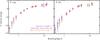 |
Fig. 1 Photometric observations of Mira stars: R Lep (left) and R Vol (right). Observations (violet circles) are compared to the DARWIN model’s synthetic photometry (gray diamonds). Orange diamonds show the best fitting time-steps of the two stars. |
Second we produced the synthetic visibilities, following the approach of Davis et al. (2000), Tango & Davis (2002) and Paladini et al. (2009). They are calculated as the Hankel transformation of the intensity distribution I, which results from the radiative transfer. We then compared them to the interferometric MIDI data of each star. For the time-computational reasons mentioned before, we only produced the synthetic visibilities for all the time-steps belonging to the best fitting photometric model.
Concerning interferometry, no variability in the N-band was observed for the semi-regular star R Scl (Sacuto et al. 2011) and for the irregular star TX Psc (Klotz et al. 2013). Paladini et al. (2017), where a selection of our targets are studied (R Lep, Y Pav, AQ Sgr, and X TrA), concluded that interferometric variability is approximately 10% or even less. Following these results, and considering that 10% is the typical error of our interferometric dataset, we assume that no interferometric variability is present and we combine the observations as representative of one single snapshot of the star. Indeed, if data for more than one epoch are available, then all data will be combined for the fit. Generally, we have MIDI data for only one or two epochs, with typically a small or no overlap in baseline and position angle as would be necessary in order to check for interferometric variability. Therefore, fitting individual data for single epochs with single time steps would have notably reduced the significance of the fits. The sparse coverage in variability phase and uv-space of the MIDI observations also did not indicate a fit of averaged observations with averaged model visibilities. The interferometric χ2 values of the best fitting timesteps (Table 3) are provided for completeness and to guide the discussion. For readability of the figures involving model visibilities, only the best time-step is shown. The assumption of small interferometric variability and the range of model visibilities are discussed in Sect. 5.2.1.
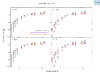 |
Fig. 2 Photometric observations of SRb and Lb stars: Y Pav (upper left) and AQ Sgr (upper right), and U Hya (lower left) and X TrA (lower right). Observations (violet circles) are compared to the DARWIN model’s synthetic photometry (gray diamonds). Orange diamonds show the best fitting time-steps of the four stars. |
In the following paragraphs, we present the results of the comparison of the DARWIN models with the spectrophotometric and interferometric data for each single star. One example of the confrontation of the intensity profile and visibility versus baseline at two different wavelengths, namely 8.5 μm for the molecular contribution and 11.3 μm for the SiC feature, is shown in Fig. 6 (see Appendix for the other stars).
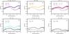 |
Fig. 3 Visibility dispersed over wavelengths of the Mira variables of our sample. Models are plotted in full lines, observations in dashed lines, at the different projected baselines (see color legend). The stars are identified in the title. The six panels show R Lep dispersed visibilities at the baseline configuration D0-A1 a); D0-B2 b); H0-I1 c); and A1-G1 d), as also marked in the plot titles. R Vol dispersed visibilities are at the baseline configuration A1-G1 e) and A1-K0 f). Error bars are of the order of 10%, and a typical error-size bar is shown in gray in each panel, overlapping with the data at 8.5 μm. In panel a), the two models’ full lines are overlapping, as the two observations lines. In panel d), the two lines of the observations are overlapping, and the model at Bp = 79 also lies on top of them. |
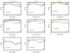 |
Fig. 4 As in Fig. 3, for the semi-regular and irregular stars of our sample: Y Pav in panels a), b), c); X TrA in panels d), e), f); U Hya in panel g) and AQ Sgr in panel f). Error bars are of the order of 10%, and a typical error-size bar is shown in gray in each panel, overlapping with the data at 8.5 μm. Panels c), d), and f) show the two full lines (models) that overlap. |
5. Results
The fits of the DARWINs models with our three different types of observations, lead to results which are described in this section, for Mira, semi-regular, and irregular stars. We refer to Sect. 6 for a detailed discussion of our results.
The results of the fit, namely the χ2, are shown in Table 3. The main parameters that characterize the models, as described in Sect. 4, are listed together with the resulting properties of the DARWIN models, such as the mean mass-loss rate Ṁ. No assignment of MIDI phases can be done for the semi-regular and irregular variables due to the irregular nature and also sometimes poor phase coverage of the light curves. We further note that all our targets show no evidence of asymmetry from differential phase in the MIDI data (see also Paladini et al. 2017).
The best fitting models of Y Pav, AQ Sgr, U Hya, and X TrA resulted, at first, in models without mass loss. Since those stars display mass loss in the literature (see Table 1), we decided to perform a selection a priori, choosing from the whole grid of 560 models, only the ones allowing for wind formation, that is, having a condensation factor fc> 0.2. This results in a sub-grid of 168 models, among which we performed our analysis for the semi-regular and irregular stars. We also discuss the fits with the windless models for these stars in Sect. 5.2.
Based on our findings, some general statements can be made. Overall, the χ2 from SED fitting of non-Miras is higher than that obtained for Mira variables (Table 3). We also found that the Miras interferometric observations show the SiC feature as being shallower than that produced by the DARWIN models.
5.1. Mira stars
The spectroscopic and photometric data of R Lep agree well with the model predictions, as can be seen in Fig. 5 (in which the IRAS spectrum has been over-plotted for qualitative comparison) and Fig. 1, left panel. The small differences at wavelengths shorter than 1 μm are discussed later in Sect. 6.1.1. The model SED shows an emission bump around 14 μm, which is not seen in the observed spectrum, as also noticed by Rau et al. (2015). The origin of this feature predicted by the model, is due to C2H2 and HCN, as mentioned by Loidl (2001), and discussed in Sect 6.1.2.
The good fit is confirmed by a χ2 of 0.99 and 1.01 for photometry and interferometry, respectively (Table 3). R Lep interferometric data are shown in Figs. 6 and 3 (upper panels). In the latter, the typical SiC shape around 11.3 μm is visible. This shape is reproduced by the models, and their difference in visibility level at wavelengths longer than 10 μm will be discussed in Sect. 6.
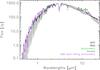 |
Fig. 5 Observational spectro-photometric data of R Lep, compared with the synthetic spectrum of the best-fitting time-step (violet). Photometry is plotted in green circles, while IRAS (Olnon et al. 1986) and NASA/IRTF (Rayner et al. 2009) spectra are plotted as black lines to allow qualitative verification of the photometric fit. The spectrum of the DARWIN models, for which the synthetic photometry fits best the corresponding observational data, is shown in violet. |
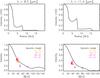 |
Fig. 6 Interferometric observational MIDI data of R Lep, compared with the synthetic visibilities based on the DARWIN models; top: intensity profile at two different wavelengths: 8.5 μm and 11.4 μm and bottom: visibility versus baseline; the black line shows the dynamic model and the colored symbols illustrate the MIDI measurements at different baselines configurations. |
The R Vol photometric data show good agreement at all wavelength ranges, well within the error bars (see Fig. 1, right panel). The interferometric data of R Vol are taken with long baselines (Bp = 74 m and Bp = 126 m), and cover visibility values between 0.05 and 0.15. Overall, the observations taken with the 126 m baseline (Fig. 3) are reproduced by the model in the wavelength range between 11 and 13 μm. However, the model predicts higher visibilities for the 74 m baseline.
In summary, the Mira stars exhibit a visibility versus wavelength profile that is always flatter than the models, and agrees better at wavelengths shorter than 10 μm. A similar finding was reported by Sacuto et al. (2011) for R Scl.
5.2. Semi-regular and irregular variables
As mentioned above, at first, the best fitting models of semi-regular and irregular stars resulted in those without mass-loss. The corresponding classes resulted in pp (periodically pulsating) for Y Pav, U Hya and X TrA, and pn (non-periodic) for AQ Sgr. The parameters of those models without mass loss are indicated in Table 3 for comparison. In general, the χ2 of the photometry of the semi-regular and irregular stars is higher than for the Miras (see Table 3). Compared to the windless models, the fit of SEDs with mass-losing models (fc > 0.2) did not lead to a better fit for wavelengths shorter than 1 μm. Furthermore, the total visual amplitudes of these models, which are mostly due to variable dust extinction (Nowotny et al. 2011) are markedly larger than the observed ones. On the other hand, all these models have either episodic or multi-periodic mass loss which leads to less regular or multi-periodic synthetic light curves, similar to the observed characteristics. Looking at individual cycles, the visual amplitudes are closer to the observed ones. The visibility slope of the models with mass loss agrees better than for Miras, and the visibility level is always high, except for U Hya (for detailed plots please refer to Figs. 7, B.1, B.2, and B.3). We would like to underline that in comparison, the windless models are too compact and also lack the SiC signatures observed in the visibilities. This can be seen in Figs. A.1 and A.2, that show visibilities versus wavelength for the best-fitting models without mass loss for Y Pav (semi-regular) and X TrA (irregular), respectively. We thus decided, based on the observed mass loss and the significantly better fit of the visibilities, to consider the mass-losing models for the remaining analysis.
The synthetic SED from the DARWIN models of Y Pav agrees with the observations well, except for the B filter (see Fig. 2). The problem of having the B filter photometric data off the fit, also appearing for some of the other targets, also manifests itself in the SED of Y Pav, and a likely reason of this is discussed in Sect. 6. The interferometric data show a high visibility level at all three Y Pav baseline configurations. The models agree in level with the MIDI observations, and their difference in shape is discussed in Sect. 6.
The synthetic photometry of AQ Sgr fits the data well within the error bars. The absolute visibility level of the MIDI data is in agreement with the models, but the SiC feature shape is not as pronounced in the models as in the observations.
The synthetic DARWIN models’ SED of U Hya is in good agreement with the observations. The small discrepancy shorter than 1 μm is discussed in Sect. 6. The synthetic visibilities seem to reproduce the shape and level of the MIDI U Hya observations well, and within the error bars.
Since at first the photometry of X TrA in Fig. 2, lower right panel, had the value in the filter I particularly offset compared to the overall fit, we performed a new fit excluding those values. Since the “new” best fitting model has no mass loss, we repeated the fitting procedure again following the selection of models explained in Sect. 4.2. The reduced χ2 obtained for the SEDs following this procedure is equal to 6.2. The results are shown in Table 3 and Fig. 2. There is a good agreement between models and MIDI observations, and the discrepancy in shape is examined in Sect. 6.
5.2.1. Interferometric variability
The data of Y Pav, U Hya, and AQ Sgr have been taken at single epochs, therefore no interferometric variability can be assessed for those stars. The observations of R Vol are one year apart, but very different in projected baseline (Bp) and projected angles (PA), a configuration that makes the variability check impossible to perform. The X TrA observations are numerous and taken at the same time, but they are different in PA, thus the time-variability can also not be evaluated.
The only target for which a variability check could be performed is the Mira star R Lep. For this check, the two R Lep datasets at Bp = 40 m can be used. A small variation in the visibility level is noticeble between 9 μm and 10 μm (see Fig. 3, panel c). The highest difference in visibility level is found at 9.7 μm, where the variation of visibility is δV = 0.072, which is barely significant compared to the typical errors of ~10% (see Fig. 12 for an example of the typical errors on the observed visibilities). The visibility level decreases when moving from pre-minimum (φ = 1.43 at Bp = 40, PA = 147) to post-minimum (φ = 0.66 at Bp = 40, PA = 142). This behavior goes in the same direction as the one found in the study of the Mira star V Oph by Ohnaka et al. (2007). Indeed, they observed the star to be smaller close to the minimum of the visual phase, with a variation in the visibility level: δV = 0.25 between datasets #3 (phase φ = 0.49) and #6 (φ = 0.69) at 8.3, 10.0, and 12.5 μm – see Fig. 2 in Ohnaka et al. 2007. The spatial frequency of the R Lep measurements is smaller than that of the V Oph data and gets even smaller when considering the smaller distance of V Oph (237 pc, van Leeuwen 2007). As can be seen from Fig. 2 of Ohnaka et al. (2007), the variability decreases with decreasing spatial frequency. However, the lower visibilities found for R Lep at all spatial frequencies indicate a significantly different structure when compared to V Oph, probably in the sense of an overall larger extension of R Lep. Thus a comparison of these two stars is difficult.
The above mentioned datasets do not only have a different variability phase but also belong to different cycles. Since the projected baselines and projected angles are similar, we used these data to check our approach of a combined fit of all data with individual times steps. An independent fit of those two observations to our models has been performed, leading to the same best fitting time-step. This result can be understood considering the temporal changes in the predicted visibilities.
Examples of these predicted changes in the visibilities are shown in Figs. 8–10 for the best fitting model of R Lep. For both Miras, the observed visibilities are at or close to the lower envelope of the predicted visibilities for all the time steps of the best fitting model. For the non-Miras, the observations fall within the range of predicted visibilities and this range is larger than the one of the models for the Miras. The latter result is caused by cycle-to-cycle variation of the models; within each cycle, the ranges are comparable. If our assumption of a small interferometric variability is correct, then the models for the Miras would predict an overly large variability and would be too compact on average. If the real variability is not small, we cannot draw any conclusion on the agreement between observed and predicted variations, since the phase and uv-coverage of the MIDI observations is too small. Concerning the wavelength dependence of the visibilities, we note that the overall shape of the visibilities dispersed in wavelength is very similar from time step to time step, the major difference being in the overall level of visibility. This is important to keep in mind for the discussion in Sects. 6.1.2 and 6.1.3.
6. Discussion
6.1. The SEDs and visibilities
Our attempts to reproduce the SED (photometry + IRTF spectrum in the R Lep case) and interferometric MIDI data with DARWIN models show a strong improvement with respect to our previous study of RU Vir. The models can reproduce the SEDs of all stars longward of 1 μm relatively well and also the visibilities between 8 μm and 10 μm. In the Miras visibility versus baselines profiles, the observations show a faster decline, leveling off at longer baselines, in comparison to the non-Miras. This behavior is also predicted by the models that are significantly more extended for the Miras and have a more pronounced shell-like structure. This can be most clearly seen by comparing R Lep and Y Pav (Figs. 6 and 7). Indeed, since those two stars are located at very similar distances (see Table 1), the same baselines sample the same spatial frequencies in AU-1. This is also supported by the fact that the best-fitting models (with wind) for the non-Miras have a lower average mass-loss rate and show only episodic mass loss. We remind the reader that, in fact, the best fitting models for the non-Miras were those without a wind and that we excluded those because of the known mass loss for these stars (Sect. 4). Both the windless and episodic models are characterized by relatively compact atmospheres and weakly pronounced gas and dust shells.
In spite of these encouraging results in reproducing the observations, some notable (and partly systematic) differences remain. Therefore, our discussion focuses on three major parts: (1) differences at wavelengths shorter than 1 μm; (2) differences in the visibilities longward of 10 μm and (3) differences related to SiC dust.
6.1.1. Differences at wavelengths shorter than 1 μm
For all the stars in our sample, we noticed some differences at wavelengths shorter than 1 μm. In particular, the difference in the SED fit at the short wavelengths, appearing in Figs. 1 and 2, could be caused by a possible combination of data-related and model-related effects. The data-related ones are due to the stars’ variability, that is, lack of light curves, especially in B, R, and I and partly in the IR.
Concerning semi-regular and irregular stars, their best fitting models are episodic models, as mentioned above, and thus show no regular light curve behavior. These two effects in combination introduce a larger uncertainty in the determination of mean magnitudes for the observations and models and are also responsible for the higher χ2 of the SED fits for non-Miras in comparison with the Miras. Deviations may also be due to the assumption of SPL in the models or uncertainties of the used data set for amC (Nanni et al. 2016).
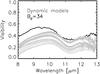 |
Fig. 8 Visibilities dispersed in wavelengths for the shorter baseline (Bp = 34 m) of R Lep observations, in black. The gray lines illustrate the range in visibility of the model’s time-steps. |
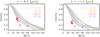 |
Fig. 10 Visibilities vs. baselines of R Lep model, illustrating the range of available synthetic time-steps (in gray) at two chosen wavelengths: 8.5 μm and 11.4 μm. The colored squares are the R Lep observations. |
6.1.2. Differences in the visibilities longwards of 10 μm
Comparing the wavelength dependence of the visibilities for the Miras and the non-Miras with the models (see in Figs. 3 and 4), and ignoring for the moment the differences in the SiC feature, which are discussed in the next section, one notices that at shorter baselines, the Mira models show an increase of visibility with wavelength that is not observed (full lines for the models, and the dashed lines for the observations, respectively). A similar difference was also noticed by us for RU Vir. In Rau et al. (2015), two explanations for this were discussed: (i) a smoother density distribution than in the models and (ii) a clumpy environment. A smoother density distribution with less pronounced dust shells seems possible as the models for the non-Miras do not show this slope in the wavelength-dependent visibilities, and these models generally have weakly pronounced shells (see Figs. 7, B.1, B.2, B.3). A clumpy environment cannot be ruled out, but from our MIDI data, we do not have any evidence of deviations from spherical symmetry; in particular, all the differential phases are not significantly different from zero (see Paladini et al. 2017). Furthermore, the slope of the wavelength-dependent model visibilities agrees relatively well with the observations at the long baselines, where clumps should be more prominent.
In this work, we extended our search to other possible origins of the slope in the models. Using different opacity laws for amC (Zubko et al. 1996; Jager et al. 1998) did not change the slope. Also, changing the distance within the expected uncertainties did not lead to a better agreement.
The DARWIN models are known to poorly reproduce the SED around the 14 μm feature of C2H2 and HCN, mostly due to uncertain opacity and chemistry data (Gautschy-Loidl et al. 2004). We checked the possible influence on the visibilities by artificially removing the C2H2 and HCN contributions from the opacity in the outer parts of the model, this experiment too did not affect the slope. Thus, a smoother density distribution than the one produced by the models is the most likely explanation for the slope difference in the Mira models. Such a smoother density distribution could be caused by less pronounced shocks, which might result from a different cooling function or different dust formation parameters. Further investigation is needed on this matter.
Except for U Hya, all the non-Miras show high visibility levels but no increase with wavelength. The differences to the models are partly related to SiC (see below). For Y Pav, they could also be due to calibration problems at the longest wavelengths (Paladini et al. 2017). The high visibility levels also reduce the sensitivity to the differences in the model parameters because at high visibility, the difference between different time-steps and different models becomes small. Indeed, the objects are only marginally resolved and therefore the observed MIDI data could not significantly constrain the models.
6.1.3. Differences related to SiC dust
Lacking a consistent description of SiC formation in the models, the spectra and visibilities were calculated from the DARWIN models with the assumption that SiC condenses together with amorphous carbon (see Sect. 4). This means that the amount of SiC is proportional to the amount of amC grains and SPL is adopted. This assumption did not lead to major inconsistencies with the observations and is also not in disagreement with theoretical studies on SiC formation. These studies arrive at conflicting results for the condensation sequence of amC and SiC dust. Gail & Sedlmayr (2013) favor the scenario that amC dust condenses before SiC in the case of a stationary wind model. On the other hand, in the models of Ferrarotti & Gail (2006), SiC dust is the first dust component to start growing, which is also supported by the work of Cherchneff (2012). Using models most comparable to our case, Yasuda & Kozasa (2012) find that in the more likely case of non-LTE, the formation region of the SiC grains is more internal and/or almost identical to that of the carbon grains, a scenario also partially favored by Lagadec et al. (2007). A verification of this result requires the implementation of SiC condensation in the DARWIN models in a similar way as currently done for M-type stars (Höfner et al. 2016). This will be the subject of future work.
In this context, we would like to underline that the visibility level, lower inside the SiC feature than around it, must not to be interpreted as a larger extension of SiC with respect to amC and the molecular gas. This conclusion is only true for simple intensity profiles, while our stars have rather complex profiles and the contrast between the different shells containing dust and gas contributes to the influence on the level of visibility. This is illustrated in the comparison of the synthetic intensity and visibility profiles at 8.5 μm and 11.4 μm in Fig. 6. The lower visibility level around 11.3 μm is solely due to the higher SiC opacity with respect to the one of amC.
Whenever the MIDI observations show a clear SiC dust feature, this 11.3 μm SiC feature in the models is more peaked and narrower with respect to the observed one (see R Lep and R Vol in Fig. 3 and U Hya in Fig. 4). A similar effect was noted for RU Vir, both for the spectra and the visibilities. For RU Vir, the spectral fit with hydrostatic models and More Of Dusty (MOD) could be improved by using the distribution of hollow spheres (Groenewegen 2012; Rau et al. 2015). However, this distribution is not yet available for the DARWIN models, and thus it could not be tested.
Another free parameter for the fits is the fraction of Si condensed onto SiC. As explained in Sect. 4, we generally adopted a fraction of 10 %. Increasing this fraction to up to 50 % slightly improves the agreement for R Lep. Also, Y Pav shows some improvements (see Figs. 11 and 12), although for the latter star, the shape of the observed wavelength dependent visibilities is quite different and might not be due to SiC at all. Given the still artificial treatment of SiC in the current models (see Sect. 4), understanding the behaviour of the SiC feature in the model visibilities must await the above-mentioned full implementation of SiC into the DARWIN models.
X TrA is the only star for which no satisfactory fit of the wavelength dependent visibilities could be found. The shape of the model visibility versus wavelength shows almost no SiC, while this is relatively prominent in the data. Scaling the distance and increasing the SiC fraction did not remove this discrepancy. Also, we checked the two models closest in χ2 to the best fitting model (i.e., within 68% of confidence level), in which the predicted SiC feature improves slightly, but the increase with wavelength is too steep, as in the case of Miras. The star is thus compact but apparently has a significant mass-loss. This combination cannot be reproduced by any of the models, and is probably caused by the fact that the star is located in the parameter region of the models with episodic mass loss.
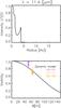 |
Fig. 11 Interferometric observational MIDI data of Y Pav, in cases where the amount of SiC increased to 50% in the models, compared with the synthetic visibilities based on the DARWIN models; top: intensity profile at 11.3 μm and bottom: visibility vs. baseline. The black line shows the dynamic model, the colored symbols illustrate the MIDI measurements at different baseline configurations. |
Observed and calculated temperatures and diameters.
6.2. Fundamental stellar parameters compared to the literature and evolutionary tracks
The best-fitting DARWIN models yield a number of parameters as listed in Table 3.
For a comparison of temperature and luminosity with values found in the literature, we did not use the values given in the table as these refer to the hydrostatic initial model and thus not to the dynamic structure of the model at the time-step (i.e., phase) best fitting the interferometric data (see also Nowotny et al. 2005). Instead, for these time-steps, we calculated a Rosseland diameter (θRoss). The temperature of the time-step at this radius (TRoss) is the corresponding effective temperature, that is, the temperature at the Rosseland radius, defined by the distance from the center of the star to the layer at which the Rosseland optical depth equals 2/3. From this and θRoss, the luminosity LRoss is calculated. From the photometry of our stars, we also derive the bolometric luminosity Lbol, a diameter θ(V−K) using the diameter/(V−K) relation of van Belle et al. (2013), and an effective temperature T(θ(V−K)). The error on the luminosity is assumed to be approximately 40%, on the basis of the distance uncertainty. The errors of the temperature are estimated through the standard propagation of error.
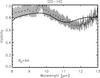 |
Fig. 12 Y Pav wavelength dependent visibilities in the MIDI range, for the only baseline configuration D0-H0, in cases where the amount of SiC increased to 50% in the models. |
The above various resulting stellar parameters are listed in Table 4 together with diameters at 8 μm and 12 μm from geometrical models (see Sect. 3). In Fig. 13, the temperatures and luminosities are compared to thermally-pulsing (TP) AGB evolutionary tracks from Marigo et al. (2013). Starting from the first thermal pulse, extracted from the PARSEC database of stellar tracks (Bressan et al. 2012), the TP-AGB phase is computed until the whole envelope is removed by stellar winds. The TP-AGB sequences are selected with an initial scaled-solar chemical composition: the mass fraction of metals Z is 0.014, and of helium Y is 0.273. In order to guarantee the full consistency of the envelope structure with the surface chemical abundances, which may significantly vary due to the third dredge-up episodes and hot-bottom burning, the TP-AGB tracks are based on numerical integrations of complete envelope models in which, for the first time, molecular chemistry and gas opacities are computed on-the-fly with the ÆSOPUS code (Marigo & Aringer 2009). The results are shown in Fig. 13, where the TP-AGB tracks for two choices of the initial mass on the TP-AGB, M = 1.0 M⊙, and M = 2M⊙, are compared with the stars considered in this work.
We note that the TP-AGB model for M = 1.0M⊙ does not experience the third dredge-up, hence remains with C/O < 1 until the end of its evolution. Conversely, the model with M = 2M⊙ suffers a few third dredge-up episodes that lead to reach C/O > 1, thus causing the transition to the C-star domain. The location of the observed C-stars in the H-R diagram, as well as their C/O ratios, appear to be nicely consistent with the part of the TP-AGB track that corresponds to the C-rich evolution. It is worth noting that the current mass along the TP-AGB track is reduced during the last thermal pulses, which supports (within the uncertainties) the relatively low values of the mass (~0.75−1.0 M⊙) assigned to some stars through the best fitting search on the DARWIN models datset.
Except for Y Pav, the model luminosities and temperatures place the stars in the C-rich domain of the tracks. The model masses are all 1 M⊙ or less except for X TrA. Such low current masses are in agreement with the tracks if the stars are in an advanced stage of the TP-AGB (when log (L) > 3.8). This seems plausible for the Miras but not for the non-Miras. We note that Hinkle et al. (2016) also found C-star masses of between 1 M⊙ and 1.5M⊙. One should however keep in mind the uncertainties in the masses derived from the DARWIN models, and the ones predicted by the tracks.
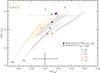 |
Fig. 13 AGB region of the H-R diagram. The lines display solar metallicity evolutionary tracks from Marigo et al. (2013): gray lines mark the regions of Oxygen-rich stars with C/O < 1.0; yellow lines denote the region of C-rich stars with |

The differences between the luminosity and temperature estimations derived from the models (LRoss, TRoss) and the observations (Lbol, T(θ(V−K)) are well within the error bars. Only for AQ Sgr does the difference in luminosity exceed the error. This may be related to the above mentioned episodic mass-loss of the best-fitting model. Literature values of luminosities can be found for three stars in McDonald et al. (2012) and they all agree within the uncertainties, considering the differences in the used data sets and the methods used. We highlight the suprisingly good agreement between TRoss and the purely empirically determined T(θ(V−K)).
Temperature estimates in the literature are all based on fitting photometry with a combination of black bodies or spectra from hydrostatic model atmospheres and a dust envelope around it (Lorenz-Martins et al. 2001; Bergeat & Chevallier 2005; McDonald et al. 2012). For each star, different estimates typically differ by several hundred degrees and our values are always within the range of literature values. For R Vol, only one determination is found in the literature (Lorenz-Martins et al. 2001), which gives a temperature 900 K lower than our TRoss. This apparently large difference can be understood by the method used in Lorenz-Martins et al. (2001), which cannot take into account the very non-static character of a Mira variable and the strong radial overlap of photosphere and dusty envelope in C-rich atmospheres (for a detailed discussion on the concept of an effective temperature for these stars, see also Sect. 3 of Nowotny et al. 2005).
The diameters θRoss and θ(V−K) agree very well for the Miras, while the differences are larger for the non-Miras. This is probably again caused by the structure of models with episodic mass loss. Only R Lep, U Hya, and AQ Sgr have available observed K-diameters (see Table 4). The values agree only approximately and there is no clear systematics in the differences between the three types of parameter. This can be understood by the fact that the three types of diameter sample quite different wavelength ranges and thus are affected quite differently by the non-hydrostatic atmospheric structure and the associated different molecular opacity contributions.
The mass-loss values of the best fitting DARWIN models of the Miras are in reasonable agreement with the literature (see Table 1), while for the non-Miras, we find large differences for AQ Sgr and X TrA. Again, the episodic mass loss of the models is the probable cause.
7. Conclusions
In this work, we present a study of the atmospheres of a set of C-rich AGB stars, combining photometric and interferometric observations, comparing them consistently with a grid of dynamic model atmospheres.
Overall, we found that the fit of DARWIN models’ SEDs with the photometric and interferometric observations presented in this work show a strong improvement with respect to those of RU Vir. The best agreement is found for Mira stars, while for non-Miras the mass-losing DARWIN models have more difficulties in reproducing the photometric observations and amplitudes at wavelengths shorter than 1 μm.
This could be related to the stars variability, since the photometric data in that wavelength region come from various studies. Therefore, a difference in phase is likely. With respect to our previous work on RU Vir, we notice a slight improvement in the agreement of the interferometric data with the models in terms of the level of the visibility versus wavelength, but the difference in shape still remains and is probably due to the amount of condensed dust included in the models, as the experiments mentioned in Sect. 6 prove. Also, the observations show a consistency with the model assumption that SiC and amC condense together.
From our interferometric analysis, it resulted that the models for Miras appear to have a steeper slope in the visibility dispersed in wavelengths, with respect to the observed ones, and a larger extension, with respect to the models for non-Miras. The mass-losing models for the non-Miras do not show this slope of increasing visibility with the wavelengths, generally have weakly pronounced shells, and provide significantly better fits than the windless models.
Due to the sparse phase- and uv-coverage of the MIDI observations, no conclusion can be drawn concerning the agreement between observed and predicted temporal variation in visibility.
We derived stellar parameters through the comparison of photometric and interferometric observations with dynamic model atmospheres and geometric models. Those parameters are summarized in Tables 3 and 4. In the latter, errors on the temperatures are of the order of ±400 K and those on the luminosity are of the order of 2000 L⊙.
Models without the small particle limit assumption have lower condensation degrees, which probably implies less dust extinction in the visual region. Those models will represent a good test to verify the visual excess shown by some of the stars analyzed in this study. Indeed, exclusion of the SPL assumption in a dust shell changes the mid-IR interferometric shape and the temperature-structure. Indeed Mattsson & Höfner (2011) have already studied how, for certain cases, the effect of grain-size dependent opacities can be quite important, especially when strong dust-driven winds do not form in the SPL case, that is, for models near the limit of windless solutions. These might be of special relevance for the semi-regular variables in our sample. Thus, models without the SPL assumption, compared with our observations, will be tested in a follow-up of this work (Rau et al. in prep). Another important aspect that is the subject of ongoing study is the development of mass loss in mildly or irregularly pulsating stars (e.g., Liljegren et al. 2016). While the fits of the mass-losing models for the semi-regular and irregular stars are reasonable for the SEDs and visibilities, the visual amplitudes cannot be reproduced. It is, however, interesting that these models are all episodic or multi-periodic and thus do not have simple periodic light-curves as in the case of Miras.
The second generation VLTI instrument MATISSE (Lopez et al. 2006) will allow imaging at the highest angular resolution. It will therefore be a perfect tool to better reconstruct the intensity profiles of the objects in this study, and to investigate the small-scale asymmetries in order to confirm or deny the asymmetric nature of the objects studied in this work. Also, MATISSE will also help to improve the variability study of those stars and the global distribution of molecules and dust.
Additional interferometric observations of those targets will also help us to better constrain the models. For example, VLTI/PIONIER (H-band, Le Bouquin et al. 2011), GRAVITY (K-band, Eisenhauer et al. 2008), or millimeter/submillimeter interferometric measurements, such as ALMA measurements and VISIR observations, could provide further constraints to solve the open questions.
Available at http://www.jmmc.fr/aspro
Acknowledgments
We thank the anonymous referee for the constructive comments which helped to improve the quality of this paper. This work is supported by the “Abschlussstipendium fellowship” of the University of Vienna, which G.R. thanks, and by the FWF project P23006. P.M. and B.A. acknowledge the support from the ERC Consolidator Grant funding scheme (project STARKEY, G.A. No. 615604). CP is supported by Belgian Fund for Scientific Research F.R.S.- FNRS. We thank the ESO Paranal team for supporting our VLTI/MIDI observations. We thank Thomas Lebzelter for the helpful discussions. This research has made use of the Jean-Marie Mariotti Center Aspro service1 and of SIMBAD database, operated at CDS, Strasbourg, France, and NASA/IPAC Infrared Science Archive.
References
- Aringer, B. 2000, in The Carbon Star Phenomenon, ed. R. F. Wing, IAU Symp., 177, 519 [Google Scholar]
- Aringer, B., Girardi, L., Nowotny, W., Marigo, P., & Lederer, M. T. 2009, A&A, 503, 913 [NASA ADS] [CrossRef] [EDP Sciences] [Google Scholar]
- Bergeat, J., & Chevallier, L. 2005, A&A, 429, 235 [NASA ADS] [CrossRef] [EDP Sciences] [Google Scholar]
- Bressan, A., Marigo, P., Girardi, L., et al. 2012, MNRAS, 427, 127 [NASA ADS] [CrossRef] [Google Scholar]
- Cherchneff, I. 2012, A&A, 545, A12 [NASA ADS] [CrossRef] [EDP Sciences] [Google Scholar]
- Cristallo, S., Straniero, O., Lederer, M. T., & Aringer, B. 2007, ApJ, 667, 489 [NASA ADS] [CrossRef] [Google Scholar]
- Cruzalèbes, P., Jorissen, A., Rabbia, Y., et al. 2013, MNRAS, 434, 437 [NASA ADS] [CrossRef] [Google Scholar]
- Davis, J., Tango, W. J., & Booth, A. J. 2000, MNRAS, 318, 387 [NASA ADS] [CrossRef] [Google Scholar]
- Eisenhauer, F., Perrin, G., Straubmeier, C., et al. 2008, in A Giant Step: from Milli- to Micro-arcsecond Astrometry, eds. W. J. Jin, I. Platais, & M. A. C. Perryman, IAU Symp., 248, 100 [Google Scholar]
- Eriksson, K., Nowotny, W., Höfner, S., Aringer, B., & Wachter, A. 2014, A&A, 566, A95 [NASA ADS] [CrossRef] [EDP Sciences] [Google Scholar]
- Ferrarotti, A. S., & Gail, H.-P. 2006, A&A, 447, 553 [NASA ADS] [CrossRef] [EDP Sciences] [Google Scholar]
- Fleischer, A. J., Gauger, A., & Sedlmayr, E. 1992, A&A, 266, 321 [NASA ADS] [Google Scholar]
- Gail, H.-P., & Sedlmayr, E. 1988, A&A, 206, 153 [NASA ADS] [Google Scholar]
- Gail, H.-P., & Sedlmayr, E. 2013, Physics and Chemistry of Circumstellar Dust Shells (Cambridge, UK: Cambridge University Press) [Google Scholar]
- Gauger, A., Sedlmayr, E., & Gail, H.-P. 1990, A&A, 235, 345 [NASA ADS] [Google Scholar]
- Gautschy-Loidl, R., Höfner, S., Jørgensen, U. G., & Hron, J. 2004, A&A, 422, 289 [NASA ADS] [CrossRef] [EDP Sciences] [Google Scholar]
- Groenewegen, M. A. T. 2012, A&A, 543, A36 [NASA ADS] [CrossRef] [EDP Sciences] [Google Scholar]
- Henden, A. A., Templeton, M., Terrell, D., et al. 2016, VizieR Online Data Catalog: II/336 [Google Scholar]
- Hinkle, K. H., Lebzelter, T., & Straniero, O. 2016, ApJ, 825, 38 [NASA ADS] [CrossRef] [Google Scholar]
- Höfner, S. 1999, A&A, 346, L9 [NASA ADS] [Google Scholar]
- Höfner, S., & Dorfi, E. A. 1997, A&A, 319, 648 [NASA ADS] [Google Scholar]
- Höfner, S., Gautschy-Loidl, R., Aringer, B., & Jørgensen, U. G. 2003, A&A, 399, 589 [NASA ADS] [CrossRef] [EDP Sciences] [Google Scholar]
- Höfner, S., Bladh, S., Aringer, B., & Ahuja, R. 2016, A&A, 594, A108 [NASA ADS] [CrossRef] [EDP Sciences] [Google Scholar]
- Iben, Jr., I., & Renzini, A. 1983, ARA&A, 21, 271 [NASA ADS] [CrossRef] [Google Scholar]
- Jaffe, W. J. 2004, in New Frontiers in Stellar Interferometry, ed. W. A. Traub, SPIE Conf. Ser., 5491, 715 [Google Scholar]
- Jager, C., Mutschke, H., & Henning, T. 1998, A&A, 332, 291 [NASA ADS] [Google Scholar]
- Klotz, D., Sacuto, S., Kerschbaum, F., et al. 2012a, A&A, 541, A164 [NASA ADS] [CrossRef] [EDP Sciences] [Google Scholar]
- Klotz, D., Sacuto, S., Paladini, C., Hron, J., & Wachter, G. 2012b, SPIE Conf. Ser., 8445, 1 [Google Scholar]
- Klotz, D., Paladini, C., Hron, J., et al. 2013, A&A, 550, A86 [NASA ADS] [CrossRef] [EDP Sciences] [Google Scholar]
- Lagadec, E., Zijlstra, A. A., Sloan, G. C., et al. 2007, MNRAS, 376, 1270 [NASA ADS] [CrossRef] [Google Scholar]
- Le Bertre, T. 1992, A&AS, 94, 377 [NASA ADS] [Google Scholar]
- Le Bouquin, J.-B., Berger, J.-P., Lazareff, B., et al. 2011, A&A, 535, A67 [NASA ADS] [CrossRef] [EDP Sciences] [Google Scholar]
- Leinert, C., Graser, U., Richichi, A., et al. 2003, The Messenger, 112, 13 [NASA ADS] [Google Scholar]
- Liljegren, S., Höfner, S., Nowotny, W., & Eriksson, K. 2016, A&A, 589, A130 [NASA ADS] [CrossRef] [EDP Sciences] [Google Scholar]
- Loidl, R. 2001, Ph.D. Thesis, Institute for Astrophysics, University of Vienna, Austria [Google Scholar]
- Loidl, R., Höfner, S., Jørgensen, U. G., & Aringer, B. 1999, A&A, 342, 531 [NASA ADS] [Google Scholar]
- Lopez, B., Wolf, S., Lagarde, S., et al. 2006, in Proc. SPIE, 6268, 62680 [Google Scholar]
- Lorenz-Martins, S., de Araújo, F. X., Codina Landaberry, S. J., de Almeida, W. G., & de Nader, R. V. 2001, A&A, 367, 189 [NASA ADS] [CrossRef] [EDP Sciences] [Google Scholar]
- Loup, C., Forveille, T., Omont, A., & Paul, J. F. 1993, A&AS, 99, 291 [NASA ADS] [Google Scholar]
- Marigo, P., & Aringer, B. 2009, A&A, 508, 1539 [NASA ADS] [CrossRef] [EDP Sciences] [Google Scholar]
- Marigo, P., Bressan, A., Nanni, A., Girardi, L., & Pumo, M. L. 2013, MNRAS, 434, 488 [NASA ADS] [CrossRef] [Google Scholar]
- Mattsson, L., & Höfner, S. 2011, A&A, 533, A42 [NASA ADS] [CrossRef] [EDP Sciences] [Google Scholar]
- Mattsson, L., Wahlin, R., & Höfner, S. 2010, A&A, 509, A14 [NASA ADS] [CrossRef] [EDP Sciences] [Google Scholar]
- McDonald, I., Zijlstra, A. A., & Boyer, M. L. 2012, MNRAS, 427, 343 [NASA ADS] [CrossRef] [Google Scholar]
- Nanni, A., Marigo, P., Groenewegen, M. A. T., et al. 2016, MNRAS, 462, 215 [Google Scholar]
- Nowotny, W., Lebzelter, T., Hron, J., & Höfner, S. 2005, A&A, 437, 285 [NASA ADS] [CrossRef] [EDP Sciences] [Google Scholar]
- Nowotny, W., Höfner, S., & Aringer, B. 2010, A&A, 514, A35 [NASA ADS] [CrossRef] [EDP Sciences] [Google Scholar]
- Nowotny, W., Aringer, B., Höfner, S., & Lederer, M. T. 2011, A&A, 529, A129 [NASA ADS] [CrossRef] [EDP Sciences] [Google Scholar]
- Nowotny, W., Aringer, B., Höfner, S., & Eriksson, K. 2013, A&A, 552, A20 [NASA ADS] [CrossRef] [EDP Sciences] [Google Scholar]
- Ohnaka, K., Driebe, T., Weigelt, G., & Wittkowski, M. 2007, A&A, 466, 1099 [NASA ADS] [CrossRef] [EDP Sciences] [Google Scholar]
- Olnon, F. M., Raimond, E., Neugebauer, G., et al. 1986, A&AS, 65, 607 [NASA ADS] [Google Scholar]
- Paladini, C., Aringer, B., Hron, J., et al. 2009, A&A, 501, 1073 [NASA ADS] [CrossRef] [EDP Sciences] [Google Scholar]
- Paladini, C., van Belle, G. T., Aringer, B., et al. 2011, A&A, 533, A27 [NASA ADS] [CrossRef] [EDP Sciences] [Google Scholar]
- Paladini, C., Klotz, D., Sacuto, S., et al. 2017, A&A, in press DOI: 10.1051/0004-6361/201527210 [Google Scholar]
- Pegourie, B. 1988, A&A, 194, 335 [NASA ADS] [Google Scholar]
- Pojmanski, G. 2002, Acta Astron., 52, 397 [NASA ADS] [Google Scholar]
- Ratzka, T., Leinert, C., Henning, T., et al. 2007, A&A, 471, 173 [NASA ADS] [CrossRef] [EDP Sciences] [Google Scholar]
- Rau, G., Paladini, C., Hron, J., et al. 2015, A&A, 583, A106 [NASA ADS] [CrossRef] [EDP Sciences] [Google Scholar]
- Rayner, J. T., Cushing, M. C., & Vacca, W. D. 2009, ApJS, 185, 289 [NASA ADS] [CrossRef] [Google Scholar]
- Richichi, A., Percheron, I., & Khristoforova, M. 2005, A&A, 431, 773 [NASA ADS] [CrossRef] [EDP Sciences] [Google Scholar]
- Rouleau, F., & Martin, P. G. 1991, ApJ, 377, 526 [NASA ADS] [CrossRef] [Google Scholar]
- Sacuto, S., Aringer, B., Hron, J., et al. 2011, A&A, 525, A42 [NASA ADS] [CrossRef] [EDP Sciences] [Google Scholar]
- Samus, N. N., Kazarovets, E. V., Pastukhova, E. N., Tsvetkova, T. M., & Durlevich, O. V. 2009, PASP, 121, 1378 [NASA ADS] [CrossRef] [Google Scholar]
- Schöier, F. L., & Olofsson, H. 2001, A&A, 368, 969 [NASA ADS] [CrossRef] [EDP Sciences] [Google Scholar]
- Smith, B. J., Price, S. D., & Baker, R. I. 2004, ApJS, 154, 673 [NASA ADS] [CrossRef] [Google Scholar]
- Tango, W. J., & Davis, J. 2002, MNRAS, 333, 642 [NASA ADS] [CrossRef] [Google Scholar]
- van Belle, G. T., Dyck, H. M., Thompson, R. R., Benson, J. A., & Kannappan, S. J. 1997, AJ, 114, 2150 [NASA ADS] [CrossRef] [Google Scholar]
- van Belle, G. T., Paladini, C., Aringer, B., Hron, J., & Ciardi, D. 2013, ApJ, 775, 45 [NASA ADS] [CrossRef] [Google Scholar]
- van Leeuwen, F. 2007, A&A, 474, 653 [NASA ADS] [CrossRef] [EDP Sciences] [Google Scholar]
- Whitelock, P. A., Feast, M. W., Marang, F., & Groenewegen, M. A. T. 2006, MNRAS, 369, 751 [NASA ADS] [CrossRef] [EDP Sciences] [Google Scholar]
- Yasuda, Y., & Kozasa, T. 2012, ApJ, 745, 159 [NASA ADS] [CrossRef] [Google Scholar]
- Zubko, V. G., Mennella, V., Colangeli, L., & Bussoletti, E. 1996, MNRAS, 282, 1321 [NASA ADS] [CrossRef] [Google Scholar]
Appendix A: Y Pav and X TrA models without mass loss
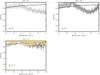 |
Fig. A.1 Observed visibility (dashed lines) dispersed over wavelengths of Y Pav observations, compared to models (full line) without mass loss. The different projected baselines are indicated in the color legend. |
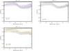 |
Fig. A.2 Observed visibility (dashed lines) dispersed over wavelengths of X TrA observations, compared to models (full line) without mass loss. The different projected baselines are indicated in the color legend. |
Appendix B: Intensity profiles and visibilities versus baselines and observing log
Photometric data from the literature.
Journal of the MIDI observations of R Vol.
Journal of the MIDI observations of U Hya.
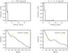 |
Fig. B.1 Interferometric observational MIDI data of U Hya compared with the synthetic visibilities based on the DARWIN models; top: intensity profile at two different wavelengths: 8.5 μm and 11.4 μm and bottom: visibility vs. baseline; the black line shows the dynamic model, the colored symbols illustrate the MIDI measurements at different baselines configurations. |
 |
Fig. B.4 uv-coverage of the MIDI observations of R Vol (left side) and U Hya (right side) listed in Tables B.2 and B.3, dispersed in wavelengths. |
All Tables
Summary of the best fitting model for each type of observation: photometry, spectroscopy, and interferometry.
All Figures
|
Fig. 1 Photometric observations of Mira stars: R Lep (left) and R Vol (right). Observations (violet circles) are compared to the DARWIN model’s synthetic photometry (gray diamonds). Orange diamonds show the best fitting time-steps of the two stars. |
| In the text | |
|
Fig. 2 Photometric observations of SRb and Lb stars: Y Pav (upper left) and AQ Sgr (upper right), and U Hya (lower left) and X TrA (lower right). Observations (violet circles) are compared to the DARWIN model’s synthetic photometry (gray diamonds). Orange diamonds show the best fitting time-steps of the four stars. |
| In the text | |
|
Fig. 3 Visibility dispersed over wavelengths of the Mira variables of our sample. Models are plotted in full lines, observations in dashed lines, at the different projected baselines (see color legend). The stars are identified in the title. The six panels show R Lep dispersed visibilities at the baseline configuration D0-A1 a); D0-B2 b); H0-I1 c); and A1-G1 d), as also marked in the plot titles. R Vol dispersed visibilities are at the baseline configuration A1-G1 e) and A1-K0 f). Error bars are of the order of 10%, and a typical error-size bar is shown in gray in each panel, overlapping with the data at 8.5 μm. In panel a), the two models’ full lines are overlapping, as the two observations lines. In panel d), the two lines of the observations are overlapping, and the model at Bp = 79 also lies on top of them. |
| In the text | |
|
Fig. 4 As in Fig. 3, for the semi-regular and irregular stars of our sample: Y Pav in panels a), b), c); X TrA in panels d), e), f); U Hya in panel g) and AQ Sgr in panel f). Error bars are of the order of 10%, and a typical error-size bar is shown in gray in each panel, overlapping with the data at 8.5 μm. Panels c), d), and f) show the two full lines (models) that overlap. |
| In the text | |
|
Fig. 5 Observational spectro-photometric data of R Lep, compared with the synthetic spectrum of the best-fitting time-step (violet). Photometry is plotted in green circles, while IRAS (Olnon et al. 1986) and NASA/IRTF (Rayner et al. 2009) spectra are plotted as black lines to allow qualitative verification of the photometric fit. The spectrum of the DARWIN models, for which the synthetic photometry fits best the corresponding observational data, is shown in violet. |
| In the text | |
|
Fig. 6 Interferometric observational MIDI data of R Lep, compared with the synthetic visibilities based on the DARWIN models; top: intensity profile at two different wavelengths: 8.5 μm and 11.4 μm and bottom: visibility versus baseline; the black line shows the dynamic model and the colored symbols illustrate the MIDI measurements at different baselines configurations. |
| In the text | |
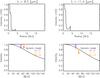 |
Fig. 7 As in Fig. 6, but for Y Pav. |
| In the text | |
|
Fig. 8 Visibilities dispersed in wavelengths for the shorter baseline (Bp = 34 m) of R Lep observations, in black. The gray lines illustrate the range in visibility of the model’s time-steps. |
| In the text | |
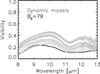 |
Fig. 9 Same as Fig. 8, but for the longest baseline of R Lep observations (Bp = 79 m). |
| In the text | |
|
Fig. 10 Visibilities vs. baselines of R Lep model, illustrating the range of available synthetic time-steps (in gray) at two chosen wavelengths: 8.5 μm and 11.4 μm. The colored squares are the R Lep observations. |
| In the text | |
|
Fig. 11 Interferometric observational MIDI data of Y Pav, in cases where the amount of SiC increased to 50% in the models, compared with the synthetic visibilities based on the DARWIN models; top: intensity profile at 11.3 μm and bottom: visibility vs. baseline. The black line shows the dynamic model, the colored symbols illustrate the MIDI measurements at different baseline configurations. |
| In the text | |
|
Fig. 12 Y Pav wavelength dependent visibilities in the MIDI range, for the only baseline configuration D0-H0, in cases where the amount of SiC increased to 50% in the models. |
| In the text | |
|
Fig. 13 AGB region of the H-R diagram. The lines display solar metallicity evolutionary tracks from Marigo et al. (2013): gray lines mark the regions of Oxygen-rich stars with C/O < 1.0; yellow lines denote the region of C-rich stars with |
| In the text | |
|
Fig. A.1 Observed visibility (dashed lines) dispersed over wavelengths of Y Pav observations, compared to models (full line) without mass loss. The different projected baselines are indicated in the color legend. |
| In the text | |
|
Fig. A.2 Observed visibility (dashed lines) dispersed over wavelengths of X TrA observations, compared to models (full line) without mass loss. The different projected baselines are indicated in the color legend. |
| In the text | |
|
Fig. B.1 Interferometric observational MIDI data of U Hya compared with the synthetic visibilities based on the DARWIN models; top: intensity profile at two different wavelengths: 8.5 μm and 11.4 μm and bottom: visibility vs. baseline; the black line shows the dynamic model, the colored symbols illustrate the MIDI measurements at different baselines configurations. |
| In the text | |
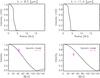 |
Fig. B.2 Same as Fig. B.1, but for AQ Sgr. |
| In the text | |
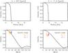 |
Fig. B.3 Same as Fig. B.1, but for X TrA. |
| In the text | |
|
Fig. B.4 uv-coverage of the MIDI observations of R Vol (left side) and U Hya (right side) listed in Tables B.2 and B.3, dispersed in wavelengths. |
| In the text | |
Current usage metrics show cumulative count of Article Views (full-text article views including HTML views, PDF and ePub downloads, according to the available data) and Abstracts Views on Vision4Press platform.
Data correspond to usage on the plateform after 2015. The current usage metrics is available 48-96 hours after online publication and is updated daily on week days.
Initial download of the metrics may take a while.