| Issue |
A&A
Volume 599, March 2017
|
|
|---|---|---|
| Article Number | A71 | |
| Number of page(s) | 13 | |
| Section | Extragalactic astronomy | |
| DOI | https://doi.org/10.1051/0004-6361/201629044 | |
| Published online | 02 March 2017 | |
Aperture-free star formation rate of SDSS star-forming galaxies⋆
1 Instituto de Astrofísica de Andalucía – CSIC, Glorieta de la Astronomía s.n., 18008 Granada, Spain
e-mail: This email address is being protected from spambots. You need JavaScript enabled to view it.
2 Estación Experimental de Zonas Áridas – CSIC, Ctra. de Sacramento s.n., La Cañada, 04120 Almería, Spain
3 Instituto Nacional de Astrofísica, Óptica y Electrónica, Luis E. Erro 1, 72840 Tonantzintla, Puebla, Mexico
Received: 2 June 2016
Accepted: 15 November 2016
Abstract
Large area surveys with a high number of galaxies observed have undoubtedly marked a milestone in the understanding of several properties of galaxies, such as star-formation history, morphology, and metallicity. However, in many cases, these surveys provide fluxes from fixed small apertures (e.g. fibre), which cover a scant fraction of the galaxy, compelling us to use aperture corrections to study the global properties of galaxies. In this work, we derive the current total star formation rate (SFR) of Sloan Digital Sky Survey (SDSS) star-forming galaxies, using an empirically based aperture correction of the measured Hα flux for the first time, thus minimising the uncertainties associated with reduced apertures. All the Hα fluxes have been extinction-corrected using the Hα/ Hβ ratio free from aperture effects. The total SFR for ~210 000 SDSS star-forming galaxies has been derived applying pure empirical Hα and Hα/ Hβ aperture corrections based on the Calar Alto Legacy Integral Field Area (CALIFA) survey. We find that, on average, the aperture-corrected SFR is ~0.65 dex higher than the SDSS fibre-based SFR. The relation between the SFR and stellar mass for SDSS star-forming galaxies (SFR-M⋆) has been obtained, together with its dependence on extinction and Hα equivalent width. We compare our results with those obtained in previous works and examine the behaviour of the derived SFR in six redshift bins, over the redshift range 0.005 ≤ z ≤ 0.22. The SFR-M⋆ sequence derived here is in agreement with selected observational studies based on integral field spectroscopy of individual galaxies as well as with the predictions of recent theoretical models of disc galaxies.
Key words: galaxies: general / galaxies: star formation / galaxies: formation / galaxies: evolution
A table of the aperture-corrected fluxes and SFR for ~210 000 SDSS star-forming galaxies and related relevant data is only available at the CDS via anonymous ftp to cdsarc.u-strasbg.fr (130.79.128.5) or via http://cdsarc.u-strasbg.fr/viz-bin/qcat?J/A+A/599/A71
© ESO, 2017
1. Introduction
In the last two decades we have witnessed the revolutionary appearance of large area surveys with a huge number of galaxies observed (e.g. Sloan Digital Sky Survey (SDSS), York et al. 2000; 2dFGRS, Colless et al. 2001; VVDS, Le Fèvre et al. 2005; GAMA, Driver et al. 2011). These surveys have been very useful for performing a complete study of the non-uniform distribution of galaxies in the Universe (large-scale structure) and to understand galaxy formation and evolution. They also give us information about important properties of galaxies, such as morphology, stellar mass, star formation rate, metallicity, and dependence on the environment. These surveys used single-fibre spectroscopy with small apertures (e.g. 2′′ diameter for 2dFGRS and GAMA, and 3′′ diameter for SDSS) and therefore cover a limited region of the galaxy, thus providing partial information on the extensive properties of galaxies. For a more detailed analysis of the integrated properties of each galaxy, it is necessary to make use of integral field spectrographs (IFS, e.g. Kehrig et al. 2012, 2016). IFS surveys, such as SAURON (Bacon et al. 2001), PINGS (Rosales-Ortega et al. 2010), MASSIV (Contini et al. 2012), CALIFA (Sánchez et al. 2012; García-Benito et al. 2015), and MANGA (Bundy et al. 2015), are based on arrays of fibres and allow us to obtain information from the whole galaxy. However, the integration times necessary to observe each galaxy are long, hindering the acquisition of a large number of galaxies in comparison with that obtained from single-fibre surveys.
It is clear that to gain a better insight into the global properties of galaxies we need tools that allow us to link both single-fibre and IFS surveys. In this work we make use of one of these tools for the purpose of studying the total current star formation rate (hereafter SFR) of star-forming galaxies, using their total Hα fluxes emitted by the gas ionised by young massive stars (e.g. Kennicutt 1998; Kennicutt et al. 2009). The SFR presents a well-known characteristic relation with the stellar mass (e.g. Brinchmann et al. 2004b). In the SFR-stellar mass plane (SFR-M⋆), active star-forming galaxies define a distinct sequence called main sequence (Noeske et al. 2007). In addition, less active star-forming galaxies (e.g. quenched and ageing star-forming galaxies) appear in this plane located at higher masses and lower SFR values (e.g. Renzini & Peng 2015; Casado et al. 2015; Leslie et al. 2016), as well as a family of outliers to this main sequence (MS) that are generally interpreted as starbursts driven by merging (e.g. Rodighiero et al. 2011). The MS of star formation has been parametrized by the following equation:  (1)From a theoretical point of view, recent studies have obtained values for α (MS slope) near to unity (e.g. Dutton et al. 2010; Sparre et al. 2015; Tissera et al. 2016). Dutton et al. (2010) used a semi-analytic model of disc galaxies parametrizing several properties: for example, SFRs and metallicities were computed in a spatially resolved way as a function of galactic radius. For galaxies with stellar masses between 109M⊙ and 1011M⊙ the slope found in Dutton et al. (2010) is α = 0.96. In contrast, Sparre et al. (2015) used Illustris (state-of-the-art cosmological hydrodynamical simulation of galaxy formation; Nelson et al. 2015) to reproduce the observed star formation MS, finding a similar slope to Dutton et al. (2010) at low redshift. From observational studies quoting Hα based SFR determinations, the MS slope varies preferentially between ~0.6 and ~1, and β between ~–9 and ~–3, depending on the precise methodology and data used (see e.g. Rodighiero et al. 2011; Speagle et al. 2014, and references therein). An important factor behind this spread in α and β values can be related to the aperture corrections applied to the Hα measurements.
In order to evaluate the SFR of a galaxy in single-fibre surveys, an aperture correction needs to be applied to account for the entire galaxy. This correction becomes essential in order to analyse the SFR dependence with redshift (z), especially for samples of star-forming galaxies at low z. Many such studies have dealt with the SFR of star-forming galaxies in the local Universe (e.g. Brinchmann et al. 2004b; Iglesias-Páramo et al. 2006; Salim et al. 2007; Kennicutt et al. 2008; Peng et al. 2010) and others extended to medium and large redshift (e.g. Madau et al. 1996; Elbaz et al. 2007; Peng et al. 2010; Whitaker et al. 2012; Drake et al. 2013, 2015). At lower redshift the effects produced by a fixed aperture size will be clearly more significant than for high redshifts. It is important to note that for galaxies about the size of the Milky Way, the 3-arcsec-diameter SDSS fibre never encompasses the complete galactic disc. For this reason, it is always necessary to use aperture corrections to derive the total SFR when using the SDSS Hα fluxes. An extra drawback produced by this limitation of the SDSS fibre is particularly relevant for “late-type” spiral galaxies (i.e. disc-dominated galaxies with Hubble type from Sb to Sdm, Dahlem 1997) since they present higher star formation in the outer parts of their discs. Therefore, the Hα flux measured by SDSS for these galaxies would lead to an underestimation of the total SFR.
Several studies have already emphasised the importance of quantifying the effect of aperture in the observational data (e.g. Kewley et al. 2005; Kennicutt et al. 2008; Mast et al. 2014) and also when comparing with the theoretical model predictions (Guidi et al. 2016). To our knowledge, a solid empirical aperture correction has not yet been implemented in a systematic way for the analysis of large samples of galaxies. Up to now, most studies quantifying the total SFR of galaxies from single-fibre surveys apply aperture corrections using model-based methods (e.g. Brinchmann et al. 2004b; Salim et al. 2007). Other works apply geometrical considerations in order to compensate for the unobserved Hα emission of the galaxy, scaling it according to its broad-band photometric map, or by using analytical recipes (e.g. Hopkins et al. 2003, 2013). For SDSS star-forming galaxies, Brinchmann et al. (2004b) originally corrected SDSS fibre SFRs from aperture effects using the resolved colour information available for each galaxy. In the Max-Planck-Institut für Astrophysik and Johns Hopkins University (MPA-JHU) database1 (Kauffmann et al. 2003b; Brinchmann et al. 2004b; Tremonti et al. 2004; Salim et al. 2007) the Brinchmann et al. (2004b) methodology, improved following Salim et al. (2007), was used to derive SFRs. It is important to note that MPA-JHU galactic SFRs always include the nuclear emission. In addition, the median profiles of the growth curve corresponding to the Hα/ Hβ aperture correction decreases when galaxy radius increases (Iglesias-Páramo et al. 2013). Thus, galaxies for which only the central zones are observed present overestimated extinction (Iglesias-Páramo et al. 2016, hereafter IP16): on average, some bias is expected in MPA-JHU SFRs since galaxies’ extinction gradients were not accounted for (Richards et al. 2016).
A rigorous methodology to derive the total SFR of a galaxy should make use of its entire Hα flux and Hα/ Hβ ratio. For single-fibre surveys, the total Hα flux of a galaxy can be obtained using an empirical aperture correction for Hα derived from IFS of nearby galaxies. According to Iglesias-Páramo et al. (2013, 2016), the CALIFA project allows an accurate aperture correction for Hα to be derived empirically. IP16 provide the growth curve of Hα flux as a function of R50, the Petrosian radius containing 50% of the total galaxy flux in the r-band, on the basis of a representative sample of 165 star-forming galaxies from the CALIFA survey (Sánchez et al. 2012; Husemann et al. 2013; Walcher et al. 2014). In this work we make use of the empirical aperture correction from IP16 in order to obtain the total Hα flux for a sample of ~210 000 star-forming galaxies from the SDSS. From this total Hα flux we derive aperture-corrected values of SFR in each galaxy, which will allow us to study the global relation between the SFR, stellar mass, and redshift.
To our knowledge this work represents the first attempt to analyse the behaviour of the present-day SFR for a large sample including all SDSS star-forming galaxies using the total Hα emission empirically corrected by Hα aperture coverage in a systematic manner. The structure of this paper is organised as follows. In Sect. 2 we describe the data and provide a description of the methodology used to select the star-forming galaxies. We detail the methodology used to derive the entire Hα flux using the empirical aperture correction and the corresponding SFR in Sect. 3. Our main results are presented in Sect. 4 and the associated discussion in Sect. 5. Finally, a summary and the main conclusions of our work are given in Sect. 6.
Throughout the paper, we assume a Friedman-Robertson-Walker cosmology with ΩΛ0 = 0.7, Ωm0 = 0.3, and H0 = 70 km s-1 Mpc-1. We use the Kroupa (2001) universal initial mass function (IMF)2.
2. Data and sample
2.1. Sample selection
Our study is based on the MPA-JHU public catalogue (Kauffmann et al. 2003b; Brinchmann et al. 2004b; Tremonti et al. 2004; Salim et al. 2007), which gives spectroscopic data of the galaxies in the Sloan Digital Sky Survey Data Release 7 (SDSS-DR7) (Abazajian et al. 2009). The SDSS spectroscopic primary sample of galaxies is complete in Petrosian r magnitude in the range 14.5 ≤ r ≤ 17.7 (Strauss et al. 2002; Brinchmann et al. 2004a). We added the photometric data from the SDSS-DR12 (York et al. 2000; Alam et al. 2015) to the MPA-JHU catalogue. The MPA-JHU catalogue contains 1 477 411 objects, of which 933 310 are galaxies with spectroscopic properties. In this catalogue, the stellar masses are estimated using spectral energy distribution (SED) fitting to ugriz photometry as described in Kauffmann et al. (2003b). The line fluxes3 are corrected for foreground Galactic reddening and extinction using the attenuation curve from O’Donnell (1994) and the extinction from Schlegel et al. (1998). Finally, MPA-JHU provides the emission line fluxes measured using Gaussian fittings over the subtracted continuum and the signal-to-noise (S/N) in the whole spectrum. For those galaxies with multiple entries we selected only those with the largest S/N in the whole spectrum, reducing the total number of galaxies to 874 701.
We selected our primary sample according to the following criteria:
-
i)
The galaxy stellar mass [log (M⋆/M⊙)] is selected in the range between 8.50 and 11.50. Galaxies without any estimation of the stellar mass are discarded in order to carry out a proper comparison between the SFR and the stellar mass.
-
ii)
We restricted our sample to the galaxies with small relative error of size measurements of R50 (Δ(R50) /R50 ≤ 1/3). In agreement with this consideration, we removed those galaxies with Δ(R50) /R50 greater than 1/3, which may be detrimental for our study when we use the growth curves from IP16 in order to derive the aperture corrected Hα flux (as will be explained in Sect. 3.1).
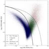
Fig. 1 [OIII] λ 5007/Hβ versus [NII] λ 6583/Hα diagnostic diagram (BPT) for the SDSS galaxies. Blue, green, and red points represent star-forming galaxies in the present work (209 276), composite galaxies (57 926), and AGN galaxies (19 392), respectively. The dashed line shows the Kewley et al. (2001) demarcation and the continuous line shows the Kauffmann et al. (2003a) curve.
-
iii)
We considered galaxies with values for 1.5′′/R50 higher than 0.3 (i.e. R50 ≤ 5′′), where 1.5′′ is the radius of the SDSS fibre. Iglesias-Páramo et al. (2013) showed that the seeing may affect the Sérsic profile for values below this cut-off limit for the parameter 1.5′′/R50, according to the analytical study carried out by Trujillo et al. (2001). The full width at half maximum (FWHM) of the point spread function (PSF) has a median value of ~3.6′′ in the CALIFA observations (Husemann et al. 2013; Iglesias-Páramo et al. 2013).
-
iv)
We did not consider galaxies whose SDSS spectra were classified as quasi stellar objects (QSO). In the original catalogue we have found 14 476 QSO galaxies.
-
v)
Spectroscopic redshift in the range 0.005 ≤ z ≤ 0.22. The lower z-limit of 0.005 was adopted in order to: a) minimise the effect in the photometric measurements for the larger nearby galaxies; b) to include galaxies with the lowest luminosities (Brinchmann et al. 2004b). It is expected that a sizeable fraction of the low luminosity SDSS galaxies could remain unobserved for the redshift range considered (e.g. Blanton et al. 2005).
2.2. Selection of the star-forming galaxies
We selected a subset of 209 276 star-forming galaxies from our primary sample described in Sect. 2.1 (31.92% from our primary sample in Sect. 2.1) applying the following criteria:
-
i)
The S/N is greater than three for the fluxes in the strong emission lines Hα, Hβ, [OIII] , and [NII]. We have defined the S/N as the ratio of the flux and the statistical error flux, calculated with the pipeline described in Tremonti et al. (2004) (Kewley & Ellison 2008). Below this limit in S/N, an important fraction of galaxies present negative line fluxes (Brinchmann et al. 2004b).
-
ii)
We selected the pure star-forming galaxies according to the Kauffmann definition in the BPT diagnostic diagram (e.g. Baldwin et al. 1981; Veilleux & Osterbrock 1987; Kewley et al. 2001; Kauffmann et al. 2003a): [OIII] λ 5007/Hβ versus [NII] λ 6583/Hα (see Fig. 1):
![Mathematical equation: \begin{equation} \label{Eq:eq_2} \rm log([OIII]/H\beta) \leq {{0.61}\over{[log([NII]/{\rm H\alpha})-0.05]}}+1.3. \end{equation}](/articles/aa/full_html/2017/03/aa29044-16/aa29044-16-eq31.png) (2)log ([OIII] /Hβ) values below this curve imply
a contribution to Hα from active galactic nuclei (AGN) less than
1%, (i.e. discarding
composite or AGN galaxies; Kauffmann et al.
2003a; Brinchmann et al. 2004b)4.
(2)log ([OIII] /Hβ) values below this curve imply
a contribution to Hα from active galactic nuclei (AGN) less than
1%, (i.e. discarding
composite or AGN galaxies; Kauffmann et al.
2003a; Brinchmann et al. 2004b)4. -
iii)
The Hα equivalent width (EW(Hα))5 is greater than or equal to three. This condition is assumed to avoid passive galaxies as defined by Cid Fernandes et al. (2011).
In Table 1 we present the median (±1σ confidence interval)6 of several parameters split into six redshift bins within the range 0.005 ≤ z ≤ 0.22. In Col. 1 the Δz is presented, Col. 2 shows the log (M⋆/M⊙), Cols. 3 and 4 show the S/N for the Hα emission line flux and the S/N per whole spectrum range, respectively; the EW(Hα) is presented in Col. 5, Col. 6 displays the R50, and the number of galaxies per redshift bin is quoted in Col. 7.
Values of relevant parameters corresponding to the median (±1σ confidence interval) of the distribution for the star-forming galaxies in six redshift bins up to z = 0.22 in the total sample.
3. Empirical aperture correction and derivation of the SFR
3.1. Empirical aperture correction
The fact that SDSS fibres (3′′ diameter) cover only a limited region of a galaxy at low-redshift Universe (z< 0.22), implies that only a limited amount of Hα emission can be measured. In order to derive the total Hα flux of each galaxy in our final sample, we corrected the SDSS Hα fluxes for aperture using the empirical aperture corrections in IP167. IP16 provide aperture corrections for emission lines and line ratios in a sample of spiral galaxies from the CALIFA database. Median growth curves of Hα and Hα/ Hβ, up to 2.5 R50, were computed to simulate the effect of observing galaxies through apertures of varying radii. The median growth curve of the Hα flux (the Hα/ Hβ ratio) shows a monotonous increase (decrease) with radius, with no strong dependence on galaxy properties (i.e. inclination, morphological type, and stellar mass). The IP16 sample of CALIFA star-forming galaxies spans over the whole range in galaxy mass studied in this work (see IP16 for more details).
To strengthen the relevance of the CALIFA star-forming galaxies sample used in this work for the analysis of SDSS star-forming galaxies, a series of tests have been performed. First, the similarity between the galaxy stellar mass distributions of both samples has been statistically confirmed applying a Kolmogorov-Smirnov (KS) test, from which the following results have been obtained: Dn1,n2 = 0.08 and p-value = 0.36, indicating that we cannot reject the hypothesis that both samples are drawn from the same distribution. Second, the relations between SFR-M⋆ and galaxy size-M⋆ for star-forming galaxies from CALIFA and SDSS samples have been analysed (see Appendix A); conclusive positive results have been achieved showing how the medians of the SFR of CALIFA galaxies are consistent with the results obtained in this work for SDSS galaxies over the whole range of galaxy mass (see Fig. A.1). Likewise for the galaxy size-M⋆ relation, the plot of R50 vs. M⋆ (see Fig. A.2) shows that the medians of CALIFA galaxies are clearly consistent with the SDSS galaxies distribution.
SDSS Hα fluxes were previously corrected for extinction using the Balmer decrement as measured by the Hα/ Hβ ratio (FHα/ Hβap, corr). To do so, the median Hα/ Hβ flux ratio growth curve normalised to the Hα/ Hβ flux ratio at 2.5 R50, X(αβ50), was applied to each galaxy, and the Hα/ Hβ ratio was computed according to its corresponding value of 1.5 /R50 following IP16:  (3)being
 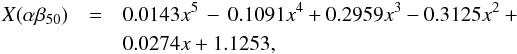 where x = (1.5 /R50) for each galaxy, FHα/ Hβ0 is the SDSS Hα/ Hβ ratio.
Theoretical case B recombination was assumed (the theoretical Balmer decrement, IHα/ Hβ = 2.86; T = 104K, and low-density limit ne ~ 102 cm-3; Osterbrock 1989; Storey & Hummer 1995) together with the Cardelli et al. (1989) extinction curve with Rv = Av/E(B−V) = 3.1 (O’Donnell 1994; Schlegel et al. 1998).
Equation (4) presents the aperture-corrected Hα flux,  , as a function of the Hα flux in the SDSS fibre,
  , and the X(α50), the median Hα flux growth curve normalised to the Hα flux at 2.5 R50:
  (4)being
X(α50) = 0.0037x5 + 0.0167x4−0.2276x3 + 0.5027x2 + 0.1599x where x = (1.5 /R50) for each galaxy. According to IP16, for an aperture radius of 2.5 R50 an average of ~85% of the total Hα flux of (non-AGN) spiral galaxies is enclosed.
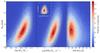 |
Fig. 2 Density plots for the SDSS star-forming galaxies: i) left panel: the relation between log (M⋆/M⊙) and A(Hα); ii) central panel: the relation between log (SFR/M⊙ yr-1) and A(Hα), the inset plot shows the A(Hα)-log (sSFR/Gyr-1) relation; iii) right panel: the relation between EW(Hα) and A(Hα). The dashed lines represent the 1σ, 2σ, and 3σ contours. |
Equation (5) presents the total Hα flux,  , corrected for aperture effects and extinction:
 ![Mathematical equation: \begin{equation} \label{Eq:eq_5} F_{{\rm H\alpha}}^{\rm tot}=\dfrac{F_{{\rm H\alpha}}^{\rm ap,\ corr}}{10^{-0.4\,A({\rm H\alpha})}},\\[1ex] \end{equation}](/articles/aa/full_html/2017/03/aa29044-16/aa29044-16-eq113.png) (5)where the extinction in Hα, A(Hα) = 1.758 c(Hβ). The reddening coefficient is
(5)where the extinction in Hα, A(Hα) = 1.758 c(Hβ). The reddening coefficient is  , and f(Hα) is the reddening curve.
3.2. Aperture-corrected star formation rate
The present day SFR is defined as the stellar mass formed per unit time traced by the young stars. The SFR can be derived from the Hα luminosity, and it is parametrized as SFR = L(Hα) /ηHα, the ratio of observed Hα luminosity8 to the conversion factor ηHα (Brinchmann et al. 2004b). The parameter ηHα varies with the physical properties of the galaxy, total stellar mass, and metallicity (see Charlot et al. 2002; Hirashita et al. 2003; Brinchmann et al. 2004b).
Kennicutt et al. (2009) assumed ηHα is a constant value, ηHα = 1041.26 erg/s /M⊙/ yr, which resulted in a good typical conversion factor, though ηHα can in fact vary as much as ~0.4 dex going from the least to the most massive galaxies (Brinchmann et al. 2004b). In order to parametrize the variation of the ηHα as a function of stellar mass, we have used the median of the ηHα likelihood distribution for the five stellar mass ranges as shown in Fig. 7 in Brinchmann et al. (2004b): log (M⋆/M⊙) < 8; 8 < log (M⋆/M⊙) < 9; 9 < log (M⋆/M⊙) < 10; 10 < log (M⋆/M⊙) < 11; log (M⋆/M⊙) > 11. The relation between ηHα and galaxy stellar mass has been parametrized through a two-order polynomial fit as presented in Eq. (6):  (6)where x = log (M⋆/M⊙). We used the values of ηHα from Eq. (6) to calculate the SFR = L(Hα) /ηHα for our galaxy sample. Hereafter, we refer to the aperture-corrected log (SFR)−log (M⋆) relation as the SFR-M⋆ relation for our sample of galaxies. Also, from now on we refer to the SFR and the specific SFR (sSFR = SFR/M⋆) derived here as the empirical aperture-corrected SFR and sSFR for star-forming galaxies.
Notwithstanding the above, possible effects associated with, for example, diffuse ionised gaseous emission, geometry, or galaxy inclination should be considered (e.g. Relaño et al. 2006; Kennicutt et al. 2009; Kennicutt & Evans 2012; van der Wel et al. 2014). Although a comprehensive study of these effects could be hard to handle (e.g. Kennicutt & Evans 2012), recent work by Iglesias-Páramo et al. (2013, 2016) concluded that the Hα flux growth curve and the Hα/ Hβ are insensitive to the galaxy inclination for a broad range of b/a (i.e. galaxy diameters ratio) including from edge-on to face-on galaxies. The effects of the geometry of the HII regions and the contribution of the diffuse ionised gas component are more difficult to quantify. We believe that these effects should be statistically minimised in this work, given the size of the sample and the large diversity of galaxy types used in IP16.
4. Results
4.1. Extinction of the star-forming galaxies in the SDSS sample
The extinction suffered by the Hα photons, A(Hα), derived in this work goes from 0 to 2 mag, with a median of A(Hα) = 0.85 mag9 (in agreement with previous work: Buat et al. 2002; Hopkins et al. 2003; Brinchmann et al. 2004b; Nakamura et al. 2004; Momcheva et al. 2013). A(Hα) presents a strong dependence with galaxy mass, as shown in Fig. 2 (left panel), being larger for more massive galaxies, (see Brinchmann et al. 2004b; Whitaker et al. 2012; Momcheva et al. 2013; Koyama et al. 2015). Moreover, A(Hα) shows a trend with the SFR, with A(Hα) ≤ 0.2 mag for those galaxies presenting the lowest SFR (log (SFR/M⊙ yr-1) ≈ −0.5) whereas the highest values of A(Hα) are associated with the galaxies with the largest SFR (Fig. 2 central panel). Only a mild trend can be appreciated when A(Hα) is plotted versus the sSFR, confirming the strong weight that galaxy stellar mass has in the variation of A(Hα). The behaviour of A(Hα) as a function of EW(Hα) is shown in Fig. 2 (right panel). Galaxies showing the median value of A(Hα) cluster around EW(Hα) ~ 15 Å. For EW(Hα) > 30 Å, A(Hα) presents a strong decline, approximating to values near 0.2 mag and lower for EW(Hα) above 60 Å. An upper envelope for the maximum of the A(Hα) can be seen, decreasing towards larger values of EW(Hα).
The results presented above tell us that the A(Hα) extinction correction can be substantial and therefore must be applied to all galaxy samples to be used in the study of the SFR. Moreover, these results also show that the behaviour of A(Hα) appears to be different depending on the EW(Hα) of star-forming galaxies, showing a strong relation with galaxy mass and total SFR (see e.g. Koyama et al. 2015).
4.2. Parametrizing the aperture-corrected SFR-M⋆ relation for star-forming galaxies
In Fig. 3 we present the aperture-corrected SFR-M⋆ relation for our sample of star-forming galaxies (see Sect. 2.2). The SDSS fibre flux for each galaxy was corrected for aperture and extinction as explained in Sect. 3.1. The SFR was derived for each galaxy of the sample applying the methodology described in Sect. 3.2. The running median of the distribution of points plotted in Fig. 3 (red solid line) has been fitted with the following analytical expression:  (7)where x = log (M⋆/M⊙).
For the sake of comparison with previous work (see Sect. 5), a straight linear fit to the running median distribution in Fig. 3 has been obtained as follows:  (8)where slope α = 0.935( ± 0.001), β = −9.208( ± 0.001), and x = log (M⋆/M⊙).
Figure 3 also shows the three-order polynomial fit to the running median of the values of SFR computed from the SDSS fibre flux without any correction by aperture (green dashed line). It is clear from Fig. 3 that the corrected SFR is, on average, more than 0.65 dex above the values corresponding to the SDSS fibre flux. The SFR-M⋆ relation obtained is consistent with the relation shown by Catalán-Torrecilla et al. (2015) for their sample of star-forming galaxies of the CALIFA survey (see Fig. A.1).
The inset plot shows the sSFR-M⋆ relation for our sample, corrected for aperture and extinction. The fits to the running medians of the aperture-corrected sSFR-M⋆ (red solid line) and the SDSS fibre fluxes (green dashed line) are also shown. From the sSFR-M⋆ relation, we observe that the fit to the running median distribution is decreasing slightly for the entire stellar mass range selected, consistent with recent predictions (see e.g. Sparre et al. 2015, and references therein).
For the sake of completeness, in Table 2 we present median values (±1σ confidence interval) of the derived log (SFR) for twelve stellar mass bins (Δlog (M⋆/M⊙) = 0.25 dex each) within the range 8.5 ≤ log (M⋆/M⊙) ≤ 11.5. In Col. 1 the range of log (M⋆/M⊙) is presented, Col. 2 shows the log (SFR/M⊙ yr-1), and the number of galaxies per stellar mass bin is quoted in Col. 3.
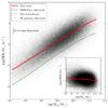 |
Fig. 3 Relation between the SFR and M⋆ for star-forming galaxies. The red solid line and green dashed line represent the fit to the running median for bins of 2000 objects in this work and in the SDSS fibre, respectively. The red dotted line represents the linear fit to the running median for bins of 2000 objects in this work. The vertical black line shows the 1σ average dispersion (~0.3 dex). The inset plot shows the sSFR-M⋆ relation for our sample and the running median, for bins of 2000 objects, for the sSFR corrected for aperture (red solid line) and inside the SDSS fibre (green dashed line). |
Values of aperture-corrected SFR corresponding to the median (±1σ confidence interval) of the distribution for the star-forming galaxies in twelve stellar mass bins in the total sample.
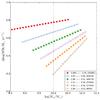 |
Fig. 4 Empirical SFR corrections (total – SDSS fibre) vs. M⋆ relation. Red, blue, green, magenta, orange, and gold lines represent the fit to the running median for bins of 1000 objects in six redshift bins up to z = 0.22 for a sample of star-forming galaxies. The numbers of star-forming galaxies in each redshift bin appear on the legend. The vertical black dotted line corresponds to the reference value at log (M⋆/M⊙) = 10. |
4.3. Aperture-corrected SFR as a function of the M⋆ and z interval
The aperture-corrected SFR as a function of the M⋆ is studied in six redshift bins in the range 0.005 ≤ z ≤ 0.22. Figure 4 presents this evolution for the star-forming galaxy sample in the following redshift intervals: 0.005 ≤ z < 0.05, 0.05 ≤ z < 0.08, 0.08 ≤ z < 0.11, 0.11 ≤ z < 0.14, 0.14 ≤ z < 0.18, and 0.18 ≤ z ≤ 0.22. In this figure, for each z range, the corresponding line is the fit to the running median of the differences between the aperture-corrected SFR and the SFR within the SDSS fibre as a function of the M⋆.
This figure shows that: i) over the whole range of galaxy stellar masses studied, the average aperture correction goes from ~0.7 to ~0.8 for 0.005 ≤ z ≤ 0.05; ii) aperture corrections increase with galaxy mass for each redshift interval for 0.05 ≤ z ≤ 0.22; reaching from ~0.2 for log (M⋆/M⊙) = 10 to ~0.6 for log (M⋆/M⊙) = 11, for 0.18 ≤ z ≤ 0.22.
In Table 3, for each z range, we present the median (±1σ confidence interval) of the derived log (SFR/M⊙ yr-1) and log (M⋆/M⊙) along three stellar mass bins and for the whole mass range (8.5 ≤ log (M⋆/M⊙) ≤ 11.5) for six redshift bins in the range 0.005 ≤ z ≤ 0.22. In Col. 1 the Δz is displayed, the Δlog (M⋆/M⊙) is presented in Col. 2, Col. 3 shows the log (SFR/M⊙ yr-1), Col. 4 shows the log (M⋆/M⊙), and the number of galaxies per stellar mass bin is quoted in Col. 5. All this information is presented in Fig. 5 for the sample of galaxies in the range of redshift and stellar mass considered. In this figure we show the relation between total SFR and M⋆ for our sample of star-forming galaxies, along three stellar mass bins for the whole mass range (8.5 ≤ log (M⋆/M⊙) ≤ 11.5), and for six redshift bins in the range 0.005 ≤ z ≤ 0.22.
Values of stellar mass and aperture-corrected SFR per stellar mass and redshift bins corresponding to the median (±1σ confidence interval) of the distribution for the star-forming galaxies in the total sample.
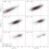 |
Fig. 5 Relation between the SFR and M⋆ for SDSS star-forming galaxies, along three stellar mass bins for the whole mass range (8.5 ≤ log (M⋆/M⊙) ≤ 11.5) and for six redshift ranges in the range 0.005 ≤ z ≤ 0.22. The black solid line represents the fit to the running median for bins of 1000 objects in this work for each redshift range. Red dots represent the medians of SFR and M⋆ per stellar mass bin and redshift range. The error bars in x- and y-axis represent the ±1σ confidence interval for stellar mass and SFR, respectively. The symbol sizes increase with the number of objects contained in each mass range. |
5. Discussion
We start by comparing our SFR values (Sect. 3.2) with the ones provided by the MPA-JHU database10. The MPA-JHU database gives the SFR within the 3′′ fibre of the SDSS and the total SFR corrected for aperture (Brinchmann et al. 2004b; Salim et al. 2007) (hereafter SFRMPA). Brinchmann et al. (2004b) originally corrected fibre SFRs from aperture effects using the resolved colour information available for each galaxy. Salim et al. (2007) noted an overestimation of these SFRs for galaxies with low levels of star formation, attributed to the larger contribution from dusty high-metallicity starbursts inside these galaxies11. Consequently, these authors improved the Brinchmann et al. (2004b) technique (see Salim et al. 2007, for a detailed description) and several studies have used these values of SFR reported by these authors (e.g. Zahid et al. 2012; Renzini & Peng 2015).
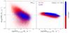 |
Fig. 6 Left panel: difference, Δlog (SFR), of total SFR provided by MPA-JHU (Brinchmann et al. 2004b; Salim et al. 2007) and our total empirical SFRThis work as a function of SFRThis work; right panel: difference of the total SFR derived using the Hopkins et al. (2003) aperture correction for the Hα flux and SFRThis work as a function SFRThis work. Upper numbers represent the number of high- (red points) and low-level (blue points) Hα emitting galaxies (colour–coded according to the EW(Hα) colour bar). The black dashed line indicates Δlog (SFR) = 0. |
A different aperture correction was applied by Hopkins et al. (2003), assuming that the Hα emission-line flux can be traced across the whole galaxy by the r-band emission. Hopkins et al. (2003) derived the total Hα flux as a function of the difference between the total petrosian r-band magnitude (rpetro) and the corresponding magnitude inside the SDSS fibre (rfibre) as:  (see also Pilyugin et al. 2013). For the sake of comparison, the total Hα flux and the corresponding L(Hα) and SFR for all the galaxies in our final sample was recalculated according to the aperture correction recipe from Hopkins et al. (2003) (Eq. (B3)). Here we have refined the Hopkins et al. (2003) recipe for Hα flux aperture correction following the methodology explained in Sect. 3.2. The only difference between our refined Hopkins et al. (2003) recipe and Hopkins et al. (2003) methodology is that the former is based on Eq. (6) which converts Hα into SFR, while the latter uses a constant conversion value of 41.26.
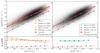 |
Fig. 7 SFRThis work−M⋆ relation for star-forming galaxies compared with previous theoretical and observational works. Comparison with observational studies: Panel a) SFR-M⋆ fits to the running median for bins of 2000 objects obtained in this work (red solid line) and from the SDSS fibre (brown dashed line), together with the values provided by MPA-JHU (blue dotted line), using the Hopkins et al. (2003) recipe (orange solid line), and from our refined method of Hopkins et al. (2003) recipe (orange dashed line). Panel b) Difference vs. M⋆ between SDSS fiber SFRs and SFRThis work and between observational studies and SFRThis work (colours as in upper left panel). Dotted line shows Δlog (SFR) = 0. Comparison with theoretical studies: Panel c) SFR-M⋆ fits to the running median for bins of 2000 objects obtained in this work (red solid line) and from the SDSS fibre (brown dashed line), together with the predictions from Sparre et al. (2015) (green dashed line) and Dutton et al. (2010; cyan dashed line). Panel d) Difference vs. M⋆ between SDSS fiber SFRs and SFRThis work and between theoretical predictions and SFRThis work (colours as in upper right panel). Dotted line shows Δlog (SFR) = 0. |
In Fig. 6 (left plot) we show the difference between SFRMPA and the empirical SFR derived in this work (SFRThis work) as a function of SFRThis work. In the right plot we present the difference between the SFR derived applying the Hopkins et al. (2003) aperture correction and SFRThis work as a function of SFRThis work. We discriminate between high- (EW(Hα) ≥ 40 Å; blue points) and low-level (EW(Hα) < 40 Å; red points) Hα emitting galaxies. The left plot shows that: i) a significant scatter is present, especially for the low-level Hα emitters, being critical (over 1 dex) for low SFRs; and ii) those galaxies with large SFRs and high EW(Hα) show values of SFRMPA somewhat closer to the ones derived in this work, though large systematic differences and big scatter remain. In the right plot, the average SFR values derived according to Hopkins et al. (2003) show a systematic difference with respect to SFRThis work ones, and a significant scatter (up to ~1 dex) is apparent. Galaxies with EW(Hα) < 40 Å present a larger scatter and a clear offset from those with EW(Hα) ≥ 40 Å. The differences between the SFR values derived using Hopkins et al. (2003) recipe and the ones obtained in this work could be reduced when we refine the Hopkins et al. (2003) methodology, as explained above; however, a noticeable scatter and some systematics between red and blue points remain. In this regard, we should bear in mind that the r-band flux of star-forming galaxies includes a contribution from Hα and nearby emission lines and, in fact, should behave as a rough tracer of HII regions. On the other hand, we note in passing that those objects with prominent bulges (likely correlating with the lower level star-formation objects in this sample) should contribute to the emission in the r-band in a more significant manner (e.g. Richards et al. 2016).
In Fig. 7 we show the SFRThis work versus M⋆ for each galaxy in our sample and compare the fit to the SFR-M⋆ relation derived with previous results from theoretical and observational works. We present (panel a) the linear fit to the running median to the SFR-M⋆ relation: i) using the empirical total SFR from this work; ii) based on the SFRMPA; iii) SFR that we obtained applying the Hopkins et al. (2003) recipe and also our refined method of Hopkins et al. (2003) recipe; iv) SFR for the Hα SDSS fibre flux derived in this work. Finally, in this figure (panel c) we also show recent theoretical predictions for the SFR vs. M⋆ relation from i) Sparre et al. (2015) at z = 0 using the Illustris simulation for star-forming galaxies with stellar masses between 109M⊙ and 1010.5M⊙; and ii) by Dutton et al. (2010) at z = 0 using a semi-analytic model for star-forming galaxies with stellar masses between 109M⊙ and 1011M⊙. In Fig. 7 (panels b and d) we present the differences between the fit to the SFR-M⋆ relation of this work and those obtained for MPA-JHU, Hopkins et al. (2003), our refined method of Hopkins et al. (2003) recipe, Dutton et al. (2010), and Sparre et al. (2015). The difference between the aperture-corrected SFR in this work and the SFR corresponding to the SDSS fibre is also shown.
As we can see in Fig. 7, the overall difference between SFRMPA and this work amounts to ~0.6 dex going from the less to the more massive galaxies. The fit to the SFR-M⋆ relation shows that SFRMPA leads to systematically larger values of the SFR for masses M⋆/M⊙< 109 (≈0.35 dex) and conversely, under-predicts the SFR12 by ≈0.3 dex for M⋆/M⊙> 1011. Recent studies have reached similar results (e.g. Richards et al. 2016)13. In this respect, we should bear in mind that galaxies with log (M⋆/M⊙) ≳ 10.5 may host large bulges containing little star formation, and therefore for these objects aperture correction can be problematic (e.g. Brinchmann et al. 2004b; Momcheva et al. 2013; Richards et al. 2016). Conversely, for less massive galaxies, the aperture problems become considerably smaller. The empirical SFR-M⋆ fit of this work also shows a systematic difference with the relation derived using Hopkins et al. (2003). The fit to the points obtained with the refined method of the Hopkins et al. (2003) recipe presented here gives a much better result. Excellent agreement is found with the Sparre et al. (2015) and Dutton et al. (2010) predictions.
It is important to note that the MS slope obtained from SFRMPA is ~0.71. As far as we know, those studies that used the SFR values from the MPA-JHU catalogue obtained similar slopes (e.g. Elbaz et al. 2007; Zahid et al. 2012; Renzini & Peng 2015, show slopes of 0.77, 0.71, 0.76, respectively). On the other hand, as mentioned in Sect. 4.2 (see Eq. (8)), the MS slope obtained in this work is 0.935. The MS slope calculated in this work is in very good agreement with the predictions of semi-analytical models by Dutton et al. (2010), giving a zero point of the MS relation consistent with our result. Agreement is also found after the comparison of the MS slope with the predictions of the Illustris cosmological hydrodynamical simulations of galaxy formation by Sparre et al. (2015).
Finally, the SFR-M⋆ relation obtained in this work appears consistent with recent IFS observations of modest-size samples of galaxies (e.g. Catalán-Torrecilla et al. 2015; Richards et al. 2016). This concordance is relevant given the fact that total SFR values by Catalán-Torrecilla et al. (2015) and Richards et al. (2016) are obtained integrating the Hα flux over the spatially resolved galaxies, whereas in this work total SFRs are derived from the SDSS fibre Hα flux corrected for aperture effects.
6. Summary and conclusions
This work provides a robust study of the total empirical SFR of galaxies and its dependence on stellar mass, extinction, and redshift. Here we present the first study that uses total Hα flux, corrected for aperture from empirical Hα growth curves, to analyse the behaviour of present-day SFR and sSFR of all SDSS star-forming galaxies. This empirical aperture correction is based on a sample of 165 spiral galaxies from the CALIFA project (IP16). Concurrently, we have derived the SFR-M⋆ and the sSFR-M⋆ relations applying our considerations. We have compared these relations, free from aperture effects, with other methods (e.g. Hopkins et al. 2003; Brinchmann et al. 2004b) and with predictions from recent theoretical models (e.g. Dutton et al. 2010; Sparre et al. 2015).
Our main conclusions are the following:
-
i)
The mean empirical aperture-corrected SFR, averaged over galaxy stellar mass, for the entire sample of SDSS star-forming galaxies amounts to ~0.65 dex.
-
ii)
The average aperture-corrected SFR for nearby galaxies, 0.005 ≤ z ≤ 0.05, is between ~0.7 and ~0.8. For larger z(0.05 ≤ z ≤ 0.22) aperture corrections increase with galaxy mass along each redshift interval.
-
iii)
The aperture-free SFR-M⋆ relation obtained in this work is: log (SFR) = 0.935( ± 0.001)log (M⋆/M⊙)−9.208( ± 0.001). When comparing total SFRs from previous works with ours, we find: a) the SFR-M⋆ relation by MPA-JHU (Brinchmann et al. 2004b; Salim et al. 2007) provides larger SFR values (by ~0.3 dex) for log (M⋆/M⊙) ≤ 9; conversely, MPA-JHU SFR values for log (M⋆/M⊙) ≥ 11 appear systematically lower (by up to 0.3 dex); b) overall consistency is found with selected observational studies based on integral field spectroscopy of individual galaxies (e.g. Catalán-Torrecilla et al. 2015; Richards et al. 2016); c) excellent agreement is obtained with theoretical predictions of recent semi-analytic models of disc galaxies (Dutton et al. 2010), and with Illustris hydrodynamical simulations (Sparre et al. 2015); d) the SFRs derived applying the Hopkins et al. (2003) recipe show a systematic difference along the range of galaxy stellar mass. When this derivation is refined following the methodology described in this work (see Sect. 3.2), together with the Hopkins et al. (2003) formula for Hα flux aperture correction, the SFRs obtained appear consistent with our results for high SFR objects, showing substantial scatter notably for the lowest SFR values.
-
iv)
A slope dlog (SFR)/dlog (M⋆) = 0.935 is derived for our SFR-M⋆ relation. This value is higher than those found with MPA-JHU data (e.g. Elbaz et al. 2007; Renzini & Peng 2015), which are ~0.76, with a significant spread. The slope found in this work perfectly agrees with recent theoretical predictions (Dutton et al. 2010; Sparre et al. 2015), giving further support to the empirical Hα aperture correction used. For the specific SFR (sSFR) a slightly decreasing trend is seen along the entire range of stellar mass explored.
-
v)
The total SFR values of the entire sample present a clear correlation with extinction, in overall qualitative agreement with recent works (e.g. Whitaker et al. 2012; Koyama et al. 2015).
Available at http://www.mpa-garching.mpg.de/SDSS/
It is necessary to multiply the Kroupa (2001) SFR estimation by 1.6 to transform from the Kroupa (2001) IMF to the Salpeter (1955) IMF and by 0.943 to transform from Kroupa (2001) to Chabrier (2003) IMF (Marchesini et al. 2009; Mannucci et al. 2010).
MPA-JHU re-normalised its flux outputs to match the photometric fibre magnitude in the r-band. See the MPA-JHU website.
Galaxies classified as AGN or composite using the SDSS fibre spectra and hosting star formation throughout their discs could be missed in the construction of the final sample.
The EW(Hα) is defined as the ratio between the Hα flux and the continuum flux near to Hα. For the sake of simplicity in this work we assume | EW(Hα) |.
The definition of ±1σ used in this work is: + 1σ = percentile 84 – median; −1σ = median – percentile 16.
For those galaxies in the final sample with 1.5 /R50 ≥ 2.5 (172 objects) aperture correction of the Hα flux was applied according to Fig. 2 in IP16.
The Hα luminosity of a galaxy is  , d being its luminosity distance corresponding to the SDSS spectroscopic redshift.
~4% of galaxies in our sample present negative values of A(Hα), though consistent with A(Hα) = 0 mag within the errors. For these galaxies the value of A(Hα) has been set to zero.
A total of 4566 star-forming galaxies from our final sample are not considered since the MPA-JHU database provided –9999 for their SFR values.
We have checked that the difference between SFRMPA and our SFR values is systematic along the range 0.005 ≤ z ≤ 0.22. In the larger redshift interval (0.11 ≤ z ≤ 0.22) the SFR predictions by different methods converge as expected, since the geometrical region covered by the SDSS fibre increases.
We note that in Richards et al. (2016) the sample of galaxies with log (SFR/M⊙ yr-1) < −1.5 seems to be underpopulated.
Acknowledgments
We are grateful to Simon Verley, Maria del Carmen Argudo Fernandez, and Cristina Catalan Torrecilla for useful discussions. We thank the anonymous referee for very constructive suggestions that have improved this manuscript. SDP, JVM, JIP, CK, and EPM acknowledge financial support from the Spanish Ministerio de Economía y Competitividad under grant AYA2013-47742-C4-1-P, and from Junta de Andalucía Excellence Project PEX2011-FQM-7058. FFRO acknowledges the exchange programme Study of Emission-Line Galaxies with Integral-Field Spectroscopy (SELGIFS, FP7-PEOPLE-2013-IRSES-612701), funded by the EU through the IRSES scheme. Funding for SDSS-III has been provided by the Alfred P. Sloan Foundation, the Participating Institutions, the National Science Foundation, and the U.S. Department of Energy Office of Science. SDSS-III is managed by the Astrophysical Research Consortium for the Participating Institutions of the SDSS-III Collaboration including the University of Arizona, the Brazilian Participation Group, Brookhaven National Laboratory, Carnegie Mellon University, University of Florida, the French Participation Group, the German Participation Group, Harvard University, the Instituto de Astrofísica de Canarias, the Michigan State/Notre Dame/JINA Participation Group, Johns Hopkins University, Lawrence Berkeley National Laboratory, Max Planck Institute for Astrophysics, Max Planck Institute for Extraterrestrial Physics, New Mexico State University, New York University, Ohio State University, Pennsylvania State University, University of Portsmouth, Princeton University, the Spanish Participation Group, University of Tokyo, University of Utah, Vanderbilt University, University of Virginia, University of Washington, and Yale University. The SDSS-III web site is http://www.sdss3.org/. This study makes use of the results based on the Calar Alto Legacy Integral Field Area (CALIFA) survey (http://califa.caha.es/) performed at Calar Alto observatory. This research made use of Python (http://www.python.org) and IPython (Pérez & Granger 2007); Numpy (Van Der Walt et al. 2011); Scipy (Jones et al. 2001); Pandas (McKinney 2010); of Matplotlib (Hunter 2007), a suite of open-source python modules that provides a framework for creating scientific plots. We also acknowledge the use of astroML (Vanderplas et al. 2012; Ivezić et al. 2014), a Python module for machine learning and data mining built on numpy, scipy, scikit-learn, and matplotlib, and distributed under the 3-clause BSD licenseastroML. The astroML web is http://www.astroml.org. This research made use of Astropy, a community-developed core Python package for Astronomy (Astropy Collaboration et al. 2013). The Astropy web site is http://www.astropy.org. We also acknowledge the use of STILTS and TOPCAT tools (Taylor 2005).
References
- Abazajian, K. N., Adelman-McCarthy, J. K., Agüeros, M. A., et al. 2009, ApJS, 182, 543 [NASA ADS] [CrossRef] [Google Scholar]
- Alam, S., Albareti, F. D., Allen de Prieto, C., et al. 2015, ApJS, 219, 12 [NASA ADS] [CrossRef] [Google Scholar]
- Astropy Collaboration, Robitaille, T. P., Tollerud, E. J., et al. 2013, A&A, 558, A33 [NASA ADS] [CrossRef] [EDP Sciences] [Google Scholar]
- Bacon, R., Copin, Y., Monnet, G., et al. 2001, MNRAS, 326, 23 [NASA ADS] [CrossRef] [Google Scholar]
- Baldwin, J. A., Phillips, M. M., & Terlevich, R. 1981, PASP, 93, 5 [NASA ADS] [CrossRef] [EDP Sciences] [Google Scholar]
- Blanton, M. R., Lupton, R. H., Schlegel, D. J., et al. 2005, ApJ, 631, 208 [NASA ADS] [CrossRef] [Google Scholar]
- Brinchmann, J., Charlot, S., Heckman, T. M., et al. 2004a, ArXiv e-prints [arXiv:astro-ph/0406220] [Google Scholar]
- Brinchmann, J., Charlot, S., White, S. D. M., et al. 2004b, MNRAS, 351, 1151 [NASA ADS] [CrossRef] [Google Scholar]
- Buat, V., Boselli, A., Gavazzi, G., & Bonfanti, C. 2002, A&A, 383, 801 [NASA ADS] [CrossRef] [EDP Sciences] [Google Scholar]
- Bundy, K., Bershady, M. A., Law, D. R., et al. 2015, ApJ, 798, 7 [NASA ADS] [CrossRef] [Google Scholar]
- Cardelli, J. A., Clayton, G. C., & Mathis, J. S. 1989, ApJ, 345, 245 [NASA ADS] [CrossRef] [Google Scholar]
- Casado, J., Ascasibar, Y., Gavilán, M., et al. 2015, MNRAS, 451, 888 [NASA ADS] [CrossRef] [Google Scholar]
- Catalán-Torrecilla, C., Gil de Paz, A., Castillo-Morales, A., et al. 2015, A&A, 584, A87 [NASA ADS] [CrossRef] [EDP Sciences] [Google Scholar]
- Chabrier, G. 2003, ApJ, 586, L133 [NASA ADS] [CrossRef] [Google Scholar]
- Charlot, S., Kauffmann, G., Longhetti, M., et al. 2002, MNRAS, 330, 876 [NASA ADS] [CrossRef] [Google Scholar]
- Cid Fernandes, R., Stasińska, G., Mateus, A., & Vale Asari, N. 2011, MNRAS, 413, 1687 [NASA ADS] [CrossRef] [Google Scholar]
- Colless, M., Dalton, G., Maddox, S., et al. 2001, MNRAS, 328, 1039 [NASA ADS] [CrossRef] [Google Scholar]
- Contini, T., Garilli, B., Le Fèvre, O., et al. 2012, A&A, 539, A91 [NASA ADS] [CrossRef] [EDP Sciences] [Google Scholar]
- Dahlem, M. 1997, PASP, 109, 1298 [NASA ADS] [CrossRef] [Google Scholar]
- Drake, A. B., Simpson, C., Collins, C. A., et al. 2013, MNRAS, 433, 796 [NASA ADS] [CrossRef] [Google Scholar]
- Drake, A. B., Simpson, C., Baldry, I. K., et al. 2015, MNRAS, 454, 2015 [NASA ADS] [CrossRef] [Google Scholar]
- Driver, S. P., Hill, D. T., Kelvin, L. S., et al. 2011, MNRAS, 413, 971 [NASA ADS] [CrossRef] [Google Scholar]
- Dutton, A. A., van den Bosch, F. C., & Dekel, A. 2010, MNRAS, 405, 1690 [NASA ADS] [Google Scholar]
- Elbaz, D., Daddi, E., Le Borgne, D., et al. 2007, A&A, 468, 33 [NASA ADS] [CrossRef] [EDP Sciences] [Google Scholar]
- García-Benito, R., Zibetti, S., Sánchez, S. F., et al. 2015, A&A, 576, A135 [NASA ADS] [CrossRef] [EDP Sciences] [Google Scholar]
- Guidi, G., Scannapieco, C., Walcher, J., & Gallazzi, A. 2016, MNRAS, 462, 2046 [NASA ADS] [CrossRef] [Google Scholar]
- Hirashita, H., Buat, V., & Inoue, A. K. 2003, A&A, 410, 83 [NASA ADS] [CrossRef] [EDP Sciences] [Google Scholar]
- Hopkins, A. M., Miller, C. J., Nichol, R. C., et al. 2003, ApJ, 599, 971 [NASA ADS] [CrossRef] [Google Scholar]
- Hopkins, A. M., Driver, S. P., Brough, S., et al. 2013, MNRAS, 430, 2047 [NASA ADS] [CrossRef] [Google Scholar]
- Hunter, J. D. 2007, Comput. Sci. Eng., 9, 90 [Google Scholar]
- Husemann, B., Jahnke, K., Sánchez, S. F., et al. 2013, A&A, 549, A87 [NASA ADS] [CrossRef] [EDP Sciences] [Google Scholar]
- Iglesias-Páramo, J., Buat, V., Takeuchi, T. T., et al. 2006, ApJS, 164, 38 [NASA ADS] [CrossRef] [Google Scholar]
- Iglesias-Páramo, J., Vílchez, J. M., Galbany, L., et al. 2013, A&A, 553, L7 [NASA ADS] [CrossRef] [EDP Sciences] [Google Scholar]
- Iglesias-Páramo, J., Vílchez, J. M., Rosales-Ortega, F. F., et al. 2016, ApJ, 826, 71 [NASA ADS] [CrossRef] [Google Scholar]
- Ivezić, Ž., Connolly, A., Vanderplas, J., & Gray, A. 2014, in Statistics, Data Mining and Machine Learning in Astronomy (Princeton University Press) [Google Scholar]
- Jones, E., Oliphant, T., Peterson, P., et al. 2001, Scipy: Open source scientific tools for Python, http://www.spicy.org [accessed 2016-03-22] [Google Scholar]
- Kauffmann, G., Heckman, T. M., Tremonti, C., et al. 2003a, MNRAS, 346, 1055 [Google Scholar]
- Kauffmann, G., Heckman, T. M., White, S. D. M., et al. 2003b, MNRAS, 341, 33 [NASA ADS] [CrossRef] [Google Scholar]
- Kehrig, C., Monreal-Ibero, A., Papaderos, P., et al. 2012, A&A, 540, A11 [NASA ADS] [CrossRef] [EDP Sciences] [Google Scholar]
- Kehrig, C., Vílchez, J. M., Pérez-Montero, E., et al. 2016, MNRAS, 459, 2992 [NASA ADS] [CrossRef] [Google Scholar]
- Kennicutt, Jr., R. C. 1998, ApJ, 498, 541 [NASA ADS] [CrossRef] [Google Scholar]
- Kennicutt, R. C., & Evans, N. J. 2012, ARA&A, 50, 531 [NASA ADS] [CrossRef] [Google Scholar]
- Kennicutt, Jr., R. C., Lee, J. C., Funes, J. G. S. J., Sakai, S., & Akiyama, S. 2008, ApJS, 178, 247 [NASA ADS] [CrossRef] [Google Scholar]
- Kennicutt, Jr., R. C., Hao, C.-N., Calzetti, D., et al. 2009, ApJ, 703, 1672 [NASA ADS] [CrossRef] [Google Scholar]
- Kewley, L. J., & Ellison, S. L. 2008, ApJ, 681, 1183 [NASA ADS] [CrossRef] [Google Scholar]
- Kewley, L. J., Dopita, M. A., Sutherland, R. S., Heisler, C. A., & Trevena, J. 2001, ApJ, 556, 121 [Google Scholar]
- Kewley, L. J., Jansen, R. A., & Geller, M. J. 2005, PASP, 117, 227 [NASA ADS] [CrossRef] [Google Scholar]
- Koyama, Y., Kodama, T., Hayashi, M., et al. 2015, MNRAS, 453, 879 [NASA ADS] [CrossRef] [Google Scholar]
- Kroupa, P. 2001, MNRAS, 322, 231 [NASA ADS] [CrossRef] [Google Scholar]
- Le Fèvre, O., Vettolani, G., Garilli, B., et al. 2005, A&A, 439, 845 [NASA ADS] [CrossRef] [EDP Sciences] [Google Scholar]
- Leslie, S. K., Kewley, L. J., Sanders, D. B., & Lee, N. 2016, MNRAS, 455, L82 [NASA ADS] [CrossRef] [Google Scholar]
- Madau, P., Ferguson, H. C., Dickinson, M. E., et al. 1996, MNRAS, 283, 1388 [NASA ADS] [CrossRef] [Google Scholar]
- Mannucci, F., Cresci, G., Maiolino, R., Marconi, A., & Gnerucci, A. 2010, MNRAS, 408, 2115 [NASA ADS] [CrossRef] [Google Scholar]
- Marchesini, D., van Dokkum, P. G., Förster Schreiber, N. M., et al. 2009, ApJ, 701, 1765 [NASA ADS] [CrossRef] [Google Scholar]
- Mast, D., Rosales-Ortega, F. F., Sánchez, S. F., et al. 2014, A&A, 561, A129 [NASA ADS] [CrossRef] [EDP Sciences] [Google Scholar]
- McKinney, W. 2010, in Proc. 9th Python in Science Conference, eds. S. van der Walt, & J. Millman, 51 [Google Scholar]
- Momcheva, I. G., Lee, J. C., Ly, C., et al. 2013, AJ, 145, 47 [NASA ADS] [CrossRef] [Google Scholar]
- Nakamura, O., Fukugita, M., Brinkmann, J., & Schneider, D. P. 2004, AJ, 127, 2511 [NASA ADS] [CrossRef] [Google Scholar]
- Nelson, D., Pillepich, A., Genel, S., et al. 2015, Astron. Comp., 13, 12 [Google Scholar]
- Noeske, K. G., Weiner, B. J., Faber, S. M., et al. 2007, ApJ, 660, L43 [Google Scholar]
- O’Donnell, J. E. 1994, ApJ, 422, 158 [NASA ADS] [CrossRef] [Google Scholar]
- Osterbrock, D. E. 1989, Astrophysics of Gaseous Nebulae and Active Galactic Nuclei (USA: University Science Books) [Google Scholar]
- Peng, Y.-J., Lilly, S. J., Kovač, K., et al. 2010, ApJ, 721, 193 [NASA ADS] [CrossRef] [Google Scholar]
- Pérez, F., & Granger, B. E. 2007, Comp. Sci. Eng., 9, 21 [Google Scholar]
- Pilyugin, L. S., Lara-López, M. A., Grebel, E. K., et al. 2013, MNRAS, 432, 1217 [NASA ADS] [CrossRef] [Google Scholar]
- Relaño, M., Lisenfeld, U., Vilchez, J. M., & Battaner, E. 2006, A&A, 452, 413 [NASA ADS] [CrossRef] [EDP Sciences] [Google Scholar]
- Renzini, A., & Peng, Y.-J. 2015, ApJ, 801, L29 [NASA ADS] [CrossRef] [Google Scholar]
- Richards, S. N., Bryant, J. J., Croom, S. M., et al. 2016, MNRAS, 455, 2826 [NASA ADS] [CrossRef] [Google Scholar]
- Rodighiero, G., Daddi, E., Baronchelli, I., et al. 2011, ApJ, 739, L40 [NASA ADS] [CrossRef] [Google Scholar]
- Rosales-Ortega, F. F., Kennicutt, R. C., Sánchez, S. F., et al. 2010, MNRAS, 405, 735 [NASA ADS] [Google Scholar]
- Salim, S., Rich, R. M., Charlot, S., et al. 2007, ApJS, 173, 267 [NASA ADS] [CrossRef] [Google Scholar]
- Salpeter, E. E. 1955, ApJ, 121, 161 [Google Scholar]
- Sánchez, S. F., Kennicutt, R. C., Gil de Paz, A., et al. 2012, A&A, 538, A8 [NASA ADS] [CrossRef] [EDP Sciences] [Google Scholar]
- Schlegel, D. J., Finkbeiner, D. P., & Davis, M. 1998, ApJ, 500, 525 [NASA ADS] [CrossRef] [Google Scholar]
- Sparre, M., Hayward, C. C., Springel, V., et al. 2015, MNRAS, 447, 3548 [Google Scholar]
- Speagle, J. S., Steinhardt, C. L., Capak, P. L., & Silverman, J. D. 2014, ApJS, 214, 15 [NASA ADS] [CrossRef] [Google Scholar]
- Storey, P. J., & Hummer, D. G. 1995, MNRAS, 272, 41 [NASA ADS] [CrossRef] [Google Scholar]
- Strauss, M. A., Weinberg, D. H., Lupton, R. H., et al. 2002, AJ, 124, 1810 [NASA ADS] [CrossRef] [Google Scholar]
- Taylor, M. B. 2005, in Astronomical Data Analysis Software and Systems XIV, eds. P. Shopbell, M. Britton, & R. Ebert, ASP Conf. Ser., 347, 29 [Google Scholar]
- Tissera, P. B., Pedrosa, S. E., Sillero, E., & Vilchez, J. M. 2016, MNRAS, 456, 2982 [NASA ADS] [CrossRef] [Google Scholar]
- Tremonti, C. A., Heckman, T. M., Kauffmann, G., et al. 2004, ApJ, 613, 898 [NASA ADS] [CrossRef] [Google Scholar]
- Trujillo, I., Aguerri, J. A. L., Cepa, J., & Gutiérrez, C. M. 2001, MNRAS, 321, 269 [NASA ADS] [CrossRef] [Google Scholar]
- Van Der Walt, S., Colbert, S. C., & Varoquaux, G. 2011, Comput. Sci. Eng., 13, 22 [CrossRef] [Google Scholar]
- van der Wel, A., Chang, Y.-Y., Bell, E. F., et al. 2014, ApJ, 792, L6 [NASA ADS] [CrossRef] [Google Scholar]
- Vanderplas, J., Connolly, A., Ivezić, Ž., & Gray, A. 2012, in Conf. on Intelligent Data Understanding (CIDU), 47 [Google Scholar]
- Veilleux, S., & Osterbrock, D. E. 1987, ApJS, 63, 295 [NASA ADS] [CrossRef] [Google Scholar]
- Walcher, C. J., Wisotzki, L., Bekeraité, S., et al. 2014, A&A, 569, A1 [NASA ADS] [CrossRef] [EDP Sciences] [Google Scholar]
- Whitaker, K. E., van Dokkum, P. G., Brammer, G., & Franx, M. 2012, ApJ, 754, L29 [NASA ADS] [CrossRef] [Google Scholar]
- York, D. G., Adelman, J., Anderson, Jr., J. E., et al. 2000, AJ, 120, 1579 [Google Scholar]
- Zahid, H. J., Dima, G. I., Kewley, L. J., Erb, D. K., & Davé, R. 2012, ApJ, 757, 54 [Google Scholar]
Appendix A: The SFR-M⋆ and galaxy size-M⋆ relations of SDSS and CALIFA star-forming galaxies
In order to strengthen the relevance between CALIFA and SDSS galaxies, we have compared CALIFA star-forming galaxies in the SFR-M⋆ and size-M⋆ diagrams with the SDSS galaxies (Figs. A.1 and A.2, respectively). Figure A.1 shows the SFR-M⋆ for SDSS and CALIFA star-forming galaxies. The SFRs values for the CALIFA galaxies were computed consistently following the methodology presented in Sect. 3.2 of this work, using the data for the star-forming galaxies in Catalán-Torrecilla et al. (priv. comm.). The linear fit to the running median of the aperture-corrected SFR-M⋆ distribution for the complete sample (0.005 ≤ z ≤ 0.22), and for the first redshift range considered (0.005 ≤ z< 0.05) are shown, together with the median values of SFR and M⋆ along five stellar mass bins for CALIFA star-forming galaxies; equitable number of galaxies have been considered in each bin.
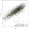 |
Fig. A.1 SFR-M⋆ relation for SDSS (this work) and CALIFA (Catalán-Torrecilla et al. 2015) star-forming galaxies. SFR-M⋆ fit to the running median for bins of 2000 objects obtained in this work for the complete sample (red dashed line) and for bins of 1000 objects in the range of z between 0.005 ≤ z< 0.05 (black solid line). Red dots represent the median values of SFR and M⋆ for CALIFA star-forming galaxies along five stellar mass bins for an equitable number of galaxies in each bin. The error bars in x- and y-axis represent the ±1σ confidence interval for stellar mass and SFR, respectively. |
Figure A.2 shows the size-M⋆ for SDSS and CALIFA star-forming galaxies. The linear fit to the running median of the size-M⋆ distribution for the complete sample (0.005 ≤ z ≤ 0.22) and the median values of size and M⋆ along five stellar mass bins for CALIFA star-forming galaxies are shown; equitable number of galaxies have been considered in each bin.
From the figures we can see that the median values of the SFR of CALIFA galaxies are representatives with the results obtained in this work for (nearby 0.005 ≤ z< 0.05) SDSS galaxies over the whole range of galaxy mass. Likewise, the median values of the galaxy size of CALIFA galaxies are visibly consistent with the SDSS galaxies distribution. Taking into account these results, we can consider CALIFA star-forming galaxies as representative of the SDSS star-forming galaxies sample used in this work.
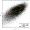 |
Fig. A.2 Size-M⋆ relation for SDSS (this work) and CALIFA (Catalán-Torrecilla et al. 2015) star-forming galaxies. Red solid line represents the linear fit to the running median for bins of 2000 objects in the SDSS star-forming galaxies. Red dots represent the median values of size and M⋆ for CALIFA star-forming galaxies along five stellar mass bins for an equitable number of galaxies in each bin. The error bars in x- and y-axis represent the ±1σ confidence interval for stellar mass and size, respectively. |
All Tables
Values of relevant parameters corresponding to the median (±1σ confidence interval) of the distribution for the star-forming galaxies in six redshift bins up to z = 0.22 in the total sample.
Values of aperture-corrected SFR corresponding to the median (±1σ confidence interval) of the distribution for the star-forming galaxies in twelve stellar mass bins in the total sample.
Values of stellar mass and aperture-corrected SFR per stellar mass and redshift bins corresponding to the median (±1σ confidence interval) of the distribution for the star-forming galaxies in the total sample.
All Figures
|
Fig. 1 [OIII] λ 5007/Hβ versus [NII] λ 6583/Hα diagnostic diagram (BPT) for the SDSS galaxies. Blue, green, and red points represent star-forming galaxies in the present work (209 276), composite galaxies (57 926), and AGN galaxies (19 392), respectively. The dashed line shows the Kewley et al. (2001) demarcation and the continuous line shows the Kauffmann et al. (2003a) curve. |
| In the text | |
|
Fig. 2 Density plots for the SDSS star-forming galaxies: i) left panel: the relation between log (M⋆/M⊙) and A(Hα); ii) central panel: the relation between log (SFR/M⊙ yr-1) and A(Hα), the inset plot shows the A(Hα)-log (sSFR/Gyr-1) relation; iii) right panel: the relation between EW(Hα) and A(Hα). The dashed lines represent the 1σ, 2σ, and 3σ contours. |
| In the text | |
|
Fig. 3 Relation between the SFR and M⋆ for star-forming galaxies. The red solid line and green dashed line represent the fit to the running median for bins of 2000 objects in this work and in the SDSS fibre, respectively. The red dotted line represents the linear fit to the running median for bins of 2000 objects in this work. The vertical black line shows the 1σ average dispersion (~0.3 dex). The inset plot shows the sSFR-M⋆ relation for our sample and the running median, for bins of 2000 objects, for the sSFR corrected for aperture (red solid line) and inside the SDSS fibre (green dashed line). |
| In the text | |
|
Fig. 4 Empirical SFR corrections (total – SDSS fibre) vs. M⋆ relation. Red, blue, green, magenta, orange, and gold lines represent the fit to the running median for bins of 1000 objects in six redshift bins up to z = 0.22 for a sample of star-forming galaxies. The numbers of star-forming galaxies in each redshift bin appear on the legend. The vertical black dotted line corresponds to the reference value at log (M⋆/M⊙) = 10. |
| In the text | |
|
Fig. 5 Relation between the SFR and M⋆ for SDSS star-forming galaxies, along three stellar mass bins for the whole mass range (8.5 ≤ log (M⋆/M⊙) ≤ 11.5) and for six redshift ranges in the range 0.005 ≤ z ≤ 0.22. The black solid line represents the fit to the running median for bins of 1000 objects in this work for each redshift range. Red dots represent the medians of SFR and M⋆ per stellar mass bin and redshift range. The error bars in x- and y-axis represent the ±1σ confidence interval for stellar mass and SFR, respectively. The symbol sizes increase with the number of objects contained in each mass range. |
| In the text | |
|
Fig. 6 Left panel: difference, Δlog (SFR), of total SFR provided by MPA-JHU (Brinchmann et al. 2004b; Salim et al. 2007) and our total empirical SFRThis work as a function of SFRThis work; right panel: difference of the total SFR derived using the Hopkins et al. (2003) aperture correction for the Hα flux and SFRThis work as a function SFRThis work. Upper numbers represent the number of high- (red points) and low-level (blue points) Hα emitting galaxies (colour–coded according to the EW(Hα) colour bar). The black dashed line indicates Δlog (SFR) = 0. |
| In the text | |
|
Fig. 7 SFRThis work−M⋆ relation for star-forming galaxies compared with previous theoretical and observational works. Comparison with observational studies: Panel a) SFR-M⋆ fits to the running median for bins of 2000 objects obtained in this work (red solid line) and from the SDSS fibre (brown dashed line), together with the values provided by MPA-JHU (blue dotted line), using the Hopkins et al. (2003) recipe (orange solid line), and from our refined method of Hopkins et al. (2003) recipe (orange dashed line). Panel b) Difference vs. M⋆ between SDSS fiber SFRs and SFRThis work and between observational studies and SFRThis work (colours as in upper left panel). Dotted line shows Δlog (SFR) = 0. Comparison with theoretical studies: Panel c) SFR-M⋆ fits to the running median for bins of 2000 objects obtained in this work (red solid line) and from the SDSS fibre (brown dashed line), together with the predictions from Sparre et al. (2015) (green dashed line) and Dutton et al. (2010; cyan dashed line). Panel d) Difference vs. M⋆ between SDSS fiber SFRs and SFRThis work and between theoretical predictions and SFRThis work (colours as in upper right panel). Dotted line shows Δlog (SFR) = 0. |
| In the text | |
|
Fig. A.1 SFR-M⋆ relation for SDSS (this work) and CALIFA (Catalán-Torrecilla et al. 2015) star-forming galaxies. SFR-M⋆ fit to the running median for bins of 2000 objects obtained in this work for the complete sample (red dashed line) and for bins of 1000 objects in the range of z between 0.005 ≤ z< 0.05 (black solid line). Red dots represent the median values of SFR and M⋆ for CALIFA star-forming galaxies along five stellar mass bins for an equitable number of galaxies in each bin. The error bars in x- and y-axis represent the ±1σ confidence interval for stellar mass and SFR, respectively. |
| In the text | |
|
Fig. A.2 Size-M⋆ relation for SDSS (this work) and CALIFA (Catalán-Torrecilla et al. 2015) star-forming galaxies. Red solid line represents the linear fit to the running median for bins of 2000 objects in the SDSS star-forming galaxies. Red dots represent the median values of size and M⋆ for CALIFA star-forming galaxies along five stellar mass bins for an equitable number of galaxies in each bin. The error bars in x- and y-axis represent the ±1σ confidence interval for stellar mass and size, respectively. |
| In the text | |
Current usage metrics show cumulative count of Article Views (full-text article views including HTML views, PDF and ePub downloads, according to the available data) and Abstracts Views on Vision4Press platform.
Data correspond to usage on the plateform after 2015. The current usage metrics is available 48-96 hours after online publication and is updated daily on week days.
Initial download of the metrics may take a while.