| Issue |
A&A
Volume 599, March 2017
|
|
|---|---|---|
| Article Number | A117 | |
| Number of page(s) | 15 | |
| Section | Interstellar and circumstellar matter | |
| DOI | https://doi.org/10.1051/0004-6361/201628507 | |
| Published online | 09 March 2017 | |
Absorption and scattering by interstellar dust in the silicon K-edge of GX 5-1
1 SRON Netherlands Institute for Space Research, Sorbonnelaan 2, 3584 CA Utrecht, The Netherlands
e-mail: This email address is being protected from spambots. You need JavaScript enabled to view it.
2 Leiden Observatory, Leiden University, PO Box 9513, 2300 RA Leiden, The Netherlands
3 Department of Earth and Space Science, Osaka University, 1-1 Machikaneyama, Toyonaka, 560-0043 Osaka, Japan
4 Debye Institute for Nanomaterials Science, Utrecht University, Universiteitsweg 99, 3584 CG Utrecht, The Netherlands
5 Astrophysikalisches Institut und Universitäts-Sternwarte (AIU), Schillergäßchen 2-3, 07745 Jena, Germany
6 Anton Pannekoek Astronomical Institute, University of Amsterdam, PO Box 94249, 1090 GE Amsterdam, The Netherlands
7 National Astronomical Observatory of Japan (NAOJ), 2-21-2 Osawa, Mitaka, 181-8588 Tokyo, Japan
Received: 14 March 2016
Accepted: 14 December 2016
Abstract
Context. We study the absorption and scattering of X-ray radiation by interstellar dust particles, which allows us to access the physical and chemical properties of dust. The interstellar dust composition is not well understood, especially on the densest sight lines of the Galactic plane. X-rays provide a powerful tool in this study.
Aims. We present newly acquired laboratory measurements of silicate compounds taken at the Soleil synchrotron facility in Paris using the Lucia beamline. The dust absorption profiles resulting from this campaign were used in this pilot study to model the absorption by interstellar dust along the line of sight of the low-mass X-ray binary GX 5-1.
Methods. The measured laboratory cross-sections were adapted for astrophysical data analysis and the resulting extinction profiles of the Si K-edge were implemented in the SPEX spectral fitting program. We derive the properties of the interstellar dust along the line of sight by fitting the Si K-edge seen in absorption in the spectrum of GX 5-1.
Results. We measured the hydrogen column density towards GX 5-1 to be 3.40 ± 0.1 × 1022 cm-2. The best fit of the silicon edge in the spectrum of GX 5-1 is obtained by a mixture of olivine and pyroxene. In this study, our modeling is limited to Si absorption by silicates with different Mg:Fe ratios. We obtained an abundance of silicon in dust of 4.0 ± 0.3 × 10⁻⁵ per H atom and a lower limit for total abundance, considering both gas and dust of >4.4 × 10⁻⁵ per H atom, which leads to a gas to dust ratio of >0.22. Furthermore, an enhanced scattering feature in the Si K-edge may suggest the presence of large particles along the line of sight.
Key words: astrochemistry / X-rays: binaries / dust, extinction / X-rays: individuals: GX 5-1
© ESO, 2017
1. Introduction
Cosmic silicates form an important component of the dust present in the interstellar medium (ISM). These silicate dust particles are thought to be mainly produced in oxygen-rich asymptotic giant branch (AGB) stars (e.g., Gail et al. 2009). Besides AGB stars, other sources such as novae, supernovae type II (Wooden et al. 1993; Rho et al. 2008, 2009), young stellar objects (Dwek & Scalo 1980), and red giant stars (Nittler et al. 1997) can produce silicate dust. Even dust formation in the ISM may occur in interstellar clouds (Jones & Nuth 2011). Although the amounts of dust contributed by these sources is still debated (Meikle et al. 2007; Jones & Nuth 2011), silicate dust is abundant in the ISM and can be found in many different stages of the life cycle of stars (Henning 2010). The physical and chemical composition of silicate dust has traditionally been studied at various wavelengths ranging from the radio to the UV and at different sight lines across the Galaxy (Draine & Li 2001; Dwek et al. 2004). However, there are still many open questions about, for instance, the chemical composition of silicates (Li & Draine 2001; Gail 2010), the production and destruction rate of dust (Jones et al. 1994, 1996), the amount of crystalline dust in the ISM (Kemper et al. 2004), and the particle size distribution and the shape of dust grains (e.g., Min et al. 2006, 2008; Voshchinnikov et al. 2006; Mutschke et al. 2009). Furthermore, it is not precisely known how the dust composition and the dust particle size distribution change in different regions throughout the Galaxy (Chiar & Tielens 2006; Min et al. 2007).
Elements such as C, O, Fe, Si, and Mg appear to be under-abundant in the cold phase of the ISM (Jenkins 2009; Savage & Sembach 1996). The abundances of these elements relative to hydrogen were found to be less than in the Sun, the Solar system, or in nearby stars (Draine 2003). The atoms, that appear to be missing, are thought to be locked up in dust. This is referred to as depletion from the gas phase, which is defined here as the ratio of the dust abundance to the total amount of a given element. A large fraction of C, O, Fe, Si, and Mg is therefore thought to be depleted and locked up in dust (Henning 2010; Savage & Sembach 1996; Jenkins 2009). Aside from carbon, which is mostly present in dust in graphite and polycyclic aromatic carbon (e.g., Zubko et al. 2004; Draine & Li 2007; Tielens 2008), these elements form the main constituents of cosmic silicates (Mathis 1998). Silicon in dust is mainly present in the ISM in the form of silicates, although it may also exist, in relatively small percentages, in the form of SiC: 0.1%, (Kemper et al. 2004), 9–12% (Min et al. 2007). Mg and Fe oxides are observed in stellar spectra (Posch et al. 2002; Henning et al. 1995), but there is no observational evidence for them in the diffuse ISM (Whittet et al. 1997; Chiar & Tielens 2006). However, these compounds have been isolated as stardust in Solar system meteorites (Anders & Zinner 1993).
An important property of interstellar dust is crystallinity. From observations of the 10 μm and 18 μm features, Kemper et al. (2004) concluded that along sight lines towards the Galactic center, only 1.1% (with a firm upper limit of 2.2%) of the total amount of silicate dust has a crystalline structure. On the other hand, some of the interstellar dust grains captured by the Stardust Interstellar Dust Collector (Westphal et al. 2014) showed a large fraction of crystalline material. The cores of these particles contained crystalline forsteritic olivine. Westphal et al. (2014) conclude that crystalline materials are probably preserved in the interiors of larger (>1μm) particles. Interestingly, dust is found to be in crystalline form at the start and at the end of the life cycle of stars, whereas very little crystalline dust appears to survive the harsh environment of the ISM. There are indications that the amount of crystalline dust depends on the environment. For instance, silicate dust in starburst galaxies appears in large fractions in crystalline form (Spoon et al. 2006; Kemper et al. 2011), probably reflecting freshly produced dust. Indeed, silicates in the ISM can be amorphous either because during the formation process the silicates condense as amorphous grains (Kemper et al. 2004; Jones et al. 2012) or the crystal structure is destroyed in the ISM by cosmic ray bombardments, UV/X-ray radiation, and supernova shock waves (Bringa et al. 2007). In the first case the silicates will have a non-stoichiometric composition and in the second case they will have the stoichiometry of the former crystal (Kemper et al. 2004). The dust features of amorphous dust are smoother than those of crystalline dust, which makes the determination of the structure and composition of the interstellar dust from spectral studies more difficult.
From X-ray observations of sight lines towards the Galactic plane and infrared observations towards the Galactic center, silicates were found to be Mg-rich rather than Fe-rich (Costantini et al. 2005, 2012; Lee et al. 2009; Min et al. 2007). However, Fe is heavily depleted (70−99%) and probably mostly locked up in dust grains (Wilms et al. 2000; Whittet 2003). It is not certain in which exact form Fe is incorporated into dust (Whittet et al. 1997; Chiar & Tielens 2006). Since the composition of certain silicates allows iron rich compounds, it is possible that some of the iron is locked up in these silicate grains. Another and possibly complementary scenario to preserve Fe in dust prescribes that Fe could be locked up in Glass with Embedded Metal and Sulfides (GEMS) of interstellar origin (e.g. Bradley 1994; Floss et al. 2006; Keller & Messenger 2013).
The abundances of most of the important metals decrease with distance from the Galactic plane, which can be described by a gradient with an average slope of 0.06 dex kpc-1 (Chen et al. 2003, and references therein). Although the ISM shows this general gradient, the ISM is also very patchy. The measurements of abundances show a large scatter as function of the Galactic radius, due to local influences of, for instance, supernova ejecta and infalling metal-poor gas onto the disk (Nittler 2005). The 10 μm feature provides information about the Si abundance in the Galaxy, which in turn can provide restrictions on the dust composition and possibly on the dust size distribution (Tielens et al. 1996). It is not precisely known how the dust distribution and the dust composition change relative to the environment. Simple dust size distributions, such as the Mathis-Rumpl-Nordsieck (MRN, Mathis et al. 1977) distribution, consisting of solid spherical dust particles, may not be sufficient to explain the observations towards dense regions of the Galaxy. Dust particles may be non-spherical and porous due to the formation processes of dust (Min et al. 2006, 2007; Chiar & Tielens 2006). Furthermore, Hoffman & Draine (2016) show the importance of incorporating non-spherical dust particles into X-ray scattering analyses.
X-ray observations provide a hitherto relatively unexplored but powerful probe of interstellar dust (Draine 2003; Lee et al. 2009; Costantini et al. 2012). The extinction features near the X-ray edges of O, Mg, Si, and Fe can be analyzed depending on the column density on the line of sight towards the source and the sensitivity of the detector. The X-ray Absorption Fine structures (XAFS) near the atomic absorption edges of elements provide a unique fingerprint of the dust. These XAFS have been observed in the X-ray spectra of astrophysical objects in data from XMM and Chandra (Lee et al. 2001; Ueda et al. 2005; Kaastra et al. 2009; de Vries & Costantini 2009; Pinto et al. 2010, 2013; Costantini et al. 2012; Valencic & Smith 2013). The X-rays provide important advantages compared to longer wavelengths and, in that way, provide an independent method to study silicate dust. The two most important advantages are that it is possible to measure the quantity of absorbing gas and dust simultaneously and to directly determine the composition of the dust. In particular, it is, in principle, possible to address the abundance, composition, stoichiometry, crystallinity, and size of interstellar silicates.
Bright X-ray binaries, distributed along the Galactic plane, can be used as background sources to probe the intervening dust and gas in ISM along the line of sight. In this way, a large range of column densities can be investigated and it is possible to analyze dust in various regions in the Galaxy. Dust in diffuse regions along the Galactic plane has been studied in the X-rays by Lee et al. (2009), Pinto et al. (2010, 2013), and Costantini et al. (2012) for several sight lines. The dense ISM has been less extensively studied in the X-rays. These dense environments (hydrogen column density >1 × 1022 cm-2) can be studied in the X-rays by observing the Mg and Si K-edge. In this paper we will focus in the Si K-edge.
The information on silicon in silicates of astronomical interest is very limited and sparse. The Si K-edge of some silicates has been measured by Li et al. (1995), Poe et al. (1997), for example, but most of these silicates cannot be used in astronomical studies because they also contain elements which are not abundant in the ISM. In this first study of the Si K-edge in astronomical data with a physically motivated model, we present a new set of laboratory measurements of Si K-edges of six silicate dust samples. The samples contain both crystalline and amorphous silicates. Further details about these samples are given in Sect. 3.1. The measurements are part of a large laboratory measurement campaign aimed at the characterization of interstellar dust analogs (Costantini & de Vries 2013).
We analyze the interstellar matter along the line of sight of X-ray binary GX 5-1 using models based on new laboratory measurements and discuss the properties and composition of the dust. The paper is structured in the following way: in Sect. 2, we explain the usage of XAFS to study interstellar dust. In Sect. 3, the data analysis of the laboratory samples is described. Section 4 shows the calculation of the extinction cross-section (absorption and scattering) of the samples. Section 5 describes the source GX 5-1. In Sect. 6, we fit the models to the spectrum of GX 5-1 and determine the best fit to the data using the samples from Sect. 3. We discuss our results in Sect. 7 and conclude in Sect. 8.
2. X-ray absorption edges
The modulations at the absorption edges of elements locked up in dust are called X-ray absorption fine structures (XAFS, Meurant 1983). XAFS are best understood in terms of the wave behavior of the photo-electron. These structures arise when an X-ray photon excites a core electron. The outwardly propagating photo-electron wave will be scattered by the neighboring atoms. From these atoms, new waves will emanate and will be superimposed on the wave function of the photo-electron. The wave function of the scattered photo-electron is therefore modified due to constructive and destructive interference. In this way, the absorption probability is modified in a unique manner, because it depends on the configuration of the neighboring atoms. These modulations can be used to determine the structure of the silicate dust in the ISM, because the modulations show unique features for different types of dust.
Samples.
3. Laboratory data analysis
3.1. The samples
We analyzed six samples of silicates. The compounds are presented in Table 1. Three of the samples were natural crystals, that is, two orthopyroxenes, one of them magnesium-rich (sample 4: enstatite, origin Kiloza, Tanzania), one with a higher iron content (sample 6: hypersthene, origin: Paul Island, Labrador), and one is an iron-rich olivine (sample 1: olivine, origin: Sri Lanka). See also Jaeger et al. (1998) and Olofsson et al. (2012) for infrared data of the enstatite and the olivine crystals.
The three other samples, that is, sample 2, sample 3 (which is the crystalline counterpart of sample 2), and sample 5, were synthesized for this analysis in laboratories at AIU Jena and Osaka University. The amorphous Mg0.9Fe0.1SiO3 sample has been synthesized by quenching of a melt according to the procedure described by Dorschner et al. (1995). The crystalline counterpart was obtained by slow cooling of silicate material produced under Ar atmosphere in an electric arc, similarly to that described for Mg/Fe oxides in Henning et al. (1995).
We were motivated in the choice of the sample by the almost absolute absence of XAFS measurements for silicates of astronomical interest. In order to produce laboratory analogs of interstellar dust silicates, four main criteria were considered:
-
The samples (or a mixture of these samples) should reflect theinterstellar dust silicates of “mean” cosmic composition.
-
The samples have an olivine or pyroxene stoichiometry.
-
The samples contain differences in the Mg:Fe ratio.
-
The sample set contains both amorphous and crystalline silicates.
The composition of the samples present in our study is chosen in such a way that mixtures of these samples can reflect the cosmic silicate mixture as described by Draine & Lee (1984). According to observations of 10 and 20μm absorption features in the infrared, the silicate dust mixture consists of an olivine and pyroxene stoichiometry (Kemper et al. 2004; Min et al. 2007). The dominating component seems to be silicates of an olivine stoichiometry (Kemper et al. 2004). Min et al. (2007) show that the stoichiometry lies in between that of olivine and pyroxene, which suggests a mixture of these two silicate types. Therefore, our sample set contains both pyroxenes and an olivine silicate. The samples show variations in the Mg:Fe ratio. These variations reflect the results from previous studies of interstellar dust. Kemper et al. (2004) infer from the observed stellar extinction that Mg/(Mg + Fe) ~ 0.5, whereas Min et al. (2007) conclude that Mg/(Mg + Fe) ~ 0.9. Silicates with a high magnesium fraction of Mg/(Mg + Fe) ~ 0.8 have been found in environments that show silicates with a crystalline structure, for example around evolved stars (Molster et al. 2002a,b,c; de Vries et al. 2010), in comets (Wooden et al. 1999; Messenger et al. 2005), and in disks around T Tauri stars (Olofsson et al. 2009). Therefore, our samples have ratios of Mg/(Mg+Fe) that vary between 0.5 and 0.9. The sample set also contains both amorphous and crystalline silicates.
Besides the two amorphous pyroxene samples present in this set, another highly suitable candidate would be an amorphous olivine, which is not present in this analysis. In general, amorphous olivine is difficult to synthesize, because this particular silicate crystallizes extremely quickly. A rapid-quenching technique is necessary to prevent the crystallization process. For compounds with a higher iron content, this technique may not be fast enough to prevent both phase separation and crystallization. Even at moderately high Fe contents, the silicates would show variations of the Mg:Fe ratio throughout the sample. These variations are problematic in the comparison with their crystalline counterpart. In the initial phase of this campaign, we indeed also analyzed the amorphous olivine, originally used in Dorschner et al. (1995). The inspection with the electron microscope revealed this particular sample to be both partially inhomogeneous in composition and contaminated by tungsten. This element has significant M-edges around the Si K-edge (i.e., the M1-M5 edges of tungsten fall in a range between 1809 and 2819 eV, where the Si K-edge is at 1839 eV). For these reasons, the amorphous olivine from Dorschner et al. (1995) was discarded at a very early stage of this campaign, as it was unsuitable for fluorescence measurements in the X-rays.
3.2. Analysis of laboratory data
Ideally one would like to measure the absorption of the samples directly in transmission through the sample, because this would resemble the situation in the ISM more closely. However, to measure the dust samples in transmission around the energy of the Si K-edge, we need optically thin samples, which implies a sample thickness of 1.0–0.5μm. This is impossible to obtain for practical reasons. In our analysis of the silicon K-edge we make use of optically thick samples (i.e., the sample is much thicker than the penetration depth) and therefore it is necessary to use a different technique with which the absorption can be derived. There are two processes that can be used in this case, which occur after the core electron is excited by an X-ray photon. The excited photo-electron leaves a core hole. This can be filled by an electron from a higher shell that falls into the vacancy. The excess energy can either be released as a fluorescent photon or another electron gets ejected. The latter is called the Auger effect (Meitner 1922). Depending on the attenuation of the signal, both effects can be used to derive the amount of absorption around the edge. Since the fluorescent signal of our measurements was strong enough, we used the fluorescent measurements of the Si Kα line in our analysis of the Si K-edge.
The absorption (given here by the absorption coefficient α(E)) can be derived from the fluorescent spectrum by dividing the fluorescent intensity (If) by the beam intensity (I0).  (1)The samples were analyzed at the Soleil synchrotron facility in Paris using the Lucia beamline. They were placed in the X-ray beam and the reflecting fluorescent signal was measured by four silicon drift diode detectors. The beam has an energy range of 0.8–8 keV. The energy source of the X-ray beam is an undulator, which creates a collimated beam. The beam is first focused by a spherical mirror and then passes two sets of planar mirrors that act as a lower pass filter. This procedure reduces the high-order contamination from the undulator and the thermal load received by the monochromator crystals. The monochromator crystals then rotate the beam and keep the exit beam at a constant height. There are five different crystals available. During our measurements, we made use of the KTP monochromatic crystals. In the energy range of 1280 to 2140 eV, the KTP monochromatic system has an energy resolution between 0.25 and 0.31 eV (Flank et al. 2006). The beam energy can be increased gradually (stepped by the resolution of the monochromator) in order to measure the absorption at the pre-edge (1800–1839 eV), the edge itself (at 1839 eV), and the post-edge (1839–2400 eV). The measurements were made with 0.5 eV energy spacing between measurements close to the edge. The added signal of the four silicon drift diode detectors yields the total fluorescent spectrum from the sample, from which the absorption coefficient α(E) can be derived using the beam intensity I0 as indicated in Eq. (1).
All six samples were stuck on two identical copper sample plates. The silicates were ground to a powder and pressed into a layer of indium foil, which made it possible for the samples to stick to the copper plates. Each sample was measured twice and therefore four measurements of each compound were obtained. This was done to avoid any dependence in the measurement on the position of the sample on the copper plate. The average of the four measurements is used in this analysis. The dispersion among the measurements is small; 3%.
The measurements of the samples were corrected for pile-up and saturation. Pile-up is caused by the detection of two photons instead of one at the same time on the detector. This can be seen on the detector as an extra fluorescent line at twice the energy of the expected fluorescent Kα line. This means that some of the intensity of the original line would be lost. To correct for this effect, we isolated both the silicon fluorescent line and the associated pile-up line from the fluorescent spectrum. The contribution of the pile-up line is then weighed and added to the original line. A comparison between the corrected and uncorrected data shows that the influence of pile-up in the sample is minimal (<1%).
As indicated by Eq. (1), the intensity of fluorescence is proportional to the absorption probability, but this is a slight oversimplification. The fluorescent light has to travel through the sample before it can be detected. On the way through the sample, the photons can be absorbed by the sample itself and the fluorescence intensity is attenuated. This effect is called saturation. This means that the measured fluorescent signal If is no longer proportional to the absorption coefficient. In our measurements, the samples were all placed at an angle θ = 45 °; therefore, the angular dependence can be neglected. Another advantage of positioning the sample in this way is that the beam and the detector are now at a 90 ° angle. Due to the polarisation of the radiation from the incident beam, the beam is greatly suppressed at this angle and almost no radiation from the beam can reach the detector directly. The measured fluorescence intensity divided by the intensity of the beam can now be expressed as: ![Mathematical equation: \begin{equation} \frac{I_{\rm f}}{I_0}=\epsilon_{f}\frac{\Omega}{4\pi}\frac{\alpha_{e}(E)}{\alpha_{\mathrm{tot}}(E)+\alpha_{\mathrm{tot}}(E_{\rm f})}[1-e^{{-[\alpha_{\mathrm{tot}}(E)+\alpha_{\mathrm{tot}}(E_{\rm f})}]x_n/\sin(\theta)}] \label{eq:flou1} . \end{equation}](/articles/aa/full_html/2017/03/aa28507-16/aa28507-16-eq37.png) (2)In this equation, ϵf is the fluorescence efficiency, xn/ sin(θ) is the effective optical path (where xn is the penetration depth into the sample and θ is the angle between the sample surface and the beam), Ω is the solid angle of the detector, Ef is the energy of the fluorescent X-ray photons, αe(E) is the absorption from the element of interest and αtot is the total absorption defined as: αtot = αe(E) + αb(E). αb(E) denotes the absorption from all other atoms and other edges of interest. For concentrated samples, αb(E) can become dominant and the XAFS will be damped by this saturation effect. In the ISM, the dust is very diluted, so saturation will not occur in real observations, but has to be corrected for in bulk matter.
(2)In this equation, ϵf is the fluorescence efficiency, xn/ sin(θ) is the effective optical path (where xn is the penetration depth into the sample and θ is the angle between the sample surface and the beam), Ω is the solid angle of the detector, Ef is the energy of the fluorescent X-ray photons, αe(E) is the absorption from the element of interest and αtot is the total absorption defined as: αtot = αe(E) + αb(E). αb(E) denotes the absorption from all other atoms and other edges of interest. For concentrated samples, αb(E) can become dominant and the XAFS will be damped by this saturation effect. In the ISM, the dust is very diluted, so saturation will not occur in real observations, but has to be corrected for in bulk matter.
In the case of a thick sample, the exponential term in Eq. (2) becomes small and can be ignored:  (3)The correction has been done using the FLUO software developed by Daniel Haskel. FLUO is part of the UWXAFS software (Stern et al. 1995). A detailed explanation of this correction can be found in Appendix A1. This routine uses tabulated absorption cross-sections to correct most of the distortion in order to recover the actual absorption coefficient. In comparison to the correction for pile-up, the correction of the absorption spectra for saturation is considerable as can be seen in Fig. 1.
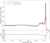 |
Fig. 1 Example of the difference between the sample corrected for saturation and the uncorrected measurement. Shown is sample 3, crystalline pyroxene. The lower panel shows the ratio of the corrected and uncorrected measurement. |
Figure 2 shows the amount of absorption, indicated by the cross-section (in arbitrary units), corrected for saturation and pile-up as a function of the energy of the silicon K-edge for all the samples. This figure shows the differences in the XANES for different compounds. The structure of olivine (sample 1), for example, shows a peak at 6.69 Å that is not observed in the pyroxene samples. There is also a clear difference between amorphous and crystalline samples. Indeed, the structures that are present between 6.70 and 6.66 Å in sample 3, for example, are washed out in the amorphous counterpart: sample 2.
4. Extinction cross-sections
We derived the amount of absorption of each sample in arbitrary units from the laboratory data. These measurements need to be converted to extinction cross-sections (in units Mb) in order to implement them into the AMOL model of the fitting routine SPEX (Kaastra et al. 1996) for further analysis. The total extinction cross-section can be calculated by using the Mie theory (Mie 1908). In order to do so, we first need to derive the optical constants of the samples. In this section, we explain the methods used to obtain the extinction cross-section of each sample.
4.1. Optical constants
When light travels through a material, it can be transmitted, absorbed, or scattered. The transmittance T is defined as the ratio of transmitted I and incident light I0. The amount of light that is absorbed or transmitted depends on the distance the light travels through the material and on the properties of the material. The transmittance is described by the Beer-Lambert law (Eq. (4)):  (4)In this equation, x is the depth of the radiation in the material and α is the extinction coefficient. The transmittance is also equivalent to e− x/l, where x is again the depth of the radiation into the material and l is the mean free path (e.g., the average distance travelled by a photon before it is absorbed). The extinction coefficient depends on the properties of the material and is independent of the distance x traveled through medium. However, α does depend on the wavelength of the incident light. It can be expressed as α = ρκλ, where ρ is the specific density of the material and κλ is the cross-section per unit mass. The Beer Lambert law is an approximation, assuming that the reflections at the surfaces of the material are negligible. In the X-rays, the contribution of reflection becomes very small.
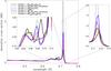 |
Fig. 2 Si K-edge of the six samples. The x-axis shows the energy in Å and the y-axis shows the amount of absorption indicated by the cross-section (in Mb per Si atom). |
In order to determine α from our measurements, we transform the absorption in arbitrary units obtained from the laboratory fluorescent measurements in Sect. 3, to a transmission spectrum. In order to do this, we use the tabulated values of the mean free path l provided by the Center for X-ray Optics at Lawrence Berkeley National laboratory2. These values of l are calculated at certain energies over a range from 10 to 30 000 eV. For each compound, the value of l can be determined over this range, taking the influence of all the possible absorption edges of the compound into account. Subsequently, Eq. (4) can be used to calculate the transmission T. We assume that x mimics an optically thin layer of dust to resemble the conditions in the ISM. Because α is independent of the depth the light travels into the material, we only need to make sure that we choose an optically thin value of x. Around 1839 eV, which is the position of the Si K-edge, l has a value of 3−5 μm (depending on the pre- or post edge side). This means that if we select a thickness of 0.5 μm (a value far below the penetration depth), the sample becomes optically thin and in that way we can mimic the conditions in the diffuse ISM. We now transform our absorption in arbitrary units from the laboratory data of Sect. 3 to transmission in arbitrary units. This laboratory transmission spectrum can be fitted to the transmission spectrum obtained from tabulated data. In this way, we can determine α as a function of energy (or wavelength) in detail around the edge, since  .
.
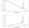 |
Fig. 3 Refractive index of sample 1 (olivine). The upper panel shows the real part of the refractive index (n) and the lower panel shows the imaginary part of the refractive index (k). |
In order to eventually determine the absolute extinction cross-section of the silicate we need to calculate its refractive index. The complex refractive index m is given by:  (5)where n and k are the real and imaginary part of m (also referred to as optical constants).
The imaginary part of the refractive index depends on the attenuation coefficient α:  (6)Since we already obtained α from the laboratory data in combination with the tabulated values, the imaginary part of the refractive index can be derived:
  (7)The real and imaginary part of the refractive index are not independent. They are related to each other by the Kramers-Kronig relations (Bohren 2010), in particular by:
 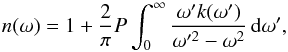 (8)where ω is the frequency at which the real refractive index is evaluated and P indicates that the Cauchy principle value is to be taken. The real part of the refractive index can be calculated using a numerical solution of the Kramers Kronig transforms. In this paper, we use a numerical method using the fast Fourier transform routines (FFT) as described in Bruzzoni et al. (2002). An example of the real and the imaginary part of the refractive index of sample 1 (olivine) is shown in Fig. 3.
4.2. Mie scattering calculations
When the optical constants n and k are calculated, we proceed with deriving the extinction cross-section for comparison with observational data. We use Mie theory to calculate the extinction efficiency (Qext(λ,a,θ)), calculated at each wavelength (λ) and particle size (a). The application of the Mie theory makes it possible to consider the contribution of both scattering and absorption to the cross-section. We assume a smooth dust distribution along the line of sight.
We use the grain-size distribution of MRN with a grain size interval of (a−,a+) is (0.005,0.25 μm). The MRN size distribution depends on the physical and chemical state of the dust grains. It is described by the following equation (in the case of silicate particles): 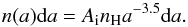 (9)In this equation, a is the particle size. A is the normalization constant, which depends on the type of dust. In the case of silicate (relevant in this paper): Asil = 7.8 × 10⁻²⁶ cm2.5 (H−atom)-1 (Draine & Lee 1984). n(a) is the number of grains and nH is the number density of H nuclei (in both atoms and molecules).
One of the main advantages of using a MRN distribution is the simplicity of the model, which prevents the introduction of many free parameters. We can now calculate the extinction cross-section Cext by applying the Mie theory (Mie 1908). We use the MIEV0 code (Wiscombe 1980), which needs m and X, where  , as input and returns the extinction extinction cross-section Cext.
To obtain the total scattering cross-section per wavelength unit (σext(λ)), we need to integrate over the particle size distribution. 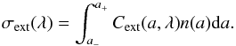 (10)To make the extinction cross-sections of the compounds compatible with the Verner cross-sections used by SPEX, we need to subtract the underlying continuum of the Henke tables (Henke et al. 1993). We remove the slope of the pre and post-edge by subtracting a smooth continuum in an energy range of 1.7–2.4 keV, which does not contain the edge. The result for sample 1 (olivine) is shown in Fig. 4. The continua have been calculated in the same way as the edges, but in this case the atomic edge jump was taken out of the cross-section. We then calculate the extinction cross-section in the same way as is described above, to obtain the continuum without the edge. To remove the continuum of the extinction profile, we subtract the continua without edges. This subtraction, which was done over the full energy range, puts the cross-section of the pre-edge at zero and therefore the scattering feature before the edge obtains a negative value. We then implement the models in SPEX. During the fitting, the continuum is naturally given by the X-ray continuum emission of the source.
A side note has to be made that SPEX fits the edges to the Verner tables instead of Henke. This means that there is a small discrepancy between the two parametrizations of approximately 2–5 percent around the silicon edge (J. Wilms, priv. comm.). This is well within the limit of precision that we can achieve from observations.
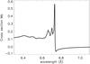 |
Fig. 4 Model of the Si K-edge of olivine (sample 1) as implemented in SPEX, without the continuum of the extinction profile. The cross-section in Mb is given per Si-atom. |
5. GX 5-1
As a first test of these new samples, we apply the new models to the source GX 5-1, which serves as a background source to observe the intervening gas and dust along the line of sight. GX 5-1 is a bright low-mass X-ray binary at (l,b) = (5.077,−1.019). Christian & Swank (1997) estimated distance to GX 5-1 to be 9 kpc. However, this distance may be regarded as an upper limit and the actual distance could be up to 30% (or 2.7 kpc) less, because the luminosity derived from the disk model used in their analysis exceeds the Eddington limit for accretion of either hydrogen or helium. GX 5-1 has been observed multiple times, for instance by Einstein (Christian & Swank 1997; Giacconi et al. 1979), as well as ROSAT, using the Position Sensitive Proportional Counter (Predehl & Schmitt 1995), and there are several observations by Chandra. In this work we use observations of the high-resolution spectrum of GX 5-1 collected by the HETG instrument on board Chandra. The Galactic coordinates combined with the distance indicate that GX5-1 is located near the Galactic center (assuming a distance towards the Galactic center of 8.5 kpc). Due to the uncertainty in the distance of GX 5-1, the source may either be in front, behind of embedded in the Galactic center region (Smith et al. 2006). The proximity to this region enables us to probe the dust and gas along one of the densest sight lines of the Galaxy. From CO emission observations towards the line of sight of GX 5-1 (observed by Dame et al. 2001), Smith et al. (2006) concluded that there are three dense regions along the line of sight, namely the 3 kpc spiral arm, the Giant Molecular Ring and the Galactic center. The three regions are at distances of 5.1, 4.7, and 8.5 kpc, respectively (Smith et al. 2006). The Giant Molecular Ring is assumed to be a region with a high molecular cloud density, which can be found approximately half way between the Sun and the Galactic center. All these regions may provide a contribution to the observed dust along the line of sight. The observation in the analysis of this paper therefore consists of a mixture of dust and gas in these regions.
6. Data analysis of GX 5-1
The spectrum of GX 5-1 has been measured by the HETG instrument of the Chandra space telescope. This instrument contains two gratings: HEG and MEG with a resolution of 0.012 Å and 0.023 Å (full width at half maximum), respectively (Canizares et al. 2005). The energy resolution of our models is therefore well within the resolution of the Chandra Space Telescope HETG detector. There are multiple observations of GX 5-1 available in the Chandra Transmission Gratings Catalog and Archive3, but only the observations in TE mode could be used to observe the Si K-edge (OBSID 716). This edge is not readily visible in the CC-mode, where it is filled up by the bright scattering halo radiation of the source. The edge has a slight smear as well as different optical depth. This effect is particularly evident in the CC mode, where the two arms of the grating are now compressed into one dimension, together with the scattering halo image (N. Schulz, priv. comm.)4.
GX 5-1 is the second brightest persistent X-ray source after the Crab Nebula (Smith et al. 2006). Due to the brightness of the source (with a flux of F0.5−2 keV = 4.7 ± 0.8 × 10⁻¹⁰ erg cm-2 s-1 and F2−10 keV = 2.1 ± 0.6 × 10⁻⁸ erg cm-2 s-1), the Chandra observation suffers from pile-up. This effect is dramatic in the MEG data, but also has an effect on the HEG grating. We, therefore, cannot use the MEG grating and need to ignore the HEG data below 4.0 Å. However, in this observation, GX 5-1 was also observed using both a short exposure of 0.2385 ks and a long exposure of 8.9123 ks. This is not a standard mode, but was especially constructed to evaluate the pile-up in the long exposure. The spectrum with an exposure time of 0.2385 ks does not suffer from pile-up due to the short exposure time per frame in the TE mode and can therefore be used to determine both the continuum and the hydrogen column density of the source.
Figure 5 shows the broad band spectrum of GX 5-1. The spectrum shows the presence of a strong Si K-edge at 6.7 Å superimposed on a strongly rising continuum towards shorter wavelength. The Si K-edge shows a strong transition with clear absorption structure at shorter wavelength, which is the tell-tale signature of solid-state absorption and an anomalous dispersion peak at the long wavelength, which reveals the presence of large grains (Van de Hulst 1958).
6.1. Continuum and neutral absorption
Before we can calculate the mixture of dust that best fits the data of GX 5-1, we need to determine the column density of hydrogen (NH) towards GX 5-1 and the underlying continuum of the source. Earlier research of Predehl & Schmitt (1995) using data from the ROSAT satellite shows that the value of the column density ranges between 2.78 and 3.48 × 1022 cm-2 depending on the continuum model. The disadvantage of the ROSAT data is that it only covers the lower-energy side (with 2 keV as the highest energy available, Trümper 1982) of the spectrum and therefore prevents the fitting of the hard X-ray energy side. This made it hard to predict which model would fit the spectrum the best and in that way influenced the value of NH. Other more recent measurements of the value of the column density were taken by Ueda et al. (2005); 2.8 × 1022 cm-2, based on fits on the same Chandra HETG data used in this analysis and Asai et al. (2000); 3.07 ± 0.04 × 1022 cm-2 (using ASCA archival data).
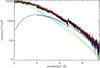 |
Fig. 5 Continuum of GX 5-1. Data from the HEG short exposure, MEG short exposure, and HEG long exposure (OBSID 716) were used to fit the continuum. The resulting fit to each of the three data sets is shown by a red line. The model consists of two absorbed black bodies. The two black bodies in the model are represented in the figure by the green and blue lines. For clarity, only the black body models of the HEG grating (both long and short exposure) are shown and the MEG data has been omitted in the figure, therefore each black body model shows two curves. |
The short Chandra HETG exposure does not suffer from pile-up and contains both the soft and the hard X-ray tail of the spectrum, therefore it can be used to derive the continuum and the NH for this analysis. The spectrum is best modelled by two black body curves using the bb model in SPEX. The spectrum is absorbed by a cold absorbing neutral gas model, simulated by the HOT model in SPEX. The temperature of this gas is frozen to a value of kT = 5 × 10⁻⁴ keV, in order to mimic a neutral cold gas. HEG and MEG spectra of the short exposure are fitted simultaneously with this model. The best fit for the continuum and the NH is shown in Fig. 5 and Table 2. It is necessary to constrain the NH well on the small wavelength ranges that are used in the following part of the analysis. In this way, the continuum is frozen and cannot affect the results of the dust measurements (see Sect. 6.2). Therefore, we use the HEG data of the long exposure to further constrain the column density. In the short exposure, we ignore the data close to the edge (6.2–7.2 Å), because the long exposure provides a much more accurate measurement of this part of the spectrum. In this way, the fit will not be biased by the lower signal-to-noise in the short exposure in this region. When we fit the model to the data, we obtain a good fit to the data with C2/ν = 1.16. For now, we only take cold gas into account to fit the continuum spectrum. This resulted in a column density of 3.40 ± 0.1 × 1022 cm-2 (see Fig. 5 and Table 2). All the fits in this paper generated by SPEX are using C-statistics (Cash 1979) as an alternative to χ2-statistics. C-statistics may be used regardless of the number of counts per bin, so in this way we can use bins with a low count rate in the spectral fitting5. Errors given on parameters are 1σ errors.
Broad band modelling of the source using HEG and MEG data from Chandra HETG.
6.2. Fit to Chandra ACIS HETG data of the silicon edge
After obtaining the NH value, we fit the dust models of the six dust samples to the Chandra HETG data. The shape of the continuum is fixed for now, to avoid any dependence of the fit on the continuum. The column density used for this fit is the NH derived in Sect. 6.1 and can vary in a range of 1σ from this value. To rule out any other dependence, we only use the data in a range around the edge: 6−9 Å. In this way we include the more extended XAFS features as well as part of the continuum in order to fit the pre and post edge to the data. The depletion values and ranges that were assumed for the cold gas component are listed in Table 3. Furthermore, SPEX uses protosolar abundances for the gas phase that are taken from Lodders & Palme (2009).
Depletion ranges used in the spectral fitting.
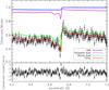 |
Fig. 6 Fit to the spectrum of GX 5-1 is shown in red. The contribution of the continuum is divided out. The other lines show the contribution of the absorbing components to the transmission. The purple line shows the contribution of pyroxene (sample 5), the green line the contribution of olivine (sample 1), and the blue line the contribution of gas. The lower panel shows the model residuals of the fit in terms of the standard deviation, σ. |
The SPEX routine AMOL can fit a dust mixture consisting of four different types of dust at the same time. Therefore, we test all possible configurations of the dust species and compare all the outcomes. We follow the same method as described in Costantini et al. (2012), where the total number of fits n is given by n = nedge ! (4 ! (nedge−4) !) and nedge is the number of available edge profiles.
In Fig. 6 we show the results of a fit of the SPEX model to the observed spectrum of GX 5-1. The best fit is shown by the red line. The mixture that fits the data best consists mainly of crystalline olivine (sample 1, green line) and a smaller contribution of amorphous pyroxene (sample 5, purple line) and neutral gas (blue line).
The reduced C2 value of the best fit is 1.05. We find that most dust mixtures that contain olivine fit the edge well and when pyroxene, with a high concentration of iron, is added to the fit, we obtain even better fits. When olivine is left out of the fit, the reduced C2 values increase from 1.05 to values of approximately 2. From our fitting procedure, we conclude that the dust mixture consists of 86 ± 7% olivine dust and 14 ± 2% pyroxene dust.
We calculated the dust abundances of silicon, oxygen, magnesium, and iron to be respectively 4.0 ± 0.3 × 10⁻⁵ per H atom, 17 ± 1 × 10⁻⁵ per H atom, 6.1 ± 0.3 × 10⁻⁵ per H atom, and 1.7 ± 0.1 × 10⁻⁵ per H atom. Unfortunately, the depletion hits the higher limit of the ranges set in Table 3. These ranges were set in order to keep the fit within reasonable depletion values. For this reason, we can only give upper limits to the depletion values we found, which are for O: <0.23, for Mg: <0.97, for Si: <0.87 and for Fe: <0.76. Table 4 lists the total column density, the depletion values, dust abundances, total abundances (including both gas and dust), and solar abundances for all the elements mentioned above. The total abundances can only be given as lower limits, since we can only put a lower limit on the gas abundance due to the upper limits on the depletion values. From our best fitting dust mixture, the total abundance of silicon along the line of sight towards GX 5-1 can be calculated using the column density of the best fit and the total amount of silicon atoms in both gas and solid phase. The resulting abundance is: >4.4 × 10⁻⁵ per H atom. The gas to dust ratio of silicon is 0.22.
Abundances and depletions.
Unconstrained silicon: abundances and depletions.
6.3. Hot ionized gas on the line of sight in the Si K-edge region?
Hot ionized gas along the line of sight might influence the silicon edge. In the energy range of the edge, we may observe absorption lines of this hot gas that may influence the shape of the silicon absorption edge. It may also be possible that this hot gas is intrinsic to the source. To be certain that this is not the case, we fitted the edge again as described above, but this time we add a slab of hot gas along the line of sight to our model. The lower and upper limits of the gas temperature are based upon the ionization fractions of neon by Yao & Wang (2005) and Yao et al. (2006). They observed hot gas in the ISM and compare the observed lines to ionization fractions for O, Ne, and Fe to determine the temperature of the gas. In this paper, we use the NeIX line to set the lower and upper limit of the hot gas (0.08–2.7 keV). At these temperatures of the hot gas, helium-like transitions of Si can occur at 6.69 and 6.65 Å. These lines can create additional features in the Si K-edge, so we fit the edge again with SPEX including an extra HOT model to model the hot gas. We do not detect any ionized gas along the line of sight towards GX 5-1. The gas temperature of the hot model hits the set limit of 0.08 keV, which is too cold to form any absorption lines near the silicon K-edge. Any ionized gas is therefore not likely to contaminate the Si K-edge in this data set.
7. Discussion
7.1. Abundances towards GX 5-1
7.1.1. Si abundance
In Sect. 6.2 we find that the abundance of silicon in dust is 4.0 ± 0.3 × 10⁻⁵ per H atom. We can compare this result to observations at infrared wavelengths in the solar neighborhood and towards the Galactic center. The 10 and 20μm lines of the Si-O bending and stretching modes were observed in order to measure the silicon abundances. We derived these abundances using the results from Aitken & Roche (1984), Roche & Aitken (1985), and Tielens et al. (1996). The silicon abundance was derived in two different regions of the Galaxy, namely the local solar neighborhood and a region close to the Galactic center. In the local solar neighbourhood towards sight lines of bright nearby Wolf-Rayet stars the abundance of silicon in dust can be derived, resulting in a value of 5.2 ± 1.8 × 10⁻⁵ per H atom (Roche & Aitken 1984; Tielens et al. 1996). Measuring the Si abundance towards the Galactic center from the 10 μm absorption may be challenging. The abundances depend on an estimate of the visual extinction (AV) derived from the NH/AV ratio for the local Solar neighborhood from UV studies of the atomic and molecular hydrogen column densities (Bohlin et al. 1978), and this procedure may be more uncertain towards the Galactic center (Tielens et al. 1996). The silicon abundance may therefore suffer from additional uncertainty. The same analysis has also been carried out for sight lines towards the Galactic center (Tielens et al. 1996; Aitken & Roche 1984). Towards the sight line of a cluster of compact infrared sources 2 pc away from the Galactic center (Roche & Aitken 1985), the silicon abundance in dust was derived, resulting in a value of 3.0 ± 1.8 × 10⁻⁵ per H atom. This is almost half of the value of the dust abundance measured in the local solar neighborhood. This discrepancy is not well understood. An explanation could be that the difference in abundance is caused by presence of large particles (grain sizes >3μm) near the Galactic center, which, however, is difficult to observe in the infrared (Tielens et al. 1996).
The abundance of silicon in dust found in Sect. 6.2, falls in between the two results for the local ISM and the Galactic center obtained in the infrared. When we consider the total abundance (including the contribution from gas), this increases the total abundance to >4.4 × 10⁻⁵ per H atom, which would correspond more with values found in the local solar neighborhood than those of the Galactic center. When we compare the total abundance of silicon to the protosolar abundance from Lodders & Palme (2009), we find only a small deviation from the solar abundance, namely: AZ/A⊙> 1.14. Furthermore, since we probe the inner regions of the Galaxy, it is not unrealistic to encounter a total abundance of silicon larger than solar along the line of sight.
Another comparison can be made using the observations towards the low-mass X-ray binaries 4U 1820-30 (Costantini et al. 2012) and X Per (Valencic & Smith 2013). In contrast to GX 5-1, these lines of sight probe the diffuse ISM. Towards 4U 1820-30 the abundance is  and towards X Per is 3.6 ± 0.5 × 10⁻⁵ per H atom. The lower limit of the Si abundance found in our analysis does, therefore, agree with the results of the diffuse ISM. The actual value of the Si abundance might indeed be higher than the average Si abundance in the diffuse ISM, but we need upper limits to the abundances to confirm this by obtaining better estimates on the depletion values. This may be obtained by releasing the range on the silicon depletion, which is discussed in Sect. 7.1.2.
7.1.2. Depletion of silicon
Since the depletion value of silicon reached the lower limit, we also show the results of a fit without restrictions on the silicon depletion values. These results are shown in Table 5 and Fig. 7. By releasing the range on the silicon depletion, we get a better impression of the total abundance of silicon.
Since we are currently analyzing the K-edge of silicon, we are able to directly measure the abundance of depletion in both gas and dust of this element only. The abundances of other elements are derived indirectly from the model and their depletion values should thus be kept in a limited range. We performed the fit again, leaving the depletion of Si free to vary without predefined boundaries. In this case, we obtain a depletion value of 0.68 ± 0.12. This value is within the 1 sigma error consistent with the value in Table 4. The best fit in Fig. 7 shows the same samples as the best fit in Sect. 6.2 (namely sample 1 olivine and sample 5 pyroxene), but there is a relatively larger contribution of gas, at the expense of the amorphous pyroxene contribution. As a consequence, the dust abundance value is reduced. Both AZ and AZ/A⊙ are now constrained. AZ/A⊙ seems to show a clearer overabundance of Si. This is expected in environments close to the Galactic center. The value of the total silicon abundance, AZ = 5.0 ± 0.5 × 10⁻⁵ per H atom, is comparable with values found in the local solar neighborhood. The differences between Ntot, the depletion, AZ,  , and AZ/A⊙ in Table 4 and Table 5 are small in the case of the other elements: Fe, Mg, and O. This is expected, because the range on the depletion ranges of these elements were kept the same in both fits. The number of fit parameters did not change, nor did the quality of the fit. Therefore, the reduced C2 value of the fit remains at 1.05. However, since the depletion of silicon in dense environments is expected to be higher than 0.68 ± 0.12, as is shown in previous studies (Wilms et al. 2000; Jenkins 2009; Costantini et al. 2012), we conservatively keep the silicon depletion constrained by the limits in Table 4 in further analysis of the edge.
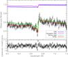 |
Fig. 7 Upper panel: a fit of the Si K-edge, where the depletion of silicon is left as a free parameter without boundary values. The best fitting mixture consist of the same compounds as the fit in Sect. 6.2: sample 1 (crystalline olivine) and sample 5 (amorphous pyroxene). Lower panel: model residuals of the fit in terms of the standard deviation, σ. |
7.1.3. Other abundances: oxygen, magnesium, and iron
The abundances of the other elements are listed in Table 4. Silicon and oxygen show abundances comparable to the solar values of Lodders & Palme (2009). Magnesium and iron show a deviation from protosolar abundances. The abundances in the Galaxy follow a gradient of increasing abundance towards the plane of the Galaxy. In the inner regions of the Galaxy, the abundances of the elements are expected to be supersolar (see Sect. 1). Most of the lower limits on the abundances correspond to values found in studies of the diffuse ISM (Pinto et al. 2010; Costantini et al. 2012; Valencic & Smith 2013). Since we can only show lower limits, we expect the true abundance to be higher, which would correspond with the expected increase of abundances toward the region around the Galactic center. The abundance of magnesium is supersolar, whereas the iron abundance in our result is subsolar. The missing iron can be present in other forms of dust. A possibility could be that iron is included in metallic form in GEMS (Bradley 1994).
7.2. Comparison to iron-poor, amorphous, and crystalline dust
An insightful way to compare the best fitting mixture to all the other possible mixtures is by comparing the best fitting mixtures with the two distinct variations in the samples: iron-rich/iron-poor and crystalline/amorphous. We select three different types of mixtures that we compare to the best fitting mixture, namely an iron-poor mixture (since the best-fitting mixture is iron-rich), a mixture of amorphous compounds and a mixture of crystalline compounds. The results are shown in Fig. 8.
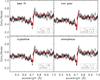 |
Fig. 8 Comparison of the best fit (upper left window) with iron-poor dust mixtures, strictly crystalline mixtures, and amorphous mixtures. |
The fit that resembles the best fit the most, is the fit containing only crystalline compounds. This fit consists only of olivine, which is the compound that is dominating the best fit of Sect. 6.2. The fit improves when amorphous pyroxene is added. The different compounds show a strong variation in the absorption at wavelengths of less than 6.6 Å relative to the K-edge at 6.7 Å Fig. B.1. This difference causes the poor fits for amorphous or iron samples (Fig. 8). The resulting fits in Fig. 8 strongly depend on the amount of silicon atoms available in the solid state, which is restricted by the column density NH. As can be observed in Fig. B.1 not every edge of the samples is equally deep. Models that produce deep absorption features around the edge, demand the presence of a certain amount of silicon in dust present along the line of sight. The amount of silicon present constrains the best fitting model in this way. The result of fitting a sample to the edge that requires a larger amount of silicon along the line of sight can be observed in the iron poor and amorphous windows of Fig. 8. Here the edge of the models is too deep and the post edge (which is here the part below 6.6 Å) never recovers to fit the data in this part of the plot. The amount of Si along the line of sight can be enhanced if the NH increases. When we enhance NH to values >5 × 1022 cm-2 the iron poor and amorphous models start to fit the edge, but such a NH is too high for GX 5-1. A well-determined column density of hydrogen is, for this reason, of great importance.
The best fit in Sect. 6.2 shows that we detect 86 ± 7% of crystalline olivine dust and only 14 ± 2% of amorphous pyroxene dust. This result gives us a relatively high crystallinity, that is, 79−93% of the total amount of dust has a crystalline structure. This somewhat surprising result may be in line with recent results from the Stardust mission (Westphal et al. 2014) and detection of dust in external galaxies (Spoon et al. 2006; Kemper et al. 2011), which suggests that crystalline dust may be more abundant than expected (Kemper et al. 2004); see Sect. 1. Limitations on this result are addressed in Sect. 7.4.
7.3. Comparison with dust compositions along other sight lines
We can compare the best fitting dust mixture to results from studies of dust in the infrared and X-ray studies of dust in the diffuse ISM. The bending and stretching modes of silicon in the infrared are often attributed to a mixture of enstatite and olivine (Kemper et al. 2004; Chiar & Tielens 2006). More detailed studies on the dust composition can be acquired from X-ray studies. Studies of the diffuse ISM show variation of the composition of the ISM along different lines of sight (Lee et al. 2009; Pinto et al. 2010; Costantini et al. 2012; Valencic & Smith 2013). From studies of the Fe L and O K-edge, Pinto et al. (2010) concluded that the dust composition of interstellar dust is probably chemically inhomogeneous, since they found indications for iron rich silicates toward X-ray binary GS 1826-238. Lee et al. (2009), on the contrary, find that Fe oxides provide a better fit to the data of Cyg X-1. Costantini et al. (2012) concluded from an analysis of the oxygen K-edge and the iron L-edge of the source 4U 1820-30, that GEMS could possibly be present along this line of sight. Their best fitting mixture, is a mixture of enstatite and metallic iron, which suggests that the dust in this region mostly consists of enstatite with metallic inclusions.
Along the line of sight toward X Per, a dust mixture of MgSiO3 and iron bearing silicates such as Mg1.6Fe0.4SiO4 provide a good fit to the observed spectrum (Valencic & Smith 2013). They conclude that although MgSiO3 is the dominating compound, the fit improves when iron-bearing silicates are included. The best fitting dust mixture in this study consists of the compounds that contain the largest amount of iron available in our set of compounds. Compared to the amount of magnesium present in these samples however, we can still consider this dust mixture as relatively iron poor. This is also reflected in the abundances of iron and magnesium of the best fit.
7.4. Limiting factors in the analysis of the Si K-edge
The modeling of a photo-electric edge such as the Si K-edge involves many components, which may influence the resulting shape of the edge. This requires a careful analysis of the resulting best-fit. This paragraph provides more insight into the quality of the fits and the limitations that arise in the analysis.
The quality of the fit depends in the first place on the resolution of the instrument. The observations used in this analysis were observed with the HEG grating of the Chandra X-ray telescope. This grating provides us with the best resolution currently available close to the Si K-edge. The bright source provides us with a high flux near the Si K-edge and the edge falls well within the range of the grating, where the effective area of the instrument is large. The minimum S/N per bin near the Si K-edge is 20, which is sufficient for the study.
Additionally, the accuracy of the results depends on the degrees of freedom of the fit and, of course, on the completeness of the dust models. SPEX allows a maximum input of four different dust components in the same fit. If we examine the output of the fits for all the possible dust mixtures, most of the resulting fits contain two dust components with negligible contribution from the other two possible components. In almost all the fits, one of the dust components dominates. The contribution of the second component is, in most cases, no more than 20% and in two cases there is a contribution of a third component, which is never more than 1−2%. When we analyze the fits that are within 3 sigma of the best-fit values presented in Sect. 6.2, the dominating component in these fits is crystalline olivine. Interestingly, all the dust mixtures where olivine is not included do not fall within 3 sigma of our best fit and can be ruled out.
Our set of models is sufficient for a pilot study of the Si K-edge, but should be expanded for further analysis. The main limiting factor in this analysis is the absence of an amorphous olivine model as a counterpart to the crystalline olivine model (see Sect. 3.1). We note that the crystalline counterpart cannot be taken as a proxy for the amorphous one. As an example, see the profiles of pyroxenes in amorphous and crystalline form in Fig. 2. The sharp features of the XAFS in the observation of GX 5-1 are indicative of a crystalline structure (Fig. 2). However, if the shape of the amorphous olivine would follow that of a crystalline counterpart albeit less sharp, the fit may allow the presence of more amorphous olivine. At the moment we are unable to test this (see the discussion in Sect. 3.1). Therefore, we conclude that the interesting possibility of a high fraction of crystalline dust along this line of sight must be further verified.
Another limitation in our analysis could be the Mg:Fe ratio in our samples. The resulting abundances and depletion values in our analysis depend strongly on the best-fitting dust mixture. The silicates in our sample are mainly olivines and pyroxenes with different Mg:Fe ratios. All the samples are relatively iron poor with a maximum Fe contribution of Mg/(Mg+Fe) of 0.6 and although there are indications that interstellar and circumstellar may indeed be iron poor (Molster et al. 2002a,b,c; Chiar & Tielens 2006; Blommaert et al. 2014), it would be beneficial to include silicates with a higher iron content.
In order to better constrain the depletion values, it is necessary to expand the fit to a broader wavelength range and incorporate multiple edges in the analysis depending on the observed NH. In the case of GX 5-1, iron cannot be directly observed. The NH is not high enough to imprint a significant Fe K-edge. On the lower energy side, interstellar absorption suppresses the Fe L-edges at ~0.7 keV and the O K-edge at 0.543 keV. The iron abundance in silicates can therefore only be inferred from the best fitting dust mixture. Finally, the Mg K-edge in GX 5-1 suffers from a lower signal to noise ratio with respect to the Si K-edge, mainly because of the relatively high column density value. However, the Mg K-edge can in principle help significantly in breaking model degeneracies.
7.5. Scattering and particle size distributions
We use a MRN distribution to describe the particle size distribution. The distribution with particles sizes ranging between 0.005 μm and 0.25 μm implies that most of the mass is in the large particles, while most of the surface area is in the small particles. MRN offers a simple parameterization, useful in this study. It is beyond the scope of this paper to test more sophisticated models such as Weingartner & Draine (2001) and Zubko et al. (2004). We note, however, that these size distributions have a maximum size cutoff around 0.25 μm and the silicate-type distributions do not differ dramatically from one another.
In Fig. 6, it can be observed that there is a feature between 6.8 Å and the edge at 6.7 Å. The MRN distribution predicts a large amount of small particles in our models. These particles do not add significantly to the scattering features of the extinction profiles. The model does not fit the data in the area around 6.7 Å well, which may indicate the presence of larger particles along the line of sight than present in our model (Van de Hulst 1958). This section therefore contains an investigation of the effect of the particle size distribution and focuses, in particular, on the presence of particles larger than 0.25 μm. In order to model the enhancement of the scattering peak around 6.7 Å, we introduce a range of particle sizes: 0.05−0.5 μm. The effect of a change in the size distribution is shown in Fig. 9. The olivine Si K-edge with a MRN distribution with particle sizes of 0.005−0.25 μm is shown in red and in blue the same edge is shown but now with a MRN size distribution that has a particle range of 0.05−0.5 μm.
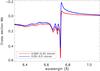 |
Fig. 9 Effect of a change in the size distribution on the extinction. The olivine Si K-edge with a MRN distribution with particle sizes of 0.005−0.25 μm microns is shown in red. The blue line shows the same edge, but now the particle sizes range between 0.05 and 0.5 μm. |
The edge is fitted again with models of the same compounds, that contain the new particle distribution. We use the same parameters as in the first fit in Sect. 6.2. The results are shown in Fig. 10. The reduced C2 value of the best fit is: 1.08. There is a small contribution (of less than 2% of the total amount of dust) of hypersthene (sample 6) in this fit in addition to amorphous pyroxene (sample 5) and crystalline olivine (sample 1). The contribution is so small that it does not significantly change any of the results derived above. The silicon abundance remains at 4.0 ± 0.4 × 10⁻⁵ per H atom. The scattering feature before the edge is better fitted using a model with larger particles, which leads to the possibility of the presence of particles larger than 0.25 μm. It is possible that in environments such as the Galactic center region we observe a substantial amount of particles larger than 0.25 μm (Ossenkopf et al. 1992; Ormel et al. 2009, 2011). In our analysis, we assume that the dust particles are solid spheres, while it is more likely that large particles in dense environments are grown by coagulation of dust particles (Jura 1980). Porous dust particles show an enhanced extinction profile when compared to solid particles of the same mass due to their larger surface area. Solid particles are too massive to be abundant enough to cause the enhanced scattering. Another indicator that dust particles are non-spherical is the observation of polarized starlight. Spheroidal grain models are able to reproduce these observations (Kim & Martin 1995; Draine 2009) and allow for larger particles in the size distribution (Draine 2009). The effects of large porous grains in X-rays have also been studied by Hoffman & Draine (2016). They conclude that grains with a significant porosity produce narrower forward scattering peaks than equal-mass non-porous grains. Chiar & Tielens (2006) analyzed the possibility of the presence of solid and porous spherical dust particles along sight lines toward four Wolf Rayet stars. They conclude that a mixture of solid and porous silicates fits the 9.7 μm and 18 μm absorption features. The presence of large porous dust particles along the line of sight towards GX 5-1 could be an explanation for the observed prominent scattering features in the Si K-edge. The presence of larger grains is also derived from studies of the mid-infrared extinction law. The extinction curve in the diffuse ISM is represented by RV = 3.1, while higher values of RV (i.e., 4–6) are observed for dense clouds, which may indicate the presence of larger grains (Weingartner & Draine 2001). Xue et al. (2016) calculate the intrinsic mid-infrared color excess from the stellar effective temperatures in order to determine the mid-infrared extinction. They find that the extinction curve is consistent with the RV = 5.5 model curve and agrees well with the WD01 (Weingartner & Draine 2001) interstellar dust model. The sight line towards GX 5-1 traverses the molecular ring and likely probes a mixture of diffuse and dense medium. The dense region may be associated with the molecular ring, characterized by larger grains (Ormel et al. 2009, 2011).
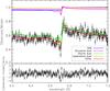 |
Fig. 10 Upper panel: a fit of the Si K-edge with particles of sizes in a range of 0.1−0.5 μm. The best-fitting mixture consists of the same compounds as the fit in Sect. 6.2: sample 1 (crystalline olivine) and sample 5 (amorphous pyroxene) with a small addition of sample 6 (hypersthene). Lower panel: model residuals of the fit in terms of the standard deviation, σ. |
8. Summary
In this paper, we analyze the X-ray spectrum of the low-mass X-ray binary GX 5-1, where we focuse, in particular, on the modeling of the Si K-edge. The Si K-edges of six silicate dust samples were measured at the Soleil synchrotron facility in Paris. Using these new measurements, we calculated the extinction profiles of these samples in order to make them suitable for the analysis of the ISM towards GX 5-1. The extinction profiles of the Si K-edge were added to the AMOL model of the spectral fitting program SPEX. We obtained a best fit to the Chandra HETG data of GX 5-1 and arrive at the following results:
-
1.
We established conservative lower limits on the abundances ofSi, O, Mg, and Fe: ASi/A⊙> 1.14, AO/A⊙> 1.06, AMg/A⊙> 1.6, AFe/A⊙> 0.79. Except for iron, all the lower limits on theabundances show abundances similar to, or above, protosolarvalues. We obtained upper limits on the depletion: <0.87 forsilicon, <0.23 for oxygen, <0.97 for magnesium and <0.76 for iron.
-
2.
There may be indications for large dust particles along the line of sight due to enhanced scattering features in the Si K-edge. The scattering feature longward of the Si K-edge is better fitted using a model with larger particles, which indicates the presence of particles larger than 0.25 μm up to 0.5 μm.
-
3.
The sharp absorption features observed in the Si K-edge suggest a possibly significant amount of crystalline dust with respect to the total amount of dust. However, more laboratory measurements are required to draw any conclusion on this subject.
See for an overview about C-statistics the SPEX manual: https://www.sron.nl/files/HEA/SPEX/manuals/manual.pdf and http://heasarc.gsfc.nasa.gov/lheasoft/xanadu/xspec/manual/XSappendixStatistics.html
Acknowledgments
Dust studies at SRON and Leiden Observatory are supported through the Spinoza Premie of the Dutch science agency, NWO. We would like to thank Jörn Wilms and the anonymous referee for providing us with helpful comments and suggestions. This research made use of the Chandra Transmission Grating Catalog and archive (http://tgcat.mit.edu). Furthermore, we made use of the FLUO correction code provided by Daniel Haskel. H.M. and S.Z. are grateful for support of the Deutsche Forschungsgemeinschaft under Mu 1164/7-2 and Mu 1164/8-1. We acknowledge SOLEIL for provision of synchrotron radiation facilities and we would like to thank Delphine Vantelon for assistance in using beamline LUCIA. E.C. acknowledges support from NWO-Vidi grant 639.042.525.
References
- Aitken, D. K., & Roche, P. F. 1984, MNRAS, 208, 751 [NASA ADS] [CrossRef] [Google Scholar]
- Anders, E., & Zinner, E. 1993, Meteoritics, 28, 490 [Google Scholar]
- Asai, K., Dotani, T., Nagase, F., & Mitsuda, K. 2000, ApJS, 131, 571 [NASA ADS] [CrossRef] [Google Scholar]
- Blommaert, J. A. D. L., de Vries, B. L., Waters, L. B. F. M., et al. 2014, A&A, 565, A109 [NASA ADS] [CrossRef] [EDP Sciences] [Google Scholar]
- Bohlin, R. C., Savage, B. D., & Drake, J. F. 1978, ApJ, 224, 132 [NASA ADS] [CrossRef] [Google Scholar]
- Bohren, C. F. 2010, Eur. J. Phys., 31, 573 [Google Scholar]
- Bradley, J. P. 1994, Science, 265, 925 [Google Scholar]
- Bringa, E. M., Kucheyev, S. O., Loeffler, M. J., et al. 2007, ApJ, 662, 372 [NASA ADS] [CrossRef] [Google Scholar]
- Bruzzoni, P., Carranza, R., Lacoste, J. C., & Crespo, E. 2002, Electrochimica Acta, 48, 341 [Google Scholar]
- Canizares, C. R., Davis, J. E., Dewey, D., et al. 2005, PASP, 117, 1144 [NASA ADS] [CrossRef] [Google Scholar]
- Cash, W. 1979, ApJ, 228, 939 [NASA ADS] [CrossRef] [Google Scholar]
- Chen, L., Hou, J. L., & Wang, J. J. 2003, AJ, 125, 1397 [NASA ADS] [CrossRef] [Google Scholar]
- Chiar, J. E., & Tielens, A. G. G. M. 2006, ApJ, 637, 774 [NASA ADS] [CrossRef] [Google Scholar]
- Christian, D. J., & Swank, J. H. 1997, ApJS, 109, 177 [NASA ADS] [CrossRef] [Google Scholar]
- Costantini, E., & de Vries, C. 2013, Mem. Soc. Astron. It., 84, 592 [NASA ADS] [Google Scholar]
- Costantini, E., Freyberg, M. J., & Predehl, P. 2005, A&A, 444, 187 [NASA ADS] [CrossRef] [EDP Sciences] [Google Scholar]
- Costantini, E., Pinto, C., Kaastra, J. S., et al. 2012, A&A, 539, A32 [NASA ADS] [CrossRef] [EDP Sciences] [Google Scholar]
- Dame, T. M., Hartmann, D., & Thaddeus, P. 2001, ApJ, 547, 792 [NASA ADS] [CrossRef] [Google Scholar]
- de Vries, C. P., & Costantini, E. 2009, A&A, 497, 393 [NASA ADS] [CrossRef] [EDP Sciences] [Google Scholar]
- de Vries, B. L., Min, M., Waters, L. B. F. M., Blommaert, J. A. D. L., & Kemper, F. 2010, A&A, 516, A86 [NASA ADS] [CrossRef] [EDP Sciences] [Google Scholar]
- Dorschner, J., Begemann, B., Henning, T., Jaeger, C., & Mutschke, H. 1995, A&A, 300, 503 [NASA ADS] [Google Scholar]
- Draine, B. T. 2003, ApJ, 598, 1026 [NASA ADS] [CrossRef] [Google Scholar]
- Draine, B. T. 2009, in Cosmic Dust – Near and Far, eds. T. Henning, E. Grün, & J. Steinacker, ASP Conf. Ser., 414, 453 [Google Scholar]
- Draine, B. T., & Lee, H. M. 1984, ApJ, 285, 89 [Google Scholar]
- Draine, B. T., & Li, A. 2001, ApJ, 551, 807 [NASA ADS] [CrossRef] [Google Scholar]
- Draine, B. T., & Li, A. 2007, ApJ, 657, 810 [NASA ADS] [CrossRef] [Google Scholar]
- Dwek, E., & Scalo, J. M. 1980, ApJ, 239, 193 [NASA ADS] [CrossRef] [Google Scholar]
- Dwek, E., Zubko, V., Arendt, R. G., & Smith, R. K. 2004, in Astrophysics of Dust, eds. A. N. Witt, G. C. Clayton, & B. T. Draine, ASP Conf. Ser., 309, 499 [Google Scholar]
- Flank, A.-M., Cauchon, G., Lagarde, P., et al. 2006, Nuclear Instruments and Methods in Physics Research Section B: Beam Interactions with Materials and Atoms, 246, 269 [Google Scholar]
- Floss, C., Stadermann, F. J., Bradley, J. P., et al. 2006, Geochim. Cosmochim. Acta, 70, 2371 [NASA ADS] [CrossRef] [Google Scholar]
- Gail, H.-P. 2010, in Lect. Notes Phys., 815, ed. T. Henning (Berlin: Springer Verlag), 61 [Google Scholar]
- Gail, H.-P., Zhukovska, S. V., Hoppe, P., & Trieloff, M. 2009, ApJ, 698, 1136 [NASA ADS] [CrossRef] [Google Scholar]
- Giacconi, R., Branduardi, G., Briel, U., et al. 1979, ApJ, 230, 540 [NASA ADS] [CrossRef] [Google Scholar]
- Henke, B., Gullikson, E., & Davis, J. 1993, Atomic Data and Nuclear Data Tables, 54, 181 [Google Scholar]
- Henning, T. 2010, ARA&A, 48, 21 [NASA ADS] [CrossRef] [Google Scholar]
- Henning, T., Begemann, B., Mutschke, H., & Dorschner, J. 1995, A&AS, 112, 143 [NASA ADS] [Google Scholar]
- Hoffman, J., & Draine, B. T. 2016, ApJ, 817, 139 [NASA ADS] [CrossRef] [Google Scholar]
- Jaeger, C., Molster, F. J., Dorschner, J., et al. 1998, A&A, 339, 904 [NASA ADS] [Google Scholar]
- Jenkins, E. B. 2009, ApJ, 700, 1299 [NASA ADS] [CrossRef] [Google Scholar]
- Jones, A. P., & Nuth, J. A. 2011, A&A, 530, A44 [NASA ADS] [CrossRef] [EDP Sciences] [Google Scholar]
- Jones, A. P., Tielens, A. G. G. M., Hollenbach, D. J., & McKee, C. F. 1994, ApJ, 433, 797 [NASA ADS] [CrossRef] [Google Scholar]
- Jones, A. P., Tielens, A. G. G. M., & Hollenbach, D. J. 1996, ApJ, 469, 740 [NASA ADS] [CrossRef] [Google Scholar]
- Jones, O. C., Kemper, F., Sargent, B. A., et al. 2012, MNRAS, 427, 3209 [NASA ADS] [CrossRef] [Google Scholar]
- Jura, M. 1980, ApJ, 235, 63 [NASA ADS] [CrossRef] [Google Scholar]
- Kaastra, J. S., Mewe, R., & Nieuwenhuijzen, H. 1996, in UV and X-ray Spectroscopy of Astrophysical and Laboratory Plasmas, eds. K. Yamashita, & T. Watanabe, 411 [Google Scholar]
- Kaastra, J. S., de Vries, C. P., Costantini, E., & den Herder, J. W. A. 2009, A&A, 497, 291 [NASA ADS] [CrossRef] [EDP Sciences] [Google Scholar]
- Keller, L. P., & Messenger, S. 2013, Geochim. Cosmochim. Acta, 107, 341 [NASA ADS] [CrossRef] [Google Scholar]
- Kemper, F., Markwick, A. J., & Woods, P. M. 2011, MNRAS, 413, 1192 [NASA ADS] [CrossRef] [Google Scholar]
- Kemper, F., Vriend, W. J., & Tielens, A. G. G. M. 2004, ApJ, 609, 826 [NASA ADS] [CrossRef] [Google Scholar]
- Kim, S.-H., & Martin, P. G. 1995, ApJ, 444, 293 [NASA ADS] [CrossRef] [Google Scholar]
- Lee, J. C., Ogle, P. M., Canizares, C. R., et al. 2001, ApJ, 554, L13 [NASA ADS] [CrossRef] [Google Scholar]
- Lee, J. C., Xiang, J., Ravel, B., Kortright, J., & Flanagan, K. 2009, ApJ, 702, 970 [NASA ADS] [CrossRef] [Google Scholar]
- Li, A., & Draine, B. T. 2001, ApJ, 550, L213 [NASA ADS] [CrossRef] [Google Scholar]
- Li, D., Bancroft, G. M., Fleet, M. E., & Feng, X. H. 1995, Phys. Chem. Miner., 22, 115 [NASA ADS] [Google Scholar]
- Lodders, K., & Palme, H. 2009, Meteoritics and Planetary Science Supplement, 72, 5154 [Google Scholar]
- Mathis, J. S. 1998, ApJ, 497, 824 [NASA ADS] [CrossRef] [Google Scholar]
- Mathis, J. S., Rumpl, W., & Nordsieck, K. H. 1977, ApJ, 217, 425 [NASA ADS] [CrossRef] [Google Scholar]
- Meikle, W. P. S., Mattila, S., Pastorello, A., et al. 2007, ApJ, 665, 608 [NASA ADS] [CrossRef] [Google Scholar]
- Meitner, L. 1922, Zeitschrift fur Physik, 9, 131 [Google Scholar]
- Messenger, S., Keller, L. P., & Lauretta, D. S. 2005, Science, 309, 737 [NASA ADS] [CrossRef] [PubMed] [Google Scholar]
- Meurant, G. 1983, Solid State Physics, Solid State Physics No. v. 37 (Elsevier Science) [Google Scholar]
- Mie, G. 1908, Ann. Phys., 330, 377 [Google Scholar]
- Min, M., Dominik, C., Hovenier, J. W., de Koter, A., & Waters, L. B. F. M. 2006, A&A, 445, 1005 [NASA ADS] [CrossRef] [EDP Sciences] [MathSciNet] [Google Scholar]
- Min, M., Waters, L. B. F. M., de Koter, A., et al. 2007, A&A, 462, 667 [NASA ADS] [CrossRef] [EDP Sciences] [Google Scholar]
- Min, M., Hovenier, J. W., Waters, L. B. F. M., & de Koter, A. 2008, A&A, 489, 135 [NASA ADS] [CrossRef] [EDP Sciences] [Google Scholar]
- Molster, F. J., Waters, L. B. F. M., & Tielens, A. G. G. M. 2002a, A&A, 382, 222 [NASA ADS] [CrossRef] [EDP Sciences] [Google Scholar]
- Molster, F. J., Waters, L. B. F. M., Tielens, A. G. G. M., & Barlow, M. J. 2002b, A&A, 382, 184 [NASA ADS] [CrossRef] [EDP Sciences] [Google Scholar]
- Molster, F. J., Waters, L. B. F. M., Tielens, A. G. G. M., Koike, C., & Chihara, H. 2002c, A&A, 382, 241 [NASA ADS] [CrossRef] [EDP Sciences] [Google Scholar]
- Mutschke, H., Min, M., & Tamanai, A. 2009, A&A, 504, 875 [NASA ADS] [CrossRef] [EDP Sciences] [Google Scholar]
- Nittler, L. R. 2005, ApJ, 618, 281 [NASA ADS] [CrossRef] [Google Scholar]
- Nittler, L., Alexander, C., Gao, X., Walker, R., & Zinner, E. 1997, Nucl. Phys. A, 621, 113 [NASA ADS] [CrossRef] [Google Scholar]
- Olofsson, J., Augereau, J.-C., van Dishoeck, E. F., et al. 2009, A&A, 507, 327 [NASA ADS] [CrossRef] [EDP Sciences] [Google Scholar]
- Olofsson, J., Juhász, A., Henning, T., et al. 2012, A&A, 542, A90 [NASA ADS] [CrossRef] [EDP Sciences] [Google Scholar]
- Ormel, C. W., Paszun, D., Dominik, C., & Tielens, A. G. G. M. 2009, A&A, 502, 845 [NASA ADS] [CrossRef] [EDP Sciences] [Google Scholar]
- Ormel, C. W., Min, M., Tielens, A. G. G. M., Dominik, C., & Paszun, D. 2011, A&A, 532, A43 [NASA ADS] [CrossRef] [EDP Sciences] [Google Scholar]
- Ossenkopf, V., Henning, T., & Mathis, J. S. 1992, A&A, 261, 567 [NASA ADS] [Google Scholar]
- Pinto, C., Kaastra, J. S., Costantini, E., & Verbunt, F. 2010, A&A, 521, A79 [NASA ADS] [CrossRef] [EDP Sciences] [Google Scholar]
- Pinto, C., Kaastra, J. S., Costantini, E., & de Vries, C. 2013, A&A, 551, A25 [NASA ADS] [CrossRef] [EDP Sciences] [Google Scholar]
- Poe, B., Seifert, F., Sharp, T., & Wu, Z. 1997, Physics and Chemistry of Minerals, 24, 477 [Google Scholar]
- Posch, T., Kerschbaum, F., Mutschke, H., Dorschner, J., & Jäger, C. 2002, A&A, 393, L7 [NASA ADS] [CrossRef] [EDP Sciences] [Google Scholar]
- Predehl, P., & Schmitt, J. H. M. M. 1995, A&A, 293, 889 [NASA ADS] [Google Scholar]
- Rho, J., Kozasa, T., Reach, W. T., et al. 2008, ApJ, 673, 271 [NASA ADS] [CrossRef] [Google Scholar]
- Rho, J., Reach, W. T., Tappe, A., et al. 2009, ApJ, 700, 579 [NASA ADS] [CrossRef] [Google Scholar]
- Roche, P. F., & Aitken, D. K. 1984, MNRAS, 208, 481 [NASA ADS] [Google Scholar]
- Roche, P. F., & Aitken, D. K. 1985, MNRAS, 215, 425 [NASA ADS] [CrossRef] [Google Scholar]
- Savage, B. D., & Sembach, K. R. 1996, ARA&A, 34, 279 [NASA ADS] [CrossRef] [Google Scholar]
- Smith, R. K., Dame, T. M., Costantini, E., & Predehl, P. 2006, ApJ, 648, 452 [NASA ADS] [CrossRef] [Google Scholar]
- Spoon, H. W. W., Tielens, A. G. G. M., Armus, L., et al. 2006, ApJ, 638, 759 [NASA ADS] [CrossRef] [Google Scholar]
- Stern, E., Newville, M., Ravel, B., Yacoby, Y., & Haskel, D. 1995, Physica B: Condensed Matter, 208, 117 [Google Scholar]
- Tielens, A. G. G. M. 2008, ARA&A, 46, 289 [NASA ADS] [CrossRef] [EDP Sciences] [Google Scholar]
- Tielens, A. G. G. M., Wooden, D. H., Allamandola, L. J., Bregman, J., & Witteborn, F. C. 1996, ApJ, 461, 210 [NASA ADS] [CrossRef] [PubMed] [Google Scholar]
- Trümper, J. 1982, Adv. Space Res., 2, 241 [NASA ADS] [CrossRef] [Google Scholar]
- Ueda, Y., Mitsuda, K., Murakami, H., & Matsushita, K. 2005, ApJ, 620, 274 [NASA ADS] [CrossRef] [Google Scholar]
- Valencic, L. A., & Smith, R. K. 2013, ApJ, 770, 22 [NASA ADS] [CrossRef] [Google Scholar]
- Van de Hulst, H. C. 1958, ZAp, 45, 149 [NASA ADS] [Google Scholar]
- Voshchinnikov, N. V., Il’in, V. B., Henning, T., & Dubkova, D. N. 2006, A&A, 445, 167 [NASA ADS] [CrossRef] [EDP Sciences] [Google Scholar]
- Weingartner, J. C., & Draine, B. T. 2001, ApJ, 548, 296 [NASA ADS] [CrossRef] [Google Scholar]
- Westphal, A. J., Stroud, R. M., Bechtel, H. A., et al. 2014, Science, 345, 786 [NASA ADS] [CrossRef] [Google Scholar]
- Whittet, D. C. B., 2003, Dust in the galactic environment (Bristol: Institute of Physics, IOP) [Google Scholar]
- Whittet, D. C. B., Boogert, A. C. A., Gerakines, P. A., et al. 1997, ApJ, 490, 729 [NASA ADS] [CrossRef] [Google Scholar]
- Wilms, J., Allen, A., & McCray, R. 2000, ApJ, 542, 914 [NASA ADS] [CrossRef] [Google Scholar]
- Wiscombe, W. J. 1980, Appl. Opt., 19, 1505 [NASA ADS] [CrossRef] [PubMed] [Google Scholar]
- Wooden, D. H., Rank, D. M., Bregman, J. D., et al. 1993, ApJS, 88, 477 [NASA ADS] [CrossRef] [Google Scholar]
- Wooden, D. H., Harker, D. E., Woodward, C. E., et al. 1999, ApJ, 517, 1034 [NASA ADS] [CrossRef] [Google Scholar]
- Xue, M., Jiang, B. W., Gao, J., et al. 2016, ApJS, 224, 23 [NASA ADS] [CrossRef] [Google Scholar]
- Yao, Y., & Wang, Q. D. 2005, ApJ, 624, 751 [NASA ADS] [CrossRef] [Google Scholar]
- Yao, Y., Schulz, N., Wang, Q. D., & Nowak, M. 2006, ApJ, 653, L121 [NASA ADS] [CrossRef] [Google Scholar]
- Zubko, V., Dwek, E., & Arendt, R. G. 2004, ApJS, 152, 211 [NASA ADS] [CrossRef] [Google Scholar]
Appendix A: Correction for saturation
In Sect. 3, we describe the effect of saturation. In order to correct for saturation, we used the FLUO correction code by Daniel Haskel, which is part of the UWXAFS software package (Stern et al. 1995). In this appendix, we give a brief summary of the correction method, which can also be found in the documentation of the FLUO code. Equation (3) corresponds to pre-edge subtracted data, that is, for energies lower than the edge If/I0, which is zero. The signal can be normalized by performing an edge-step normalization. The normalized signal N is given by: ![Mathematical equation: \appendix \setcounter{section}{1} \begin{equation} N= \dfrac{\frac{I_{\rm f}}{I_0}(E)}{\frac{I_{\rm f}}{I_0}(E_0^{+})}=\Bigg[\dfrac{\epsilon_{\rm f}(E)\alpha_e(E)}{\epsilon_{\rm f}(E_0^{+})\alpha_e(E_0^+)}\Bigg]\Bigg[\dfrac{\alpha_{\mathrm{tot}}(E_{\rm f})+\alpha_{\rm b}(E_0^+)+\alpha_e(E_0^+)}{\alpha_\mathrm{tot}(E_{\rm f})+\alpha_{\rm b}(E)+\alpha_e(E)}\Bigg], \end{equation}](/articles/aa/full_html/2017/03/aa28507-16/aa28507-16-eq197.png) (A.1)where αtot = αb + αe, αe is the absorption from the element of interest, αb denotes the absorption from all other atoms and other edges of interest and
(A.1)where αtot = αb + αe, αe is the absorption from the element of interest, αb denotes the absorption from all other atoms and other edges of interest and  indicates the energy above the main absorption edge. Dividing the denominator by
  gives:
 ![Mathematical equation: \appendix \setcounter{section}{1} \begin{equation} N = \dfrac{\alpha_e(E)}{\alpha_e(E_0^{+})}\dfrac{\epsilon_{\rm f}(E)}{\epsilon_{\rm f}(E_0^{+})} \left[\dfrac{\frac{\alpha_{\mathrm{tot}}(E_{\rm f})}{\alpha_e(E_0^{+})}+\frac{\alpha_{\rm b}(E_0^{+})}{\alpha_e(E_0^{+})}+\frac{\alpha_e(E_0^+)}{\alpha_e(E_0^+)}}{\frac{\alpha_{\mathrm{tot}}(E_{\rm f})}{\alpha_e(E_0^+)}+\frac{\alpha_{\rm b}(E)}{\alpha_e(E_0^+)}+\frac{\alpha_e(E)}{\alpha_e(E_0^{+})}}\right]\cdot \end{equation}](/articles/aa/full_html/2017/03/aa28507-16/aa28507-16-eq203.png) (A.2)Defining
(A.2)Defining  ,
,  , and
, and  and solving for
  gives:
  (A.3)Since we are only concerned with a small energy range at the interval of the XANES region, the following approximation was made:
  in Eq. (A.3). Furthermore,
  which leads to: γ ≈ γ′. FLUO uses tabulated cross-section from the McMaster tables to calculate β and γ. It will also perform an edge-step normalization in order to obtain N. In this way
  can be derived.
Appendix B: Si K-edge models
Here we show the extinction profiles around the Si K-edge for the compounds used in this analysis. These profiles are implemented in the AMOL model of the fitting code SPEX. The numbers of the samples correspond to the numbers given in Table 1 in which the chemical formulas and the structure (crystalline or amorphous) are given. The absolute cross-sections of the models used in this analysis are available in tabular form6.
 |
Fig. B.1 Transmission of the six dust extinction models (absorption and scattering) from the analysis of the Si K-edge. The silicon column density has been set here to 1018 cm-2 for all the dust models. Each model is indicated by a number corresponding to the numbers in Table 1. The table also gives the chemical formula and the structure (crystalline or amorphous) of the dust compound. |
All Tables
All Figures
|
Fig. 1 Example of the difference between the sample corrected for saturation and the uncorrected measurement. Shown is sample 3, crystalline pyroxene. The lower panel shows the ratio of the corrected and uncorrected measurement. |
| In the text | |
|
Fig. 2 Si K-edge of the six samples. The x-axis shows the energy in Å and the y-axis shows the amount of absorption indicated by the cross-section (in Mb per Si atom). |
| In the text | |
|
Fig. 3 Refractive index of sample 1 (olivine). The upper panel shows the real part of the refractive index (n) and the lower panel shows the imaginary part of the refractive index (k). |
| In the text | |
|
Fig. 4 Model of the Si K-edge of olivine (sample 1) as implemented in SPEX, without the continuum of the extinction profile. The cross-section in Mb is given per Si-atom. |
| In the text | |
|
Fig. 5 Continuum of GX 5-1. Data from the HEG short exposure, MEG short exposure, and HEG long exposure (OBSID 716) were used to fit the continuum. The resulting fit to each of the three data sets is shown by a red line. The model consists of two absorbed black bodies. The two black bodies in the model are represented in the figure by the green and blue lines. For clarity, only the black body models of the HEG grating (both long and short exposure) are shown and the MEG data has been omitted in the figure, therefore each black body model shows two curves. |
| In the text | |
|
Fig. 6 Fit to the spectrum of GX 5-1 is shown in red. The contribution of the continuum is divided out. The other lines show the contribution of the absorbing components to the transmission. The purple line shows the contribution of pyroxene (sample 5), the green line the contribution of olivine (sample 1), and the blue line the contribution of gas. The lower panel shows the model residuals of the fit in terms of the standard deviation, σ. |
| In the text | |
|
Fig. 7 Upper panel: a fit of the Si K-edge, where the depletion of silicon is left as a free parameter without boundary values. The best fitting mixture consist of the same compounds as the fit in Sect. 6.2: sample 1 (crystalline olivine) and sample 5 (amorphous pyroxene). Lower panel: model residuals of the fit in terms of the standard deviation, σ. |
| In the text | |
|
Fig. 8 Comparison of the best fit (upper left window) with iron-poor dust mixtures, strictly crystalline mixtures, and amorphous mixtures. |
| In the text | |
|
Fig. 9 Effect of a change in the size distribution on the extinction. The olivine Si K-edge with a MRN distribution with particle sizes of 0.005−0.25 μm microns is shown in red. The blue line shows the same edge, but now the particle sizes range between 0.05 and 0.5 μm. |
| In the text | |
|
Fig. 10 Upper panel: a fit of the Si K-edge with particles of sizes in a range of 0.1−0.5 μm. The best-fitting mixture consists of the same compounds as the fit in Sect. 6.2: sample 1 (crystalline olivine) and sample 5 (amorphous pyroxene) with a small addition of sample 6 (hypersthene). Lower panel: model residuals of the fit in terms of the standard deviation, σ. |
| In the text | |
|
Fig. B.1 Transmission of the six dust extinction models (absorption and scattering) from the analysis of the Si K-edge. The silicon column density has been set here to 1018 cm-2 for all the dust models. Each model is indicated by a number corresponding to the numbers in Table 1. The table also gives the chemical formula and the structure (crystalline or amorphous) of the dust compound. |
| In the text | |
Current usage metrics show cumulative count of Article Views (full-text article views including HTML views, PDF and ePub downloads, according to the available data) and Abstracts Views on Vision4Press platform.
Data correspond to usage on the plateform after 2015. The current usage metrics is available 48-96 hours after online publication and is updated daily on week days.
Initial download of the metrics may take a while.