| Issue |
A&A
Volume 597, January 2017
|
|
|---|---|---|
| Article Number | A29 | |
| Number of page(s) | 17 | |
| Section | Stellar structure and evolution | |
| DOI | https://doi.org/10.1051/0004-6361/201629126 | |
| Published online | 19 December 2016 | |
Asteroseismology of hybrid δ Scuti-γ Doradus pulsating stars
1 Facultad de Ciencias Astronómicas y Geofísicas, Universidad Nacional de La Plata, Paseo del Bosque s/n, 1900 La Plata, 19000 La plata, Argentina
2 Instituto de Astrofísica La Plata, CONICET-UNLP, Argentina
e-mail: This email address is being protected from spambots. You need JavaScript enabled to view it.
; This email address is being protected from spambots. You need JavaScript enabled to view it.
; This email address is being protected from spambots. You need JavaScript enabled to view it.
Received: 16 June 2016
Accepted: 7 September 2016
Abstract
Context. Hybrid δ Scuti-γ Doradus pulsating stars show acoustic (p) oscillation modes typical of δ Scuti variable stars, and gravity (g) pulsation modes characteristic of γ Doradus variable stars simultaneously excited. Observations from space missions such as MOST, CoRoT, and Kepler have revealed a large number of hybrid δ Scuti-γ Doradus pulsators, thus paving the way for an exciting new channel of asteroseismic studies.
Aims. We perform detailed asteroseismological modelling of five hybrid δ Scuti-γ Doradus stars.
Methods. A grid-based modeling approach was employed to sound the internal structure of the target stars using stellar models ranging from the zero-age main sequence to the terminal-age main sequence, varying parameters such as stellar mass, effective temperature, metallicity and core overshooting. Their adiabatic radial (ℓ = 0) and non-radial (ℓ = 1,2,3) p and g mode periods were computed. Two model-fitting procedures were used to search for asteroseismological models that best reproduce the observed pulsation spectra of each target star.
Results. We derive the fundamental parameters and the evolutionary status of five hybrid δ Scuti-γ Doradus variable stars recently observed by the CoRoT and Kepler space missions: CoRoT 105733033, CoRoT 100866999, KIC 11145123, KIC 9244992, and HD 49434. The asteroseismological model for each star results from different criteria of model selection, in which we take full advantage of the richness of periods that characterises the pulsation spectra for this kind of star.
Key words: asteroseismology / stars: interiors / stars: oscillations / stars: variables: δ Scuti / stars: variables: γ Doradus
© ESO, 2016
1. Introduction
At the present time, pulsating stars constitute one of the most powerful tools for sounding stellar interiors and also provide a wealth of information about the physical structure and evolutionary status of stars through asteroseismology (Aerts et al. 2010; Balona 2010; Catelan & Smith 2015). Nowadays, a huge number of variable stars are routinely discovered and scrutinised by space missions such as MOST (Walker et al. 2003), CoRoT (Baglin et al. 2009) and Kepler (Koch et al. 2010), which include long-term monitoring with high-temporal resolution and high-photometric sensibility for hundreds of thousands of stars. Among the most intensively studied classes of variable stars in recent years we found the δ Scuti (Sct) and γ Doradus (Dor), which contain ~1.2−2.2 M⊙ stars with spectral types between A and F, undergoing quiescent core H burning at (or near to) the main sequence (MS) (6500 K ≲ Teff ≲ 8500 K). They exhibit multiperiodic brightness variations due to global radial and non-radial pulsation modes.
The δ Sct stars, discovered over a century ago (Campbell & Wright Campbell & Wright 1900), display high-frequency variations with typical periods in the range of ~0.008−0.42 d, and amplitudes from milli-magnitudes up to almost one magnitude in blue bands. They are likely produced by non-radial p modes of low radial order n and low harmonic degree (ℓ = 1−3), although the largest amplitude variations are probably induced by the radial fundamental mode (n = 0,ℓ = 0) and/or low-overtone radial modes (n = 1,2,3,...,ℓ = 0). The fact that δ Sct stars pulsate in non-radial p modes and radial modes implies that they are potentially useful for probing the stellar envelope. The δ Sct variables are Population I stars of spectral type between A0 and F5, lying on the extension of the Cepheid instability strip towards low luminosities and at effective temperatures between 7000 K and 8500 K, with stellar masses in the interval between 1.5 and 2.2 M⊙, and luminosities in the range 5 ≲ L/L⊙ ≲ 80 (Catelan & Smith 2015). The projected rotation velocities are in the range [0,150] km s-1, although they can reach values up to ~250 km s-1. The pulsations are thought to be driven by the κ mechanism (Cox 1980; Unno et al. 1989) operating in the partial ionization zone of He II (Chevalier 1971; Dupret et al. 2004; Grigahcène et al. 2005). Stochastically driven solar-like oscillations have also been predicted to occur in δ Sct stars (Samadi et al. 2002). Notably, these expectations have been confirmed for one object (Antoci et al. 2011). Among δ Sct stars, a distinction is frequently made between the so called high-amplitude δ Sct stars (HADS), whose amplitudes in the V band exceed 0.3 mag, and their much more abundant low-amplitude δ Sct star (LADS) counterparts (see Lee et al. 2008). There exists a Population II counterpart to δ Sct variables, the so called SX Phoenicis (Phe), which are usually observed in low-metallicity globular clusters (see, e.g. Arellano Ferro et al. 2014).
The γ Dor variables (Kaye et al. 1999), were recognized as a new class of pulsating stars approximately 20 years ago (Balona et al. 1994). They are generally cooler than δ Sct stars, with Teff between 6700 K and 7400 K (spectral types between A7 and F5) and masses in the range 1.5 to 1.8 M⊙ (Catelan & Smith 2015). The γ Dor stars pulsate in low-degree, high-order g modes driven by a flux modulation mechanism called convective blocking and induced by the outer convective zone (Guzik et al. 2000; Dupret et al. 2004; Grigahcène et al. 2005). The low-frequency variations shown by these stars have periods typically between ~0.3 d and ~3 d and amplitudes below ~0.1 mag. The presence of g modes in γ Dor stars offers an opportunity to probe into the core regions. In addition, since high-order g modes are excited (n ≫ 1), it is possible to use the asymptotic theory (Tassoul 1980) and the departures from uniform period spacing (by mode trapping) to explore the possible chemical inhomogeneities in the structure of the convective cores (Miglio et al. 2008). Stochastic excitation of solar like oscillations has also been predicted in γ Dor stars (Pereira et al. 2007), but no positive detection has yet been reported.
The instability strips of δ Sct and γ Dor stars partially overlap in the Hertzprung-Russell (HR) diagram (see, for instance, Fig. 4 of Tkachenko et al. 2013), strongly suggesting the existence of δ Sct-γ Dor hybrid stars, that is, stars simultaneously showing high-frequency p-mode pulsations typical of δ Sct stars and low-frequency g-mode oscillations characteristic of γ Dor stars (Dupret et al. 2004; Grigahcène et al. 2010). The first example of a star pulsating intrinsically with both δ Sct and γ Dor frequencies was detected from the ground (Henry & Fekel 2005). Other examples are HD 49434 (Uytterhoeven et al. 2008) and HD 8801 (Handler 2009). A large sample of Kepler and CoRoT stars yielded the first hint that hybrid behavior might be common in A-F type stars (Grigahcène et al. 2010; Hareter et al. 2010). A follow up study with a large sample (>750 stars) of δ Sct and γ Dor candidates by Uytterhoeven et al. (2011) revealed that out of 471 stars showing δ Sct or γ Dor pulsations, 36% (171 stars) are hybrid δ Sct-γ Dor stars. Very recent studies (e.g. Bradley et al. 2015) analysing larger samples of δ Sct or γ Dor candidates strongly suggest that hybrid δ Sct-γ Dor stars are very common. Balona et al. (2015) studied the frequency distributions of δ Sct stars observed by the Kepler telescope in short-cadence mode and found low frequencies (typical of γ Dor stars) in all the analyzed δ Sct stars. This finding renders somewhat meaningless the concept of δ Sct-γ Dor hybrids.
Apart from these important investigations of large samples of stars, there are published studies on several individual hybrid δ Sct-γ Dor stars observed from space missions. Among them, we mention HD 114839 (King et al. 2006) and BD+18-4914 (Rowe et al. 2006), both detected by the MOST satellite. Furthermore, hybrid δ Sct-γ Dor stars discovered with CoRoT observations are CoRoT 102699796 (Ripepi et al. 2011), CoRoT 105733033 (Chapellier et al. 2012), CoRoT 100866999 (Chapellier & Mathias 2013), and HD 49434 Brunsden et al. (2015). Finally, among hybrid stars discovered with the Kepler mission, we mention KIC 6761539 (Herzberg et al. 2012), KIC 11145123 (Kurtz et al. 2014), KIC 8569819 (Kurtz et al. 2015), KIC 9244992 (Saio et al. 2015), KIC 9533489 (Bognár et al. 2015) and KIC 10080943 (Keen et al. 2015).
Several attempts at asteroseismic modelling of δ Sct stars have shown it to be a very difficult task (Civelek et al. 2001, 2003; Lenz et al. 2008; Murphy et al. 2013). In part, this is due to there generally being many combinations of the stellar structure parameters (Teff,M⋆,Y,Z, overshooting, etc.) that lead to very different seismic solutions but reproduce, with virtually the same degree of precision, the set of observed frequencies. The situation is potentially much more favourable in the case of hybrid δ Sct-γ Dor stars because the simultaneous presence of both g and p non-radial excited modes (in addition to radial pulsations) allows one to place strong constraints on the whole structure, thus eliminating most of the degeneration of solutions. As such, hybrid stars have a formidable asteroseismological potential and are very attractive targets for modelling.
Among the above mentioned hybrid objects, detailed seismological modelling has so far been performed for only a few δ Sct-γ Dor hybrids; namely KIC 11145123 (Kurtz et al. 2014), KIC 9244992 (Saio et al. 2015) and the binary system KIC 10080943 (Schmid & Aerts 2016). In this study, we present a seismic model of five δ Sct-γ Dor hybrids including those two studied by Kurtz et al. (2014) and Saio et al. (2015). Our approach consists of the comparison of the observed pulsation periods with the theoretical adiabatic pulsation periods (and period spacings in the case of high-order g modes) computed on a huge set of stellar models representative of A-F MS stars with masses in the range 1.2−2.2 M⊙ generated with a state-of-the-art evolutionary code. This approach is frequently referred to as grid-based or forward modelling in the field of solar-like oscillations (e.g. Gai et al. 2011; Hekker & Ball 2014) and has been the preferred asteroseismological approach for pulsating white dwarfs (Córsico et al. 2008; Althaus et al. 2010; Romero et al. 2012). Furthermore, this approach has been adopted for the study of δ Sct-γ Dor hybrid stars by Schmid & Aerts (2016). Also, a similar approach has been adopted by Moravveji et al. (2015, 2016) in the context of slowly pulsating B (SPB) stars. The characteristics of the target stars are determined by searching among the grid of models to get a “best-fit” model for a given observed set of periods of radial modes, and p and g non-radial modes. In particular, we make full use of the valuable property that some hybrid stars offer, that is, the value of the mean period spacing  of g modes. Specifically, we perform asteroseismic modelling of the hybrid δ Sct-γ Dor stars CoRoT 105733033 (Chapellier et al. 2012), CoRoT 100866999 (Chapellier & Mathias 2013), KIC 11145123 (Kurtz et al. 2014), KIC 9244992 (Saio et al. 2015) and HD 49434 Brunsden et al. (Brunsden et al. 2015). The use of
  allows us to discard a large portion of the grid of models; those that do not reproduce the observed period spacing. Also we assume, as usual, that the largest amplitude mode in the δ Sct region of the pulsation spectrum is associated with the fundamental radial mode (ℓ = 0,n = 0) or the first radial overtone modes (ℓ = 0,n = 1,2,3,4,...). This step further reduces the number of possible seismological models. Finally, we perform a period-to-period fit to the p mode periods. We also carry out other possible model selections, for instance, by performing direct period-to-period fits to the complete set of observed periods (including individual periods of g modes and radial modes). This research constitutes the first stage of an ongoing systematic asteroseismic modeling program of hybrid δ Sct-γ Dor stars at the La Plata Observatory.
This article is organized as follows: in Sect. 2 we describe our evolutionary and pulsation numerical tools. The main ingredients of the model grid we use to assess the pulsation properties of hybrid δ Sct-γ Dor stars are described in Sect. 3. Section 4 is devoted to describing the effects that core overshooting and metallicity have on the pulsation properties of g and p modes. In Sect. 5 we present in detail our asteroseismic analysis of the target stars. Finally, in Sect. 6 we summarise our main findings.
2. Numerical tools
2.1. Stellar evolution code
We carried out an asteroseismological analysis of δ Sct-γ Dor stars by computing a huge grid of evolutionary and pulsational models representative of this kind of variable star. The complete grid of models and some of their relevant pulsation properties will be described in detail in Sect. 3. The stellar models were generated with the help of the LPCODE (Althaus et al. 2005) stellar evolution code which has been developed entirely at La Plata Observatory. LPCODE is a well-tested and widely-employed stellar code which is able to simulate the evolution of low- and intermediate-mass stars from the zero-age main sequence (ZAMS), through the core H-burning phase, the He-burning phase, and the thermally pulsing asymptotic giant branch (AGB) phase to the white dwarf (WD) stage. The code has been used in a variety of studies involving the formation and evolution of WDs (Renedo et al. 2010; Althaus et al. 2012; Salaris et al. 2013), extremely low-mass (ELM) WD stars (Althaus et al. 2013), H-deficient PG1159 stars resulting from very late thermal pulses (VLTP) and the “born-again scenario” (Althaus et al. 2005; Miller Bertolami & Althaus 2006), sdB and sdO stars (Miller Bertolami et al. 2008, 2012), and low-mass giant stars considering fingering convection (Wachlin et al. 2011, 2014).
LPCODE is based on the Kippenhahn (1967) method for calculating stellar evolution. The code has the capability to generate stellar models with an arbitrary number of mesh points by means of an algorithm that adds mesh points where they are necessary (where physical variables change appreciably) and eliminates them where they are not. The main physical ingredients of LPCODE, relevant to our analysis of hybrid δ Sct-γ Dor, include: radiative opacities of OPAL project Iglesias & Rogers (1996) complemented at low temperatures with the molecular opacities produced by Ferguson et al. (2005); equation of state (EoS) at low-density regime of OPAL project, comprising the partial ionization for H and He compositions, the radiation pressure and the ionic contribution; and the nuclear network, which considers the following 16 elements: 1H, 2H, 3He, 4He, 7Li, 7Be, 12C, 13C, 14N, 15N, 16O, 17O, 18O, 19Fe, 20Ne, 22Ne and 34 thermonuclear reaction rates to describe the H (proton-proton chain and CNO bi-cycle) and He burning and C ignition. The abundance changes for all chemical elements are described thus: ![Mathematical equation: \begin{equation} \left(\frac{{\rm d}Y}{{\rm d}t}\right)= \left(\frac{\partial Y}{\partial t}\right)_{\rm nuc} + \frac{\partial}{\partial M_r}\left[(4\pi r^2 \rho)^2 D\frac{\partial Y}{\partial M_r}\right], \label{difusion} \end{equation}](/articles/aa/full_html/2017/01/aa29126-16/aa29126-16-eq50.png) (1)
(1)
Y being the vector containing fractions of all the considered nuclear species. The first term of Eq. (1) gives the abundance changes due to thermonuclear reactions. Details about the numerical procedure for solving these equations can be found in Althaus et al. (2003). All of our models have a convective core since we considered masses in the range 1.2−2.2 M⊙. For some of them we consider the occurrence of core overshooting, that is, mixing of chemical elements beyond the formal convective boundary set by the Schwarzschild criterion ∇ad< ∇rad (∇ad and ∇rad being the adiabatic and radiative temperature gradients; see Kippenhahn et al. 2012). Semiconvection, that is, the mixing of layers for which ∇ad< ∇rad< ∇L (where ∇L is the Ledoux temperature gradient; see Kippenhahn et al. 2012, for its definition) is not taken into account. We note that semiconvective layers on top of the convective zone may vary the extent of the convective core. In LPCODE, mixing due to convection, salt finger and overshoot are treated as diffusion processes (second term of Eq. (1)). The salt finger instability takes place when the stabilising agent (heat) diffuses away faster than the destabilising agent (μ), leading to a slow mixing process that might provide extra mixing (Charbonnel & Zahn 2007). The efficiency of convective and salt-finger mixing is described by appropriate diffusion coefficients D which are specified by our treatment of convection. Here, we adopted the classical mixing length theory (MLT) for convection (see, e.g. Kippenhahn et al. 2012) with the free parameter α = 1.66, with which we reproduce the present luminosity and effective temperature of the Sun, L⊙ = 3.842 × 1033 erg s-1 and log Teff = 3.7641, when Z = 0.0164 and X = 0.714 are adopted, according to the Z/X value of Grevesse & Noels (1993). Extra-mixing episodes (overshooting) are taken into account as time dependent diffusion processes, assuming that the mixing velocities decay exponentially beyond convective boundaries with a diffusion coefficient given by: 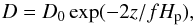 (2)
(2)
where D0 is the diffusive coefficient near the edge of the convective zone, z is the geometric distance of the considered layer to this edge, HP is the pressure scale height at the convective boundary and f is a measure of the extent of the overshoot region (Herwig et al. 1997; Herwig 2000). In this study we consider several values for f (see Sect. 3).
2.2. Pulsation code
The pulsation computations employed in this work were carried out with the adiabatic version of the LP-PUL pulsation code described in detail in Córsico & Althaus (2006), which is coupled to the LPCODE evolutionary code. Briefly, the LP-PUL pulsation code is based on the general Newton-Raphson technique to solve the full set of equations and boundary conditions that describe linear, adiabatic, radial and non-radial stellar pulsations following the dimensionless formulation of Dziembowski (1971). The pulsation code provides the dimensionless eigenfrequency ωn (n being the radial order of the mode) and eigenfunctions y1,...,y4. From these basic quantities, the code computes the pulsation periods (Πn), the oscillation kinetic energy (Kn), the first order rotation splitting coefficients (Cn), the weight functions (wn), and the variational periods ( ) for each computed eigenmode. Generally, the relative difference between and Πn is lower than ~10-4 (that is, ~0.01 %). This represents the precision with which LP-PUL code computes the pulsation periods (see Córsico & Benvenuto 2002, for details). The set of pulsation equations, boundary conditions, and pulsation quantities of relevance to this work are given in the appendix section of Córsico & Althaus (2006). The LP-PUL pulsation code has been tested and extensively used in numerous asteroseismological studies of pulsating WDs and pre-WDs (Córsico et al. 2001, 2005; Córsico & Althaus 2006; Córsico et al. 2008, 2012; Córsico & Althaus 2014b,a; Romero et al. 2012, 2013), as well as hot subdwarf stars sdB and sdO (Miller Bertolami et al. 2011, 2012). Recently, it has been employed for the first time to explore the pulsation properties of δ Sct and γ Dor stars (Sánchez Arias et al. 2013).
For g modes with high radial order n (long periods), the separation of consecutive periods (| Δn | = 1) becomes nearly constant at a value dependent on ℓ, given by the asymptotic theory of non-radial stellar pulsations. In LP-PUL, the asymptotic period spacing for g modes is computed as in Tassoul (1990): ![Mathematical equation: \begin{equation} \Delta \Pi^{a}_{\ell}= \frac{2\pi^2}{\sqrt{\ell(\ell+1)}} \left[\int_{r_1}^{r_2}\frac{N}{r}{\rm d}r\right]^{-1} \label{aps} , \end{equation}](/articles/aa/full_html/2017/01/aa29126-16/aa29126-16-eq80.png) (3)
(3)
where r1 and r2 are the radius of the inner and outer boundaries of the propagation region, respectively. For p modes with high radial order (high frequencies), the separation of consecutive frequencies becomes nearly constant and independent from ℓ, at a value given by Unno et al. (1989) and the following equation: ![Mathematical equation: \begin{equation} \Delta \nu^{\rm a} = \left[ 2 \int_0^R \frac{{\rm d}r}{c_{\rm s}}\right]^{-1}, \label{afs} \end{equation}](/articles/aa/full_html/2017/01/aa29126-16/aa29126-16-eq83.png) (4)
(4)
where cs is the local adiabatic sound speed, defined as  .
.
In our code, the squared Lamb frequency (Lℓ, one of the critical frequencies of non-radial stellar pulsations) is computed as: 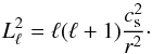 (5)On the other hand, the squared Brunt-Väisälä frequency (N, the other critical frequency of non-radial stellar pulsations) is computed as (Tassoul 1990):
 ![Mathematical equation: \begin{equation} \label{bv} N^2= \frac{g^2 \rho}{P}\frac{\chi_{\rm T}}{\chi_{\rho}} \left[\nabla_{\rm ad}- \nabla + B\right], \end{equation}](/articles/aa/full_html/2017/01/aa29126-16/aa29126-16-eq89.png) (6)where the compressibilities are defined as
(6)where the compressibilities are defined as 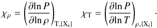 (7)The Ledoux term B is computed as:
 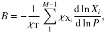 (8)where
  (9)The explicit contribution of a chemical composition gradient to the Brunt-Väisälä frequency is contained in term B. This formulation of the Brunt-Väisälä frequency, which is particularly suited for WD stars (Brassard et al. 1991), can be reduced to the usual expression of N2 in the presence of a varying composition (Cox 1980; Miglio et al. 2008). If we assume a non-degenerate and completely ionized ideal gas, which is valid in the deep interiors of MS stars such as δ Sct and γ Dor stars, Eq. (6) reduces to:
 ![Mathematical equation: \begin{equation} N^2= \frac{g^2 \rho}{P} \left[\nabla_{\rm ad}- \nabla + \nabla_{\mu} \right], \label{bv-MS} \end{equation}](/articles/aa/full_html/2017/01/aa29126-16/aa29126-16-eq95.png) (10)
(10)
where  (11)
(11)
μ being the mean molecular weight.
3. Model grid and pulsation computations
The stellar models used in this paper were calculated from the ZAMS up to the stages in which the H abundance at the core is negligible (XH ≲ 10-6), defining the terminal age main sequence (TAMS). The initial Hydrogen abundance (XH) adopted in the ZAMS varies according to the selected metallicity.
In the present analysis, we considered stellar masses between 1.2 and 2.2 M⊙ with a mass step of ΔM⋆ = 0.05 M⊙. This mass interval embraces the range of masses expected for most of the δ Sct and γ Dor stars. We consider three different values for the metallicity to generate our evolutionary sequences: Z = 0.01,0.015,0.02, thus, as mentioned before, the initial H abundance (XH) adopted in the ZAMS varies according to the selected metallicity through the relation between the metallicity and the initial He abundance (YHe): YHe = 0.245 + 2 × Z and XH + YHe + Z = 1.
In addition, we took into account the occurrence of extra-mixing episodes in the form of convective overshooting. Since overshooting is poorly constrained, we adopted four different cases: no overshooting (f = 0), moderate overshooting (f = 0.01), intermediate overshooting (f = 0.02), and extreme overshooting (f = 0.03) (see Eq. (2) for the definition of f). By varying all of these parameters we computed a large set of 21 × 3 × 4 = 252 evolutionary sequences. To have a dense grid of stellar models for each sequence (thus allowing us to carefully follow the evolution of the internal structure and also the pulsation properties of the models), the time step of LPCODE was fixed to have stellar models that differ by ~10−20 K in Teff. Thus, evolutionary sequences computed from the ZAMS to the TAMS comprise ~1500 models. All in all, we computed ~400 000 stellar models that constitute a sufficiently dense and comprehensive grid of equilibrium models representative of hybrid δ Sct-γ Dor variable stars as to ensure a consistent search for a seismological model for each target star.
For each equilibrium model we have computed the adiabatic radial (ℓ = 0) and non-radial (ℓ = 1,2,3) p and g modes with pulsation periods in the range 0.014 d ≲ Πn ≲ 3.74 d (1200 s ≲ Πn ≲ 300 000 s), thus amply embracing the range of periods usually detected in hybrid δ Sct-γ Dor stars. Models were divided into approximately 1400 mesh points and their distribution was updated at every evolutionary time-step. The number of mesh points proved to be high enough as to smoothly solve the rapidly oscillating eigenfunctions of high-radial order modes.
 |
Fig. 1 H and He fractional abundances (upper panel), the logarithm of the squared Lamb and Brunt-Väisälä frequencies, computed according to Eqs. (5) and (6), respectively (central panel), and the weight function of dipole (ℓ = 1) p- and g-modes with radial order n = 1,5,10,15,20 (lower panel), corresponding to a typical MS stellar model with M⋆ = 1.5 M⊙, L⋆ = 8.34 L⊙, Z = 0.01, f = 0.01 and τ = 1.06 Gyr. |
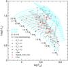 |
Fig. 2 HR diagram showing evolutionary tracks for stellar models with different masses (1.2 ≤ M⋆/M⊙ ≤ 2.2), Z = 0.015 and without overshooting (f = 0) in black, and Z = 0.01 and f = 0.03 in light blue, from the ZAMS to the TAMS. The value of the stellar mass (M⋆) is indicated for a subset of the tracks (those displayed with solid lines). Black, red, green, and blue dots correspond to the location of stellar models with M⋆/M⊙ = 1.3,1.7 and 2.1 having a central H abundance of |
Next, we describe some properties of our stellar models. We chose, in particular, a template stellar model with M⋆ = 1.5 M⊙, L⋆ = 8.34 L⊙, Z = 0.01, f = 0.01. This model is burning H at the core, and has a stellar age of τ = 1.06 Gyr. In Fig. 1, we depict some characteristics of this model. Specifically, the upper panel displays the fractional abundances of H and He in terms of normalized radius (r/R⋆). For this particular model, the central H and He abundances are 0.458 and 0.531, respectively. The model is characterized by a convective core from the stellar center (r/R⋆ = 0) to a radius r/R⋆ ~ 0.082, depicted by a grey area. We highlight that, due to overshooting, H and He are mixed up to a location somewhat beyond the boundary of the convective core, at r/R⋆ ~ 0.095. The model also has a very thin outer convection zone, barely visible in the figure, that extends from r/R⋆ ~ 0.998 to the surface (r/R⋆ = 1). The middle panel of Fig. 1 depicts a propagation diagram (see Cox 1980; Unno et al. 1989; Catelan & Smith 2015), that is, a diagram in which the Brunt-Väisälä and the Lamb frequencies (or the squares of them) are plotted against the stellar radius (or another similar coordinate). A local analysis of the pulsation equations assuming the so-called Cowling approximation (Φ′ = 0) and high-order modes (n ≫ 1), shows that p and g modes follow a dispersion relation given by: 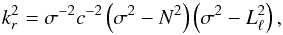 (12)
(12)
which relates the local radial wave number kr to the pulsation frequency σ (Unno et al. 1989). We note that if  or
or  , the wave number kr is real, and that if
  or
or  , then kr is purely imaginary. As we can see in the figure, there exist two propagation regions, one corresponding to the case
  , associated with p-modes, and the other in which the eigenfrequencies satisfy
  , associated with g-modes. Finally, in the lower panel of Fig. 1, we display the normalized weight functions (Eq. (A.14) of the appendix of Córsico & Althaus 2006). The weight functions indicate the regions of the star that most contribute to the period formation (Kawaler et al. 1985). The figure shows very clearly that p modes are relevant for probing the outer stellar regions, and g modes are essential for sounding the deep core regions of the star. It is precisely this property that renders hybrid δ Sct-γ Dor stars exceptional targets for asteroseismology.
In Fig. 2 we show a HR diagram displaying a subset of evolutionary sequences computed for this work. They correspond to stellar masses from 1.2 M⊙ to 2.2 M⊙, Z = 0.015, no overshooting (f = 0) in black, and Z = 0.01 and f = 0.03 in light blue. Included are the evolutionary stages comprised between the ZAMS and the TAMS. Some δ Sct, γ Dor and hybrid δ Sct-γ Dor stars (taken from Grigahcène et al. 2010)1, along with the blue and red edges of the δ Sct-γ Dor theoretical instability domains according to Dupret et al. (2005), are included for illustrative puposes.
We emphasize that, for the sake of simplicity, the impact of stellar rotation on the equilibrium models and on the pulsation spectra has been neglected for this work. Admittedly, this simplification could not be entirely valid for δ Scuti/γ Doradus stars. As a matter of fact, even at moderate rotation, the rotational splitting may completely (or almost completely) destroy the regularities in the spectra, in particular, the period spacing between consecutive high-order gravity modes of non-rotating models (see, for instance, Fig. 13 of Dziembowski et al. 1993) for the case of SPB model stars. We defer to a future publication a comprehensive study of the impact of rotation on the period spectrum of δ Scuti/γ Doradus stars.
4. The impact of extra mixing and metallicity on the pulsation properties
Below, we illustrate the effects of varying the amount of core overshooting (represented by f) and metallicity (Z) on our evolutionary models. The impact of core overshooting for different values of f on the shape and extension of evolutionary tracks is shown in the HR diagram of Fig. 3 for the case of stellar models with M⋆ = 1.70 M⊙ and Z = 0.015. As it can be seen that the occurrence of overshooting extends the incursion of the model star towards higher luminosities and lower effective temperatures, resulting ultimately in a notable broadening of the MS. This is because extra mixing promotes the existence of a larger amount of H available for burning in the stellar core. The lifetimes of stars in the MS are increased accordingly. Note that overshooting does not change the location of the ZAMS in the HR diagram, which for this particular example has log Teff ~ 3.925 and log (L⋆/L⊙) ~ 0.98.
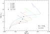 |
Fig. 3 HR diagram showing the evolutionary tracks of models with M⋆ = 1.70 M⊙, Z = 0.015 and different overshooting parameters (f = 0.00,0.01,0.02,0.03). Selected models having a central H abundance of XH ~ 0.3 marked along the tracks with black dots. |
 |
Fig. 4 HR diagram showing evolutionary tracks of models with M⋆ = 1.80 M⊙, f = 0.01 and different metallicities (Z = 0.01,0.015, and 0.02). Selected models having a central H abundance of XH ~ 0.4 marked along the tracks with black dots. |
The effects of metallicity on the evolutionary tracks is depicted in Fig. 4, where we show a HR diagram for model sequences computed assuming different metallicities (Z = 0.01,0.015 and 0.02) with M⋆ = 1.80 M⊙ and f = 0.01. It is apparent that, at variance with the effect of overshooting, when we change Z, the location of the ZAMS is notoriously affected. Indeed, reducing the metallicity from Z = 0.02 to Z = 0.015 increases ZAMS effective temperature from log Teff ~ 3.93 to log Teff ~ 3.95 (0.02 dex), and the ZAMS luminosity from log (L⋆/L⊙) ~ 1.05 to log (L⋆/L⊙) ~ 1.08 (0.03 dex). In summary, reducing the metallicity results in hotter and more luminous models. This can be understood on the basis that in spite of the fact that low-Z models experience some reduction in the CNO cycle luminosity, this dimming is compensated by the reduction of the opacity at the photosphere, which results in bluer and brighter stars (see, e.g. Hansen et al. 2004; Salaris & Cassisi 2005).
We turn now to show some p- and g-mode pulsational properties of our models. Miglio et al. (2008) have thoroughly investigated the properties of high-order g modes for stellar models with masses in the range 1−10 M⊙ in the MS and the effects of stellar mass, hydrogen abundance at the core and extra-mixing processes on the period spacing features. Therefore, we frequently make comparisons between our results and those from Miglio et al. (2008) . In Fig. 5 we show the H chemical profile (XH) at the core regions (in terms of the mass fraction coordinate −log (1−Mr/M⋆)), associated to different evolutionary stages at the MS (upper panels), and the respective squared Lamb and Brunt-Väisälä frequency runs (lower panels) corresponding to stellar models with masses M⋆ = 1.30 M⊙ (left) M⋆ = 1.70 M⊙ (center), and M⋆ = 2.10 M⊙ (right). The models were computed with Z = 0.015 and disregarding core overshooting. The location of these models is shown in Fig. 2 with coloured dots. In the upper panels of Fig. 5, the boundary of the convective core for each evolutionary stage is marked with a dot. The four evolutionary stages shown correspond to central H abundances of XH = 0.7,0.5,0.3 and 0.1. For the model with M⋆ = 1.30 M⊙ (left upper panel of Fig. 5), we obtain a growing convective core, that is, the mass of the convective core increases during part of the MS (compare with Figs. 11 and 14 of Miglio et al. 2008). As the convective core gradually grows, a discontinuity in the chemical composition occurs at its boundary, as can be appreciated from the figure.
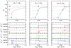 |
Fig. 5 The H abundance profile (upper panels) and the squared Brunt-Väisälä frequencies (full lines) and Lamb frequencies (dashed lines) (lower panels) for M⋆ = 1.30 M⊙ (left), M⋆ = 1.70 M⊙ (center), and M⋆ = 2.10 M⊙ (right). The four different evolutionary states displayed are clearly distinguishable from the different central abundances of H (XH = 0.7,0.5,0.3,0.1). The models, which were computed with Z = 0.015 and f = 0.00, are marked in Fig. 2 with coloured dots. |
The situation is markedly different for the models with M⋆ = 1.70 M⊙ and M⋆ = 2.10 M⊙ (centre and right upper panels of Fig. 5), characterised by a receding convective core (compare with Fig. 15 of Miglio et al. 2008). In this case, the mass of the convective core shrinks during part of the evolution at the MS. No chemical discontinuity is formed in this situation, although a chemical gradient is left at the edge of the convective core. The situation is qualitatively similar for both the 1.70 M⊙ and the 2.10 M⊙ models, the only difference being the most massive model having a slightly larger convective core (for a fixed central H abundance).
The impact of the chemical gradient at the boundary of the convective core on the Brunt-Väisälä frequency is apparent from the lower panels of Fig. 5. The specific contribution of the H/He chemical transition to N is entirely contained within the term ∇μ in Eq. (10) (or, alternatively within the term B in Eq. (6)). The feature in N induced by the chemical gradient is very narrow for the lowest-mass model shown (M⋆ = 1.30 M⊙) due to the abrupt change at the boundary of the convective core characterising this model. This feature becomes more extended for more massive models (M⋆ = 1.70 M⊙ and M⋆ = 2.10 M⊙) in response to the less steep H/He chemical transition region at the edge of the convective core.
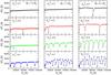 |
Fig. 6 The dipole (ℓ = 1) forward period spacing (ΔΠn) of g modes in terms of the periods Πn corresponding to the same stellar models with M⋆ = 1.30 M⊙ (left), M⋆ = 1.70 M⊙ (middle) and M⋆ = 2.10 M⊙ (right) shown in Fig. 5. The horizontal thin dashed lines correspond to the asymptotic period spacing ( |
The presence of a chemical composition gradient in the interior of a star has a strong impact on the spacing of g-mode periods with consecutive radial order, much like what happens in white dwarf pulsators that give way to the resonance phenomena called mode trapping (Brassard et al. 1992; Córsico et al. 2002). Indeed, Miglio et al. (2008) have shown in detail how deviations from a constant period spacing can yield information on the chemical composition gradient left by a convective core. In Fig. 6 we show the ℓ = 1 forward period spacing of g modes, defined as ΔΠn = Πn + 1−Πn, in terms of the pulsation periods, Πn, corresponding to the same stellar models shown in Fig. 5. We include in the plots the asymptotic period spacing,  , depicted with thin horizontal dashed lines. For a fixed abundance of H at the core (
 ), the asymptotic period spacing (and thus the mean period spacing) increases with increasing stellar mass, as predicted by Eq. (3). In fact, for more massive models the size of the convective core is larger, leading to a smaller range of integration in the integral of Eq. (3). Thus, the integral is smaller and so is larger. For a fixed stellar mass, on the other hand, the asymptotic period spacing decreases with age (lower values), because the integral increases when more evolved models are considered (see Figs. 14 and 15 of Miglio et al. 2008).
Figure 6 dramatically shows how the period spacing is affected by the presence of the composition gradient, resulting in multiple minima of ΔΠn, whose number increases as the star evolves on the MS ( diminishes). For instance, for M⋆ = 2.10 M⊙ (right panels of Fig. 5) and  , the model is just leaving the ZAMS, and there is a small step in the H profile (barely visible in the plot), which results in a peak in the Brunt-Väisälä frequency. The resulting period spacing is mostly constant, except for the presence of a strong minimum in ΔΠn (upper right panel in Fig. 6). As the star evolves and gradually consumes the H in the core, the feature in the Brunt-Väisälä frequency widens, and the edge of the convective core moves inward. When
  , the forward period spacing exhibits two strong minima. At the stage when
  , ΔΠn is no longer constant, but shows numerous minima (six in the period range displayed in the figure). This trend is further emphasised when the star is almost reaching the TAMS (
 ), as clearly depicted in the lowest right panel of Fig. 6. Our results are qualitatively similar to those of Miglio et al. (2008; see their Figs. 14 and 15). In particular, these authors have derived explicit expressions that provide the periodicity (in terms of n) of the oscillatory component in the period spacing ΔΠn and its connection with the spatial location of the sharp variation in N caused by the chemical gradient.
We also investigate the impact (if any) of the chemical gradient on the Lamb frequency which is depicted in lower panels of Fig. 5 with dashed lines. There is no apparent influence of this gradient on the Lamb frequency. However, we found that  exhibits a little bump (not visible in the plot) due to the chemical gradient. On the other hand, the Lamb frequency is lower for massive models. The forward frequency spacing for p modes corresponding to models shown in Fig. 5 is depicted in Fig. 7 for the different masses considered. In this plot, it can be seen that the asymptotic frequency spacing and Δν decrease with the evolution (i.e. lower XH values) for each considered mass.
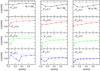 |
Fig. 7 The dipole (ℓ = 1) forward frequency spacing (Δν) of p modes in terms of the frequencies ν corresponding to the same stellar models with M⋆ = 1.30 M⊙ (left), M⋆ = 1.70 M⊙ (middle) and M⋆ = 2.10 M⊙ (right) shown in Fig. 5. The horizontal thin dashed lines correspond to the asymptotic frequency spacing ( |

Now, we describe the effects of core overshooting on the p- and g-mode pulsational properties of our models. For larger values of f (increasing overshooting), the H/He chemical interface becomes wider and less steep while shifting outwards (Fig. 8). The resulting feature in N, in turn, becomes wider and also shifts outwards, following the behaviour of the μ gradient.
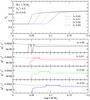 |
Fig. 8 H abundance (upper panel), and the logarithm of the squared Brunt-Väisälä and Lamb frequencies (lower panels) corresponding to the stellar models with M⋆ = 1.7 M⊙, Z = 0.015, |

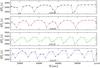 |
Fig. 9 The forward period spacing (ΔΠn) of dipole g modes vs. periods (Πn) corresponding to the same stellar models shown in Fig. 8. The asymptotic period spacing ( |
The impact of the different assumptions for core overshooting in our models on the forward period spacing of g-modes is displayed in Fig. 9. From upper to lower panels, the figure shows the forward period spacing in terms of periods for dipole g modes corresponding to increasing overshooting (f from 0 to 0.03). As it can be seen, there are several minima of ΔΠn present, whose number increases with increasing importance of overshooting. The distinct behavior of ΔΠn is due to the fact that both the location and the shape of the μ gradient are strongly modified when different values of f are adopted (see Fig. 8). Also, we note that the asymptotic period spacing slightly increases for larger f values. This is because the value of the integral in Eq. (3) diminishes for larger f. This behavior is in excellent agreement with the results of Miglio et al. (2008; their Fig. 17).
Figure 8 shows the effect of different amounts of overshooting on the Lamb frequency. There exists a very small discontinuity (small jump) in the frequency (not visible in the plot) that moves with the edge of the convective core to the outer regions, with a growing overshooting parameter, which also extends along the chemical composition gradient. This behaviour does not significantly affect the frequency spacing (see Fig. 10), whose structure remains the same for each considered overshooting parameter. However, in that figure, the asymptotic frequency spacing, depicted with a horizontal line, can be seen to slightly decrease as larger overshooting parameters are considered.
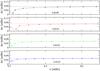 |
Fig. 10 The forward frequency spacing (Δν) of dipole p modes vs. frequency (ν) corresponding to the same stellar models shown in Fig. 8. The asymptotic frequency spacing (Δνa) is depicted with dashed lines in each case. |
In closing this section, we briefly describe the effects of different values for the metallicity Z on the pulsation properties of our MS models, while keeping stellar mass , overshooting and the central H abundance constant. We would like to highlight that alternating assumptions for the metallicity, while keeping the other parameters fixed, produces no appreciable change in the chemical profile of H and He, nor, consequently, in the Brunt-Väisälä frequency (Fig. 11). As expected, there are no significant differences in the behavior of the period spacing (ΔΠn) nor in the asymptotic period spacing ( ) of g modes, as shown in Fig. 12. The same results (not shown) are found for the frequency spacing and the asymptotic frequency spacing of p modes.
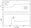 |
Fig. 11 H abundance (upper panel), and the logarithm of the squared Brunt-Väisälä frequency (lower panel) corresponding to stellar models with M⋆ = 1.80 M⊙, f = 0.01, and |

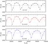 |
Fig. 12 The dipole forward period spacing (ΔΠn) of g modes in terms of the periods (Πn) corresponding to the same stellar models shown in Fig. 11. The asymptotic period spacing ( |
5. Asteroseismological analysis
In this section we will describe our asteroseismological analysis of the hybrid δ Sct-γ Dor stars KIC 11145123 (Kurtz et al. 2014), KIC 9244992 (Saio et al. 2015), HD 49434 (Brunsden et al. 2015), CoRoT 105733033 (Chapellier et al. 2012) and CoRoT 100866999 (Chapellier & Mathias 2013). As we shall see, we take fully advantage of the information contained in both the acoustic- and the gravity-mode period spectra offered by these target stars.
With the aim of searching for models that best reproduce the observed pulsation spectra of each target star, we followed two different and independent model-fitting procedures. We use the case of the HD 49434 star to illustrate these procedures. The results along with the characteristics of the other target stars are listed after this description.
HD 49434 has a visual magnitude MV = 5.74, with a FIV spectral type and effective temperature Teff = 7632 ± 126 K (Bruntt et al. 2004). This hybrid δ Sct-γ Dor star is a rapid rotator, with velocities of approximately vsini = 85.4 ± 6.6 km s-1 and a surface gravity of log g = 4.43 ± 0.20 estimated by Gillon & Magain (2006). According to Masana et al. (2006) its radius is R⋆ = 1.601 ± 0.052 R⊙ and its stellar mass is M⋆ = 1.55 ± 0.14 M⊙ (Bruntt et al. 2002). It is worth noting that the hybrid status of this star is questioned in Bouabid et al. (2009) and no gap between the frequency domains has been found in Handler (2012), probably due to its high rotation velocity, as noted by Brunsden et al. (2015). Nevertheless, in Uytterhoeven et al. (2008) and Chapellier et al. (2011) it is shown that HD 49434 has a δ Sct period region with periods in the range [1080−28 800] s, and also exhibits a γ Dor period region with periods in the range [28 800−288 000] s. Brunsden et al. (2015) propose a main period spacing of 2030.4 se for g modes. The largest amplitude period in the p-mode period range is at 9283.23 s. Table 1 summarises these stellar parameters and the observed pulsation period ranges for HD 49434.
Observational data for HD 49434.
-
Procedure 1 Step 1: we calculated the mean period spacing
 in the observed g-mode period range for
all the stellar models derived from the numerical simulations. For this star we
calculated
in the observed g-mode period range for
all the stellar models derived from the numerical simulations. For this star we
calculated  using g modes with ℓ = 1. In Fig. 13 we depict
  corresponding to the evolutionary phases from the
ZAMS to the TAMS for all the masses in our grid of models for the case with
Z =
0.01 and f = 0.01. The horizontal straight line is the
observed mean period spacing of g modes for this star
corresponding to the evolutionary phases from the
ZAMS to the TAMS for all the masses in our grid of models for the case with
Z =
0.01 and f = 0.01. The horizontal straight line is the
observed mean period spacing of g modes for this star  . As can be seen, the mean period spacing decreases
as the star evolves, thus
. As can be seen, the mean period spacing decreases
as the star evolves, thus  can be used as an indicator of the evolutionary
stage of stars and as a robust constraint in the selection of models. In this step, we
discard a large portion of the grid of models, that is, those models that do not
reproduce the observed g-mode period spacing, and we selected for each
combination of M⋆,
Z and
f,
keeping only the models that best reproduced the observed , 252 models in total.
can be used as an indicator of the evolutionary
stage of stars and as a robust constraint in the selection of models. In this step, we
discard a large portion of the grid of models, that is, those models that do not
reproduce the observed g-mode period spacing, and we selected for each
combination of M⋆,
Z and
f,
keeping only the models that best reproduced the observed , 252 models in total. 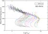
Fig. 13 Mean period spacing vs. effective temperature for models with Z = 0.01 and f = 0.01. The straight line is the observed mean period spacing for g-modes corresponding to HD 49434.
Step 2: in this step, we assume that the largest amplitude mode in the δ Sct region of the pulsation spectrum is associated to the fundamental radial mode (ℓ = 0,n = 0) or one of the low radial overtone modes (ℓ = 0, n = 1,2,3,4,...). This allows us to reduce even more the number of possible seismological models, by retaining only those models with the radial (fundamental or an overtone) mode as close as possible to the observed largest amplitude mode2. In Fig. 14 we depict the periods associated with the fundamental radial mode (n = 0) and the first radial overtone modes (n = 1,2,3) for models with Z = 0.01 and f = 0.01 selected in the previous step, that is, those models that best reproduce
. The horizontal straight line indicates the period
associated with the largest-amplitude mode in the δ Sct region of the
pulsation spectrum of HD 49434 (i.e. 9283.23 s). 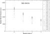
Fig. 14 Radial mode periods vs. radial order n for models selected in the previous step with Z = 0.01 and f = 0.01 for HD 49434.
Step 3: for the models selected in the previous steps, we performed a period-to-period fit to the observed p-mode periods. We calculated the quantity:
![Mathematical equation: \begin{equation} \chi^p=\sum_{i=1}^{n}{ \frac{\left[\Pi_{\rm o}^p-\Pi_{\rm c}^p\right]_i^2} {\left( \sigma_{\Pi^p}^2 \right)_i}}, \end{equation}](/articles/aa/full_html/2017/01/aa29126-16/aa29126-16-eq222.png) (13)where
(13)where  is the observed period,
  is the calculated period, σΠp is
the uncertainty associated with the observations of the considered p-mode period, and
n is
the total number of observed p-mode periods. Since no identification of the
harmonic degree is available at the outset for HD 49434, we calculated χp by searching for
the best period fit among periods of p modes with ℓ = 1,2 and
3. Accordingly, for HD
49434, takes its value from among the periods classified
as DSL (“δ Scuti like”) in the δ Sct domain in Table 3
of Brunsden et al. (2015) and is the calculated period for , which is a non-radial p mode with harmonic
degree ℓ =
1,2 or 3. All the uncertainties in the period observations were
calculated considering a conservative error of 0.01 d-1 mentioned in Brunsden et al. (2015).
Step 4: finally, in order to obtain the best-fit
model for each target star, we calculated the quantity F1 for all
the selected models in Step 2:
is the calculated period, σΠp is
the uncertainty associated with the observations of the considered p-mode period, and
n is
the total number of observed p-mode periods. Since no identification of the
harmonic degree is available at the outset for HD 49434, we calculated χp by searching for
the best period fit among periods of p modes with ℓ = 1,2 and
3. Accordingly, for HD
49434, takes its value from among the periods classified
as DSL (“δ Scuti like”) in the δ Sct domain in Table 3
of Brunsden et al. (2015) and is the calculated period for , which is a non-radial p mode with harmonic
degree ℓ =
1,2 or 3. All the uncertainties in the period observations were
calculated considering a conservative error of 0.01 d-1 mentioned in Brunsden et al. (2015).
Step 4: finally, in order to obtain the best-fit
model for each target star, we calculated the quantity F1 for all
the selected models in Step 2: ![Mathematical equation: \begin{equation} F_1=\sum_{j=1}^{N}{\frac{\left[\overline{\Delta\Pi}_n- \overline{\Delta\Pi} \right]_j^2} {\left(\sigma_{\overline{\Delta\Pi}}^2\right)_j}+ \frac{\left[\Pi_{\rm o}^r-\Pi_{\rm c}^r\right]_j^2}{(\sigma_{\Pi^r}^2)_j}+ \chi_j^p}. \label{f1} \end{equation}](/articles/aa/full_html/2017/01/aa29126-16/aa29126-16-eq230.png) (14)This quantity takes into account the differences
between the calculated and observed mean period spacing (
(14)This quantity takes into account the differences
between the calculated and observed mean period spacing ( and respectively), the difference between the
calculated radial (fundamental or an overtone) modes
and respectively), the difference between the
calculated radial (fundamental or an overtone) modes  and the observed largest amplitude mode
  , and the quantity
  calculated in the previous step, which relates the
observed set of p-mode periods with the calculated one. In this
expression, N is the number of selected models in
Step 2, that is, those that almost reproduce the observed and the largest amplitude mode.
calculated in the previous step, which relates the
observed set of p-mode periods with the calculated one. In this
expression, N is the number of selected models in
Step 2, that is, those that almost reproduce the observed and the largest amplitude mode.  is the observational uncertainty for , and σΠr is
the uncertainty corresponding to the largest-amplitude mode in the target star.
is the observational uncertainty for , and σΠr is
the uncertainty corresponding to the largest-amplitude mode in the target star. -
Procedure 2 In this procedure we considered the possibility of having radial modes among the p-mode range for the target stars. With this assumption, we exclude the direct association of the largest amplitude mode in the p-mode range with a radial mode, which is usually done for HADS stars (Catelan & Smith 2015). We performed a comparison between the observed periods in the p-mode range and the theoretical radial and non-radial p-mode periods obtained from the numerical models. Step 1 is the same as in Procedure 1, that is, we selected all models that best reproduce the observed
of g modes. Step
2: we calculated the quantity χrp for models
selected in the previous steps in order to compare the observed periods in the range
of p-mode
periods of the target star with the periods of radial and non-radial p-modes: ![Mathematical equation: \begin{equation} \chi^{rp}=\sum_{i=1}^{n}{ \frac{\left[\Pi_{\rm o}^{rp}-\Pi_{\rm c}^{rp}\right]_i^2}{(\sigma_{\Pi^{rp}}^2)_i}}, \label{chirp} \end{equation}](/articles/aa/full_html/2017/01/aa29126-16/aa29126-16-eq238.png) (15)where
(15)where  stands for the observed periods in the range of
p modes
for the target star,
stands for the observed periods in the range of
p modes
for the target star,  is the calculated period that best fits , which could be a radial or non-radial
p mode,
σΠrg
is the uncertainty associated with the observations of the considered p-mode or radial-mode
period and n is the total number of observed p-mode periods for the
target star. Step 3: we calculated the following
quantity for the models selected in Step 1:
is the calculated period that best fits , which could be a radial or non-radial
p mode,
σΠrg
is the uncertainty associated with the observations of the considered p-mode or radial-mode
period and n is the total number of observed p-mode periods for the
target star. Step 3: we calculated the following
quantity for the models selected in Step 1: ![Mathematical equation: \begin{equation} \chi^g=\sum_{i=1}^{n}{\frac{\left[\Pi_{\rm o}^g-\Pi_{\rm c}^g\right]_i^2}{(\sigma_{\Pi^g}^2)_i}} \label{chig} , \end{equation}](/articles/aa/full_html/2017/01/aa29126-16/aa29126-16-eq242.png) (16)where
(16)where  is the observed period,
  is the calculated period, σΠg is
the uncertainty associated with the observations of the considered g-mode periods and
n is
the total number of observed g-mode periods. As when calculating
χp, we looked for
the best period fit between the observed periods of g-modes and theoretical
periods with ℓ =
1,2,3. Thus, for HD 49434, takes its value from the periods in the
γ Dor
domain, classified as GDL (γ-Doradus-like) in Table 3 of Brunsden et al. (2015).
Step 4: finally, we selected the best-fit model by
calculating the quantity F2 from all models previously
selected, incorporating χrp and
χg:
is the calculated period, σΠg is
the uncertainty associated with the observations of the considered g-mode periods and
n is
the total number of observed g-mode periods. As when calculating
χp, we looked for
the best period fit between the observed periods of g-modes and theoretical
periods with ℓ =
1,2,3. Thus, for HD 49434, takes its value from the periods in the
γ Dor
domain, classified as GDL (γ-Doradus-like) in Table 3 of Brunsden et al. (2015).
Step 4: finally, we selected the best-fit model by
calculating the quantity F2 from all models previously
selected, incorporating χrp and
χg:
![Mathematical equation: \begin{equation} F_2=\sum_{j=1}^{N}{\frac{\left[\overline{\Delta\Pi}_n-\overline{\Delta\Pi} \right]_j^2}{\left(\sigma_{\overline{\Delta\Pi}}^2\right)_j}+\chi^{rp}_j+ \chi^g_j} . \end{equation}](/articles/aa/full_html/2017/01/aa29126-16/aa29126-16-eq248.png) (17)It is worth mentioning that, for HD 49434, we did not
include in χp the period
classified as DLS with the largest amplitude. Instead, we assumed that it is a period
corresponding to a radial mode in order to perform Step 2 of
Procedure 1. In Eq. (15) ofProcedure 2
we included the aforementioned largest-amplitude mode, that is, we considered the
possibility of having radial modes in the δ Sct domain. Table 2 resumes the characteristics of the models selected for each
procedure. Table 2
(17)It is worth mentioning that, for HD 49434, we did not
include in χp the period
classified as DLS with the largest amplitude. Instead, we assumed that it is a period
corresponding to a radial mode in order to perform Step 2 of
Procedure 1. In Eq. (15) ofProcedure 2
we included the aforementioned largest-amplitude mode, that is, we considered the
possibility of having radial modes in the δ Sct domain. Table 2 resumes the characteristics of the models selected for each
procedure. Table 2Best-fit models for HD 49434.
Now we give details of these procedures for the four additional target stars.
5.1. KIC 11145123
KIC 11145123, also known as the “Holy Grail”, is a late A δ Sct-γ Dor hybrid star observed by the Kepler mission and extensively studied by Kurtz et al. (2014). From the Kepler Input Catalogue (KIC) revised photometry (Huber et al. 2014), its effective temperature is 8050 ± 200 K and its surface gravity is log g = 4.0 ± 0.2 (cgs units). It also has a Kepler magnitude Kp = 13. The p-mode periods present in KIC 11145123 are in the range [3536.75−5160.67] s and the g-mode period range is [42 255.53−71 430] s. The complete list of p- and g-mode frequencies are in Tables 2 and 3, respectively, of Tkachenko et al. (2013). The mean period spacing for g modes is  s and the largest amplitude mode in the δ Sct region of the pulsation spectrum has a period of 4810.69 s. Table 3 resumes these stellar parameters and the observed pulsation-period range for KIC 11145123.
Observational data for KIC 11145123.
In Step 1 of Procedure 1, in the γ Dor domain was calculated using only pulsation g modes with harmonic degree ℓ = 1, since KIC 11145123 shows only triplets in the γ Dor domain. Figure 15 shows the mean period spacing for models with Z = 0.01 and f = 0.
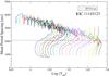 |
Fig. 15 Mean period spacing vs. effective temperature for models with Z = 0.01 and f = 0. The straight line is the observed mean period spacing for g-modes for the case of KIC 11145123. |
We performed Step 2 of Procedure 1. Figure 16 depicts the radial mode periods (the fundamental and the overtones) for models with Z = 0.01 and f = 0, selected from the previous step.
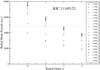 |
Fig. 16 Radial mode periods vs. radial order n for models selected in Step 1 with Z = 0.01 and f = 0, corresponding to KIC 11145123. |
We modified Step 3 , given that this target star has modes classified with ℓ = 1 and ℓ = 2, computing two quantities: χ1 and χ2, for models with p-mode periods with ℓ = 1 and ℓ = 2 respectively, since KIC 11145123 exhibits three rotational quintuplets (ℓ = 2) and five rotational triplets (ℓ = 1). The expression for these quantities is given by:  (18)
(18)
where N is the total number of observed p-mode periods with ℓ = 1 for j = 1 and ℓ = 2 for j = 2.  is the observed p-mode period,
  is the closest period to between those with ℓ = 1 for j = 1 and ℓ = 2 for j = 2 and σΠ is the uncertainty associated with
  . Thus, χp is given by χp = χ1 + χ2.
As with HD 49434, we included a period-to-period fit for the g-modes. We used the g-mode periods listed in Table 3 of Kurtz et al. (2014) in order to calculate χg and thus obtained two different models.
Procedure 2 was not performed for this star since all its frequencies in the δ Sct region were classified as p-mode with their corresponding harmonic degree and we believe this classification is correct.
Best-fit models for KIC 11145123 with Procedure 1.
In Table 4, the characteristics of the asteroseismological models selected for KIC 11145123 according Procedure 1 with and without a g-mode period-to-period fit are shown. Two different seismological models were obtained meaning that individual g-mode period fits play an important role in the modelling of this star. Comparing our models with those obtained in Kurtz et al. (2014) with M⋆ = 1.40 M⊙,1.46 M⊙ and 2.05 M⊙ and Z = 0.01 and 0.014, we note some differences in these values, possibly due to the fact that we did not consider atomic diffusion in our simulations (the Brunt-Väisälä frequency is modified by this physical process). Nevertheless, our best-fit models are both in the TAMS overall contraction phase in good agreement with those obtained by Kurtz et al. (2014) and also have a metallicity consistent with the hypothesis that this star could be a SX Phe star. Note that neither model aptly reproduces the reported effective temperature for this star.
5.2. KIC 9244992
This star, observed by the Kepler Mission, has an effective temperature of Teff = 6900 ± 300 K and its surface gravity is log g = 3.5 ± 0.4 according to the KIC revised photometry (Huber et al. 2014). A recent study (Nemec et al. 2015) obtains 3.8388 ≤ log Teff ≤ 3.8633 K and 3.5 ≤ log g ≤ 4.0 and a rotational velocity of vsin(i) ≤ 6 km s-1 which indicates KIC 9244992 is a slow rotator. The p- and g-mode period ranges for this star are [4689.89−7017.28] s and [54 000−96 000] s, respectively. It shows a radial mode with a period equal to 7001.97 s and its mean period spacing for g-modes is  s. The complete lists of g- and p-mode periods are shown in Tables 1 and 3, respectively, of Saio et al. (2015). Table 5 summarises these stellar parameters and the observed pulsational periods range for KIC 9244992.
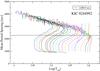 |
Fig. 17 Mean period spacing of g modes vs. effective temperature for models with Z = 0.02 and f = 0. The straight horizontal line is the observed mean period spacing for g-modes corresponding to KIC 9244992. |
We calculated the mean period spacing in the observed g-mode period range () using models with harmonic degree ℓ = 1. In Fig. 17 we depict the calculated vs. log Teff for models with Z = 0.02 and f = 0 and different values of stellar mass.
Observational data for KIC 9244992.
Next, we performed Step 2 of Procedure 1. Figure 18 shows the radial mode periods for the selected models in the previous step with Z = 0.02 and f = 0.
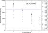 |
Fig. 18 Radial mode periods vs. radial order n for the models selected in the previous step with Z = 0.02 and f = 0, corresponding to KIC 9244992. |
KIC 9244992 has six p-mode frequencies with ℓ = 1 and four without assigned harmonic degree, according to the classification in Saio et al. (2015). Thus, we modified Step 3 with the aim of including this classification. We calculated two quantities. On one hand, we assess χ1, which compares ν2, ν7, ν8, ν9, ν11 and ν6 () from Table 3 of Saio et al. (2015) with the calculated p-mode periods with harmonic degree ℓ = 1, by means of the following expression:
![Mathematical equation: \begin{equation} \chi_{1}=\sum_{i=1}^{6}{ \frac{\left[\Pi^p_{\rm o}-\Pi^p_{\rm c}\right]_i^2}{(\sigma_{1}^2)_i}}, \label{chi1} \end{equation}](/articles/aa/full_html/2017/01/aa29126-16/aa29126-16-eq295.png) (19)
(19)
where σ1 is the uncertainty associated with the observed p-mode frequencies with ℓ = 1. On the other hand, we compute χ123, which compares the frequencies without an assigned harmonic degree () with those p-mode frequencies calculated with ℓ = 1,2 and 3 (), that is, we search for the best period-fit among the non-radial p modes with ℓ = 1,2 and 3. Thus, χ123 is defined as:
![Mathematical equation: \begin{equation} \chi_{123}=\sum_{i=1}^{4}{ \frac{\left[\Pi^p_{\rm o}-\Pi^p_{\rm c}\right]_i^2}{\left(\sigma_{123}^2\right)_i}} \label{chi123} , \end{equation}](/articles/aa/full_html/2017/01/aa29126-16/aa29126-16-eq299.png) (20)
(20)
where σ123 is the uncertainty associated with the observations of the considered . Thus, χp has the expression: χp = χ1 + χ123.
Procedure 2 was not performed since all the p-mode periods are classified with their corresponding harmonic degree.
In Table 6 we show the characteristics of the best-fit model selected for KIC 9244992. Also in this case, we added a g-mode period-to-period fit in Eq. (14), considering models with ℓ = 1 in order to obtain χg, since the target star has only rotational triplets in the g-mode period range. The same model was obtained, meaning that including a g-mode period-to-period fit does not affect the selection of the model. In Saio et al. (2015) the authors propose a model with M⋆ = 1.45 M⊙, Z = 0.01 and f = 0.005. Our 2.1 M⊙ best-fit model is more massive, does not have overshooting in the core and has higher metallicity (Z = 0.02). Thus, our results do not indicate that this star is actually a SX Phe star. In addition, the log g = 3.8 obtained is in good agreement with the spectroscopic study referenced by Saio et al. (2015), but we note that our model has a higher effective temperature (around 900 K). This could be due to the fact that we include in our procedures only the dominant frequencies, and not all the detected ones, as was the case in Saio et al. (2015). Despite these differences, our best-fit model for KIC 9244992 is also at the end of the MS stage.
Best-fit model for KIC 9244992.
5.3. CoRoT 105733033
According to measurements provided by the EXODAT database, CoRoT 105733033 has a A5V spectral type with magnitude V = 12.8 and an effective temperature of 8000 K. This star is a good example of a hybrid pulsator since it shows g and p modes in two clearly distinct frequency domains. Chapellier et al. (2012) divided the CoRoT 105733033 periods into two domains: the γ Dor domain with periods in the range [21 600−345 600] s and the δ Sct domain with periods in the range [1362.77−8554.45] s, with the largest-amplitude mode in the δ Sct domain having a period 9816.08 s, and a mean period spacing of g modes of 2655.936 s. To perform our calculations we used a g-mode period range of [59 961.6−137 635.2] s. Table 7 summarises these stellar parameters and the observed pulsation-period ranges for CoRoT 105733033.
Observational data for CoRoT 105733033.
In Fig. 19 we display the variation of the mean period spacing in the g-mode range with the effective temperature for models with Z = 0.015 and f = 0.03. We calculated using modes with ℓ = 1. Next, we performed Step 3 of Procedure 1. Figure 20 shows the radial modes for selected models with Z = 0.015 and f = 0.03.
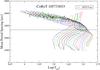 |
Fig. 19 Mean period spacing vs. effective temperature for models with Z = 0.015 and f = 0.03. The straight line is the observed mean period spacing for g modes of CoRoT 105733033. |
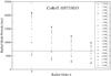 |
Fig. 20 Radial mode periods vs. radial order n for models selected in the previous step with Z = 0.015 and f = 0.03. |
The complete list of the detected frequencies can be found in Table 1 of Chapellier et al. (2012). There are 444 frequencies classified as δ Sct-type or γ Dor-type shown in the aforementioned table. We performed our calculation dismissing all kinds of combination frequencies. Since none of the p- or g-mode periods have an assigned harmonic degree, we calculated χp and χg searching for the best period fit among modes with ℓ = 1,2 and 3. As with HD 49434, the largest-amplitude mode (classified as F in Table 1 of Chapellier et al. (2012)) was dismissed in the calculation of χp in Procedure 1, but included in the calculation of χrp in Procedure 2.
In Table 8 we show the main characteristics of the asteroseismological models selected for CoRoT 105733033. So far, no asteroseismological model has been proposed for this star, and its physical characteristics are quite uncertain. Here, we present the first asteroseismic model of this star (parameters displayed in Table 8). As previously mentioned, we performed two different procedures and obtained two different models, depicted in Fig. 23, both reaching the TAMS. Again, we calculated χg in order to add it in F1 for Procedure 1 and obtained the same model (the one with 1.75 M⊙) and another different model from Procedure 2 (the one with 1.85 M⊙). This means that the best-fit model selected persists when we consider a period-to-period fit of g-modes, but changes when we include the possibility of having radial modes between the frequencies detected in the δ Sct domain. Anyway, both models are before the TAMS, and have the same overshooting parameter and similar effective temperatures and surface gravities.
Best-fit models for CoRoT 105733033.
5.4. CoRoT 100866999
This star is an eclipsing binary system with a pulsating primary star compatible with an A7-F0 spectral type and a secondary star with a G5-K0 spectral type (Chapellier & Mathias 2013). From the eclipsing curve fit, these authors found a stellar mass of (1.8 ± 0.2) M⊙, a radius of (1.9 ± 0.2) R⊙, a surface gravity of log g = 4.1 ± 0.1 and an effective temperature of (7300 ± 250) K for the primary star. For the secondary star, a stellar mass of (1.1 ± 0.2)M⊙, a radius of (0.9 ± 0.2) R⊙, a surface gravity of log g = 4.6 ± 0.1 and an effective temperature of (5400 ± 430) K was found. The pulsating primary star has two well-separated δ Sct and γ Dor period domains. The g-mode period range of this star is [23 736−288 000] s and the p-mode periods are in the range [2544.16−5927.14] s. CoRoT 100866999 has a mean period spacing of g modes equal to 3017.952 sec and presents the largest-amplitude mode in the δ Sct period range at 5088.24 s. Table 9 summarises these stellar parameters and the observed pulsation period ranges for CoRoT 100866999.
Observational data for CoRoT 100866999.
We calculated using modes with ℓ = 1, since ΔΠ separation is compatible with ℓ = 1g modes, as mentioned by Chapellier & Mathias (2013). Figure 21 depicts the calculated mean period spacing for models with Z = 0.02 and f = 0.
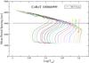 |
Fig. 21 Mean period spacing of g modes vs. effective temperature for models with Z = 0.02 and f = 0. The horizontal straight line is the observed mean period spacing for g-modes of CoRoT 100866999. |
For Step 2 of Procedure 1 we adopted the largest-amplitude mode frequency as the radial fundamental mode, that is, 5088.249 s. The radial-mode periods for the models selected in the previous step with Z = 0.02 and f = 0 are depicted in Fig. 22. As previously, we only selected models whose fundamental or overtone radial mode is 100 s or less away from the largest-amplitude mode detected in CoRoT 100866999.
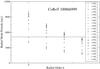 |
Fig. 22 Radial mode periods vs. radial order n for models selected in the previous step with Z = 0.02 and f = 0, corresponding to CoRoT 100866999. |
Again, we calculated χp and χg in the same way as for HD 49434 and CoRoT 105733033, since there is no harmonic degree classification for any of the detected mode periods. This fact allowed us to perform Procedure 2. In Table 10, we display the characteristics of the models selected for CoRoT 100866999.
Best-fit model for CoRoT 100866999.
We obtained one model from Procedure 1 with and without considering χg in F1 and a different model from Procedure 2. The one obtained from Procedure 1 with 1.55 M⊙ is located before the “knee” of the MS. The other one, obtained with Procedure 2, has 2.10 M⊙ and it is near the TAMS. Both models have Z = 0.02. These values are close to those obtained in Chapellier & Mathias (2013) from the eclipsing curve fit for the primary star (1.8 ± 0.2 M⊙).
With the aim of quantifying our model selections, in Table 11 we show the differences between the observed and the computed period spacing of g modes, δ(ΔΠ); the observed and computed period of the highest-amplitude radial mode, δ(Πr); and the quantities σp, σg and σrp defined as: 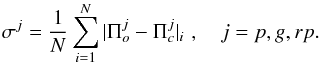 (21)
(21)
Note that σrp has been computed only for target stars with no clear mode identification, as Procedure 2 requires.
The O−C differences of each method and target star.
6. Summary and conclusions
Here we present a detailed asteroseismic study of five hybrid δ Scuti-γ Doradus pulsating stars, aimed at deriving their fundamental stellar parameters. To this end we built a huge grid of stellar models, covering the evolution of low-mass stars from the ZAMS to the TAMS, varying the stellar mass, the metallicity and the amount of core overshooting (see Sect. 3). We employed the observational data of the detected periods reported in Kurtz et al. (2014) for KIC 11145123, Saio et al. (2015) for KIC 9244992, Brunsden et al. (2015) for HD 49434, Chapellier et al. (2012) for CoRoT 105733033, and Chapellier & Mathias (2013) for CoRoT 100866999. We were able to obtain the fundamental parameters of the target stars by performing two different procedures, which fully exploit the simultaneous presence of p and g modes (and also presumably radial modes) for this kind of pulsating star.
For Procedure 1 we used three constraints to find the best-fit seismological models: (1) the mean period spacing of high-order g modes; (2) the largest amplitude mode in the δ Sct period domain, to which we associate a radial mode; and (3) a period-to-period fit of the individual p modes. Furthermore, in this case we explore the effect of adding a period-to-period fit of g modes in the selection of the best-fit model. Finally in Procedure 2 we again used the mean period spacing of g modes and, in addition, a period-to-period fit between the frequencies detected in the δ Sct domain and those calculated for models with p-mode periods and also (simultaneously) radial-mode periods. It is worth mentioning that these procedures do not depend on the reported spectroscopic information of the target stars, such as the effective temperature.
Below we summarise the results obtained for each star:
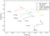 |
Fig. 23 HR diagram showing the asteroseismological models found and the respective evolutionary tracks for each target star. |
-
KIC 11145123: two different seismological models were obtained from Procedure 1 with and without including χg in F1(see Table 4). This means that individual g-mode period fits play an important role in the modelling of this star. Comparing our models with those obtained in Kurtz et al. (2014), we note some differences in the mass and the metallicity, possibly due to the fact that we did not consider atomic diffusion in our simulations, the Brunt-Väisälä frequency being modified by this physical process, and neglected rotation in our pulsation modelling. Nevertheless, our best-fit models are both in the TAMS overall contraction phase, in good agreement with those obtained in Kurtz et al. (2014), and also have a metallicity consistent with the hypothesis that this star could be a SX Phe star. Note that neither model aptly reproduces the reported effective temperature for this star.
-
KIC 9244992: the characteristics of the model obtained for this star are shown in Table 6. In this case, we obtained the same best-fit model with and without including χg in Procedure 1. This means that including a g-mode period-to-period fit does not affect the selection of the model. Our 2.1 M⊙ best-fit model is more massive that the one proposed in Saio et al. (2015) of 1.45 M⊙. Also, our model does not have overshooting in the core and has higher metallicity (Z = 0.02). Thus, our results do not indicates that this star is actually a SX Phe star. In addition, the log g = 3.8 obtained is in good agreement with the spectroscopic study cited in Saio et al. (2015), however we note that our model has a higher effective temperature. Despite these differences, our best-fit model for KIC 9244992 is also at the end of the MS stage.
-
HD 49434: we performed Procedure 2 for this star since the mode classification is not conclusive and therefore the existence of radial modes in the δ Sct region cannot be discarded. We obtained one model with Z = 0.01 and f = 0.01 from Procedure 1, and another model with Z = 0.015 and f = 0.03 from Procedure 2. Both models have the same mass, 1.75 M⊙. One of them has f = 0.03 and is near the TAMS, and the other one has f = 0.01 and is before the evolutionary “knee” where the overall contraction phase begins (see Fig. 23). One of the main characteristics of this star is that it is a rapid rotator, and so it does not show a clear gap between the δ Sct and γ Dor pulsation spectra regions. It is possible, as mentioned by Brunsden et al. (2015), that the absence of the gap is due precisely to rotational splitting of high-degree p modes. If this is the case, correct mode identification is necessary since our methodology strongly depends on this. On the other hand it is worth mentioning that adding a period-to-period fit for the g-modes does not affect the selection of the best-fit model since we obtained the same models including χg in Procedure 1. The selection of another model when we include the possibility of having radial modes in the δ Sct period domain indicates a necessity for correct mode classification.
-
CoRoT 105733033: one of the remarkable characteristics of this star is the richness of its pulsational spectra. As mentioned previously, it is possible to observe a clear distinction between low- and high-frequency regions in this star, which may be the consequence of a relatively low angular rotation (Chapellier et al. 2012). More spectroscopic data are required to confirm this hypothesis. So far, no asteroseismological model has been proposed for this star, and its physical characteristics are uncertain. In this paper, we present the first asteroseismic model (see Table 8). As previously mentioned, we performed three different procedures and obtained two different models, both at the overall contraction phase (Fig. 23). Again, from Procedure 1 when we include χg we obtained the same model (one with 1.75 M⊙) and another different model from Procedure 2 (the one with 1.85 M⊙). This means that the best-fit model selected persists when we consider a period-to-period fit of g-modes, but changes when we include the possibility of having radial modes among the frequencies detected in the δ Sct domain. Nonetheless, both models are at the overall contraction phase, and have the same overshooting parameter and similar effective temperature and surface gravity.
-
CoRoT 100866999: we obtained one model from Procedure 1 and a different model from Procedure 2. The one obtained with Procedure 1 is 1.55 M⊙ and is located before the evolutionary “knee” of the MS. The other one, obtained with Procedure 2, has 2.10 M⊙ and is on the overall contraction phase. Both models have Z = 0.02. Comparing these mass values with the ones obtained in Chapellier & Mathias (2013) from the eclipsing curve fit, we can see that ours masses are close to those calculated for the primary star (1.8 ± 0.2 M⊙).
In summary, we obtained the first reliable asteroseismological models representative of five δ Sct-γ Dor hybrid stars by means of grid-based modelling. These asteroseismological models result from different criteria of model selection, in which we take full advantage of the richness of periods that characterises the pulsation spectra of this kind of star. For four out the five stars analysed, we obtained the same asteroseismological model from Procedure 1 including or not a period-to-period fit of the g modes. In the cases when it was possible to apply Procedure 2, we obtained a different model from this approach. The true seismic model for a given target star must reproduce not only observed frequencies and regularities in the frequency spectra, but also frequency ranges of observed oscillations as ranges of pulsationally unstable radial and non-radial modes. We considered only adiabatic oscillations in our approach, and a detailed stability analysis of oscillations, which is beyond the scope of the present work, will be addressed in a future paper. Clearly, more theoretical work in the frame of this issue (like non-adiabatic stability computations), and also in other topics, for instance, the inclusion of the effects of rotation on the pulsation periods and substantial improvement of mode identification, will help us to break the degeneracy of the asteroseismological solutions.
Other larger and recent samples can be found in Bradley et al. (2015), Balona et al. (2015).
In practice we adopted an arbitrary difference of ~100 s.
Acknowledgments
We wish to thank our anonymous referee for the constructive comments and suggestions that greatly improved the original version of the paper. The complete grid of stellar models used in this paper was computed with the calculus cluster of the “Instituto de Física de Líquidos y Sistemas Biológicos” which belong to the “National System for High Performance Computing” (SNCAD) of the Ministry of Science, Technology and Productive Innovation-Argentina. Part of this work was supported by AGENCIA through the Programa de Modernización Tecnolǵica BID 1728/OC-AR, and by the PIP 112-200801-00940 grant from CONICET. This research has made use of NASA Astrophysics Data System.
References
- Aerts, C., Christensen-Dalsgaard, J., & Kurtz, D. W. 2010, Asteroseismology, Astron. Astrophys. Lib. (Springer) [Google Scholar]
- Althaus, L. G., Serenelli, A. M., Córsico, A. H., & Montgomery, M. H. 2003, A&A, 404, 593 [NASA ADS] [CrossRef] [EDP Sciences] [Google Scholar]
- Althaus, L. G., Serenelli, A. M., Panei, J. A., et al. 2005, A&A, 435, 631 [NASA ADS] [CrossRef] [EDP Sciences] [Google Scholar]
- Althaus, L. G., Córsico, A. H., Isern, J., & García-Berro, E. 2010, A&ARv, 18, 471 [NASA ADS] [CrossRef] [Google Scholar]
- Althaus, L. G., García-Berro, E., Isern, J., Córsico, A. H., & Miller Bertolami, M. M. 2012, A&A, 537, A33 [NASA ADS] [CrossRef] [EDP Sciences] [Google Scholar]
- Althaus, L. G., Miller Bertolami, M. M., & Córsico, A. H. 2013, A&A, 557, A19 [NASA ADS] [CrossRef] [EDP Sciences] [Google Scholar]
- Antoci, V., Handler, G., Campante, T. L., et al. 2011, Nature, 477, 570 [NASA ADS] [CrossRef] [PubMed] [Google Scholar]
- Arellano Ferro, A., Ahumada, J. A., Calderón, J. H., & Kains, N. 2014, Mex. Astron. Astrofis., 50, 307 [Google Scholar]
- Baglin, A., Auvergne, M., Barge, P., et al. 2009, in IAU Symp. 253, eds. F. Pont, D. Sasselov, & M. J. Holman,71 [Google Scholar]
- Balona, L. A. 2010, Challenges In Stellar Pulsation (Bentham Publishers) [Google Scholar]
- Balona, L. A., Krisciunas, K., & Cousins, A. W. J. 1994, MNRAS, 270, 905 [NASA ADS] [CrossRef] [Google Scholar]
- Balona, L. A., Daszyńska-Daszkiewicz, J., & Pamyatnykh, A. A. 2015,MNRAS, 452, 3073 [Google Scholar]
- Bognár, Z., Lampens, P., Frémat, Y., et al. 2015, A&A, 581, A77 [NASA ADS] [CrossRef] [EDP Sciences] [Google Scholar]
- Bouabid, M.-P., Montalbán, J., Miglio, A., et al. 2009, in AIP Conf. Ser. 1170, eds. J. A. Guzik & P. A. Bradley,477 [Google Scholar]
- Bradley, P. A., Guzik, J. A., Miles, L. F., et al. 2015, AJ, 149, 68 [NASA ADS] [CrossRef] [Google Scholar]
- Brassard, P., Fontaine, G., Wesemael, F., Kawaler, S. D., & Tassoul, M. 1991, ApJ, 367, 601 [NASA ADS] [CrossRef] [Google Scholar]
- Brassard, P., Fontaine, G., Wesemael, F., & Hansen, C. J. 1992, ApJS, 80, 369 [NASA ADS] [CrossRef] [Google Scholar]
- Brunsden, E., Pollard, K. R., Cottrell, P. L., et al. 2015, MNRAS, 447, 2970 [NASA ADS] [CrossRef] [Google Scholar]
- Bruntt, H., Catala, C., Garrido, R., et al. 2002, A&A, 389, 345 [NASA ADS] [CrossRef] [EDP Sciences] [Google Scholar]
- Bruntt, H., Bikmaev, I. F., Catala, C., et al. 2004, A&A, 425, 683 [NASA ADS] [CrossRef] [EDP Sciences] [Google Scholar]
- Campbell, W. W., & Wright, W. H. 1900, ApJ, 12, 254 [NASA ADS] [CrossRef] [Google Scholar]
- Catelan, M., & Smith, H. A. 2015, Pulsating Stars (Wiley-VCH) [Google Scholar]
- Chapellier, E., & Mathias, P. 2013, A&A, 556, A87 [NASA ADS] [CrossRef] [EDP Sciences] [Google Scholar]
- Chapellier, E., Rodríguez, E., Auvergne, M., et al. 2011, A&A, 525, A23 [NASA ADS] [CrossRef] [EDP Sciences] [Google Scholar]
- Chapellier, E., Mathias, P., Weiss, W. W., Le Contel, D., & Debosscher, J. 2012, A&A, 540, A117 [NASA ADS] [CrossRef] [EDP Sciences] [Google Scholar]
- Charbonnel, C., & Zahn, J.-P. 2007, A&A, 467, L15 [NASA ADS] [CrossRef] [EDP Sciences] [Google Scholar]
- Chevalier, C. 1971, A&A, 14, 24 [NASA ADS] [Google Scholar]
- Civelek, R., Kızıloǧlu, N., & Kırbıyık, H. 2001, AJ, 122, 2042 [NASA ADS] [CrossRef] [Google Scholar]
- Civelek, R., Kızıloğlu, N., & Kırbıyık, H. 2003, A&A, 411, 503 [NASA ADS] [CrossRef] [EDP Sciences] [Google Scholar]
- Córsico, A. H., & Althaus, L. G. 2006, A&A, 454, 863 [NASA ADS] [CrossRef] [EDP Sciences] [Google Scholar]
- Córsico, A. H., & Althaus, L. G. 2014a, A&A, 569, A106 [NASA ADS] [CrossRef] [EDP Sciences] [Google Scholar]
- Córsico, A. H., & Althaus, L. G. 2014b, ApJ, 793, L17 [NASA ADS] [CrossRef] [Google Scholar]
- Córsico, A. H., & Benvenuto, O. G. 2002, Ap&SS, 279, 281 [NASA ADS] [CrossRef] [Google Scholar]
- Córsico, A. H., Althaus, L. G., Benvenuto, O. G., & Serenelli, A. M. 2001, A&A, 380, L17 [NASA ADS] [CrossRef] [EDP Sciences] [Google Scholar]
- Córsico, A. H., Althaus, L. G., Benvenuto, O. G., & Serenelli, A. M. 2002, A&A, 387, 531 [NASA ADS] [CrossRef] [EDP Sciences] [Google Scholar]
- Córsico, A. H., Althaus, L. G., Montgomery, M. H., García-Berro, E., & Isern, J. 2005, A&A, 429, 277 [NASA ADS] [CrossRef] [EDP Sciences] [Google Scholar]
- Córsico, A. H., Althaus, L. G., Kepler, S. O., Costa, J. E. S., & Miller Bertolami, M. M. 2008, A&A, 478, 869 [NASA ADS] [CrossRef] [EDP Sciences] [Google Scholar]
- Córsico, A. H., Althaus, L. G., Miller Bertolami, M. M., et al. 2012, MNRAS, 424, 2792 [NASA ADS] [CrossRef] [Google Scholar]
- Cox, J. P. 1980, in Theory of stellar pulsation, (Princetion University Press), 174 [Google Scholar]
- Dupret, M.-A., Grigahcène, A., Garrido, R., Gabriel, M., & Scuflaire, R. 2004, A&A, 414, L17 [NASA ADS] [CrossRef] [EDP Sciences] [Google Scholar]
- Dupret, M.-A., Grigahcène, A., Garrido, R., Gabriel, M., & Scuflaire, R. 2005, A&A, 435, 927 [NASA ADS] [CrossRef] [EDP Sciences] [Google Scholar]
- Dziembowski, W. A. 1971, Acta Astron., 21, 289 [NASA ADS] [Google Scholar]
- Dziembowski, W. A., Moskalik, P., & Pamyatnykh, A. A. 1993, MNRAS, 265, 588 [NASA ADS] [Google Scholar]
- Ferguson, J. W., Alexander, D. R., Allard, F., et al. 2005, ApJ, 623, 585 [NASA ADS] [CrossRef] [Google Scholar]
- Gai, N., Basu, S., Chaplin, W. J., & Elsworth, Y. 2011, ApJ, 730, 63 [NASA ADS] [CrossRef] [Google Scholar]
- Gillon, M., & Magain, P. 2006, A&A, 448, 341 [NASA ADS] [CrossRef] [EDP Sciences] [Google Scholar]
- Grevesse, N., & Noels, A. 1993, in Origin and Evolution of the Elements, eds. N. Prantzos, E. Vangioni-Flam, & M. Casse (Cambridge University Press), 15 [Google Scholar]
- Grigahcène, A., Dupret, M.-A., Gabriel, M., Garrido, R., & Scuflaire, R. 2005, A&A, 434, 1055 [NASA ADS] [CrossRef] [EDP Sciences] [Google Scholar]
- Grigahcène, A., Antoci, V., Balona, L., et al. 2010, ApJ, 713, L192 [NASA ADS] [CrossRef] [Google Scholar]
- Guzik, J. A., Kaye, A. B., Bradley, P. A., Cox, A. N., & Neuforge, C. 2000, ApJ, 542, L57 [NASA ADS] [CrossRef] [Google Scholar]
- Handler, G. 2009, MNRAS, 398, 1339 [NASA ADS] [CrossRef] [Google Scholar]
- Handler, G. 2012, Progress in Solar/Stellar Physics with Helio- and Asteroseismology, eds. H. Shibahashi, M. Takata, & A. E. Lynas-Gray, ASP Conf. Ser., 462, 111 [Google Scholar]
- Hansen, C. J., Kawaler, S. D., & Trimble, V. 2004, Stellar interiors: physical principles, structure, and evolution, (New York: Springer-Verlag) [Google Scholar]
- Hareter, M., Reegen, P., Miglio, A., et al. 2010, ArXiv e-prints [arXiv:1007.3176] [Google Scholar]
- Hekker, S., & Ball, W. H. 2014, A&A, 564, A105 [NASA ADS] [CrossRef] [EDP Sciences] [Google Scholar]
- Henry, G. W., & Fekel, F. C. 2005, AJ, 129, 2026 [NASA ADS] [CrossRef] [Google Scholar]
- Herwig, F. 2000, A&A, 360, 952 [NASA ADS] [Google Scholar]
- Herwig, F., Bloecker, T., Schoenberner, D., & El Eid, M. 1997, A&A, 324, L81 [NASA ADS] [Google Scholar]
- Herzberg, W., Uytterhoeven, K., & Roth, M. 2012, Astron. Nachr., 333, 1077 [NASA ADS] [CrossRef] [Google Scholar]
- Huber, D., Silva Aguirre, V., Matthews, J. M., et al. 2014, ApJS, 211, 2 [NASA ADS] [CrossRef] [Google Scholar]
- Iglesias, C. A., & Rogers, F. J. 1996, ApJ, 464, 943 [NASA ADS] [CrossRef] [Google Scholar]
- Kawaler, S. D., Winget, D. E., & Hansen, C. J. 1985, ApJ, 295, 547 [NASA ADS] [CrossRef] [Google Scholar]
- Kaye, A. B., Handler, G., Krisciunas, K., Poretti, E., & Zerbi, F. M. 1999, PASP, 111, 840 [NASA ADS] [CrossRef] [Google Scholar]
- Keen, M. A., Bedding, T. R., Murphy, S. J., et al. 2015, MNRAS, 454, 1792 [NASA ADS] [CrossRef] [Google Scholar]
- King, H., Matthews, J. M., Row, J. F., et al. 2006, Comm. Asteroseismol., 148, 28 [Google Scholar]
- Kippenhahn, R. 1967, in Proc. of Colloquium on Late-Type Stars, ed. M. Hack, 319 [Google Scholar]
- Kippenhahn, R., Weigert, A., & Weiss, A. 2012, in Stellar Structure and Evolution Astron. Astrophys. Lib. (Berlin, Heidelberg: Springer-Verlag) [Google Scholar]
- Koch, D. G., Borucki, W. J., Basri, G., et al. 2010, ApJ, 713, L79 [NASA ADS] [CrossRef] [Google Scholar]
- Kurtz, D. W., Saio, H., Takata, M., et al. 2014, MNRAS, 444, 102 [NASA ADS] [CrossRef] [Google Scholar]
- Kurtz, D. W., Hambleton, K. M., Shibahashi, H., Murphy, S. J., & Prša, A. 2015, MNRAS, 446, 1223 [NASA ADS] [CrossRef] [Google Scholar]
- Lee, Y.-H., Kim, S. S., Shin, J., Lee, J., & Jin, H. 2008, PASJ, 60, 551 [NASA ADS] [Google Scholar]
- Lenz, P., Pamyatnykh, A. A., Breger, M., & Antoci, V. 2008, A&A, 478, 855 [NASA ADS] [CrossRef] [EDP Sciences] [Google Scholar]
- Masana, E., Jordi, C., & Ribas, I. 2006, A&A, 450, 735 [NASA ADS] [CrossRef] [EDP Sciences] [Google Scholar]
- Miglio, A., Montalbán, J., Noels, A., & Eggenberger, P. 2008, MNRAS, 386, 1487 [NASA ADS] [CrossRef] [Google Scholar]
- Miller Bertolami, M. M., & Althaus, L. G. 2006, A&A, 454, 845 [NASA ADS] [CrossRef] [EDP Sciences] [Google Scholar]
- Miller Bertolami, M. M., Althaus, L. G., Unglaub, K., & Weiss, A. 2008, A&A, 491, 253 [NASA ADS] [CrossRef] [EDP Sciences] [Google Scholar]
- Miller Bertolami, M. M., Córsico, A. H., & Althaus, L. G. 2011, ApJ, 741, L3 [NASA ADS] [CrossRef] [Google Scholar]
- Miller Bertolami, M. M., Córsico, A. H., & Althaus, L. G. 2012, in Fifth Meeting on Hot Subdwarf Stars and Related Objects, eds. D. Kilkenny, C. S. Jeffery, & C. Koen, ASP Conf. Ser., 452, 175 [Google Scholar]
- Moravveji, E., Aerts, C., Pápics, P. I., Triana, S. A., & Vandoren, B. 2015, A&A, 580, A27 [NASA ADS] [CrossRef] [EDP Sciences] [Google Scholar]
- Moravveji, E., Townsend, R. H. D., Aerts, C., & Mathis, S. 2016, ApJ, 823, 130 [NASA ADS] [CrossRef] [MathSciNet] [Google Scholar]
- Murphy, S. J., Pigulski, A., Kurtz, D. W., et al. 2013, MNRAS, 432, 2284 [NASA ADS] [CrossRef] [Google Scholar]
- Nemec, J. M., Balona, L. A., Kinemuchi, K., et al. 2015, EPJ Web Conf., 101, 06049 [CrossRef] [EDP Sciences] [Google Scholar]
- Pereira, T. M. D., Suárez, J. C., Lopes, I., et al. 2007, A&A, 464, 659 [NASA ADS] [CrossRef] [EDP Sciences] [Google Scholar]
- Renedo, I., Althaus, L. G., Miller Bertolami, M. M., et al. 2010, ApJ, 717, 183 [NASA ADS] [CrossRef] [Google Scholar]
- Ripepi, V., Cusano, F., di Criscienzo, M., et al. 2011, MNRAS, 416, 1535 [NASA ADS] [CrossRef] [Google Scholar]
- Romero, A. D., Córsico, A. H., Althaus, L. G., et al. 2012, MNRAS, 420, 1462 [Google Scholar]
- Romero, A. D., Kepler, S. O., Córsico, A. H., Althaus, L. G., & Fraga, L. 2013, ApJ, 779, 58 [NASA ADS] [CrossRef] [Google Scholar]
- Rowe, J. F., Matthews, J. M., Cameron, C., et al. 2006, Commun. Asteroseismol., 148, 34 [Google Scholar]
- Saio, H., Kurtz, D. W., Takata, M., et al. 2015, MNRAS, 447, 3264 [NASA ADS] [CrossRef] [Google Scholar]
- Salaris, M., Althaus, L. G., & García-Berro, E. 2013, A&A, 555, A96 [NASA ADS] [CrossRef] [EDP Sciences] [Google Scholar]
- Salaris, M., & Cassisi, S. 2005, in Evolution of Stars and Stellar Populations, eds. M. Salaris, & S. Cassisi (Wiley-VCH), 400 [Google Scholar]
- Samadi, R., Goupil, M.-J., & Houdek, G. 2002, A&A, 395, 563 [NASA ADS] [CrossRef] [EDP Sciences] [Google Scholar]
- Sánchez Arias, J. P., Córsico, A. H., & Althaus, L. G. 2013, Boletín de la Asociación Argentina de Astronomía, La Plata, Argentina, 56, 175 [Google Scholar]
- Schmid, V. S., & Aerts, C., 2016, A&A, 592, A116 [NASA ADS] [CrossRef] [EDP Sciences] [Google Scholar]
- Tassoul, M. 1980, ApJS, 43, 469 [NASA ADS] [CrossRef] [Google Scholar]
- Tassoul, M. 1990, ApJ, 358, 313 [NASA ADS] [CrossRef] [Google Scholar]
- Tkachenko, A., Aerts, C., Yakushechkin, A., et al. 2013, A&A, 556, A52 [NASA ADS] [CrossRef] [EDP Sciences] [Google Scholar]
- Unno, W., Osaki, Y., Ando, H., Saio, H., & Shibahashi, H. 1989, Nonradial Oscillations of Stars (University of Tokyo Press) [Google Scholar]
- Uytterhoeven, K., Mathias, P., Poretti, E., et al. 2008,A&A, 489, 1213 [Google Scholar]
- Uytterhoeven, K., Moya, A., Grigahcène, A., et al. 2011, A&A, 534, A125 [NASA ADS] [CrossRef] [EDP Sciences] [Google Scholar]
- Wachlin, F. C., Miller Bertolami, M. M., & Althaus, L. G. 2011, A&A, 533, A139 [NASA ADS] [CrossRef] [EDP Sciences] [Google Scholar]
- Wachlin, F. C., Vauclair, S., & Althaus, L. G. 2014, A&A, 570, A58 [NASA ADS] [CrossRef] [EDP Sciences] [Google Scholar]
- Walker, G., Matthews, J., Kuschnig, R., et al. 2003, PASP, 115, 1023 [NASA ADS] [CrossRef] [Google Scholar]
All Tables
All Figures
|
Fig. 1 H and He fractional abundances (upper panel), the logarithm of the squared Lamb and Brunt-Väisälä frequencies, computed according to Eqs. (5) and (6), respectively (central panel), and the weight function of dipole (ℓ = 1) p- and g-modes with radial order n = 1,5,10,15,20 (lower panel), corresponding to a typical MS stellar model with M⋆ = 1.5 M⊙, L⋆ = 8.34 L⊙, Z = 0.01, f = 0.01 and τ = 1.06 Gyr. |
| In the text | |
|
Fig. 2 HR diagram showing evolutionary tracks for stellar models with different masses (1.2 ≤ M⋆/M⊙ ≤ 2.2), Z = 0.015 and without overshooting (f = 0) in black, and Z = 0.01 and f = 0.03 in light blue, from the ZAMS to the TAMS. The value of the stellar mass (M⋆) is indicated for a subset of the tracks (those displayed with solid lines). Black, red, green, and blue dots correspond to the location of stellar models with M⋆/M⊙ = 1.3,1.7 and 2.1 having a central H abundance of |
| In the text | |
|
Fig. 3 HR diagram showing the evolutionary tracks of models with M⋆ = 1.70 M⊙, Z = 0.015 and different overshooting parameters (f = 0.00,0.01,0.02,0.03). Selected models having a central H abundance of XH ~ 0.3 marked along the tracks with black dots. |
| In the text | |
|
Fig. 4 HR diagram showing evolutionary tracks of models with M⋆ = 1.80 M⊙, f = 0.01 and different metallicities (Z = 0.01,0.015, and 0.02). Selected models having a central H abundance of XH ~ 0.4 marked along the tracks with black dots. |
| In the text | |
|
Fig. 5 The H abundance profile (upper panels) and the squared Brunt-Väisälä frequencies (full lines) and Lamb frequencies (dashed lines) (lower panels) for M⋆ = 1.30 M⊙ (left), M⋆ = 1.70 M⊙ (center), and M⋆ = 2.10 M⊙ (right). The four different evolutionary states displayed are clearly distinguishable from the different central abundances of H (XH = 0.7,0.5,0.3,0.1). The models, which were computed with Z = 0.015 and f = 0.00, are marked in Fig. 2 with coloured dots. |
| In the text | |
|
Fig. 6 The dipole (ℓ = 1) forward period spacing (ΔΠn) of g modes in terms of the periods Πn corresponding to the same stellar models with M⋆ = 1.30 M⊙ (left), M⋆ = 1.70 M⊙ (middle) and M⋆ = 2.10 M⊙ (right) shown in Fig. 5. The horizontal thin dashed lines correspond to the asymptotic period spacing ( |
| In the text | |
|
Fig. 7 The dipole (ℓ = 1) forward frequency spacing (Δν) of p modes in terms of the frequencies ν corresponding to the same stellar models with M⋆ = 1.30 M⊙ (left), M⋆ = 1.70 M⊙ (middle) and M⋆ = 2.10 M⊙ (right) shown in Fig. 5. The horizontal thin dashed lines correspond to the asymptotic frequency spacing ( |
| In the text | |
|
Fig. 8 H abundance (upper panel), and the logarithm of the squared Brunt-Väisälä and Lamb frequencies (lower panels) corresponding to the stellar models with M⋆ = 1.7 M⊙, Z = 0.015, |
| In the text | |
|
Fig. 9 The forward period spacing (ΔΠn) of dipole g modes vs. periods (Πn) corresponding to the same stellar models shown in Fig. 8. The asymptotic period spacing ( |
| In the text | |
|
Fig. 10 The forward frequency spacing (Δν) of dipole p modes vs. frequency (ν) corresponding to the same stellar models shown in Fig. 8. The asymptotic frequency spacing (Δνa) is depicted with dashed lines in each case. |
| In the text | |
|
Fig. 11 H abundance (upper panel), and the logarithm of the squared Brunt-Väisälä frequency (lower panel) corresponding to stellar models with M⋆ = 1.80 M⊙, f = 0.01, and |
| In the text | |
|
Fig. 12 The dipole forward period spacing (ΔΠn) of g modes in terms of the periods (Πn) corresponding to the same stellar models shown in Fig. 11. The asymptotic period spacing ( |
| In the text | |
|
Fig. 13 Mean period spacing vs. effective temperature for models with Z = 0.01 and f = 0.01. The straight line is the observed mean period spacing for g-modes corresponding to HD 49434. |
| In the text | |
|
Fig. 14 Radial mode periods vs. radial order n for models selected in the previous step with Z = 0.01 and f = 0.01 for HD 49434. |
| In the text | |
|
Fig. 15 Mean period spacing vs. effective temperature for models with Z = 0.01 and f = 0. The straight line is the observed mean period spacing for g-modes for the case of KIC 11145123. |
| In the text | |
|
Fig. 16 Radial mode periods vs. radial order n for models selected in Step 1 with Z = 0.01 and f = 0, corresponding to KIC 11145123. |
| In the text | |
|
Fig. 17 Mean period spacing of g modes vs. effective temperature for models with Z = 0.02 and f = 0. The straight horizontal line is the observed mean period spacing for g-modes corresponding to KIC 9244992. |
| In the text | |
|
Fig. 18 Radial mode periods vs. radial order n for the models selected in the previous step with Z = 0.02 and f = 0, corresponding to KIC 9244992. |
| In the text | |
|
Fig. 19 Mean period spacing vs. effective temperature for models with Z = 0.015 and f = 0.03. The straight line is the observed mean period spacing for g modes of CoRoT 105733033. |
| In the text | |
|
Fig. 20 Radial mode periods vs. radial order n for models selected in the previous step with Z = 0.015 and f = 0.03. |
| In the text | |
|
Fig. 21 Mean period spacing of g modes vs. effective temperature for models with Z = 0.02 and f = 0. The horizontal straight line is the observed mean period spacing for g-modes of CoRoT 100866999. |
| In the text | |
|
Fig. 22 Radial mode periods vs. radial order n for models selected in the previous step with Z = 0.02 and f = 0, corresponding to CoRoT 100866999. |
| In the text | |
|
Fig. 23 HR diagram showing the asteroseismological models found and the respective evolutionary tracks for each target star. |
| In the text | |
Current usage metrics show cumulative count of Article Views (full-text article views including HTML views, PDF and ePub downloads, according to the available data) and Abstracts Views on Vision4Press platform.
Data correspond to usage on the plateform after 2015. The current usage metrics is available 48-96 hours after online publication and is updated daily on week days.
Initial download of the metrics may take a while.