Cluster and field elliptical galaxies at z ~ 1.3

P. Saracco; A. Gargiulo; F. Ciocca; D. Marchesini

doi:10.1051/0004-6361/201628866

Home

All issues

Volume 597 (January 2017)

A&A, 597 (2017) A122

Full HTML

Free Access

Issue		A&A Volume 597, January 2017


Article Number		A122
Number of page(s)		21
Section		Extragalactic astronomy
DOI		https://doi.org/10.1051/0004-6361/201628866
Published online		13 January 2017

A&A 597, A122 (2017)

The marginal role of the environment and the relevance of the galaxy central regions

P. Saracco¹, A. Gargiulo², F. Ciocca¹^,3 and D. Marchesini⁴

¹ INAF – Osservatorio Astronomico di Brera, via Brera 28, 20121 Milano, Italy
e-mail: paolo.saracco@brera.inaf.it
² INAF – Istituto di Astrofisica Spaziale e Fisica Cosmica (IASF), via E. Bassini 15, 20133 Milano, Italy
³ Universitá degli Studi dell’Insubria, via Valleggio 11, 22100 Como, Italy
⁴ Department of Physics and Astronomy, Tufts University, Medford, MA 02155, USA

Received: 6 May 2016
Accepted: 14 September 2016

Abstract

Aims. The aim of this work is twofold: first, to assess whether the population of elliptical galaxies in cluster at z ~ 1.3 differs from the population in the field and whether their intrinsic structure depends on the environment where they belong; second, to constrain their properties 9 Gyr back in time through the study of their scaling relations.

Methods. We compared a sample of 56 cluster elliptical galaxies selected from three clusters at 1.2 <z < 1.4 with elliptical galaxies selected at comparable redshift in the GOODS-South field (~30), in the COSMOS area (~180), and in the CANDELS fields (~220). To single out the environmental effects, we selected cluster and field elliptical galaxies according to their morphology. We compared physical and structural parameters of galaxies in the two environments and we derived the relationships between effective radius, surface brightness, stellar mass, and stellar mass density Σ_{R_e} within the effective radius and central mass density Σ_{1 kpc}, within 1 kpc radius.

Results. We find that the structure and the properties of cluster elliptical galaxies do not differ from those in the field: they are characterized by the same structural parameters at fixed mass and they follow the same scaling relations. On the other hand, the population of field elliptical galaxies at z ~ 1.3 shows a significant lack of massive (ℳ_∗> 2 × 10¹¹M_⊙) and large (R_e> 4−5 kpc) elliptical galaxies with respect to the cluster. Nonetheless, at ℳ_∗< 2 × 10¹¹M_⊙, the two populations are similar. The size-mass relation of cluster and field ellipticals at z ~ 1.3 clearly defines two different regimes, above and below a transition mass m_t ≃ 2−3 × 10¹⁰M_⊙: at lower masses the relation is nearly flat (R_e ∝ Μ_*^-0.1±0.2), the mean radius is nearly constant at ~1 kpc and, consequenly, Σ_{R_e} ≃ Σ_{1 kpc} while, at larger masses, the relation is R_e ∝ Μ_*^0.64±0.09. The transition mass marks the mass at which galaxies reach the maximum stellar mass density. Also the Σ_{1 kpc}-mass relation follows two different regimes, above and below the transition mass (Σ_{1 kpc} ∝ Μ_*_1.07<mt^0.64>mt) defining a transition mass density Σ_{1 kpc} ≃ 2−3 × 10³M_⊙ pc^-2. The effective stellar mass density Σ_{R_e} does not correlate with mass; dense/compact galaxies can be assembled over a wide mass regime, independently of the environment. The central stellar mass density, Σ_{1 kpc}, besides being correlated with the mass, is correlated to the age of the stellar population: the higher the central stellar mass density, the higher the mass, the older the age of the stellar population.

Conclusions. While we found some evidence of environmental effects on the elliptical galaxies as a population, we did not find differences between the intrinsic properties of cluster and field elliptical galaxies at comparable redshift. The structure and the shaping of elliptical galaxies at z ~ 1.3 do not depend on the environment. However, a dense environment seems to be more efficient in assembling high-mass large ellipticals, much rarer in the field at this redshift. The correlation found between the central stellar mass density and the age of the galaxies beside the mass shows the close connection of the central regions to the main phases of mass growth.

Key words: galaxies: elliptical and lenticular, cD / galaxies: evolution / galaxies: clusters: general / galaxies: high-redshift / galaxies: formation

© ESO, 2017

1. Introduction

The existence of correlations among some properties of the population of galaxies and the environment in which they reside is well established. The composition of the population of galaxies, that is, its morphological mix, is different according to the environment where the population belongs. A clear example is the well-known morphology-density relationship, according to which early-type galaxies, originally classified as elliptical and lenticular galaxies, preferentially populate high-density environments and vice versa (Oemler 1974; Dressler 1980; Postman & Geller 1984). This environmental effect has been confirmed both in the local (e.g., Tran et al. 2001; Goto et al. 2003; Holden et al. 2007; Bamford et al. 2009) and intermediate redshift Universe (e.g., Fasano et al. 2000; Treu et al. 2003; Smith et al. 2005; van der Wel et al. 2007; Pannella et al. 2009; Tasca et al. 2009; Tanaka et al. 2012). In spite of the many observations supporting the above evidence, the mechanisms responsible for this morphological segregation are still debated.

Galaxies in different environments can undergo different physical processes. For instance, contrary to field galaxies, cluster galaxies are affected by the dense and hot intracluster medium. The ram pressure can overcome the gravitational forces keeping the gas anchored to the potential well, at least of the less massive galaxies, removing their gas and quenching their star formation. Actually, the quenching efficiency seems to be higher in denser environments (e.g., Haines et al. 2013; Vulcani et al. 2015). This mechanism affects galaxies in a different way according to their mass and shape (see e.g., Boselli & Gavazzi 2006, 2014, for recent reviews).

Many observations suggest that the formation epoch of galaxies depends mainly on their mass but, in the local Universe, there is some evidence that cluster early-type galaxies form earlier than field galaxies of the same mass (e.g., Kuntschner et al. 2002; Gebhardt et al. 2003; Thomas et al. 2005) and that the environment can play an important role in the late phases of their evolution (Thomas et al. 2010). On the other hand, some works seem to conclude that while galaxy mass regulates the timing of galaxy formation, the environment regulates the timescale of their star formation histories (e.g., Tanaka et al. 2010; Rettura et al. 2011) and controls the fraction of star-forming galaxies (e.g., Muzzin et al. 2012).

Actually, the star formation timescale appears shorter for galaxies in dense environments than for those in low-density fields (e.g., Thomas et al. 2005; Rettura et al. 2011; Tanaka et al. 2013). At intermediate redshift (z ~ 0.8), however, the effect of the environment becomes less evident and it seems to vanish, with cluster and field early-type galaxies characterized by similar stellar population properties (e.g., Lonoce et al. 2014) following the same color evolution and scaling relations (see Renzini 2006, for a review). Actually, it is not clear whether and when the environment affects the properties and hence the evolution of galaxies at a given morphology.

From the theoretical point of view, it is expected that field and cluster bulge-dominated galaxies display different structures and hence follow also different scaling relations. Bulge-dominated galaxies should result from a sequence of major and minor mergers through which most of their stellar mass is assembled (e.g., De Lucia et al. 2006; Khochfar et al. 2011; Shankar et al. 2013). Minor mergers are considered very efficient in increasing the size of galaxies (e.g., Naab et al. 2009; van Dokkum et al. 2010). Since mergers are expected to be more frequent in denser environments, they should produce larger galaxies than similarly massive counterparts in the field (e.g., Shankar et al. 2013). Some recent simulations actually predict a clear environmental dependence of the structure of bulge-dominated galaxies with their median size larger by a factor 1.5−3, moving from low to high-mass halos (Shankar et al. 2014b).

From an observational standpoint, many recent studies focused on the environmental dependence of the mass-size relation of early-type galaxies. In the local Universe, some works point toward the absence of an environmental dependence for this relation (e.g., Guo et al. 2009; Weinmann et al. 2009; Huertas-Company et al. 2013b; Shankar et al. 2014b) while other studies suggest that cluster early-type galaxies are slightly smaller than their field counterparts (e.g., Valentinuzzi et al. 2010; Poggianti et al. 2013a). Few studies at intermediate redshift point toward the absence of environmental effect on the size distribution of early-type galaxies, either morphologically- spectroscopically-, or color-selected (e.g., Maltby et al. 2010; Rettura et al. 2010; Kelkar et al. 2015). At higher redshift there are rather controversial results. For instance, while Raichoor et al. (2012) find that morphologically selected early-type galaxies in cluster at z ~ 1.2 are more compact than in the field, the opposite is found by Cooper et al. (2012) at similar redshift and by Papovich et al. (2012) at slightly higher redshift, both works based on different selection criteria and data quality.

Different selection criteria, different redshift ranges, different quality of the data, and hence different accuracy in the derivation of the structural and physical parameters (size, stellar mass, age) of galaxies may be the reasons for, at least, some of the above discrepancies. A critical issue in this kind of analysis is, indeed, the morphological selection of galaxies instead of using selection criteria related to the stellar population properties such as colors and/or star formation. Since stellar population and structural evolution do not appear synchronous, criteria based on stellar population properties select galaxies with different morphological mixes at different redshift and in different environments. A clear example is given by the significant different morphological mix observed in the red sequence population of cluster galaxies, largely populated by red disc-dominated (passive) galaxies at z ~ 1, and by ellipticals and lenticular in the local Universe (e.g., De Propris et al. 2015; Mei et al. 2009; Moran et al. 2007). Analogously, the selection of passive galaxies based on color−color diagnostic plots or on their low specific star formation rate (sSFR) produces samples with a different mix of morphological types. For instance, the fraction of elliptical galaxies in the passive galaxy population is found to significantly change with mass at a given redshift and in redshift at fixed mass (e.g., Moresco et al. 2013; Tamburri et al. 2014; Huertas-Company et al. 2013a, 2015) and consequently the mean properties of the sample vary (e.g., Bernardi et al. 2010; Mei et al. 2012). The different composition of the samples thus selected prevents the singling out of possible environmental effects on the properties of a given morphological type.

In this paper we aim to study in a coherent and homogeneous way the dependence of the population of elliptical galaxies, and of their properties, on the environment. Here, we focus our attention on cluster and field elliptical galaxies at z ~ 1.3, while we refer to a forthcoming paper for the environmental effects on their evolution. We study a sample of 56 cluster elliptical galaxies selected in the three clusters: XMM J2235-2557 at z = 1.39 (Rosati et al. 2009), RDCS J0848+4453 at z = 1.27 (Stanford et al. 1997), and XLSS-J0223-0436 at z = 1.22 (Andreon et al. 2005; Bremer et al. 2006). We compare their properties with those of a sample of 31 field elliptical galaxies selected in the GOODS-South field according to the same criteria. When possible, we make use also of a larger sample of about 180 elliptical galaxies selected in the same way from the COSMOS catalog at slightly lower redshift, and of a sample of about 220 ellipticals selected from CANDELS. To single out the effect of the environment, we have tried to minimize all the sources of uncertainty discussed above: we selected galaxies in a narrow redshift range, 1.2 <z< 1.4, to avoid significant evolutionary effects; we selected cluster and field elliptical galaxies on the basis of their morphology to compare samples with the same composition in the two environments; we derived morphology and structural parameters from Hubble Space Telescope (HST) images at the same wavelength (with the exception of CANDELS). Finally, the same wavelength coverage for all the galaxies allowed us to derive their physical parameters (stellar mass, age) with the same degree of uncertainty.

In Sect. 2 we describe the data and the samples. In Sect. 3 we derive the structural (effective radius, surface brightness) and the physical (stellar mass, absolute magnitude, and age) parameters for our galaxies. In Sect. 4 we compare the population of cluster elliptical galaxies and their properties with those in the field. In Sect. 5 we derive the Kormendy relation of cluster and field ellipticals at z ~ 1.3 while, in Sect. 6, we derive the size-mass relation. Section 7 is focused on the stellar mass density of galaxies. In Sect. 8, we summarize our results and present our conclusions. Appendix C summarizes the best fitting relations reported in the text obtained with the least squares method and reports also those obtained using the orthogonal regression.

Throughout this paper we use a standard cosmology with H₀ = 70 Km s^-1 Mpc^-1, Ω_m = 0.3, and Ω_Λ = 0.7. All the magnitudes are in the Vega system, unless otherwise specified.

2. Data description and samples’ definition

The samples of galaxies used are covered by multiwavelength data in the range 0.38−8.0 μm obtained from the Hubble Space Telescope (HST) and Spitzer archival data, ground-based ESO-VLT archival data and with observations obtained at the Large Binocular Telescope (LBT).

2.1. Cluster sample

Cluster elliptical galaxies have been selected in the three clusters XMM J2235-2557 at z = 1.39 (Rosati et al. 2009), RDCS J0848+4453 at z = 1.27 (Stanford et al. 1997), and XLSS-J0223-0436 at z = 1.22 (Andreon et al. 2005; Bremer et al. 2006) according to the criteria described in Saracco et al. (2014). Briefly, using Sextractor (Bertin & Arnouts 1996), we first detected on the ACS-F850LP image all the sources in the region surrounding each cluster. Then, we selected all the galaxies brighter than z₈₅₀< 24 within a projected radius D ≤ 1 Mpc from the cluster center. The completeness at this magnitude limit is 100% in all the three cluster fields. According to the i₇₇₅−z₈₅₀ color that traces well the redshift of galaxies, we selected all the galaxies within ± 0.2 from the peak in the distribution centered at the mean color (typically ⟨ i₇₇₅−z₈₅₀ ⟩ ~ 1.1 at z ~ 1.3) of the cluster members spectroscopically confirmed (see e.g., Fig. 1 in Saracco et al. 2014, for cluster RDCS J0848+4453 as example). Of these galaxies, we selected only those we classified as elliptical: 17 ellipticals in the cluster XMM J2235-2557, 16 ellipticals in the cluster RDCSJ0848+4453, and 23 ellipticals in the cluster XLSSJ0223-0436, summing up to 56 cluster ellipticals in the redshift range 1.2 <z< 1.4.

Spectroscopic redshift are available for ~60% of the selected cluster elliptical galaxies. For the remaining 40%, the photometric redshift we estimated is consistent with the redshift of the cluster.The photometric redshift accuracy is σ_{Δz/ (1 + z_s)} = 0.04 (0.02 using the normalized median absolute deviation). The comparison between photometric and spectroscopic redshift for the galaxies’ spectroscopically confirmed cluster members is shown in Appendix A.1. Using the sample of field elliptical galaxies in the GOODS-S region as control sample, we expect about six galaxies out of the 56 to be non cluster members. Hence, the analysis presented in this work is not affected by uncertainties related to cluster membership. The data available and used for each cluster are summarized in Appendix A.1.

2.2. Field sample

GOODS-South: Our main sample of field ellipticals is composed of 31 ellipticals at 1.2 < z < 1.45 (27 at 1.2 < z < 1.4) in the GOODS-South field. They have been extracted from the sample of Tamburri et al. (2014) who morphologically classified the 1302 galaxies brighter than K(AB) = 22 in that field, identifying 247 ellipticals in the redshift range 0.1−2.5. The completeness at this K-band magnitude limit is 100% and assures the same completeness to a magnitude F850LP fainter than 24. There are 31 elliptical galaxies with F850LP ≤ 24 in the redshift range 1.2 < z < 1.45. Spectroscopic redshifts are available for 22 (~70%) of them while the remaining nine galaxies have photometric redshift as derived by Santini et al. (2009) and independently checked by Tamburri et al. (2014).

For this sample, the multiwavelength data used is composed of the deep optical HST-Advanced Camera for Surveys (ACS) observations in the filters F435W, F606W, F775W, and F850LP (>40 000 s) described in Giavalisco et al. (2004), VLT U, J, H, and Ks bands and Spitzer Infrared Array Camera (IRAC) observations described in Grazian et al. (2006) and in Santini et al. (2009). A detailed description of this data set and of the sample of field ellipticals is provided by Tamburri et al. (2014).

COSMOS: The sample of field ellipticals we selected in the COSMOS field is in the redshift range 1.0 < z < 1.2, slightly lower than the redshift of cluster and field samples for the reasons below. The shallower HST-ACS observations (~2000 s, Koekemoer et al. 2007) of this field and the incompleteness affecting the catalogs from which we extracted the sample, prevented us from using it in all the comparisons. We discuss the different cuts applied to this sample comparison by comparison.

To construct this sample, we crossmatched the catalog of Davies et al. (2015) including all the available spectroscopic redshifts in the COSMOS area, with the catalog of structural parameters based on the HST-ACS images in the F814W filter of Scarlata et al. (2007). The crossmatch produced a sample of ~110 100 galaxies in the magnitude range 19 <F814W_AB< 24.8 over the 1.6 deg² of the HST-ACS COSMOS field. We then selected all the galaxies (3425) brighter than F814W_AB< 23.5 mag, with elliptical morphological classification (parameter Type = 1 in the Scarlata et al. 2007, catalog). However, of these 3425 elliptical galaxies, ~1000 do not have a reliable morphological classification and effective radius measurement (parameter R_GIM2D< 0). Actually, in this catalog, effective radius and morphological classification are given and considered reliable for values of R_e larger than ~0.17 arcsec. In the redshift range 1.0 <z< 1.2, there are 178 elliptical galaxies with reliable effective radius and morphological classification, 20% of which have spectroscopic redshift. In the redshift range 1.2 <z< 1.45, there are 60 elliptical galaxies, all of them without spectroscopic redshift and reliable measurements. For these reasons, for our purposes, we have considered the sample of ellipticals at 1.0 <z< 1.2. We discuss the various limits and biases of this sample when we use it in the comparisons if necessary.

CANDELS: This sample is composed of 224 elliptical galaxies in the redshift range 1.2 <z< 1.4. Even if the morphology and structural parameters of these galaxies are derived in the F160W band instead of the F850LP band, we considered also this large data set since it can improve the statistic and reduce the effect of the cosmic variance. To homogenize the CANDELS data to our data, we compared the structural and the physical parameters making use of the elliptical galaxies in common selected in the GOODS-South field. The comparison is shown in Appendix A.2.

To construct this sample we started from the master catalog available at the Rainbow¹ database that includes the multiwavelength data of the 5 CANDELS and 3D-HST fields (GOODS-S, GOODS-N, COSMOS, UDS, and EGS) from Koekemoer et al. (2011), Grogin et al. (2011), Guo et al. (2013), Skelton et al. (2014), and Brammer et al. (2012) summing up about 207 000 sources. Photometric redshifts and stellar parameters are those presented in Dahlen et al. (2013) and Santini et al. (2015). The structural parameters are those presented in van der Wel et al. (2012), while the morphological classification is described in Huertas-Company et al. (2015).

We first selected in each CANDELS field all the galaxies in the redshift range 1.2 <z< 1.4. We considered the photometric redshift when the spectroscopic one was not available. We then selected those galaxies for which GALFIT provided a good fit to their surface brightness profile in the F160W band (parameter gfit_f_h = 0; van der Wel et al. 2012) and for which the morphological classification pointed to a spheroid, according to the dominant class parameter (visualHCPG_dom_class = 0; Huertas-Company et al. 2015). Finally, according to the F160W-band magnitude distribution of our control sample of galaxies in the GOODS-S field, we selected those galaxies brighter than F160W_AB< 22.5. The resulting sample is composed of 224 elliptical galaxies, a negligible fraction (<5%) of which with spectroscopic redshift.

3. Morphology, surface brightness profile, and spectral energy distribution fitting

Morphology and structural parameters have been derived homogeneously on the ACS-F850LP image both for field and cluster galaxies, with the exception of the COSMOS and CANDELS samples. The morphological classification is independent of the Sérsic index and it is solely based on the visual inspection of the images of the galaxies and on the inspection of the residuals of the fitting to their luminosity profile. A galaxy is classified as elliptical/spheroidal if it has a regular shape with no hint of disc on the F850LP image and no irregular or structured residuals resulting from the profile fitting with a single Sérsic component.In Appendix B (Fig. B.1) we show the F850LP images for a representative sample of elliptical galaxies in the field and cluster samples.

The effective radius R_e [kpc] (r_e [arcsec]) has been derived by fitting a Sérsic profile, $I (R) = I_{e} \exp [- b_{n} [{(\frac{R}{R_{e}})}^{1 / n} - 1]]$ $\begin{equation} I(R)=I_{\rm e} {\rm exp}\left[-b_n\left[\left({R\over R_{\rm e}}\right)^{1/n}-1\right]\right] \label{sersic} \end{equation}$ (1)to the observed light profile in the ACS-F850LP image (λ_rest ≃ 4000 Å at z ~ 1.3), both for field and for cluster ellipticals. The two-dimensional fitting was performed using Galfit software (v. 3.0.4, Peng et al. 2002). In the following analysis, we always refer to the quantities resulting from the Sérsic profile fitting (Eq. (1)) unless explicitly stated otherwise, since the use of a de Vaucouleurs profile (n = 4) introduces a significant bias on the structural parameters that depends on the intrinsic Sérsic index of the galaxy (e.g., D’Onofrio et al. 2008; Taylor et al. 2010; Raichoor et al. 2012). The effective radius has been derived as $r_{e} = a_{e} \sqrt{b / a}$ $\hbox{$r_{\rm e}=a_{\rm e}\sqrt{b/a}$}$ , where a_e is the semi-major axis of the projected elliptical isophote containing half of the total light provided by Galfit, and b/a is the axial ratio. For all the galaxies, the fit to the surface brightness profile extends over more than five magnitudes and, apart from the largest cluster galaxies, up to > 3R_e.

The morphological classification of the COSMOS sample is based on a principal component analysis of the F814W images optimized through a visual inspection of all the galaxies analyzed (Scarlata et al. 2007). The structural parameters of the COSMOS sample are based on a Sérsic profile fitting as in our analysis even if performed with GIM2D instead of Galfit, as described in Sargent et al. (2007). Damjanov et al. (2015) find a good agreement between the effective radius provided by the two methods, GIM2D and Galfit, when based on a single Sérsic best fitting component, as in our case.

The morphological classification of the CANDELS sample is a visual-like classification performed on the WFC3-F160W images for sources brighter than F160W_AB< 24.5 mag. It is based on the deep learning method described in Huertas-Company et al. (2015) calibrated on the pure visual morphological classification performed on F160W-band images for a smaller sample by Kartaltepe et al. (2015). The structural parameters are based on a Sérsic profile fitting performed with Galfit on the WFC3-F160W images as described in van der Wel et al. (2012). According to the comparison between the effective radii in the F850LP band and those in the F160W band for the 31 galaxies in common in the GOODS-S field (see Appendix A.2), we did not apply any scaling to the effective radii of the CANDELS sample.

Stellar mass ℳ_∗, B-band absolute magnitude M_B, and mean age of the stellar populations were derived by fitting with the software hyperz (Bolzonella et al. 2000), the observed spectral energy distribution (SED) of each galaxy at its redshift with Bruzual and Charlot models (Bruzual & Charlot 2003, BC03). In the fitting, we adopted the Chabrier (Chabrier 2003) initial mass function (IMF), four exponentially declining star formation histories (SFHs) e^{− t/τ} with e-folding time τ = [0.1,0.3,0.4,0.6] Gyr and solar metallicity Z_⊙. Extinction A_V has been considered and treated as a free parameter in the fitting, allowing it to vary in the range 0 <A_V< 0.6 mag. We adopted the extinction curve of Calzetti et al. (2000). Dealing with properties related to the light profile of galaxies, we considered the mass ℳ_∗ of the BC03 models, the net mass in stars at the age of their observation after having returned the gas to the interstellar medium (ISM).

Since both the field and cluster samples are magnitude-limited (F850_lim< 24 mag) and selected in the same narrow redshift range, the minimum stellar mass at which the sample is complete depends on the M/L ratio. According to the method used by Pozzetti et al. (2010), we estimated for each galaxy the limiting mass log(ℳ_lim) = log(ℳ_∗) + 0.4(F850−F850_lim) that a galaxy would have if its F850LP magnitude was equal to the limiting magnitude. Then, considering the distribution of the values of ℳ_lim, we considered as minimum mass ℳ_min ≃ 8 × 10⁹M_⊙, the mass above which 95% of them lie (see also Saracco et al. 2014). The comparisons made in the following sections take into account this mass limit even if the number of galaxies at lower masses is negligible.

The M_B absolute magnitudes have been derived using the observed apparent magnitude in the filter F850LP (F814W for COSMOS) sampling λ_rest ~ 4000 Å at the redshift of the galaxies. The color k-correction term that takes the different filters response (F850LP vs. B) into account was derived from the best-fitting template.

For homogeneity with our cluster and field galaxy samples, and to account for the new spectroscopic redshifts in the catalog of Davies et al. (2015), we derived the stellar masses and the other physical parameters of the 178 elliptical galaxies in the COSMOS sample by applying the same fitting procedure described above using the multiwavelength UVISTA photometry of Muzzin et al. (2013).

For the CANDELS sample, we used the stellar masses provided in the master catalog (derived with the Chabrier IMF) and scaled by a factor of 1.12, as resulting from the comparison with those we derived for the 31 galaxies in common in the GOODS-S sample (see Appendix A.2 for the comparison).

In Tables B.1 and B.2 we list the basic properties of elliptical galaxies in cluster and in the GOODS-South field respectively. For each galaxy we report right ascension and declination, best-fitting apparent magnitude $F 85 0_{850}^{fit}$ $\hbox{$F850_{850}^{\rm fit}$}$ and structural parameters b/a, n, R_e [kpc], B-band surface brightness (see below), luminosity evolution correction to z = 0, age of the best fitting template, stellar mass, stellar mass within 1 kpc radius (see Sect. 7), and B-band absolute magnitude.

4. Cluster and field ellipticals at z~1.3: environmental effects

Cluster and field elliptical galaxies could be physically similar, have similar structures, (e.g., have the same radius at fixed mass) but follow different mass, age, and effective radius distributions simply because galaxies with a given property could be more frequent in one environment with respect to the other. On the contrary, cluster and field ellipticals could share the same distributions but be physically different at fixed mass, for example smaller or larger, denser or less dens, older or younger if belonging to one environment instead of to the other. In this section we address these two different kinds of environmental effects, trying to assess whether a population differs from the one in the other environment and/or whether the intrinsic properties of elliptical galaxies at z ~ 1.3 depend on the environment where they belong.

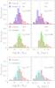Fig. 1

Distribution of stellar mass and effective radius for cluster and field elliptical galaxies. Upper panel − distribution of the stellar mass ℳ_∗ (left) and of the effective radius R_e (right) for the 56 cluster elliptical galaxies (red shaded histograms) and the 31 elliptical galaxies in the GOODS-South field (blue shaded histograms). The lower panels show the comparison with the field elliptical galaxies selected in the COSMOS area (green histograms). The colored solid line marks the median values of the distributions (see text). The dotted line marks the reference values log ℳ_∗ = 11.1 M_⊙ and R_e = 4 kpc above which the distributions are significantly different. Lower panel − same as in the upper panel but in this case the distributions of the cluster ellipticals are compared with those of the elliptical galaxies selected from CANDELS (cyan histograms; see Sect. 2).

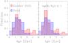Fig. 2

Age distribution of cluster and field ellipticals. Left − the distribution of the age of the stellar population of field elliptical galaxies (blue shaded histogram) is compared with the age distribution of all the cluster ellipticals (red shaded histogram).The colored solid lines mark the median values of the distributions (see text). Right − same as left panel but in this case the comparison is made by considering field and cluster ellipticals in the same mass range, that is, by excluding cluster galaxies with masses larger than log (ℳ_∗) = 11.1 M_⊙.

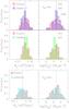Fig. 3

Distribution of mass-normalized radius and stellar mass density for cluster and field elliptical galaxies. Upper panel − distributions of the mass normalized radius (left) and of the effective stellar mass density Σ_{R_e} (right) for cluster (red histograms) and field elliptical galaxies in the GOODS-South field (blue histograms) and in the COSMOS area (green histograms). The effective radius R_e is normalized to the stellar mass $m_{*}^{0.5}$ $\hbox{$m_*^{0.5}$}$ where m_∗ = ℳ_∗/ 10¹¹M_⊙.Colored solid lines mark the median values of the distributions. The black dotted line marks the median value Σ_{R_e} = 2500 M_⊙ pc^-2 of the elliptical galaxies in cluster and in the GOODS-S field.Lower panel − same as in the upper panel but the comparison is made with the field elliptical galaxies selected in the CANDELS area (cyan histograms).

4.1. The population of elliptical galaxies and their dependence on the environment

Before comparing field and cluster samples, we verified that no significant cluster-to-cluster variation in the distributions of ages, effective radii, Sérsic index, and stellar masses were present. However, we note that, as can be seen from Table B.1, the fraction of galaxies with masses log(M_∗/M_⊙) > 11 in cluster XMM J2235, the one at highest redshit, is higher than in the other two clusters, even if this difference is not statistically significant. The absence of significant cluster-to-cluster variations is reflected in the agreement among the Kormendy relations (see Sect. 5).

In Fig. 1 the distributions of the stellar mass and of the effective radius of cluster galaxies are compared with those of field galaxies. The distributions show that elliptical galaxies in cluster reach higher stellar masses and larger radii than field ellipticals. Indeed, there is a lack of massive (ℳ_∗ > 2 × 10¹¹M_⊙ and large (R_e > 4−5 kpc) galaxies in the GOODS-S field at z ~ 1.3 with respect to the cluster environment at the same redshift (upper panel of Fig. 1), in agreement with what was found by Raichoor et al. (2011) at this redshift. This lack is statistically significant at more than 3σ as shown by the Kolmogorov-Smirnov (KS) test that provides a probability P_KS ≃ 0.004 that the observed distributions of stellar mass are extracted from the same parent population and a probability P_KS ≃ 0.04 (~2σ) for the distributions of the effective radius. Only 6% of the elliptical galaxies in the field are larger than R_e > 4 kpc while they are 21% in cluster. A consequence of this is that the median effective radius R_e is slightly larger in cluster (2.1 kpc) than in the field (1.5 kpc). The smaller number of large galaxies (>4−5 kpc) in the field is due to the lack of galaxies with mass higher than ~2 × 10¹¹M_⊙. The median stellar mass is larger in the cluster sample (6 × 10¹⁰M_⊙) than in the field (3.5 × 10¹⁰M_⊙) and while 21% of elliptical galaxies in cluster have masses ℳ_∗ > 1.2 × 10¹¹M_⊙, there are no galaxies exceeding this mass in the field.

These differences can be better assessed by comparing the two-dimensional distributions [R_e,ℳ_∗] of galaxies using the generalized KS test. Once compared in the mass range ℳ_∗ < 2 × 10¹¹M_⊙, cluster and field galaxies follow the same [R_e,ℳ_∗] distribution (P_{2 dKS} = 0.16) with the same median effective radius (1.7 kpc), while considering the whole mass range they differ at ~3σ (P_{2 dKS} = 0.01). This confirms that the two distributions differ because of the lack (excess) of massive and large galaxies in the field (in cluster). Contrary to that found by Papovich et al. (2012) at z ~ 1.6, we do not find a lack of small galaxies (R_e < 1 kpc) in cluster with respect to the field.

The lack of large and massive galaxies in the field at z ~ 1.3 is not a peculiarity of the GOODS-South region but is an actual property of the field environment, as confirmed by the comparison with the COSMOS and the CANDELS samples shown in the middle and in the lowest panels of Fig. 1 respectively. We note that the effective radii for galaxies in the COSMOS sample are given for values larger than ~0.17 arcsec (see Scarlata et al. 2007) that, at z ≃ 1.2, corresponds to ~1.3 kpc. Hence, to compare the distributions of R_e and of the quantities involving R_e (normalized effective radius and mass density) with the COSMOS sample, in the cluster sample we selected only galaxies with R_e> 1.3 kpc.

The lack of galaxies with mass higher than 2−3 × 10¹¹M_⊙ is significant both in the COSMOS area (~2σ significance, P_KS ≃ 0.05) and in the CANDELS fields (>5σ, P_KS< 10^-5). Analogously, elliptical galaxies with effective radius larger than 4−5 kpc are extremely rare at high significance level both in the COSMOS area (~3σ, P_KS ≃ 0.006) and in the CANDELS fields (>3σ, P_KS ≃ 0.003) with respect to the cluster environment.

The comparison of the two-dimensional distributions [R_e,ℳ_∗] confirms that the COSMOS and CANDELS samples differ (P_{2 dKS} = 0.02 and P_{2 dKS} = 2 × 10^-4 respectively) from the cluster sample for the high-mass galaxies, since they do not differ (P_{2 dKS} = 0.12 and P_{2 dKS} = 0.04) when only galaxies with ℳ_∗< 2 × 10¹¹M_⊙ are considered. A lack of massive galaxies in the field with respect to the cluster environment is not surprising given the known correlation between halo mass and stellar mass of the galaxies populating it (e.g., Lin et al. 2004; Beutler et al. 2013; Shankar et al. 2014a). For instance, Huertas-Company et al. (2013b) show that galaxies more massive than 10¹¹M_⊙ are two to three times more frequent in halos with masses of 10¹⁴M_⊙ than in halos one order of magnitude less massive. This may be due to the higher frequency of merging expected in higher density regions. Hence, it is expected that the field environment is less rich in high-mass and, consequently, large galaxies than the cluster environment, as seen also in the local Universe. In practice, some kind of environmental dependence in the population of (elliptical) galaxies in the two environments is expected.

In Fig. 2 the distributions of the mean age of the stellar population derived from the SED fitting are shown for cluster and field (GOODS-S) elliptical galaxies. It is well known that this age does not represent the age of the bulk of the stars, that is the formation redshift z_form, but rather the age of the stars producing the dominant light (e.g., Greggio & Renzini 2011). Hence, only old ages, compared to the age of the universe at the redshift of the galaxy, are indicative of or coincident with the formation redshift z_form while, in the other cases, they may be indicative of the last burst of star formation. Our goal is not to determine the age of the bulk of the stars in elliptical galaxies at z ~ 1.3 but, rather, to assess whether the stellar populations show differences correlated with the environment where the galaxies reside. Hence, this kind of luminosity-weighted age is suited to this purpose.

In the left panel of Fig. 2, the distributions of the two entire samples are compared. It is well known that a correlation between age and stellar mass exists: the larger the mass, the older the age. Hence, in the right panel, to delete the effect of the tail at high masses of cluster galaxies, we compare the distributions of galaxies selected in the same stellar mass range log ℳ_∗< 11.1 M_⊙. The median age of galaxies in the field is med(Age)_f ≃ 1.4 Gyr, slightly lower than in cluster (med(Age)_c ≃ 1.7 Gyr). Figure 2 shows that the oldest elliptical galaxies at z ~ 1.3 are in cluster and that there is a fraction of galaxies with old ages, older than ~3.5−4 Gyr (z_form> 5), not present in the field. As shown in the right panel of Fig. 2, this excess of old galaxies in cluster remains, even when the two samples are compared in the same mass range. Thus, it seems that there is a lack of elliptical galaxies in the field which are as old as the oldest elliptical galaxies in cluster. However, this lack is not statistically significant (P_KS ≃ 0.09).

The above comparisons show that the population of elliptical galaxies in cluster at z ~ 1.3 differs from the one in the field. There is a significant lack of massive and consequently large elliptical galaxies in the field with respect to the cluster environment, suggesting that the assembly of massive (ℳ_∗> 2−3 × 10¹¹M_⊙) and large (R_e> 4−5 kpc) elliptical galaxies at z ~ 1.3 is a prerogative of the cluster environment. Moreover, we find hints of the fact that the oldest elliptical galaxies at this redshift are in cluster, in agreement with what has been derived from the study of the elliptical galaxies in the local Universe (e.g., Thomas et al. 2005, 2010). These results suggest that either the assembly of massive galaxies takes place earlier or it is more efficient and faster in cluster than in the field (see also Menci et al. 2008; Rettura et al. 2010, 2011).

4.2. Structural properties of elliptical galaxies in cluster and in the field

In Fig. 3 the distributions of the mass-normalized radius $R_{e} / m_{*}^{a}$ $\hbox{$R_{\rm e}/m_*^a$}$ and of the mass surface density Σ_{R_e} of cluster galaxies are compared with those of field galaxies. Following Newman et al. (2012) and Cimatti et al. (2012; see also Huertas-Company et al. 2013a; Delaye et al. 2014; Allen et al. 2015), we defined the mass-normalized radius as $R_{e} / m_{*}^{a}$ $\hbox{$R_{\rm e}/m_*^a$}$ where m_∗ is the stellar mass of the galaxy in units of 10¹¹M_⊙, that is, m_∗ = ℳ_∗/ 10¹¹ [ M_⊙], and a = 0.5 is the best fitting slope of the size-mass relation of our samples of elliptical galaxies (see Sect. 6). The mass-normalized radius thus defined removes the dependence of the radius from the mass allowing the comparison of the size distributions of galaxies also in the case of different mass distributions. This allows us to determine whether cluster galaxies tend to be smaller or larger, denser or less dense than field galaxies independently of their mass. It is worth noticing that this is equivalent to comparing the effective stellar mass surface density of galaxies, perhaps a more meaningful quantity, defined as $Σ_{R_{e}} = ℳ_{*} / 2 π R_{e}^{2}$ $\hbox{$\Sigma_{R_{\rm e}}=\mathcal{M}_*/2\pi R_{\rm e}^2$}$ , being the mass normalized radius defined above the inverse of the square-root of Σ_{R_e}.

The distributions of the normalized effective radius of the cluster and field elliptical galaxies shown in Fig. 3, belong to the same parent population (P_KS ≥ 0.6). The median value is med( $R_{e} / m_{*}^{0.5}) = 2.7 \pm 0.2$ $\hbox{$R_{\rm e}/m_*^{0.5})=2.7\pm0.2$}$ kpc both in cluster and in the field (GOODS-S, COSMOS and CANDELS). The same result, that there is no difference in the compactness (in the size at fixed stellar mass) of galaxies in cluster and in the field, is provided by comparing the mass surface density distributions (right panels). We note that the median value of the stellar mass surface density is Σ_{R_e} ~ 2500 M_⊙ pc^-2 both for cluster and for field galaxies; that is, ~50% of galaxies are denser than this value both in cluster and in the field. The distributions and the above results remain unchanged both considering the samples in the same mass range (log ℳ_∗< 11.1 M_⊙) or in the whole mass range. Hence, cluster and field ellipticals do not show different structural properties.

At redshift similar to our study, Delaye et al. (2014) find that at 1.1 <z< 1.6 field galaxies in the mass range 3 × 10¹⁰−10¹¹M_⊙ are 10−30% smaller than cluster galaxies. However, the authors themselves notice that the apparent greater compactness of field galaxies may be due to the different wavelengths at which their effective radii were estimated. In particular, they used near-IR (optical rest-frame) size from CANDELS for field galaxies while using optical (U/B rest-frame, as in our study) size from ACS observations for cluster galaxies. The apparent size of galaxies can be different at different wavelengths (see, e.g., La Barbera et al. 2010) and, at z> 1, galaxies seen in the F160W filter appear 10−20% smaller than in the F850LP filter (e.g., Cassata et al. 2011; Gargiulo et al. 2012, but see also Appendix A.2]). Therefore, the apparent smaller size of field galaxies they found could be due to this effect. Supporting this hypothesis, we note that the median value of the mass normalized radius we measured in the ACS-F850LP filter both for cluster and field ellipticals, perfectly agrees with the one they derive for cluster galaxies (~2.8 kpc for a = 0.57) on the ACS images.

Raichoor et al. (2012) find that the population of smaller size elliptical galaxies at z ~ 1.3 is more numerous in denser environments (groups and clusters) than in the field environment, even if galaxies do not show different structures at fixed mass. In contrast, Papovich et al. (2012) find that, at fixed stellar mass, field galaxies at z ~ 1.6 are smaller, hence denser or more compact, than cluster galaxies. In line with our results, Newman et al. (2014; see also Rettura et al. 2010) find no significant difference between the size of field and cluster galaxies at z ~ 1.8 in the same mass range. Analogously, Allen et al. (2015) find no significant differences between the mass normalized radius of field and cluster quiescent galaxies at z ~ 2, for which they estimate a mean mass normalized semi-major axis a_{1 / 2,maj} ~ 2.0 kpc in the F160W filter. Allen et al. (2015) normalized the mass using 5 × 10¹⁰M_⊙ and the radius using a = 0.76. By scaling our effective radius according to these values, we obtain med( $R_{e} / m_{*}^{0.76}$ $\hbox{$R_{\rm e}/m_*^{0.76}$}$ )≃ 1.9 kpc. Assuming a mean axis ratio b/a = 0.7 (see Tables B.1 and B.2), that is a factor (b/a)^{− 1 / 2} ≃ 1.2 and a correction of 10% for the longer wavelength, our median radius translates into a median semi-major axis of ~2.1 kpc in the F160W filter, in agreement with the semi-major axis estimated by Allen et al. (2015) at z ~ 2.

At lower redshift than our study, Huertas-Company et al. (2013a) find no significant differences in the structural properties of field and cluster galaxies up to z ~ 1. Kelkar et al. (2015) find no significant difference in the size distribution of cluster and field galaxies at 0.4 < z < 0.8 both for a given morphology and for a given B−V color, ruling out average size differences larger than 10−20%. Shankar et al. (2014b) studied the dependence of the median sizes of central galaxies on host halo mass using a sample of galaxies at z < 0.3 extracted from the Sloan Digital Sky Survey (SDSS). They found no difference between the structural properties of early-type galaxies in different environments, at fixed stellar mass.

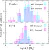Fig. 4

Stellar mass distribution of compact and normal galaxies in field and cluster environment. Upper panel − the distribution of the stellar mass of normal elliptical galaxies (magenta histogram) in cluster is compared to the one of compact galaxies (cyan histogram) defined according to the criterion log $(ℳ_{*} / R_{e}^{1.5}) > 10.3$ $\hbox{$(\mathcal{M}_*/R_{\rm e}^{1.5})>10.3$}$ . Lower panel − same as for the upper panel but for field elliptical galaxies.

We also considered the definition of a compact/dense galaxy based on the criterion log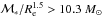 $ℳ_{*} / R_{e}^{1.5} > 10.3 M_{⊙}$ $\hbox{$\,\mathcal{M}_*/R_{\rm e}^{1.5}>10.3~M_\odot$}$ kpc^-1.5 (e.g., Barro et al. 2013; Poggianti et al. 2013b; Damjanov et al. 2015). Figure 4 shows the stellar mass distributions of cluster and field elliptical galaxies classified as compact/dense and normal according to this criterion. The fraction of compact galaxies in the field (39(± 11)%) is slightly lower than in cluster (48(± 9)%), even if this difference is not statistically significant. Hence we find that also the fraction of compact galaxies thus defined is similar in the two different environments, confirming the previous results.

We have shown that at fixed stellar mass, elliptical galaxies in cluster and in the field at 1.2 < z < 1.4 are characterized by the same structural parameters. Elliptical galaxies in the field have a similar density to those in cluster; their stellar mass density and their structural parameters are not dependent on the environment where they reside. What we see is that ultramassive, (ℳ_∗> 2−3 × 10¹¹M_⊙) large (R_e> 4−5 kpc) early-type galaxies at z ~ 1.3 are more abundant in the cluster environment than in the field environment. We could suppose that in the field, the assembly of such massive early-type galaxies takes place over a longer time or that it starts later than in cluster, and that the lack of ultramassive elliptical galaxies in the field is filled up at lower redshift. However, this is not the case. Indeed, the number density of ultramassive dense elliptical galaxies in the field seems to be constant over the redshift range 0.2 < z < 1.5 (Gargiulo et al. 2016). This suggests that both the populations of high-mass elliptical galaxies, in cluster and in the field, are mostly formed at that redshift. This could be explained if the assembly of massive galaxies is more efficient in cluster than in the field. Clear evidences in favor of this has still not emerged from observations, however, some analyses point toward a faster star formation in cluster than in the field (e.g., Rettura et al. 2011; Guglielmo et al. 2015) and others show that the stellar mass distribution in the central parts of the mass distribution in clusters are already in place at z ~ 1 (van der Burg et al. 2015; see also Vulcani et al. 2016). Irrespective of this, the fact that cluster and field elliptical galaxies are characterized by the same structural parameters suggests that the formation processes acting in the two environments are the same.

5. The Kormendy relation of cluster and field elliptical galaxies at z = 1.3

Elliptical galaxies both in field and in clusters follow the scaling relation 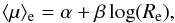$⟨ μ ⟩_{e} = α + β \log (R_{e}),$ $\begin{equation} \langle\mu\rangle_{\rm e} = \alpha + \beta \log(R_{\rm e}), \label{kr} \end{equation}$ (2)(Kormendy 1977, KR hereafter), a relation between the logarithm of the effective radius R_e [kpc] and the mean surface brightness ⟨ μ ⟩ _e within R_e. The slope parameter β ~ 3 in the B-band is found not to vary out to z ~ 1 (e.g., Hamabe & Kormendy 1987; Schade et al. 1996; Ziegler et al. 1999; La Barbera et al. 2003; Reda et al. 2004; di Serego Alighieri et al. 2005; Saracco et al. 2009; 2014) as also shown from the studies of the fundamental plane of galaxies (e.g., Graham et al. 2006; D’Onofrio et al. 2008; Gargiulo et al. 2009; Saglia et al. 2010; Jørgensen et al. 2014; Zahid et al. 2016). Possibly, a slightly steeper slope is found at higher stellar masses (ℳ > 3−4 × 10¹¹M_⊙) typically for brightest cluster galaxies (BCGs; e.g., Bai et al. 2014; Bildfell et al. 2008; von der Linden et al. 2007). The different slope could suggest a disparity in the M/L or a break in the homology at these masses (e.g., von der Linden et al. 2007). Actually, at these large stellar masses, galaxies seem to deviate from the scaling relations defined by galaxies with lower masses, suggesting that the mass accretion at such large masses may take place according to different mechanisms (e.g., Bernardi et al. 2011, 2014). Contrary to the slope, the zero point α of the KR is found to vary with the redshift of the galaxies according to the expected luminosity evolution.

In this section, we derive and compare the Kormendy relation of cluster and field elliptical galaxies at z ~ 1.3 in order to asses whether the environment plays a role in shaping this relation. We consider here the B-band rest-frame since morphological parameters have been derived in the F850LP filter sampling λ_rest ≃ 4000 Å at z ~ 1.3. For each galaxy we derived the mean effective surface brightness $⟨ μ ⟩_{e}^{B} = M_{B} (z) + 2.5 \log (R_{e}^{2}) + 38.57,$ $\begin{equation} \langle\mu\rangle_{\rm e}^B =M_B(z)+2.5{\rm log}(R_{\rm e}^2)+38.57, \label{murest} \end{equation}$ (3)where M_B(z) is the absolute magnitude of the galaxy in the rest-frame B-band at redshift z, and R_e is in [kpc], after correcting for the cosmological dimming term 10log(1 + z). The surface brightnesses thus obtained are reported in Table 1.

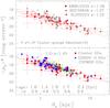Fig. 5

Kormendy relation in the rest-frame B-band for cluster and field elliptical galaxies at z ≃ 1.3. Upper panel− the B-band surface brightness of the 17 galaxies in the cluster XMMU2235 at z ~ 1.39 (dark red filled squares), of the 16 galaxies in the RDCS0848 at z ~ 1.27 (brick red filled circles), and of the 23 galaxies in the cluster XLSS0223 at z ~ 1.22 (red filled triangles) are plotted as a function of their effective radius R_e at the redshift of the clusters. The three colored lines are the best fitting Kormendy relations to the three clusters reported in Table 1. The open symbols are the sample of early-type galaxies in the Linx clusters and groups studied by Raichoor et al. (2012). Lower panel: the surface brightness of the 56 cluster galaxies (red filled circles), of the 31 field galaxies at 1.2 <z< 1.45 in the GOODS-South region (blue filled squares), and of the 178 galaxies at 1.0 <z< 1.2 in the COSMOS area (green filled triangles) are plotted as a function of their effective radius. The red solid line and the blue dashed line are the best fitting relations obtained for cluster and GOODS-S field galaxies respectively, and are reported in Table 1. At the bottom of the figure, the mean age ⟨ age ⟩ [Gyr] of galaxies in the different intervals of effective radius together with its dispersion (σ) is reported.

In the upper panels of Fig. 5, the rest-frame B-band surface brightness of the elliptical galaxies in the cluster XMM J2235 at z ≃ 1.39, RDCS0848 at z ≃ 1.27, and in the cluster XLSS0223 at z ≃ 1.22 is plotted as a function of their effective radius R_e. The solid colored lines are the best fitting Kormendy relations we obtained using the least square fit for the three clusters and are summarized in Table 1.

Table 1

Kormendy relation of cluster and field ellipticals at z ~ 1.3.

The relations found are in agreement between them and they are described by the same slope β ≃ 3.1 (see Table 1). The brightening by about 0.4 mag of the zeropoint α of the KR of the XMMU2235 cluster, reflects the significantly higher redshift, in terms of luminosity evolution, of this cluster with respect to the other two. Indeed, by computing for each galaxy of the XMMU2235 cluster the luminosity evolution since z = 1.39, we found that, on average, galaxies would get fainter by 0.35( ± 0.1) mag at z = 1.25 (Δt ~ 0.4 Gyr), in agreement with the different zeropoint. The distribution of the galaxies in the [μ_e, R_e] plane and the relevant best fitting relations do not show significant differences among the populations of elliptical galaxies (EGs) in these three clusters. So, we have defined the KR for cluster ellipticals at z ~ 1.3 considering the whole sample of 56 cluster galaxies. The resulting best fitting KR for the whole sample is $⟨ μ ⟩_{e}^{B} = 17.7 (\pm 0.1) + 3.0 (\pm 0.2) \log (R_{e}) Cluster z \in [1.2 - 1.4],$ $\begin{equation} \langle\mu\rangle_{\rm e}^B=17.7(\pm0.1)+3.0(\pm0.2){\rm log}(R_{\rm e})\hskip 0.3truecm {\rm Cluster}\\\ z\in[1.2{-}1.4], \label{krmean} \end{equation}$ (4)in good agreement with that found by Jørgensen et al. (2014) and Raichoor et al. (2012) at the same redshift (see Appendix A for the orthogonal fit). The slope of the KR we find at z ~ 1.3 agrees also with the slope found at intermediate redshift (Saglia et al. 2010; Jørgensen & Chiboucas 2013; Zahid et al. 2016) and in the local Universe (e.g., Jørgensen et al. 1995; D’Onofrio et al. 2008; Gargiulo et al. 2009; La Barbera et al. 2010).

In the lower panel of Fig. 5, the surface brightness of the 31 field elliptical galaxies in the redshift range 1.2 <z< 1.45 in the GOODS-S region is plotted as a function of their effective radius and superimposed onto the sample of cluster galaxies at the same redshift. The resulting best fitting KR to field elliptical galaxies is $⟨ μ ⟩_{e}^{B} = 17.5 (\pm 0.2) + 3.3 (\pm 0.3) \log (R_{e}) Field z \in [1.2 - 1.4] .$ $\begin{equation} \langle\mu\rangle_{\rm e}^B=17.5(\pm0.2)+3.3(\pm0.3){\rm log}(R_{\rm e})\hskip 0.3truecm {\rm Field}\\\ z\in[1.2{-}1.4]. \label{krfield} \end{equation}$ (5)The slope is slightly steeper than the one for cluster galaxies even if the difference is not statistically significant. We verified that this small difference is due to the massive and large (R_e> 4−5 kpc) cluster galaxies not present in the field (see previous section), which tend to slightly flatten the relation. For comparison, we also plotted the 178 EGs selected in the COSMOS area at 1.0 <z< 1.2 with measured effective radius. This sample is highly incomplete for radii <1.3 kpc since measurements of radii are available in the catalog for values larger than ~0.17 arcsec (see Sect. 2.2).

The distribution of the galaxies in the [μ_e, R_e] plane and the best fitting relations found show that cluster and field elliptical galaxies at ~1.3 follow the same size-surface brightness relation. We find no evidence statistically significant of a dependence of the KR on the environment at z ~ 1.3, in agreement with what has been previously found by other authors (Rettura et al. 2010; Raichoor et al. 2012) at similar redshift. Analogously, we find that the zeropoint of the KR of early-type galaxies at this redshift is about two magnitudes brighter than at z = 0, as also found by Holden et al. (2005), Rettura et al. (2010), Raichoor et al. (2012), and Saracco et al. (2014) on samples of cluster and group galaxies at similar redshift.

At the bottom of Fig. 5, we report the mean age of galaxies in different intervals of effective radius. As can be seen, there is a variation of the age of galaxies along the Kormendy relation, as previously noticed by Raichoor et al. (2012): the age tends to increase going toward larger and lower surface brightness galaxies. This small age gradient is related to the age-mass relation in which higher mass galaxies (larger and usually with lower surface brightness) are older than lower mass ones.

6. The size-mass relation

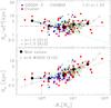Fig. 6

Effective radius-stellar mass relation for elliptical galaxies. Upper panel − the mass normalized radius $R_{e} / m_{*}^{0.5}$ $\hbox{$R_{\rm e}/m_*^{0.5}$}$ is plotted as a function of the stellar mass ℳ_∗. The filled symbols are the cluster ellipticals of our sample (red circles), the field ellipticals we selected at 1.2 <z< 1.45 in the GOODS-S field (blue squares), and the ellipticals at 1.0 <z< 1.2 in the COSMOS field (green crosses). Open symbols are data taken from Raichoor et al. (2012; R12, stars), from Delaye et al. (2014; D14, triangles), and from Valentinuzzi et al. (2010 V10, circles; see also Poggianti et al. 2013a). The green short-dashed line is $y = 1.3 [kpc] / m_{*}^{0.5} + c$ $\hbox{$y=1.3[{\rm kpc}]/m_*^{0.5}+c$}$ , the line below which there are no measured effective radii in the COSMOS catalog (Sargent et al. 2007). We report errorbars only in the lower panel just for clarity in the plot. Lower panel − the effective radius R_e is plotted versus the stellar mass. Symbols are as in the upper panel. The big black filled triangles are the median values of our sample of cluster and field ellipticals at z ~ 1.3. The long-dashed line is the best fitting relation $R_{e} \propto ℳ_{*}^{0.5}$ $\hbox{$R_{\rm e}\propto\mathcal{M}_*^{0.5}$}$ over the whole mass range.

Figure 6 shows the size-mass relation for cluster and field elliptical galaxies at z ~ 1.3 . In the upper panel, we show the mass normalized effective radius $R_{e} / m_{*}^{0.5}$ $\hbox{$R_{\rm e}/m_*^{0.5}$}$ (see Sect. 4) as a function of stellar mass, while in the lower panel we show the effective radius versus the mass. Superimposed onto our data, we plot for comparison the early-type galaxies, in groups and in cluster at z ~ 1.27, of the sample of Raichoor et al. (2011, 2012, hereafter R12). They derived stellar masses adopting the Salpeter IMF. Thus, we scaled their masses by a factor 1.7 to match them to the Chabrier IMF, according to the recipe of Longhetti & Saracco (2009) and to that found for elliptical galaxies at this redshift (Saracco et al. 2014; Tamburri et al. 2014). Besides this sample, we also plotted the cluster early-type galaxies belonging to the sample of Delaye et al. (2014, hereafter D14) in the redshift range 1.22 <z< 1.4 that have stellar masses based on Chabrier IMF, as for our data. These two samples cover almost the same mass range as that covered by our data, extending down to 2 × 10¹⁰M_⊙ at low masses and up to 2 × 10¹¹M_⊙ at high masses. The effective radii for both the samples have been derived on the ACS-F850LP images, as for our data. As can be seen, the agreement among the different samples is very good.

In the mass range ~10¹⁰−10¹¹M_⊙, well covered by field and cluster ellipticals, galaxies in the two environments do not show differences in the size-mass plane. The median effective radius of cluster ellipticals is 1.4 ± 0.7 kpc for ℳ_∗ ∈ [10¹⁰−5 × 10¹⁰] M_⊙ and 2.1 ± 0.6 kpc for ℳ_∗ ∈ [5 × 10¹⁰−10¹¹] M_⊙, to be compared with 1.3 ± 0.4 kpc and 2.0 ± 0.8 kpc for field ellipticals in the same mass ranges (the quoted errors are the median absolute deviation). Similar results, that there is no evidence of a dependence of the size-mass relation on the environment, are found by Rettura et al. (2010), Raichoor et al. (2012), Newman et al. (2014), and Allen et al. (2015) at redshift comparable or higher than ours, and by Kelkar et al. (2015) and Huertas-Company et al. (2013a) at intermediate redshift (0.4 <z< 1). To our knowledge, at intermediate and high redshift, Cooper et al. (2012), Lani et al. (2013), and Strazzullo et al. (2013) find a correlation between the size of massive quiescent galaxies and the environment where they reside: galaxies in denser environments are much larger (less dense) then galaxies in low density environments. However, in these latter works, the selection of galaxies is based on the Sersic index and/or on UVJ colors instead of on morphology, making a reliable comparison difficult. Selections based on colors or Sersic index provide samples with a different mix of morphological types (e.g., Mei et al. 2012; Tamburri et al. 2014). It has been clearly shown that the size of galaxies at fixed mass is a strong function of morphology (e.g., Mei et al. 2012; Bernardi et al. 2014). The different fractions of morphological types in the different environments that these selection criteria provide, could give rise to different results (see also the discussion in Newman et al. 2014).

In the local Universe, where the statistic is higher than at higher redshift, the results seem to confirm the absence of strong dependence on the environment. Poggianti et al. (2013a), using the cluster galaxies in the Wide-field Nearby Galaxy-clusters Survey (WINGS, Fasano et al. 2006; Valentinuzzi et al. 2010) and the field galaxies of the Padova-Millennium Galaxy and Group Catalog (PM2GC, Calvi et al. 2011), find that the mass-size relation of cluster galaxies lies slightly (~1σ) below the relation for field galaxies. They note that, for a given mass, the fraction of smaller (i.e., denser) galaxies in cluster is slightly higher than the fraction in the field. Perhaps, this reflects the larger fraction of lenticular galaxies present in the cluster sample than in the field sample, since lenticular galaxies tend to be smaller than ellipticals at fixed stellar mass (e.g., Maltby et al. 2010; Bernardi et al. 2014). Huertas-Company et al. (2013b) using the Sloan Digital Sky Survey data (SDSS, DR7, Abazajian et al. 2009) find no differences between the size-mass of early-type galaxies in the two environments, a result emerging also from the analysis of Shankar et al. (2014b) and, previously, from the analysis of Maltby et al. (2010) and Rettura et al. (2010). Thus, it seems that if differences in the size-mass relation of elliptical galaxies depending on the environment are present, they have to be small and due to differences in the population of galaxies rather than in the structural properties of galaxies at fixed type and mass.

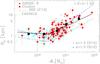Fig. 7

Effective radius-stellar mass relation for elliptical galaxies. Filled symbols are field (squares) and cluster (circles) ellipticals of our sample. Empty symbols are as Fig. 6. The thick solid lines are the best fitting relations obtained with the least square fit for values lower and higher than ℳ_∗ = 2.5 × 10¹⁰M_⊙, $R_{e} = 26 \times ℳ_{*}^{- 0.13 \pm 0.2}$ $\hbox{$R_{\rm e}=26\times\mathcal{M}_*^{-0.13\,\pm\,0.2}$}$ , and $R_{e} = 2.77 \times 10^{-7} ℳ_{*}^{0.64 \pm 0.09}$ $\hbox{$R_{\rm e}=2.77\times10^{-7}\mathcal{M}_*^{0.64\pm0.09}$}$ respectively. The blue dashed line is the best fitting relations obtained in the two mass ranges using the orthogonal fit (see Appendix A), $R_{e} \propto ℳ_{*}^{- 0.3 \pm 0.2}$ $\hbox{$R_{\rm e}\propto\mathcal{M}_*^{-0.3\,\pm\,0.2}$}$ and $R_{e} \propto ℳ_{*}^{1.0 \pm 0.1}$ $\hbox{$R_{\rm e}\propto\mathcal{M}_*^{1.0\pm0.1}$}$ respectively. The gray dot-dashed line is the relation R_e = 0.53(ℳ_∗/ 3 × 10¹⁰)^-0.2(0.5 + 0.5(ℳ_∗/ 3 × 10¹⁰)^0.8)^0.119 defining the Zone of Exclusion (ZOE) as obtained by Cappellari et al. (2013a) and scaled by a factor $⟨ R_{e} / R_{e}^{maj} ⟩ = 0.76$ $\hbox{$ \langle R_{\rm e}/R_{\rm e}^{\rm maj} \rangle\,=\,0.76$}$ (see text). Open symbols represent the samples of Raichoor et al. (2012; stars, R12) and of Delaye et al. (2014; triangles, D14).Cyan crosses are elliptical galaxies selected from CANDELS.

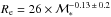
Even if the following issue is not the focus of the present paper, we believe that it deserves to be at least mentioned. By fitting the size-mass relation to the whole sample of cluster and field elliptical galaxies over the whole mass range with a single power law of the form $R_{e} = b ℳ_{*}^{a}$ $\hbox{$R_{\rm e}=b\mathcal{M}_*^a$}$ , we find $\log (R_{e}) = 0.5 (\pm 0.06) \log ℳ_{*} - 5.0 (\pm 0.7),$ $\begin{equation} {\rm log}(R_{\rm e})=0.5(\pm0.06){\rm log}\,\mathcal{M}_*-5.0(\pm0.7), \label{eq_size} \end{equation}$ (6)using the least square method (see Appendix A for the orthogonal fit). Figure 6 shows clearly that a single power law does not provide a good fit to the data over the whole mass range considered and that the relation tends to be curved consistently with other relations (see, e.g., Graham 2013, for a review). In particular, the observed median size relation deviates significantly from a single power law and changes the slope at a transition mass m_t ≃ 2−3 × 10¹⁰M_⊙: at lower masses, the relation tends to flatten, while at masses larger than this the relation tends to steepen. The changing of some relationships in correspondence with this value of mass scale has been previously noted in the local Universe (e.g., Kauffmann et al. 2003; Shankar et al. 2006). The changing slope of the size-mass relation and the flattening at low masses in our data at z ~ 1.3 is better visible in Fig. 7. This feature is visible in all the samples that extend down to at least 10¹⁰M_⊙ (e.g., Valentinuzzi et al. 2010; Maltby et al. 2010; Cappellari et al. 2013a; Lani et al. 2013; Kelkar et al. 2015) and it has been previously noticed in the local samples of early type galaxies and discussed by Bernardi et al. (2011, 2014). 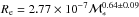Considering a broken power law and fixing the transition mass at m_t ~ 2.5 × 10¹⁰M_⊙, we find that the effective radius of elliptical galaxies scales with stellar mass as $R_{e} = 26 \times ℳ_{*}^{- 0.13 \pm 0.2} for ℳ_{*} < m t$ $\begin{equation} R_{\rm e}=26\times\mathcal{M}_*^{-0.13\pm0.2}\\\\\\\\\\\\ {\rm for} \\\ \mathcal{M}_*<m_{\rm t} \end{equation}$ (7)and $R_{e} = 2.77 \times 10^{-7} ℳ_{*}^{0.64 \pm 0.09} for ℳ_{*} > m_{t},$ $\begin{equation} R_{\rm e}=2.77\times10^{-7}\mathcal{M}_*^{0.64\pm0.09} \\\\\\\ {\rm for} \\\ \mathcal{M}_*>m_{\rm t}, \end{equation}$ (8)in the case of the least square fit (see Appendix A for orthogonal fit). Hence, the effective radius remains nearly constant at ~1 kpc and the relation is nearly flat for stellar masses lower than ~3 × 10¹⁰M_⊙, while it systematically increases at larger masses. It follows that, at masses <3 × 10¹⁰M_⊙, the stellar mass density Σ_{R_e} of galaxies increases rapidly with mass up to the transition mass where it reaches the maximum. Indeed, as can be seen from Fig. 8, the highest values of Σ_{R_e} are for galaxies with masses close to 3 × 10¹⁰M_⊙. At higher masses, the radius increases as $R_{e} \propto ℳ_{*}^{0.64}$ $\hbox{$R_{\rm e}\propto\mathcal{M}_*^{0.64}$}$ and the stellar mass density decreases. Given the similarity, this behavior has to be related to the zone of exclusion (ZOE) empirically defined by Bender et al. (1992) and by Burstein et al. (1997) for galaxies at small sizes and at large densities. This is shown in Fig. 7 where we also reproduce the best fitting ZOE relation obtained by Cappellari et al. (2013a) in the local Universe from the ATLAS^3D sample. They define the relation in their Eq. (4) by using the major axis $R_{e}^{maj}$ $\hbox{$R_{\rm e}^{\rm maj}$}$ instead of the effective radius. We derive R_e, by re-scaling the major axis $R_{e}^{maj}$ $\hbox{$R_{\rm e}^{\rm maj}$}$ of Eq. (4) of a factor $⟨ R_{e} / R_{e}^{maj} ⟩ = 0.76$ $\hbox{$ \langle R_{\rm e}/R_{\rm e}^{\rm maj} \rangle ~=~0.76$}$ , the mean value derived from the ATLAS^3D sample (Cappellari et al. 2013b). We do not further investigate here the meaning of the transition mass.

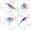Fig. 8

Stellar mass surface density versus effective radius and stellar mass. Upper panel − the effective stellar mass density within the effective radius $Σ_{R_{e}} = ℳ_{*} / 2 π R_{e}^{2}$ $\hbox{$\Sigma_{R_{\rm e}}=\mathcal{M}_*/2\pi R_{\rm e}^2$}$ , is plotted as a function of the effective radius R_e (left) and of the stellar mass ℳ_∗ (right). Blue filled squares are field ellipticals in the GOODS-S regions, green crosses are those in the COSMOS area, and red filled circles are cluster ellipticals. The black solid line is the best-fitting relation $Σ_{R_{e}} \propto R_{e}^{- 1.2 \pm 0.1}$ $\hbox{$\Sigma_{R_{\rm e}}\propto R_{\rm e}^{-1.2\pm0.1}$}$ (see Appendix A for the orthogonal fit). The green dashed line in the right panel shows the stellar mass density as a function of mass for a constant value of R_e = 1.3 kpc (marked on the left panel), corresponding to the limiting value ~0.17 arcsec adopted for the effective radius in the COSMOS catalog of Scarlata et al. (2007). The gray dot-dashed line marks the Zone of Exclusion (ZOE) as defined in Sect. 6.1. The open stars are the early-type galaxies selected by Raichoor et al. (2011; R11) in groups and clusters at z ~ 1.27. The open triangles are the cluster elliptical galaxies at 1.22 <z< 1.4 studied by Delaye et al. (2014; D14).The cyan crosses are the elliptical galaxies from CANDELS. Lower panel − the central stellar mass density calculated within 1 kpc radius (Σ_{1 kpc}) is plotted as a function of the effective radius (left) and of the stellar mass (right). Symbols are as in the upper panel. The solid black line is the best-fitting broken power law $Σ_{1 kpc} \propto ℳ_{*}^{(0.64 \pm 0.06)}$ $\hbox{$\Sigma_{1\,{\rm kpc}}\propto\mathcal{M}_*^{(0.64\pm0.06)}$}$ for ℳ_∗>m_t and $Σ_{1 kpc} \propto ℳ_{*}^{(1.07 \pm 0.1)}$ $\hbox{$\Sigma_{1\,{\rm kpc}}\propto\mathcal{M}_*^{(1.07\pm0.1)}$}$ for ℳ_∗<m_t, with m_t = 2.5 × 10¹⁰M_⊙. The gray dashed line is the relation found by Tacchella et al. (2016) with their model of mass growth and quenching, arbitrarily normalized.Errorbars are not shown to observe the agreement among the different samples and the relations defined by the data.

7. On the effective and the central stellar mass densities of elliptical galaxies

7.1. The effective stellar mass density

In the upper panels of Fig. 8, the effective stellar mass density $Σ_{R_{e}} = ℳ_{*} / 2 π R_{e}^{2}$ $\hbox{$\Sigma_{R_{\rm e}}=\mathcal{M}_*/2\pi R_{\rm e}^2$}$ of elliptical galaxies at z ~ 1.3 is shown as a function of their effective radius (left) and of their stellar mass (right). Superimposed onto our data, the samples of Raichoor et al. (2011, hereafter R11, 2012), of Delaye et al. (2014) andthe one selected from CANDELS are also shown.

The correlation between the effective mass density and the effective radius is a different way to represent the Kormendy relation being Σ_{R_e} related to ⟨ μ_e ⟩ = −2.5log ⟨ I_e ⟩ through the mass to light ratio of the galaxy. Actually, the definition of Σ_{R_e} here and commonly adopted does not take into account the presence of color gradients observed in most of the early-type galaxies at high redshift (e.g., Gargiulo et al. 2011, 2012; Guo et al. 2011; Chan et al. 2016; Ciocca et al., in prep.). Color gradients imply that the M/L is not radially constant and that, consequently, the stellar mass profile does not follow exactly the surface brightness profile. Hence, 50% of the stellar mass will not be contained within the half-light radius R_e, and the fraction of the stellar mass within R_e will be slightly but systematically different than 0.5. Indeed, the observed color gradients of elliptical galaxies at these redshift are systematically in one direction or null, both for field ellipticals (Gargiulo et al. 2011, 2012; Guo et al. 2011) and for cluster ellipticals (Ciocca et al., in prep.). Hence, this would reflect in a small offset of the relation along Σ_{R_e} and, since the variation can slightly differ from galaxy to galaxy, this would contribute to the observed scatter of the relation.

The correlation shown in Fig. 8 is best fitted by the relation $\log (Σ_{R_{e}}) = - 1.2 (\pm 0.1) \times \log (R_{e}) + 3.67 (\pm 0.05),$ $\begin{equation} {\rm log}(\Sigma_{R_{\rm e}})=-1.2(\pm0.1)\times {\rm log}(R_{\rm e})+3.67(\pm0.05), \end{equation}$ (9)where Σ_{R_e} [M_⊙ pc^-2] and R_e [kpc]. It is worth noting that the best fitting Kormendy relation obtained for the whole sample (see Table 1, ⟨All⟩) being −2.5log ⟨ I_e ⟩ ∝ 3.2 R_e, would imply a slope −1.28 of the Σ_{R_e}−R_e relation if the M/L was constant along the Kormendy relation. However, given the small age gradient (see Sect. 6), it follows that a variation of the M/L along the relation takes place, generating the small difference in the slope.

No significant difference is found by fitting field and cluster galaxies separately, as in the case of the Kormendy relation. Field and cluster galaxies follow the same Σ_{R_e}−R_e relation and occupy the same region of the plane, apart from the lack of massive and large galaxies in the field with respect to the cluster environment. The same slope is obtained by fitting the sample of Raichoor et al. (2011; b ≃ −1.3), while a slightly steeper slope (b ≃ −1.5) is found for the sample of Delaye et al. (2014). We note that the slope of this relation (~−1.2) seems to be constant over a wide redshift range: studying the mass fundamental plane of early type galaxies at z ~ 0, Hyde & Bernardi (2009) find a slope b ≃ −1.19; Zahid et al. (2016) find this slope for quiescent galaxies at z ~ 0.7 (see also Bezanson et al. 2015), while Bezanson et al. (2013) find that this slope well reproduces compact massive galaxies out to z ~ 2.

It is important to note that Fig. 8, besides showing that cluster and field elliptical galaxies occupy the same locus in the Σ_{R_e}−ℳ_∗ plane (upper right-hand panel), shows that Σ_Re is not correlated to the stellar mass of the galaxy. Galaxies with high or low effective stellar mass densities can be realized independently of their stellar mass, that is, dense/compact galaxies can be assembled in any mass regime independently of the environment in which they reside, cluster or field. Actually, the data show that not all the values of Σ_{R_e} can be realized for a given mass, according to the ZOE relation (see Fig. 6) that defines the locus that galaxies occupy in the [Σ_{R_e}−R_e,ℳ^∗] planes. As noted in the previous section, the highest values of effective stellar mass density are reached by galaxies with stellar mass close to the transition mass ~3 × 10¹⁰M_⊙ that, in our sample is Σ_{R_e} ~ 22 600 M_⊙ pc^-2 for a galaxy of mass ~3.5 × 10¹⁰M_⊙.

7.2. The central stellar mass density

In Fig. 8 (lower panels) the central stellar mass density Σ_{1 kpc} defined as the mass density within 1 kpc radius, is shown as a function of the effective radius (left) and of the stellar mass (right). Following Saracco et al. (2012), we derived the stellar mass interior to 1 kpc multiplying the luminosity within this fixed radius by the mass-to-light ratio of the galaxy 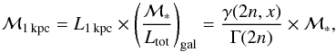$ℳ_{1 kpc} = L_{1 kpc} \times {(\frac{ℳ_{*}}{L_{tot}})}_{gal} = \frac{γ (2 n,x)}{Γ (2 n)} \times ℳ_{*},$ $\begin{equation} \mathcal{M}_{1\,{\rm kpc}}={L_{1\,{\rm kpc}}}\times\left ({\mathcal{M}_*\over L_{\rm tot}}\right )_{\rm gal} ={\gamma(2n,x)\over \Gamma(2n)}\times\mathcal{M}_*, \end{equation}$ (10)where 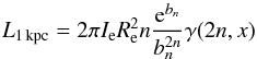$L_{1 kpc} = 2 π I_{e} R_{e}^{2} n \frac{e^{b_{n}}}{b_{n}^{2 n}} γ (2 n,x)$ $\begin{equation} L_{1\,{\rm kpc}}=2\pi I_{\rm e}R_{\rm e}^2 n {{\rm e}^{b_n}\over{b_n^{2n}}}\gamma(2n,x) \label{l1} \end{equation}$ (11)is the luminosity within the central region of 1 kpc, L_tot is the total luminosity obtained by replacing in Eq. (11) γ(2n,x) with the complete gamma function Γ(2n) (Ciotti 1991), and ℳ_∗ is the stellar mass of the galaxy obtained from the SED fitting. In Eq. (11), n is the Sérsic’s index, x = b_n(R₁/R_e)^{1 /n}, and γ(2n,x) is the incomplete gamma function. We assumed the analytic expression b_n = 1.9992n−0.3271 (Capaccioli & Corwin 1989) to approximate the value of b_n.

Figure 8 shows that the central stellar mass density Σ_{1 kpc} is tightly correlated with the stellar mass of galaxies, as already shown by Saracco et al. (2012), while it is independent of the effective radius, at the opposite of the effective mass density. The correlation is best fitted by the relation $\log (Σ_{1 kpc}) = 0.64 (\pm 0.06) \times \log ℳ_{*} - 3.2 (\pm 0.6),$ $\begin{equation} {\rm log}(\Sigma_{1\,{\rm kpc}})=0.64(\pm0.06)\times {\rm log}\,\mathcal{M}_*-3.2 (\pm0.6), \end{equation}$ (12)in good agreement with what was previously found for early-type galaxies both at 1 <z< 2 and in the local Universe (Saracco et al. 2012), for massive elliptical galaxies in cluster at z ~ 0.5 (Bai et al. 2014), but also for star forming galaxies at z ~ 2.2 (Tacchella et al. 2015) and in the local Universe (Fang et al. 2013). Also in this case, cluster and field ellipticals follow the same relation.

However, it can be seen that also the Σ_{1 kpc}-mass relation follows two different regimes, above and below the transition mass: at masses m_t< 2.5 × 10¹⁰M_⊙ the relation tends to steepen with $Σ_{1 kpc} \propto ℳ_{*}^{1.07 \pm 0.1}$ $\hbox{$\Sigma_{1\,{\rm kpc}}\propto\mathcal{M}_*^{1.07\pm0.1}$}$ . The transition mass defines a transition central mass density Σ_{1 kpc} ≃ 2−3 × 10³M_⊙ pc^-2. It is interesting to note that the presence of two different regimes and the slopes that we find agree with that found by Tacchella et al. (2016) in their simulations. They find a flattening of the Σ_{1 kpc}-mass relation when the galaxies reach masses ℳ_∗> 10^10.2M_⊙ (see their Fig. 8). The two different regimes they found should represent two different phases in the stellar mass growth of the galaxies.

We note that high-mass galaxies are centrally denser than lower mass ones but this is not true when the effective radius is considered. Indeed, as shown in Fig. 9 (see also Saracco et al. 2012), the correlation between the central and the effective stellar mass density is characterized by a very large scatter and, as shown by Fig. 8, the same value of effective mass density can be realized over a wide range of stellar mass, especially low density values. Hence, it is the galaxy central region which is strictly connected to the total stellar mass of the galaxy and, consequently, to its main mass growth. The tight linear relation between the central mass density and the stellar mass suggests a direct connection between the central regions and the earliest phases of formation during which most of the stellar mass is formed and assembled.

Contrary to the central density, the effective mass density and hence the regions at larger radii, are very weakly dependent on the mass suggesting that they are not good tracers of the growth of the bulk of the mass of the galaxy. The effective radius and hence the effective density, may have been strongly affected by episodes of relaxation, of inside-out quenching (Tacchella et al. 2016), and of minor mass accretion (minor mergers) that may have taken place after the growth of the bulk of the mass and before z ~ 1.3. This could explain the large scatter in the Σ_{1 kpc}−Σ_{R_e} relation. The scaling of the central mass density with mass suggests that the process of assembly and of shaping of the ellipticals is invariant with mass, at least in the mass range considered.

Figure 10 shows the central stellar mass density as a function of the stellar mass for field and cluster elliptical galaxies. Symbols have different colors according to the age resulting from the best fitting to their SED. The large symbols represent the median age of galaxies in four different mass bins. The figure shows that the higher the central mass density, the higher the mass, the older the stellar population. The correlation between central density and age is better shown in the left panel of the figure. The higher central mass density of high-mass galaxies reflects the higher normalization of their mass profile with respect to lower mass ones and, again, the close connection with the main episode of star formation. The older age may suggest that higher mass galaxies underwent less subsequent episodes of star formation at later times or that their massive burst takes place earlier than lower mass ones.

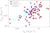Fig. 9

Central versus effective stellar mass density. The central stellar mass density calculated within 1 kpc radius (Σ_{1 kpc}) is plotted as a function of the effective stellar mass density (Σ_{R_e}). Blue filled squares are field ellipticals in the GOODS-S regions, red filled circles are cluster ellipticals. Cyan crosses are elliptical galaxies from CANDELS.Errorbars are not shown to observe the agreement among the different samples and the relationship between the quantities.

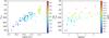Fig. 10

Central stellar mass density Σ_{1 kpc} versus stellar mass (left) and versus age (right). Left − The surface stellar mass density Σ_{1 kpc} within 1 kpc radius is plotted as a function of the stellar mass of the galaxies. The different colors mark the different mean age of the stellar population of the galaxies resulting from the best fitting to their SED. The large colored triangles represent the median age in four bins of stellar mass. Right− The central stellar mass density of cluster and field elliptical galaxies at z ~ 1.3 is plotted as a function of the age of their stellar population. Symbols are colored as a function of stellar mass.Errorbars are not shown to highlight the relationship between the quantities.

8. Summary and conclusions

In this paper we focused our investigation on the dependence of the population of elliptical galaxies at z ~ 1.3 and of their properties on the environment. We constructed two main samples of elliptical galaxies at the same redshift, the first one composed of 56 galaxies selected in three clusters at 1.2 <z< 1.4, the second one composed of 31 galaxies selected in the GOODS-South field at the same redshift. A third and larger (~180 galaxies) sample of field galaxies has been extracted from the COSMOS catalogs at slightly lower redshift (1.0 <z< 1.2) and used when it has been possible in some of the comparisons. Finally, a sample of ~220 ellipticals has been extracted from CANDELS at 1.2 <z< 1.4.

The selection of galaxies has been made on the basis of a pure morphological criterion based on the visual inspection of their luminosity profile in the ACS-F850LP image and of the residuals resulting from the profile fitting with a regular Sersic profile. The narrow redshift range adopted minimized the evolutionary effects, while the morphological selection of galaxies produced samples with the same composition, allowing us to single out the effect of the environment at a given morphology.

We compared the physical and structural properties of the population of elliptical galaxies in the two environments and we derived and compared the relationships among effective radius, surface brightness, stellar mass, and stellar mass density. Our main results can be summarized as follows:

The structure and the properties of cluster elliptical galaxies donot differ from those in the field. Cluster and field ellipticalgalaxies have the same median effective radius, the same massnormalized radius, and the same stellar mass density at fixedmass.
Cluster and field elliptical galaxies at z ~ 1.3 follow the same Kormendy (size-surface brightness) relation with a slope β ≃ 3.0. They also follow the same size-mass relation and the same size-mass density relations. The comparison of our data with those from the literature at the same redshift and with comparable selection criteria shows excellent agreement.
The population of cluster elliptical galaxies differs from the one in the field for high-mass and large elliptical galaxies. Indeed, there is a significant lack of massive (ℳ_∗> 2 × 10¹¹) M_⊙ and large (R_e> 4−5 kpc) elliptical galaxies in the field with respect to the cluster. Nonetheless, at ℳ_∗< 2 × 10¹¹M_⊙, the two populations are similar. There seems to be also a lack of elliptical galaxies in the field which are as old as the oldest ellipticals in cluster.

Hence, we do not find a dependence of the structure of elliptical galaxies on the environment where they belong, contrary to what has been predicted by some recent simulations. The above results show that the structure and the shaping of elliptical galaxies at z ~ 1.3 do not depend on the environment where they belong. However, they suggest that a dense environment is more efficient in assembling high-mass elliptical galaxies.

From the study of the scaling relations, we obtained the following results:

The size-mass relation is only coarselybest fitted by a single power law of the form $R_{e} \propto ℳ_{*}^{0.5}$ $\hbox{$R_{\rm e}\propto\mathcal{M}_*^{0.5}$}$ . We find a transition mass m_t ~ 2−3 × 10¹⁰M_⊙, in agreement with local studies, that defines two different regimes of the size-mass relation. Above this mass, the relation is steeper ( $R_{e} \propto ℳ_{*}^{0.64}$ $\hbox{$R_{\rm e}\propto\mathcal{M}_*^{0.64}$}$ ), while below this mass the relation gets flat ( $R_{e} \propto ℳ_{*}^{-0.13}$ $\hbox{$R_{\rm e}\propto\mathcal{M}_*^{-0.13}$}$ ), and the effective radius is nearly constant at ~1 kpc. The transition mass marks the mass at which a galaxy can reach the maximum stellar mass density within the effective radius.
The stellar mass density within the effective radius is tightly correlated with the effective radius. This size-effective mass density relation is best fitted by $Σ_{R_{e}} \propto R_{e}^{-1.2}$ $\hbox{$\Sigma_{R_{\rm e}}\propto R_{\rm e}^{-1.2}$}$ in agreement with the Kormendy relation. Galaxies with high or low effective stellar mass densities can be realized independently of the environment in which they reside and almost independently of their mass. The data show that a galaxy cannot occupy any locus in the [Σ_{R_e},ℳ_∗] plane but that a Zone of Exclusion, as the one defined by the early-type galaxies in the local Universe, exists at z ~ 1.3.
The central stellar mass density within 1 kpc radius is tightly correlated with mass and well fitted by $Σ_{1 kpc} \propto ℳ_{*}^{0.64}$ $\hbox{$\Sigma_{1\,{\rm kpc}}\propto\mathcal{M}_*^{0.64}$}$ , as previously found, at masses larger than m_t. At lower masses, the relation steepens with $Σ_{1 kpc} \propto ℳ_{*}^{1.07}$ $\hbox{$\Sigma_{1\,{\rm kpc}}\propto\mathcal{M}_*^{1.07}$}$ . We find that the central mass density is also correlated with the age of the stellar population such that the higher the central stellar mass density, the older the age, the higher the mass.

High mass galaxies are characterized by correspondingly high central stellar mass densities and old stellar population. The scaling of the central mass density with mass suggests that the process of assembly and of shaping of elliptical galaxies does not depend on the mass, at least in the mass range considered. These correlations taken all together, are indicative of the close connection of the central regions of the galaxies to the earliest phases of formation. The central regions of elliptical galaxies most probably store the information on their assembly, retain memory of the initial conditions, and are strictly connected to the bulk of their stellar mass growth. The outer regions (effective stellar mass density and effective radius) instead, store the information on the (subsequent) events that the galaxy may have experienced and that have affected the outer structure, but not its mass.

¹

https://rainbowx.fis.ucm.es/Rainbow_navigator_public/.

Acknowledgments

We are grateful to the anonymous referee for the constructive comments and suggestions. PS wishes to thank Stefano Andreon for the usefull comments. This work is based on data collected at the European Southern Observatory (ESO) telescopes (Prog. ID 084.A-0214(A), 60.A-9284(H)) and with the NASA/ESA Hubble Space Telescope, obtained from the data archive at ESO and at the Space Telescope Science Institute which is operated by the Association of Universities for Research in Astronomy. This work is also based on observations carried out at the Large Binocular Telescope (LBT; Prog. ID 19_2014). The LBT is an international collaboration among institutions in the United States, Italy, and Germany. We acknowledge the support from the LBT-Italian Coordination Facility for the execution of observations, data distribution, and reduction. This work made use of the Rainbow Cosmological Surveys Database, which is operated by the Universidad Complutense de Madrid (UCM), partnered with the University of California Observatories at Santa Cruz (UCO/Lick,UCSC).

References

Abazajian, K. N., Adelman-McCarthy, J. K., Agüeros, M. A., et al. 2009, ApJS, 182, 543 [NASA ADS] [CrossRef] [Google Scholar]
Allen, R. J., Kacprzak, G. G., Spitler, L. R., et al. 2015, ApJ, 806, 3 [NASA ADS] [CrossRef] [Google Scholar]
Andreon, S., Valtchanov, I., Jones, L. R., et al. 2005, MNRAS, 359, 1250 [NASA ADS] [CrossRef] [Google Scholar]
Bai, L., Yee, H. K. C., Yan, R., et al. 2014, ApJ, 789, 134 [NASA ADS] [CrossRef] [Google Scholar]
Bamford, S. P., Nichol, R. C., Baldry, I. K., et al. 2009, MNRAS, 393, 1324 [NASA ADS] [CrossRef] [Google Scholar]
Barro, G., Faber, S. M., Pérez-González, P. G., et al. 2013, ApJ, 765, 104 [NASA ADS] [CrossRef] [Google Scholar]
Bender, R., Burstein, D., & Faber, S. M. 1992, ApJ, 399, 462 [NASA ADS] [CrossRef] [Google Scholar]
Bernardi, M., Shankar, F., Hyde, J. B., et al. 2010, MNRAS, 404, 2087 [NASA ADS] [Google Scholar]
Bernardi, M., Roche, N., Shankar, F., & Sheth, R. K. 2011, MNRAS, 412, L6 [NASA ADS] [CrossRef] [Google Scholar]
Bernardi, M., Meert, A., Vikram, V., et al. 2014, MNRAS, 443, 874 [NASA ADS] [CrossRef] [Google Scholar]
Bertin, E., & Arnouts, S. 1996, A&AS, 117, 393 [NASA ADS] [CrossRef] [EDP Sciences] [Google Scholar]
Beutler, F., Blake, C., Colless, M., et al. 2013, MNRAS, 429, 3604 [NASA ADS] [CrossRef] [Google Scholar]
Bezanson, R., van Dokkum, P., van de Sande, J., Franx, M., & Kriek, M. 2013, ApJ, 764, L8 [NASA ADS] [CrossRef] [Google Scholar]
Bezanson, R., Franx, M., & van Dokkum, P. G. 2015, ApJ, 799, 148 [NASA ADS] [CrossRef] [Google Scholar]
Bildfell, C., Hoekstra, H., Babul, A., & Mahdavi, A. 2008, MNRAS, 389, 1637 [NASA ADS] [CrossRef] [Google Scholar]
Bolzonella, M., Miralles, J.-M., & Pelló, R. 2000, A&A, 363, 476 [NASA ADS] [Google Scholar]
Boselli, A., & Gavazzi, G. 2006, PASP, 118, 517 [NASA ADS] [CrossRef] [Google Scholar]
Boselli, A., & Gavazzi, G. 2014, A&ARv, 22, 74 [NASA ADS] [CrossRef] [Google Scholar]
Brammer, G. B., van Dokkum, P. G., Franx, M., et al. 2012, ApJS, 200, 13 [Google Scholar]
Bremer, M. N., Valtchanov, I., Willis, J., et al. 2006, MNRAS, 371, 1427 [NASA ADS] [CrossRef] [Google Scholar]
Bruzual, G., & Charlot, S. 2003, MNRAS, 344, 1000 [NASA ADS] [CrossRef] [Google Scholar]
Burstein, D., Bender, R., Faber, S., & Nolthenius, R. 1997, AJ, 114, 1365 [NASA ADS] [CrossRef] [Google Scholar]
Calvi, R., Poggianti, B. M., & Vulcani, B. 2011, MNRAS, 416, 727 [NASA ADS] [Google Scholar]
Calzetti, D., Armus, L., Bohlin, R. C., et al. 2000, ApJ, 533, 682 [NASA ADS] [CrossRef] [Google Scholar]
Capaccioli, M., & Corwin, Jr., H. G. 1989, Adv. Ser. Astrophys. Cosmol., 4 [Google Scholar]
Cappellari, M., McDermid, R. M., Alatalo, K., et al. 2013a, MNRAS, 432, 1862 [NASA ADS] [CrossRef] [Google Scholar]
Cappellari, M., Scott, N., Alatalo, K., et al. 2013b, MNRAS, 432, 1709 [NASA ADS] [CrossRef] [Google Scholar]
Cassata, P., Giavalisco, M., Guo, Y., et al. 2011, ApJ, 743, 96 [NASA ADS] [CrossRef] [Google Scholar]
Chabrier, G. 2003, PASP, 115, 763 [NASA ADS] [CrossRef] [Google Scholar]
Chan, J. C. C., Beifiori, A., Mendel, J. T., et al. 2016, MNRAS, 458, 3181 [NASA ADS] [CrossRef] [Google Scholar]
Cimatti, A., Nipoti, C., & Cassata, P. 2012, MNRAS, 422, L62 [NASA ADS] [CrossRef] [Google Scholar]
Ciotti, L. 1991, A&A, 249, 99 [NASA ADS] [Google Scholar]
Cooper, M. C., Griffith, R. L., Newman, J. A., et al. 2012, MNRAS, 419, 3018 [NASA ADS] [CrossRef] [Google Scholar]
Dahlen, T., Mobasher, B., Faber, S. M., et al. 2013, ApJ, 775, 93 [Google Scholar]
Damjanov, I., Geller, M. J., Zahid, H. J., & Hwang, H. S. 2015, ApJ, 806, 158 [NASA ADS] [CrossRef] [Google Scholar]
Davies, L. J. M., Driver, S. P., Robotham, A. S. G., et al. 2015, MNRAS, 447, 1014 [NASA ADS] [CrossRef] [Google Scholar]
De Lucia, G., Springel, V., White, S. D. M., Croton, D., & Kauffmann, G. 2006, MNRAS, 366, 499 [NASA ADS] [CrossRef] [Google Scholar]
De Propris, R., Bremer, M. N., & Phillipps, S. 2015, MNRAS, 450, 1268 [NASA ADS] [CrossRef] [Google Scholar]
Delaye, L., Huertas-Company, M., Mei, S., et al. 2014, MNRAS, 441, 203 [NASA ADS] [CrossRef] [Google Scholar]
di Serego Alighieri, S., Vernet, J., Cimatti, A., et al. 2005, A&A, 442, 125 [NASA ADS] [CrossRef] [EDP Sciences] [Google Scholar]
D’Onofrio, M., Fasano, G., Varela, J., et al. 2008, ApJ, 685, 875 [NASA ADS] [CrossRef] [Google Scholar]
Dressler, A. 1980, ApJ, 236, 351 [NASA ADS] [CrossRef] [Google Scholar]
Fang, J. J., Faber, S. M., Koo, D. C., & Dekel, A. 2013, ApJ, 776, 63 [NASA ADS] [CrossRef] [Google Scholar]
Fasano, G., Poggianti, B. M., Couch, W. J., et al. 2000, ApJ, 542, 673 [NASA ADS] [CrossRef] [Google Scholar]
Fasano, G., Marmo, C., Varela, J., et al. 2006, A&A, 445, 805 [NASA ADS] [CrossRef] [EDP Sciences] [Google Scholar]
Gargiulo, A., Haines, C. P., Merluzzi, P., et al. 2009, MNRAS, 397, 75 [NASA ADS] [CrossRef] [Google Scholar]
Gargiulo, A., Saracco, P., & Longhetti, M. 2011, MNRAS, 412, 1804 [NASA ADS] [CrossRef] [Google Scholar]
Gargiulo, A., Saracco, P., Longhetti, M., La Barbera, F., & Tamburri, S. 2012, MNRAS, 425, 2698 [NASA ADS] [CrossRef] [Google Scholar]
Gargiulo, A., Saracco, P., Tamburri, S., Lonoce, I., & Ciocca, F. 2016, A&A, 592, A132 [NASA ADS] [CrossRef] [EDP Sciences] [Google Scholar]
Gebhardt, K., Faber, S. M., Koo, D. C., et al. 2003, ApJ, 597, 239 [NASA ADS] [CrossRef] [Google Scholar]
Giavalisco, M., Ferguson, H. C., Koekemoer, A. M., et al. 2004, ApJ, 600, L93 [NASA ADS] [CrossRef] [Google Scholar]
Goto, T., Yamauchi, C., Fujita, Y., et al. 2003, MNRAS, 346, 601 [NASA ADS] [CrossRef] [Google Scholar]
Graham, A. W. 2013, Elliptical and Disk Galaxy Structure and Modern Scaling Laws, eds. T. D. Oswalt, & W. C. Keel, 91 [Google Scholar]
Graham, A. W., Merritt, D., Moore, B., Diemand, J., & Terzić, B. 2006, AJ, 132, 2711 [NASA ADS] [CrossRef] [Google Scholar]
Grazian, A., Fontana, A., de Santis, C., et al. 2006, A&A, 449, 951 [NASA ADS] [CrossRef] [EDP Sciences] [Google Scholar]
Greggio, L., & Renzini, A. 2011, Stellar Populations, A User Guide from Low to High Redshift [Google Scholar]
Grogin, N. A., Kocevski, D. D., Faber, S. M., et al. 2011, ApJS, 197, 35 [NASA ADS] [CrossRef] [Google Scholar]
Guglielmo, V., Poggianti, B. M., Moretti, A., et al. 2015, MNRAS, 450, 2749 [NASA ADS] [CrossRef] [Google Scholar]
Guo, Y., McIntosh, D. H., Mo, H. J., et al. 2009, MNRAS, 398, 1129 [NASA ADS] [CrossRef] [Google Scholar]
Guo, Y., Giavalisco, M., Cassata, P., et al. 2011, ApJ, 735, 18 [NASA ADS] [CrossRef] [Google Scholar]
Guo, Y., Ferguson, H. C., Giavalisco, M., et al. 2013, ApJS, 207, 24 [NASA ADS] [CrossRef] [Google Scholar]
Haines, C. P., Pereira, M. J., Smith, G. P., et al. 2013, ApJ, 775, 126 [NASA ADS] [CrossRef] [EDP Sciences] [Google Scholar]
Hamabe, M., & Kormendy, J. 1987, in Structure and Dynamics of Elliptical Galaxies, ed. P. T. de Zeeuw, IAU Symp., 127, 379 [Google Scholar]
Holden, B. P., Blakeslee, J. P., Postman, M., et al. 2005, ApJ, 626, 809 [NASA ADS] [CrossRef] [Google Scholar]
Holden, B. P., Illingworth, G. D., Franx, M., et al. 2007, ApJ, 670, 190 [NASA ADS] [CrossRef] [Google Scholar]
Huertas-Company, M., Mei, S., Shankar, F., et al. 2013a, MNRAS, 428, 1715 [NASA ADS] [CrossRef] [Google Scholar]
Huertas-Company, M., Shankar, F., Mei, S., et al. 2013b, ApJ, 779, 29 [NASA ADS] [CrossRef] [Google Scholar]
Huertas-Company, M., Pérez-González, P. G., Mei, S., et al. 2015, ApJ, 809, 95 [NASA ADS] [CrossRef] [Google Scholar]
Hyde, J. B., & Bernardi, M. 2009, MNRAS, 396, 1171 [NASA ADS] [CrossRef] [Google Scholar]
Jørgensen, I., & Chiboucas, K. 2013, AJ, 145, 77 [NASA ADS] [CrossRef] [Google Scholar]
Jørgensen, I., Franx, M., & Kjaergaard, P. 1995, MNRAS, 273, 1097 [NASA ADS] [CrossRef] [Google Scholar]
Jørgensen, I., Chiboucas, K., Toft, S., et al. 2014, AJ, 148, 117 [NASA ADS] [CrossRef] [Google Scholar]
Kartaltepe, J. S., Mozena, M., Kocevski, D., et al. 2015, ApJS, 221, 11 [NASA ADS] [CrossRef] [Google Scholar]
Kauffmann, G., Heckman, T. M., White, S. D. M., et al. 2003, MNRAS, 341, 54 [Google Scholar]
Kelkar, K., Aragón-Salamanca, A., Gray, M. E., et al. 2015, MNRAS, 450, 1246 [NASA ADS] [CrossRef] [Google Scholar]
Khochfar, S., Emsellem, E., Serra, P., et al. 2011, MNRAS, 417, 845 [NASA ADS] [CrossRef] [Google Scholar]
Koekemoer, A. M., Aussel, H., Calzetti, D., et al. 2007, ApJS, 172, 196 [NASA ADS] [CrossRef] [Google Scholar]
Koekemoer, A. M., Faber, S. M., Ferguson, H. C., et al. 2011, ApJS, 197, 36 [NASA ADS] [CrossRef] [Google Scholar]
Kuntschner, H., Smith, R. J., Colless, M., et al. 2002, MNRAS, 337, 172 [NASA ADS] [CrossRef] [Google Scholar]
La Barbera, F., Busarello, G., Merluzzi, P., Massarotti, M., & Capaccioli, M. 2003, ApJ, 595, 127 [NASA ADS] [CrossRef] [Google Scholar]
La Barbera, F., de Carvalho, R. R., de La Rosa, I. G., et al. 2010, MNRAS, 408, 1313 [NASA ADS] [CrossRef] [Google Scholar]
Lani, C., Almaini, O., Hartley, W. G., et al. 2013, MNRAS, 435, 207 [NASA ADS] [CrossRef] [Google Scholar]
Lidman, C., Rosati, P., Tanaka, M., et al. 2008, A&A, 489, 981 [NASA ADS] [CrossRef] [EDP Sciences] [Google Scholar]
Lidman, C., Iacobuta, G., Bauer, A. E., et al. 2013, MNRAS, 433, 825 [NASA ADS] [CrossRef] [Google Scholar]
Lin, Y.-T., Mohr, J. J., & Stanford, S. A. 2004, ApJ, 610, 745 [NASA ADS] [CrossRef] [Google Scholar]
Longhetti, M., & Saracco, P. 2009, MNRAS, 394, 774 [NASA ADS] [CrossRef] [Google Scholar]
Lonoce, I., Longhetti, M., Saracco, P., Gargiulo, A., & Tamburri, S. 2014, MNRAS, 444, 2048 [NASA ADS] [CrossRef] [Google Scholar]
Maltby, D. T., Aragón-Salamanca, A., Gray, M. E., et al. 2010, MNRAS, 402, 282 [NASA ADS] [CrossRef] [Google Scholar]
Mei, S., Holden, B. P., Blakeslee, J. P., et al. 2009, ApJ, 690, 42 [NASA ADS] [CrossRef] [Google Scholar]
Mei, S., Stanford, S. A., Holden, B. P., et al. 2012, ApJ, 754, 141 [Google Scholar]
Menci, N., Rosati, P., Gobat, R., et al. 2008, ApJ, 685, 863 [NASA ADS] [CrossRef] [Google Scholar]
Moran, S. M., Ellis, R. S., Treu, T., et al. 2007, ApJ, 671, 1503 [NASA ADS] [CrossRef] [Google Scholar]
Moresco, M., Pozzetti, L., Cimatti, A., et al. 2013, A&A, 558, A61 [NASA ADS] [CrossRef] [EDP Sciences] [Google Scholar]
Muzzin, A., Wilson, G., Yee, H. K. C., et al. 2012, ApJ, 746, 188 [NASA ADS] [CrossRef] [Google Scholar]
Muzzin, A., Marchesini, D., Stefanon, M., et al. 2013, ApJS, 206, 8 [Google Scholar]
Naab, T., Johansson, P. H., & Ostriker, J. P. 2009, ApJ, 699, L178 [NASA ADS] [CrossRef] [Google Scholar]
Newman, A. B., Ellis, R. S., Bundy, K., & Treu, T. 2012, ApJ, 746, 162 [NASA ADS] [CrossRef] [Google Scholar]
Newman, A. B., Ellis, R. S., Andreon, S., et al. 2014, ApJ, 788, 51 [NASA ADS] [CrossRef] [Google Scholar]
Nonino, M., Dickinson, M., Rosati, P., et al. 2009, ApJS, 183, 244 [NASA ADS] [CrossRef] [Google Scholar]
Oemler, Jr., A. 1974, ApJ, 194, 1 [NASA ADS] [CrossRef] [Google Scholar]
Pannella, M., Gabasch, A., Goranova, Y., et al. 2009, ApJ, 701, 787 [NASA ADS] [CrossRef] [Google Scholar]
Papovich, C., Bassett, R., Lotz, J. M., et al. 2012, ApJ, 750, 93 [NASA ADS] [CrossRef] [Google Scholar]
Peng, C. Y., Ho, L. C., Impey, C. D., & Rix, H. 2002, AJ, 124, 266 [NASA ADS] [CrossRef] [Google Scholar]
Poggianti, B. M., Calvi, R., Bindoni, D., et al. 2013a, ApJ, 762, 77 [NASA ADS] [CrossRef] [Google Scholar]
Poggianti, B. M., Moretti, A., Calvi, R., et al. 2013b, ApJ, 777, 125 [NASA ADS] [CrossRef] [Google Scholar]
Postman, M., & Geller, M. J. 1984, ApJ, 281, 95 [NASA ADS] [CrossRef] [Google Scholar]
Postman, M., Franx, M., Cross, N. J. G., et al. 2005, ApJ, 623, 721 [NASA ADS] [CrossRef] [Google Scholar]
Pozzetti, L., Bolzonella, M., Zucca, E., et al. 2010, A&A, 523, A13 [NASA ADS] [CrossRef] [EDP Sciences] [Google Scholar]
Raichoor, A., Mei, S., Nakata, F., et al. 2011, ApJ, 732, 12 [NASA ADS] [CrossRef] [Google Scholar]
Raichoor, A., Mei, S., Stanford, S. A., et al. 2012, ApJ, 745, 130 [NASA ADS] [CrossRef] [Google Scholar]
Reda, F. M., Forbes, D. A., Beasley, M. A., O’Sullivan, E. J., & Goudfrooij, P. 2004, MNRAS, 354, 851 [NASA ADS] [CrossRef] [Google Scholar]
Renzini, A. 2006, ARA&A, 44, 141 [NASA ADS] [CrossRef] [Google Scholar]
Rettura, A., Rosati, P., Nonino, M., et al. 2010, ApJ, 709, 512 [NASA ADS] [CrossRef] [Google Scholar]
Rettura, A., Mei, S., Stanford, S. A., et al. 2011, ApJ, 732, 94 [NASA ADS] [CrossRef] [Google Scholar]
Rosati, P., Tozzi, P., Gobat, R., et al. 2009, A&A, 508, 583 [NASA ADS] [CrossRef] [EDP Sciences] [Google Scholar]
Saglia, R. P., Sánchez-Blázquez, P., Bender, R., et al. 2010, A&A, 524, A6 [NASA ADS] [CrossRef] [EDP Sciences] [Google Scholar]
Santini, P., Fontana, A., Grazian, A., et al. 2009, A&A, 504, 751 [NASA ADS] [CrossRef] [EDP Sciences] [Google Scholar]
Santini, P., Ferguson, H. C., Fontana, A., et al. 2015, ApJ, 801, 97 [NASA ADS] [CrossRef] [Google Scholar]
Saracco, P., Longhetti, M., & Andreon, S. 2009, MNRAS, 392, 718 [NASA ADS] [CrossRef] [Google Scholar]
Saracco, P., Gargiulo, A., & Longhetti, M. 2012, MNRAS, 422, 3107 [NASA ADS] [CrossRef] [Google Scholar]
Saracco, P., Casati, A., Gargiulo, A., et al. 2014, A&A, 567, A94 [NASA ADS] [CrossRef] [EDP Sciences] [Google Scholar]
Sargent, M. T., Carollo, C. M., Lilly, S. J., et al. 2007, ApJS, 172, 434 [NASA ADS] [CrossRef] [Google Scholar]
Scarlata, C., Carollo, C. M., Lilly, S., et al. 2007, ApJS, 172, 406 [NASA ADS] [CrossRef] [Google Scholar]
Schade, D., Carlberg, R. G., Yee, H. K. C., Lopez-Cruz, O., & Ellingson, E. 1996, ApJ, 464, L63 [NASA ADS] [CrossRef] [Google Scholar]
Shankar, F., Lapi, A., Salucci, P., De Zotti, G., & Danese, L. 2006, ApJ, 643, 14 [NASA ADS] [CrossRef] [MathSciNet] [Google Scholar]
Shankar, F., Marulli, F., Bernardi, M., et al. 2013, MNRAS, 428, 109 [NASA ADS] [CrossRef] [Google Scholar]
Shankar, F., Guo, H., Bouillot, V., et al. 2014a, ApJ, 797, L27 [NASA ADS] [CrossRef] [Google Scholar]
Shankar, F., Mei, S., Huertas-Company, M., et al. 2014b, MNRAS, 439, 3189 [NASA ADS] [CrossRef] [Google Scholar]
Skelton, R. E., Whitaker, K. E., Momcheva, I. G., et al. 2014, ApJS, 214, 24 [Google Scholar]
Smith, G. P., Treu, T., Ellis, R. S., Moran, S. M., & Dressler, A. 2005, ApJ, 620, 78 [NASA ADS] [CrossRef] [Google Scholar]
Stanford, S. A., Elston, R., Eisenhardt, P. R., et al. 1997, AJ, 114, 2232 [NASA ADS] [CrossRef] [Google Scholar]
Strazzullo, V., Rosati, P., Pannella, M., et al. 2010, A&A, 524, A17 [NASA ADS] [CrossRef] [EDP Sciences] [Google Scholar]
Strazzullo, V., Gobat, R., Daddi, E., et al. 2013, ApJ, 772, 118 [NASA ADS] [CrossRef] [Google Scholar]
Tacchella, S., Carollo, C. M., Renzini, A., et al. 2015, Science, 348, 314 [NASA ADS] [CrossRef] [Google Scholar]
Tacchella, S., Dekel, A., Carollo, C. M., et al. 2016, MNRAS, 458, 242 [NASA ADS] [CrossRef] [Google Scholar]
Tamburri, S., Saracco, P., Longhetti, M., et al. 2014, A&A, 570, A102 [NASA ADS] [CrossRef] [EDP Sciences] [Google Scholar]
Tanaka, M., De Breuck, C., Venemans, B., & Kurk, J. 2010, A&A, 518, A18 [NASA ADS] [CrossRef] [EDP Sciences] [Google Scholar]
Tanaka, M., Finoguenov, A., Lilly, S. J., et al. 2012, PASJ, 64 [Google Scholar]
Tanaka, M., Toft, S., Marchesini, D., et al. 2013, ApJ, 772, 113 [NASA ADS] [CrossRef] [Google Scholar]
Tasca, L. A. M., Kneib, J.-P., Iovino, A., et al. 2009, A&A, 503, 379 [NASA ADS] [CrossRef] [EDP Sciences] [Google Scholar]
Taylor, E. N., Franx, M., Brinchmann, J., van der Wel, A., & van Dokkum, P. G. 2010, ApJ, 722, 1 [NASA ADS] [CrossRef] [Google Scholar]
Thomas, D., Maraston, C., Bender, R., & Mendes de Oliveira, C. 2005, ApJ, 621, 673 [NASA ADS] [CrossRef] [Google Scholar]
Thomas, D., Maraston, C., Schawinski, K., Sarzi, M., & Silk, J. 2010, MNRAS, 404, 1775 [NASA ADS] [Google Scholar]
Tran, K.-V. H., Simard, L., Zabludoff, A. I., & Mulchaey, J. S. 2001, ApJ, 549, 172 [NASA ADS] [CrossRef] [Google Scholar]
Treu, T., Ellis, R. S., Kneib, J.-P., et al. 2003, ApJ, 591, 53 [NASA ADS] [CrossRef] [Google Scholar]
Valentinuzzi, T., Fritz, J., Poggianti, B. M., et al. 2010, ApJ, 712, 226 [NASA ADS] [CrossRef] [Google Scholar]
van der Burg, R. F. J., Hoekstra, H., Muzzin, A., et al. 2015, A&A, 577, A19 [NASA ADS] [CrossRef] [EDP Sciences] [Google Scholar]
van der Wel, A., Holden, B. P., Franx, M., et al. 2007, ApJ, 670, 206 [NASA ADS] [CrossRef] [Google Scholar]
van der Wel, A., Bell, E. F., Häussler, B., et al. 2012, ApJS, 203, 24 [NASA ADS] [CrossRef] [Google Scholar]
van Dokkum, P. G., Stanford, S. A., Holden, B. P., et al. 2001, ApJ, 552, L101 [NASA ADS] [CrossRef] [Google Scholar]
van Dokkum, P. G., Whitaker, K. E., Brammer, G., et al. 2010, ApJ, 709, 1018 [NASA ADS] [CrossRef] [Google Scholar]
von der Linden, A., Best, P. N., Kauffmann, G., & White, S. D. M. 2007, MNRAS, 379, 867 [NASA ADS] [CrossRef] [Google Scholar]
Vulcani, B., Poggianti, B. M., Fritz, J., et al. 2015, ApJ, 798, 52 [NASA ADS] [CrossRef] [Google Scholar]
Vulcani, B., Marchesini, D., De Lucia, G., et al. 2016, ApJ, 816, 86 [NASA ADS] [CrossRef] [Google Scholar]
Weinmann, S. M., Kauffmann, G., van den Bosch, F. C., et al. 2009, MNRAS, 394, 1213 [NASA ADS] [CrossRef] [Google Scholar]
Zahid, H. J., Damjanov, I., Geller, M. J., Hwang, H. S., & Fabricant, D. G. 2016, ApJ, 821, 101 [NASA ADS] [CrossRef] [Google Scholar]
Ziegler, B. L., Saglia, R. P., Bender, R., et al. 1999, A&A, 346, 13 [NASA ADS] [Google Scholar]

Appendix A: Data description

Appendix A.1: Cluster data

We describe here the data available and used for the three clusters.

XMM J2235-2557 – The HST data are composed of optical ACS observations in the filters F775W (5060 s) and F850LP (6240 s), and of near-IR WFC3 observations in the filter F160W (1200 s) described in Rosati et al. (2009) and in Strazzullo et al. (2010). The ACS and the WFC3 images used here have a pixel scale of 0.05 arcsec/pixel and a resolution of FWHM_F850 ≃ 0.11 arcsec and of FWHM_F160 ≃ 0.2 arcsec. VLT data include VIMOS U-band observations (21000 s, FWHM ≃ 0.8 arcsec, Nonino et al. 2009), and HAWKI J- and K-band observations (~10 500 s, Lidman et al. 2008, 2013) characterized by a FWHM_J ≃ 0.5 arcsec and FWHM_K ≃ 0.35 arcsec. Spitzer data are composed of fully co-added IRAC mosaics (0.6 arcsec/pixel) in the four bandpasses 3.6 μm, 4.5 μm, 5.8 μm (≃2100 s), and 8.0 μm (≃1900 s). Spectroscopic redshifts for five galaxies have been derived from Rosati et al. (2009). A detailed description of this data set and of this sample is provided by Ciocca et al. (2016, in prep).

RDCSJ0848+4453 – The HST data includes ACS observations (0.05 arcsec/pixel) in the filters F775W (7300 s) and F850LP (12 200 s, FWHM ≃ 0.12 arcsec) described in Postman et al. (2005), and of near-IR NICMOS-NIC3 observations (0.2 arcsec/pixel) in the filter F160W (11 200 s; FWHM ≃ 0.22 arcsec) described in van Dokkum et al. (2001). LBT data are composed of LBC observations in the U,B,V, and R filters (~14 000 s each; see Saracco et al. 2014) and are characterized by a FWHM ~ 1.0 arcsec. Spitzer fully co-added mosaics (0.6 arcsec/pixel) in the four IRAC bandapasses 3.6 μm and 5.8 μm (~2200 s), 4.5 μm, and 8.0 μm (≃1900 s) complete this data set. Spectroscopic redshifts are available for 12 galaxies from Jørgensen et al. (2014) and van Dokkum et al. (2001). A complete and detailed description of this data set is provided by Saracco et al. (2014).

XLSSJ0223-0436 − The data set used for this cluster is composed of HST-ACS images in the F775W (2000 s) and F850LP (6000 s) filters, proprietary LBT-LBC observations (Prog. ID 19_2014) in the V and I filters (~6300 s and ~4400 s respectively, FWHM ≃ 0.7 arcsec), VLT-HAWKI observations in the J and K filters (~3000 s each, FWHM ≃ 0.35 arcsec), and Spitzer fully co-added mosaics (0.6 arcsec/pixel) in the four IRAC bandapasses 3.6 μm, 4.5 μm, 5.8 μm, and 8.0 μm. Spectroscopic redshift are available for about 14 galaxies from Bremer et al. (2006) and Saracco et al. (in prep.), where a detailed description of this data set is also given.

In Fig. A.1 we show the comparison between the photometric redshift and the spectrosopic redshift for the elliptical galaxies spectroscopically confirmed cluster members. The photometric redshift accuracy is σ_{Δz/ (1 + z_s)} = 0.04 (0.02 using the normalized median absolute deviation).

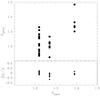Fig. A.1

Comparison between photometric and spectroscopic redshifts for the elliptical cluster members.

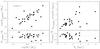Fig. A.2

Left − stellar mass from CANDELS catalog compared with the stellar mass we estimated for the 31 galaxies of the GOODS-S field in common. Right − effective radius in the F160W band from CANDELS catalog plotted as a function of the effective radius we estimated in the F850LP band for the 31 galaxies in the GOODS-S field.

Appendix A.2: CANDELS data sample

In order to homogenize as much as possible the parameters of CANDELS galaxies with those of our samples, we considered the 31 elliptical galaxies selected in the GOODS-S field in common with the CANDELS catalog. We first checked the agreement between the morphological classification and between the main parameters used in this analysis: the stellar mass and the effective radius.

As far as the morphological classification is concerned, all the 31 galaxies we classified as ellipticals in the F850LP images have dominant class =0, that is, they are classified spheroids also in the CANDELS catalog. Four of them have the flag parameter value on the goodness of the Galfit fit parameter_gfit_f_h=1 suggesting that the fitting to their profile in the F160W band is not very good.

In Fig. A.2 (left panel) we compare the stellar masses of CANDELS catalog with our estimate for the 31 galaxies in common. The agreement is rather good; we estimate a small offset of about a factor 0.05dex in the sense that the stellar masses in the CANDELS catalog seems to be slightly larger than our estimates. We applied this small scaling to the CANDELS data.

In the right panel of Fig. A.2 we compare the effective radii in the F160W band from CANDELS catalog with those we estimated in the F850LP band. The agreement is rather good at small radii while the scatter is large at larger radii. We do not clearly detect the 10−20% offset between the effective radii estimated in the two bands found in other works (e.g., Gargiulo et al. 2012; Cassata et al. 2011). Possibly, a trend with the radius (the larger the F850LP band radius, the lower the ratio R_e(F160)/R_e(850)) is present, however, the small statistic and the large scatter do not allow us to confirm this. For these reasons, we did not apply any scaling to the effective radii of CANDELS sample.

Appendix B: Cluster and field data samples

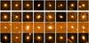Fig. B.1

F850LP band images for a representative sample of elliptical galaxies in the field and cluster samples. Each row shows the 3×3 arcsec width images for some elliptical galaxies in the GOODS-S field (top row), in the XMM J2235 cluster (second row), in the RDCSJ0848 cluster (third row), and in the XLSSJ0223 cluster (bottom row).

In this appendix we report the structural and the physical parameters we derived for the cluster sample (Table B.1) and for the field sample (Table B.2). Namely: Sersic index n, axial ratio b/a, apparent magnitude F850_fit, and effective radius R_e [kpc] as derived from the fitting to the surface brightness profile in the F850LP image; effective surface brightness $⟨ μ ⟩_{e}^{B}$ $\hbox{$\langle \mu\rangle_{\rm e}^B$}$ , age of the stellar population, and stellar mass ℳ_∗ fitting (see Sect. 3); stellar mass within 1 kpc radius ℳ_{1 kpc} and absolute magnitude M_B in the B-band. The error quoted for F850_fit is the square root of the quadratic sum of the photometric error with the Galfit error. The typical uncertainties (at one σ) affecting stellar masses and ages derived from the SED fitting are 15% and 20% respectively (25% for ages older than 3.5 Gyr). These uncertainties take into account only photometric errors. The term Ev_B is the luminosity evolution in the B band of the galaxy from its redshift to z = 0, according to its own age based on BC03 models. In Fig. B.1 we show the F850LP images for a representative sample of elliptical galaxies in the field and cluster samples.

Table B.1

Morphological parameters of cluster elliptical galaxies.

Table B.2

Morphological parameters of elliptical galaxies in the field.

Appendix C: Scaling relations: least square and orthogonal fitting

For the sake of completeness, in this appendix we summarize the best fitting relations we obtained with the classical least squares method, which minimizes the sum of the square of the residuals in the dependent variable Y from the line, and those obtained using the Person’s orthogonal regression line, which treats the variables symmetrically, minimizing the squares of the perpendicular distances from the point to the line. The best fitting parameters are listed in Table C.1 where, for each relation indicated in the first column, we report the values obtained with the least square fitting (second and third columns) and those obtained with the orthogonal fitting (fourth and fifth columns). In the last column we report the section in which the relations are derived and discussed and, where appropriate, the range of fitting.

The two methods provide slopes that differ at ~2σ for the Kormendy relation and the Σ_{R_e}−R_e relation, while for the size-mass and the Σ_{1 kpc}-ℳ_∗ the slopes are consistent within 1σ. It is worth noting that, in the presence of boundary conditions along the Y axis, as in the case of the fitting at masses larger or lower than m_t, the orthogonal fit is biased toward steeper slopes. This can be easily seen in Fig. 7 where the data close to the boundary affect asymmetrically the orthogonal regression lines in the two mass ranges. Boundary conditions should be applied orthogonally to the fit or treated through iterative routines, procedures that go beyond the scope of this work. Our aim is to show the presence of two different regimes in the size-mass relation and in the Σ_{1 kpc}−ℳ_∗ relation at masses lower and higher than a mass ℳ_∗ ≃ 2−3 × 10¹⁰M_⊙. It is important to note that, for the reasons above, the true slope of the relations will lie in between the one provided by the least square method, that can be considered as a lower limit, and the one provided by the orthogonal fit, that can be considered as an upper limit.

Table C.1

Scaling relations of elliptical galaxies at z ~ 1.3.

All Tables

Table 1

Kormendy relation of cluster and field ellipticals at z ~ 1.3.

In the text

Table B.1

Morphological parameters of cluster elliptical galaxies.

In the text

Table B.2

Morphological parameters of elliptical galaxies in the field.

In the text

Table C.1

Scaling relations of elliptical galaxies at z ~ 1.3.

In the text

All Figures

Fig. 1

Distribution of stellar mass and effective radius for cluster and field elliptical galaxies. Upper panel − distribution of the stellar mass ℳ_∗ (left) and of the effective radius R_e (right) for the 56 cluster elliptical galaxies (red shaded histograms) and the 31 elliptical galaxies in the GOODS-South field (blue shaded histograms). The lower panels show the comparison with the field elliptical galaxies selected in the COSMOS area (green histograms). The colored solid line marks the median values of the distributions (see text). The dotted line marks the reference values log ℳ_∗ = 11.1 M_⊙ and R_e = 4 kpc above which the distributions are significantly different. Lower panel − same as in the upper panel but in this case the distributions of the cluster ellipticals are compared with those of the elliptical galaxies selected from CANDELS (cyan histograms; see Sect. 2).

In the text

Fig. 2

Age distribution of cluster and field ellipticals. Left − the distribution of the age of the stellar population of field elliptical galaxies (blue shaded histogram) is compared with the age distribution of all the cluster ellipticals (red shaded histogram).The colored solid lines mark the median values of the distributions (see text). Right − same as left panel but in this case the comparison is made by considering field and cluster ellipticals in the same mass range, that is, by excluding cluster galaxies with masses larger than log (ℳ_∗) = 11.1 M_⊙.

In the text

Fig. 3

Distribution of mass-normalized radius and stellar mass density for cluster and field elliptical galaxies. Upper panel − distributions of the mass normalized radius (left) and of the effective stellar mass density Σ_{R_e} (right) for cluster (red histograms) and field elliptical galaxies in the GOODS-South field (blue histograms) and in the COSMOS area (green histograms). The effective radius R_e is normalized to the stellar mass $m_{*}^{0.5}$ $\hbox{$m_*^{0.5}$}$ where m_∗ = ℳ_∗/ 10¹¹M_⊙.Colored solid lines mark the median values of the distributions. The black dotted line marks the median value Σ_{R_e} = 2500 M_⊙ pc^-2 of the elliptical galaxies in cluster and in the GOODS-S field.Lower panel − same as in the upper panel but the comparison is made with the field elliptical galaxies selected in the CANDELS area (cyan histograms).

In the text

Fig. 4

Stellar mass distribution of compact and normal galaxies in field and cluster environment. Upper panel − the distribution of the stellar mass of normal elliptical galaxies (magenta histogram) in cluster is compared to the one of compact galaxies (cyan histogram) defined according to the criterion log $(ℳ_{*} / R_{e}^{1.5}) > 10.3$ $\hbox{$(\mathcal{M}_*/R_{\rm e}^{1.5})>10.3$}$ . Lower panel − same as for the upper panel but for field elliptical galaxies.

In the text

Fig. 5

Kormendy relation in the rest-frame B-band for cluster and field elliptical galaxies at z ≃ 1.3. Upper panel− the B-band surface brightness of the 17 galaxies in the cluster XMMU2235 at z ~ 1.39 (dark red filled squares), of the 16 galaxies in the RDCS0848 at z ~ 1.27 (brick red filled circles), and of the 23 galaxies in the cluster XLSS0223 at z ~ 1.22 (red filled triangles) are plotted as a function of their effective radius R_e at the redshift of the clusters. The three colored lines are the best fitting Kormendy relations to the three clusters reported in Table 1. The open symbols are the sample of early-type galaxies in the Linx clusters and groups studied by Raichoor et al. (2012). Lower panel: the surface brightness of the 56 cluster galaxies (red filled circles), of the 31 field galaxies at 1.2 <z< 1.45 in the GOODS-South region (blue filled squares), and of the 178 galaxies at 1.0 <z< 1.2 in the COSMOS area (green filled triangles) are plotted as a function of their effective radius. The red solid line and the blue dashed line are the best fitting relations obtained for cluster and GOODS-S field galaxies respectively, and are reported in Table 1. At the bottom of the figure, the mean age ⟨ age ⟩ [Gyr] of galaxies in the different intervals of effective radius together with its dispersion (σ) is reported.

In the text

Fig. 6

Effective radius-stellar mass relation for elliptical galaxies. Upper panel − the mass normalized radius $R_{e} / m_{*}^{0.5}$ $\hbox{$R_{\rm e}/m_*^{0.5}$}$ is plotted as a function of the stellar mass ℳ_∗. The filled symbols are the cluster ellipticals of our sample (red circles), the field ellipticals we selected at 1.2 <z< 1.45 in the GOODS-S field (blue squares), and the ellipticals at 1.0 <z< 1.2 in the COSMOS field (green crosses). Open symbols are data taken from Raichoor et al. (2012; R12, stars), from Delaye et al. (2014; D14, triangles), and from Valentinuzzi et al. (2010 V10, circles; see also Poggianti et al. 2013a). The green short-dashed line is $y = 1.3 [kpc] / m_{*}^{0.5} + c$ $\hbox{$y=1.3[{\rm kpc}]/m_*^{0.5}+c$}$ , the line below which there are no measured effective radii in the COSMOS catalog (Sargent et al. 2007). We report errorbars only in the lower panel just for clarity in the plot. Lower panel − the effective radius R_e is plotted versus the stellar mass. Symbols are as in the upper panel. The big black filled triangles are the median values of our sample of cluster and field ellipticals at z ~ 1.3. The long-dashed line is the best fitting relation $R_{e} \propto ℳ_{*}^{0.5}$ $\hbox{$R_{\rm e}\propto\mathcal{M}_*^{0.5}$}$ over the whole mass range.

In the text

Fig. 7

Effective radius-stellar mass relation for elliptical galaxies. Filled symbols are field (squares) and cluster (circles) ellipticals of our sample. Empty symbols are as Fig. 6. The thick solid lines are the best fitting relations obtained with the least square fit for values lower and higher than ℳ_∗ = 2.5 × 10¹⁰M_⊙, $R_{e} = 26 \times ℳ_{*}^{- 0.13 \pm 0.2}$ $\hbox{$R_{\rm e}=26\times\mathcal{M}_*^{-0.13\,\pm\,0.2}$}$ , and $R_{e} = 2.77 \times 10^{-7} ℳ_{*}^{0.64 \pm 0.09}$ $\hbox{$R_{\rm e}=2.77\times10^{-7}\mathcal{M}_*^{0.64\pm0.09}$}$ respectively. The blue dashed line is the best fitting relations obtained in the two mass ranges using the orthogonal fit (see Appendix A), $R_{e} \propto ℳ_{*}^{- 0.3 \pm 0.2}$ $\hbox{$R_{\rm e}\propto\mathcal{M}_*^{-0.3\,\pm\,0.2}$}$ and $R_{e} \propto ℳ_{*}^{1.0 \pm 0.1}$ $\hbox{$R_{\rm e}\propto\mathcal{M}_*^{1.0\pm0.1}$}$ respectively. The gray dot-dashed line is the relation R_e = 0.53(ℳ_∗/ 3 × 10¹⁰)^-0.2(0.5 + 0.5(ℳ_∗/ 3 × 10¹⁰)^0.8)^0.119 defining the Zone of Exclusion (ZOE) as obtained by Cappellari et al. (2013a) and scaled by a factor $⟨ R_{e} / R_{e}^{maj} ⟩ = 0.76$ $\hbox{$ \langle R_{\rm e}/R_{\rm e}^{\rm maj} \rangle\,=\,0.76$}$ (see text). Open symbols represent the samples of Raichoor et al. (2012; stars, R12) and of Delaye et al. (2014; triangles, D14).Cyan crosses are elliptical galaxies selected from CANDELS.

In the text

Fig. 8

Stellar mass surface density versus effective radius and stellar mass. Upper panel − the effective stellar mass density within the effective radius $Σ_{R_{e}} = ℳ_{*} / 2 π R_{e}^{2}$ $\hbox{$\Sigma_{R_{\rm e}}=\mathcal{M}_*/2\pi R_{\rm e}^2$}$ , is plotted as a function of the effective radius R_e (left) and of the stellar mass ℳ_∗ (right). Blue filled squares are field ellipticals in the GOODS-S regions, green crosses are those in the COSMOS area, and red filled circles are cluster ellipticals. The black solid line is the best-fitting relation $Σ_{R_{e}} \propto R_{e}^{- 1.2 \pm 0.1}$ $\hbox{$\Sigma_{R_{\rm e}}\propto R_{\rm e}^{-1.2\pm0.1}$}$ (see Appendix A for the orthogonal fit). The green dashed line in the right panel shows the stellar mass density as a function of mass for a constant value of R_e = 1.3 kpc (marked on the left panel), corresponding to the limiting value ~0.17 arcsec adopted for the effective radius in the COSMOS catalog of Scarlata et al. (2007). The gray dot-dashed line marks the Zone of Exclusion (ZOE) as defined in Sect. 6.1. The open stars are the early-type galaxies selected by Raichoor et al. (2011; R11) in groups and clusters at z ~ 1.27. The open triangles are the cluster elliptical galaxies at 1.22 <z< 1.4 studied by Delaye et al. (2014; D14).The cyan crosses are the elliptical galaxies from CANDELS. Lower panel − the central stellar mass density calculated within 1 kpc radius (Σ_{1 kpc}) is plotted as a function of the effective radius (left) and of the stellar mass (right). Symbols are as in the upper panel. The solid black line is the best-fitting broken power law $Σ_{1 kpc} \propto ℳ_{*}^{(0.64 \pm 0.06)}$ $\hbox{$\Sigma_{1\,{\rm kpc}}\propto\mathcal{M}_*^{(0.64\pm0.06)}$}$ for ℳ_∗>m_t and $Σ_{1 kpc} \propto ℳ_{*}^{(1.07 \pm 0.1)}$ $\hbox{$\Sigma_{1\,{\rm kpc}}\propto\mathcal{M}_*^{(1.07\pm0.1)}$}$ for ℳ_∗<m_t, with m_t = 2.5 × 10¹⁰M_⊙. The gray dashed line is the relation found by Tacchella et al. (2016) with their model of mass growth and quenching, arbitrarily normalized.Errorbars are not shown to observe the agreement among the different samples and the relations defined by the data.

In the text

Fig. 9

Central versus effective stellar mass density. The central stellar mass density calculated within 1 kpc radius (Σ_{1 kpc}) is plotted as a function of the effective stellar mass density (Σ_{R_e}). Blue filled squares are field ellipticals in the GOODS-S regions, red filled circles are cluster ellipticals. Cyan crosses are elliptical galaxies from CANDELS.Errorbars are not shown to observe the agreement among the different samples and the relationship between the quantities.

In the text

Fig. 10

Central stellar mass density Σ_{1 kpc} versus stellar mass (left) and versus age (right). Left − The surface stellar mass density Σ_{1 kpc} within 1 kpc radius is plotted as a function of the stellar mass of the galaxies. The different colors mark the different mean age of the stellar population of the galaxies resulting from the best fitting to their SED. The large colored triangles represent the median age in four bins of stellar mass. Right− The central stellar mass density of cluster and field elliptical galaxies at z ~ 1.3 is plotted as a function of the age of their stellar population. Symbols are colored as a function of stellar mass.Errorbars are not shown to highlight the relationship between the quantities.

In the text

	Fig. A.1 Comparison between photometric and spectroscopic redshifts for the elliptical cluster members.
In the text

	Fig. A.2 Left − stellar mass from CANDELS catalog compared with the stellar mass we estimated for the 31 galaxies of the GOODS-S field in common. Right − effective radius in the F160W band from CANDELS catalog plotted as a function of the effective radius we estimated in the F850LP band for the 31 galaxies in the GOODS-S field.
In the text

	Fig. B.1 F850LP band images for a representative sample of elliptical galaxies in the field and cluster samples. Each row shows the 3×3 arcsec width images for some elliptical galaxies in the GOODS-S field (top row), in the XMM J2235 cluster (second row), in the RDCSJ0848 cluster (third row), and in the XLSSJ0223 cluster (bottom row).
In the text

Current usage metrics show cumulative count of Article Views (full-text article views including HTML views, PDF and ePub downloads, according to the available data) and Abstracts Views on Vision4Press platform.

Data correspond to usage on the plateform after 2015. The current usage metrics is available 48-96 hours after online publication and is updated daily on week days.

Initial download of the metrics may take a while.

[1] Abazajian, K. N., Adelman-McCarthy, J. K., Agüeros, M. A., et al. 2009, ApJS, 182, 543 [NASA ADS] [CrossRef] [Google Scholar]

[2] Allen, R. J., Kacprzak, G. G., Spitler, L. R., et al. 2015, ApJ, 806, 3 [NASA ADS] [CrossRef] [Google Scholar]

[3] Andreon, S., Valtchanov, I., Jones, L. R., et al. 2005, MNRAS, 359, 1250 [NASA ADS] [CrossRef] [Google Scholar]

[4] Bai, L., Yee, H. K. C., Yan, R., et al. 2014, ApJ, 789, 134 [NASA ADS] [CrossRef] [Google Scholar]

[5] Bamford, S. P., Nichol, R. C., Baldry, I. K., et al. 2009, MNRAS, 393, 1324 [NASA ADS] [CrossRef] [Google Scholar]

[6] Barro, G., Faber, S. M., Pérez-González, P. G., et al. 2013, ApJ, 765, 104 [NASA ADS] [CrossRef] [Google Scholar]

[7] Bender, R., Burstein, D., & Faber, S. M. 1992, ApJ, 399, 462 [NASA ADS] [CrossRef] [Google Scholar]

[8] Bernardi, M., Shankar, F., Hyde, J. B., et al. 2010, MNRAS, 404, 2087 [NASA ADS] [Google Scholar]

[9] Bernardi, M., Roche, N., Shankar, F., & Sheth, R. K. 2011, MNRAS, 412, L6 [NASA ADS] [CrossRef] [Google Scholar]

[10] Bernardi, M., Meert, A., Vikram, V., et al. 2014, MNRAS, 443, 874 [NASA ADS] [CrossRef] [Google Scholar]

[11] Bertin, E., & Arnouts, S. 1996, A&AS, 117, 393 [NASA ADS] [CrossRef] [EDP Sciences] [Google Scholar]

[12] Beutler, F., Blake, C., Colless, M., et al. 2013, MNRAS, 429, 3604 [NASA ADS] [CrossRef] [Google Scholar]

[13] Bezanson, R., van Dokkum, P., van de Sande, J., Franx, M., & Kriek, M. 2013, ApJ, 764, L8 [NASA ADS] [CrossRef] [Google Scholar]

[14] Bezanson, R., Franx, M., & van Dokkum, P. G. 2015, ApJ, 799, 148 [NASA ADS] [CrossRef] [Google Scholar]

[15] Bildfell, C., Hoekstra, H., Babul, A., & Mahdavi, A. 2008, MNRAS, 389, 1637 [NASA ADS] [CrossRef] [Google Scholar]

[16] Bolzonella, M., Miralles, J.-M., & Pelló, R. 2000, A&A, 363, 476 [NASA ADS] [Google Scholar]

[17] Boselli, A., & Gavazzi, G. 2006, PASP, 118, 517 [NASA ADS] [CrossRef] [Google Scholar]

[18] Boselli, A., & Gavazzi, G. 2014, A&ARv, 22, 74 [NASA ADS] [CrossRef] [Google Scholar]

[19] Brammer, G. B., van Dokkum, P. G., Franx, M., et al. 2012, ApJS, 200, 13 [Google Scholar]

[20] Bremer, M. N., Valtchanov, I., Willis, J., et al. 2006, MNRAS, 371, 1427 [NASA ADS] [CrossRef] [Google Scholar]

[21] Bruzual, G., & Charlot, S. 2003, MNRAS, 344, 1000 [NASA ADS] [CrossRef] [Google Scholar]

[22] Burstein, D., Bender, R., Faber, S., & Nolthenius, R. 1997, AJ, 114, 1365 [NASA ADS] [CrossRef] [Google Scholar]

[23] Calvi, R., Poggianti, B. M., & Vulcani, B. 2011, MNRAS, 416, 727 [NASA ADS] [Google Scholar]

[24] Calzetti, D., Armus, L., Bohlin, R. C., et al. 2000, ApJ, 533, 682 [NASA ADS] [CrossRef] [Google Scholar]

[25] Capaccioli, M., & Corwin, Jr., H. G. 1989, Adv. Ser. Astrophys. Cosmol., 4 [Google Scholar]

[26] Cappellari, M., McDermid, R. M., Alatalo, K., et al. 2013a, MNRAS, 432, 1862 [NASA ADS] [CrossRef] [Google Scholar]

[27] Cappellari, M., Scott, N., Alatalo, K., et al. 2013b, MNRAS, 432, 1709 [NASA ADS] [CrossRef] [Google Scholar]

[28] Cassata, P., Giavalisco, M., Guo, Y., et al. 2011, ApJ, 743, 96 [NASA ADS] [CrossRef] [Google Scholar]

[29] Chabrier, G. 2003, PASP, 115, 763 [NASA ADS] [CrossRef] [Google Scholar]

[30] Chan, J. C. C., Beifiori, A., Mendel, J. T., et al. 2016, MNRAS, 458, 3181 [NASA ADS] [CrossRef] [Google Scholar]

[31] Cimatti, A., Nipoti, C., & Cassata, P. 2012, MNRAS, 422, L62 [NASA ADS] [CrossRef] [Google Scholar]

[32] Ciotti, L. 1991, A&A, 249, 99 [NASA ADS] [Google Scholar]

[33] Cooper, M. C., Griffith, R. L., Newman, J. A., et al. 2012, MNRAS, 419, 3018 [NASA ADS] [CrossRef] [Google Scholar]

[34] Dahlen, T., Mobasher, B., Faber, S. M., et al. 2013, ApJ, 775, 93 [Google Scholar]

[35] Damjanov, I., Geller, M. J., Zahid, H. J., & Hwang, H. S. 2015, ApJ, 806, 158 [NASA ADS] [CrossRef] [Google Scholar]

[36] Davies, L. J. M., Driver, S. P., Robotham, A. S. G., et al. 2015, MNRAS, 447, 1014 [NASA ADS] [CrossRef] [Google Scholar]

[37] De Lucia, G., Springel, V., White, S. D. M., Croton, D., & Kauffmann, G. 2006, MNRAS, 366, 499 [NASA ADS] [CrossRef] [Google Scholar]

[38] De Propris, R., Bremer, M. N., & Phillipps, S. 2015, MNRAS, 450, 1268 [NASA ADS] [CrossRef] [Google Scholar]

[39] Delaye, L., Huertas-Company, M., Mei, S., et al. 2014, MNRAS, 441, 203 [NASA ADS] [CrossRef] [Google Scholar]

[40] di Serego Alighieri, S., Vernet, J., Cimatti, A., et al. 2005, A&A, 442, 125 [NASA ADS] [CrossRef] [EDP Sciences] [Google Scholar]

[41] D’Onofrio, M., Fasano, G., Varela, J., et al. 2008, ApJ, 685, 875 [NASA ADS] [CrossRef] [Google Scholar]

[42] Dressler, A. 1980, ApJ, 236, 351 [NASA ADS] [CrossRef] [Google Scholar]

[43] Fang, J. J., Faber, S. M., Koo, D. C., & Dekel, A. 2013, ApJ, 776, 63 [NASA ADS] [CrossRef] [Google Scholar]

[44] Fasano, G., Poggianti, B. M., Couch, W. J., et al. 2000, ApJ, 542, 673 [NASA ADS] [CrossRef] [Google Scholar]

[45] Fasano, G., Marmo, C., Varela, J., et al. 2006, A&A, 445, 805 [NASA ADS] [CrossRef] [EDP Sciences] [Google Scholar]

[46] Gargiulo, A., Haines, C. P., Merluzzi, P., et al. 2009, MNRAS, 397, 75 [NASA ADS] [CrossRef] [Google Scholar]

[47] Gargiulo, A., Saracco, P., & Longhetti, M. 2011, MNRAS, 412, 1804 [NASA ADS] [CrossRef] [Google Scholar]

[48] Gargiulo, A., Saracco, P., Longhetti, M., La Barbera, F., & Tamburri, S. 2012, MNRAS, 425, 2698 [NASA ADS] [CrossRef] [Google Scholar]

[49] Gargiulo, A., Saracco, P., Tamburri, S., Lonoce, I., & Ciocca, F. 2016, A&A, 592, A132 [NASA ADS] [CrossRef] [EDP Sciences] [Google Scholar]

[50] Gebhardt, K., Faber, S. M., Koo, D. C., et al. 2003, ApJ, 597, 239 [NASA ADS] [CrossRef] [Google Scholar]

[51] Giavalisco, M., Ferguson, H. C., Koekemoer, A. M., et al. 2004, ApJ, 600, L93 [NASA ADS] [CrossRef] [Google Scholar]

[52] Goto, T., Yamauchi, C., Fujita, Y., et al. 2003, MNRAS, 346, 601 [NASA ADS] [CrossRef] [Google Scholar]

[53] Graham, A. W. 2013, Elliptical and Disk Galaxy Structure and Modern Scaling Laws, eds. T. D. Oswalt, & W. C. Keel, 91 [Google Scholar]

[54] Graham, A. W., Merritt, D., Moore, B., Diemand, J., & Terzić, B. 2006, AJ, 132, 2711 [NASA ADS] [CrossRef] [Google Scholar]

[55] Grazian, A., Fontana, A., de Santis, C., et al. 2006, A&A, 449, 951 [NASA ADS] [CrossRef] [EDP Sciences] [Google Scholar]

[56] Greggio, L., & Renzini, A. 2011, Stellar Populations, A User Guide from Low to High Redshift [Google Scholar]

[57] Grogin, N. A., Kocevski, D. D., Faber, S. M., et al. 2011, ApJS, 197, 35 [NASA ADS] [CrossRef] [Google Scholar]

[58] Guglielmo, V., Poggianti, B. M., Moretti, A., et al. 2015, MNRAS, 450, 2749 [NASA ADS] [CrossRef] [Google Scholar]

[59] Guo, Y., McIntosh, D. H., Mo, H. J., et al. 2009, MNRAS, 398, 1129 [NASA ADS] [CrossRef] [Google Scholar]

[60] Guo, Y., Giavalisco, M., Cassata, P., et al. 2011, ApJ, 735, 18 [NASA ADS] [CrossRef] [Google Scholar]

[61] Guo, Y., Ferguson, H. C., Giavalisco, M., et al. 2013, ApJS, 207, 24 [NASA ADS] [CrossRef] [Google Scholar]

[62] Haines, C. P., Pereira, M. J., Smith, G. P., et al. 2013, ApJ, 775, 126 [NASA ADS] [CrossRef] [EDP Sciences] [Google Scholar]

[63] Hamabe, M., & Kormendy, J. 1987, in Structure and Dynamics of Elliptical Galaxies, ed. P. T. de Zeeuw, IAU Symp., 127, 379 [Google Scholar]

[64] Holden, B. P., Blakeslee, J. P., Postman, M., et al. 2005, ApJ, 626, 809 [NASA ADS] [CrossRef] [Google Scholar]

[65] Holden, B. P., Illingworth, G. D., Franx, M., et al. 2007, ApJ, 670, 190 [NASA ADS] [CrossRef] [Google Scholar]

[66] Huertas-Company, M., Mei, S., Shankar, F., et al. 2013a, MNRAS, 428, 1715 [NASA ADS] [CrossRef] [Google Scholar]

[67] Huertas-Company, M., Shankar, F., Mei, S., et al. 2013b, ApJ, 779, 29 [NASA ADS] [CrossRef] [Google Scholar]

[68] Huertas-Company, M., Pérez-González, P. G., Mei, S., et al. 2015, ApJ, 809, 95 [NASA ADS] [CrossRef] [Google Scholar]

[69] Hyde, J. B., & Bernardi, M. 2009, MNRAS, 396, 1171 [NASA ADS] [CrossRef] [Google Scholar]

[70] Jørgensen, I., & Chiboucas, K. 2013, AJ, 145, 77 [NASA ADS] [CrossRef] [Google Scholar]

[71] Jørgensen, I., Franx, M., & Kjaergaard, P. 1995, MNRAS, 273, 1097 [NASA ADS] [CrossRef] [Google Scholar]

[72] Jørgensen, I., Chiboucas, K., Toft, S., et al. 2014, AJ, 148, 117 [NASA ADS] [CrossRef] [Google Scholar]

[73] Kartaltepe, J. S., Mozena, M., Kocevski, D., et al. 2015, ApJS, 221, 11 [NASA ADS] [CrossRef] [Google Scholar]

[74] Kauffmann, G., Heckman, T. M., White, S. D. M., et al. 2003, MNRAS, 341, 54 [Google Scholar]

[75] Kelkar, K., Aragón-Salamanca, A., Gray, M. E., et al. 2015, MNRAS, 450, 1246 [NASA ADS] [CrossRef] [Google Scholar]

[76] Khochfar, S., Emsellem, E., Serra, P., et al. 2011, MNRAS, 417, 845 [NASA ADS] [CrossRef] [Google Scholar]

[77] Koekemoer, A. M., Aussel, H., Calzetti, D., et al. 2007, ApJS, 172, 196 [NASA ADS] [CrossRef] [Google Scholar]

[78] Koekemoer, A. M., Faber, S. M., Ferguson, H. C., et al. 2011, ApJS, 197, 36 [NASA ADS] [CrossRef] [Google Scholar]

[79] Kuntschner, H., Smith, R. J., Colless, M., et al. 2002, MNRAS, 337, 172 [NASA ADS] [CrossRef] [Google Scholar]

[80] La Barbera, F., Busarello, G., Merluzzi, P., Massarotti, M., & Capaccioli, M. 2003, ApJ, 595, 127 [NASA ADS] [CrossRef] [Google Scholar]

[81] La Barbera, F., de Carvalho, R. R., de La Rosa, I. G., et al. 2010, MNRAS, 408, 1313 [NASA ADS] [CrossRef] [Google Scholar]

[82] Lani, C., Almaini, O., Hartley, W. G., et al. 2013, MNRAS, 435, 207 [NASA ADS] [CrossRef] [Google Scholar]

[83] Lidman, C., Rosati, P., Tanaka, M., et al. 2008, A&A, 489, 981 [NASA ADS] [CrossRef] [EDP Sciences] [Google Scholar]

[84] Lidman, C., Iacobuta, G., Bauer, A. E., et al. 2013, MNRAS, 433, 825 [NASA ADS] [CrossRef] [Google Scholar]

[85] Lin, Y.-T., Mohr, J. J., & Stanford, S. A. 2004, ApJ, 610, 745 [NASA ADS] [CrossRef] [Google Scholar]

[86] Longhetti, M., & Saracco, P. 2009, MNRAS, 394, 774 [NASA ADS] [CrossRef] [Google Scholar]

[87] Lonoce, I., Longhetti, M., Saracco, P., Gargiulo, A., & Tamburri, S. 2014, MNRAS, 444, 2048 [NASA ADS] [CrossRef] [Google Scholar]

[88] Maltby, D. T., Aragón-Salamanca, A., Gray, M. E., et al. 2010, MNRAS, 402, 282 [NASA ADS] [CrossRef] [Google Scholar]

[89] Mei, S., Holden, B. P., Blakeslee, J. P., et al. 2009, ApJ, 690, 42 [NASA ADS] [CrossRef] [Google Scholar]

[90] Mei, S., Stanford, S. A., Holden, B. P., et al. 2012, ApJ, 754, 141 [Google Scholar]

[91] Menci, N., Rosati, P., Gobat, R., et al. 2008, ApJ, 685, 863 [NASA ADS] [CrossRef] [Google Scholar]

[92] Moran, S. M., Ellis, R. S., Treu, T., et al. 2007, ApJ, 671, 1503 [NASA ADS] [CrossRef] [Google Scholar]

[93] Moresco, M., Pozzetti, L., Cimatti, A., et al. 2013, A&A, 558, A61 [NASA ADS] [CrossRef] [EDP Sciences] [Google Scholar]

[94] Muzzin, A., Wilson, G., Yee, H. K. C., et al. 2012, ApJ, 746, 188 [NASA ADS] [CrossRef] [Google Scholar]

[95] Muzzin, A., Marchesini, D., Stefanon, M., et al. 2013, ApJS, 206, 8 [Google Scholar]

[96] Naab, T., Johansson, P. H., & Ostriker, J. P. 2009, ApJ, 699, L178 [NASA ADS] [CrossRef] [Google Scholar]

[97] Newman, A. B., Ellis, R. S., Bundy, K., & Treu, T. 2012, ApJ, 746, 162 [NASA ADS] [CrossRef] [Google Scholar]

[98] Newman, A. B., Ellis, R. S., Andreon, S., et al. 2014, ApJ, 788, 51 [NASA ADS] [CrossRef] [Google Scholar]

[99] Nonino, M., Dickinson, M., Rosati, P., et al. 2009, ApJS, 183, 244 [NASA ADS] [CrossRef] [Google Scholar]

[100] Oemler, Jr., A. 1974, ApJ, 194, 1 [NASA ADS] [CrossRef] [Google Scholar]

[101] Pannella, M., Gabasch, A., Goranova, Y., et al. 2009, ApJ, 701, 787 [NASA ADS] [CrossRef] [Google Scholar]

[102] Papovich, C., Bassett, R., Lotz, J. M., et al. 2012, ApJ, 750, 93 [NASA ADS] [CrossRef] [Google Scholar]

[103] Peng, C. Y., Ho, L. C., Impey, C. D., & Rix, H. 2002, AJ, 124, 266 [NASA ADS] [CrossRef] [Google Scholar]

[104] Poggianti, B. M., Calvi, R., Bindoni, D., et al. 2013a, ApJ, 762, 77 [NASA ADS] [CrossRef] [Google Scholar]

[105] Poggianti, B. M., Moretti, A., Calvi, R., et al. 2013b, ApJ, 777, 125 [NASA ADS] [CrossRef] [Google Scholar]

[106] Postman, M., & Geller, M. J. 1984, ApJ, 281, 95 [NASA ADS] [CrossRef] [Google Scholar]

[107] Postman, M., Franx, M., Cross, N. J. G., et al. 2005, ApJ, 623, 721 [NASA ADS] [CrossRef] [Google Scholar]

[108] Pozzetti, L., Bolzonella, M., Zucca, E., et al. 2010, A&A, 523, A13 [NASA ADS] [CrossRef] [EDP Sciences] [Google Scholar]

[109] Raichoor, A., Mei, S., Nakata, F., et al. 2011, ApJ, 732, 12 [NASA ADS] [CrossRef] [Google Scholar]

[110] Raichoor, A., Mei, S., Stanford, S. A., et al. 2012, ApJ, 745, 130 [NASA ADS] [CrossRef] [Google Scholar]

[111] Reda, F. M., Forbes, D. A., Beasley, M. A., O’Sullivan, E. J., & Goudfrooij, P. 2004, MNRAS, 354, 851 [NASA ADS] [CrossRef] [Google Scholar]

[112] Renzini, A. 2006, ARA&A, 44, 141 [NASA ADS] [CrossRef] [Google Scholar]

[113] Rettura, A., Rosati, P., Nonino, M., et al. 2010, ApJ, 709, 512 [NASA ADS] [CrossRef] [Google Scholar]

[114] Rettura, A., Mei, S., Stanford, S. A., et al. 2011, ApJ, 732, 94 [NASA ADS] [CrossRef] [Google Scholar]

[115] Rosati, P., Tozzi, P., Gobat, R., et al. 2009, A&A, 508, 583 [NASA ADS] [CrossRef] [EDP Sciences] [Google Scholar]

[116] Saglia, R. P., Sánchez-Blázquez, P., Bender, R., et al. 2010, A&A, 524, A6 [NASA ADS] [CrossRef] [EDP Sciences] [Google Scholar]

[117] Santini, P., Fontana, A., Grazian, A., et al. 2009, A&A, 504, 751 [NASA ADS] [CrossRef] [EDP Sciences] [Google Scholar]

[118] Santini, P., Ferguson, H. C., Fontana, A., et al. 2015, ApJ, 801, 97 [NASA ADS] [CrossRef] [Google Scholar]

[119] Saracco, P., Longhetti, M., & Andreon, S. 2009, MNRAS, 392, 718 [NASA ADS] [CrossRef] [Google Scholar]

[120] Saracco, P., Gargiulo, A., & Longhetti, M. 2012, MNRAS, 422, 3107 [NASA ADS] [CrossRef] [Google Scholar]

[121] Saracco, P., Casati, A., Gargiulo, A., et al. 2014, A&A, 567, A94 [NASA ADS] [CrossRef] [EDP Sciences] [Google Scholar]

[122] Sargent, M. T., Carollo, C. M., Lilly, S. J., et al. 2007, ApJS, 172, 434 [NASA ADS] [CrossRef] [Google Scholar]

[123] Scarlata, C., Carollo, C. M., Lilly, S., et al. 2007, ApJS, 172, 406 [NASA ADS] [CrossRef] [Google Scholar]

[124] Schade, D., Carlberg, R. G., Yee, H. K. C., Lopez-Cruz, O., & Ellingson, E. 1996, ApJ, 464, L63 [NASA ADS] [CrossRef] [Google Scholar]

[125] Shankar, F., Lapi, A., Salucci, P., De Zotti, G., & Danese, L. 2006, ApJ, 643, 14 [NASA ADS] [CrossRef] [MathSciNet] [Google Scholar]

[126] Shankar, F., Marulli, F., Bernardi, M., et al. 2013, MNRAS, 428, 109 [NASA ADS] [CrossRef] [Google Scholar]

[127] Shankar, F., Guo, H., Bouillot, V., et al. 2014a, ApJ, 797, L27 [NASA ADS] [CrossRef] [Google Scholar]

[128] Shankar, F., Mei, S., Huertas-Company, M., et al. 2014b, MNRAS, 439, 3189 [NASA ADS] [CrossRef] [Google Scholar]

[129] Skelton, R. E., Whitaker, K. E., Momcheva, I. G., et al. 2014, ApJS, 214, 24 [Google Scholar]

[130] Smith, G. P., Treu, T., Ellis, R. S., Moran, S. M., & Dressler, A. 2005, ApJ, 620, 78 [NASA ADS] [CrossRef] [Google Scholar]

[131] Stanford, S. A., Elston, R., Eisenhardt, P. R., et al. 1997, AJ, 114, 2232 [NASA ADS] [CrossRef] [Google Scholar]

[132] Strazzullo, V., Rosati, P., Pannella, M., et al. 2010, A&A, 524, A17 [NASA ADS] [CrossRef] [EDP Sciences] [Google Scholar]

[133] Strazzullo, V., Gobat, R., Daddi, E., et al. 2013, ApJ, 772, 118 [NASA ADS] [CrossRef] [Google Scholar]

[134] Tacchella, S., Carollo, C. M., Renzini, A., et al. 2015, Science, 348, 314 [NASA ADS] [CrossRef] [Google Scholar]

[135] Tacchella, S., Dekel, A., Carollo, C. M., et al. 2016, MNRAS, 458, 242 [NASA ADS] [CrossRef] [Google Scholar]

[136] Tamburri, S., Saracco, P., Longhetti, M., et al. 2014, A&A, 570, A102 [NASA ADS] [CrossRef] [EDP Sciences] [Google Scholar]

[137] Tanaka, M., De Breuck, C., Venemans, B., & Kurk, J. 2010, A&A, 518, A18 [NASA ADS] [CrossRef] [EDP Sciences] [Google Scholar]

[138] Tanaka, M., Finoguenov, A., Lilly, S. J., et al. 2012, PASJ, 64 [Google Scholar]

[139] Tanaka, M., Toft, S., Marchesini, D., et al. 2013, ApJ, 772, 113 [NASA ADS] [CrossRef] [Google Scholar]

[140] Tasca, L. A. M., Kneib, J.-P., Iovino, A., et al. 2009, A&A, 503, 379 [NASA ADS] [CrossRef] [EDP Sciences] [Google Scholar]

[141] Taylor, E. N., Franx, M., Brinchmann, J., van der Wel, A., & van Dokkum, P. G. 2010, ApJ, 722, 1 [NASA ADS] [CrossRef] [Google Scholar]

[142] Thomas, D., Maraston, C., Bender, R., & Mendes de Oliveira, C. 2005, ApJ, 621, 673 [NASA ADS] [CrossRef] [Google Scholar]

[143] Thomas, D., Maraston, C., Schawinski, K., Sarzi, M., & Silk, J. 2010, MNRAS, 404, 1775 [NASA ADS] [Google Scholar]

[144] Tran, K.-V. H., Simard, L., Zabludoff, A. I., & Mulchaey, J. S. 2001, ApJ, 549, 172 [NASA ADS] [CrossRef] [Google Scholar]

[145] Treu, T., Ellis, R. S., Kneib, J.-P., et al. 2003, ApJ, 591, 53 [NASA ADS] [CrossRef] [Google Scholar]

[146] Valentinuzzi, T., Fritz, J., Poggianti, B. M., et al. 2010, ApJ, 712, 226 [NASA ADS] [CrossRef] [Google Scholar]

[147] van der Burg, R. F. J., Hoekstra, H., Muzzin, A., et al. 2015, A&A, 577, A19 [NASA ADS] [CrossRef] [EDP Sciences] [Google Scholar]

[148] van der Wel, A., Holden, B. P., Franx, M., et al. 2007, ApJ, 670, 206 [NASA ADS] [CrossRef] [Google Scholar]

[149] van der Wel, A., Bell, E. F., Häussler, B., et al. 2012, ApJS, 203, 24 [NASA ADS] [CrossRef] [Google Scholar]

[150] van Dokkum, P. G., Stanford, S. A., Holden, B. P., et al. 2001, ApJ, 552, L101 [NASA ADS] [CrossRef] [Google Scholar]

[151] van Dokkum, P. G., Whitaker, K. E., Brammer, G., et al. 2010, ApJ, 709, 1018 [NASA ADS] [CrossRef] [Google Scholar]

[152] von der Linden, A., Best, P. N., Kauffmann, G., & White, S. D. M. 2007, MNRAS, 379, 867 [NASA ADS] [CrossRef] [Google Scholar]

[153] Vulcani, B., Poggianti, B. M., Fritz, J., et al. 2015, ApJ, 798, 52 [NASA ADS] [CrossRef] [Google Scholar]

[154] Vulcani, B., Marchesini, D., De Lucia, G., et al. 2016, ApJ, 816, 86 [NASA ADS] [CrossRef] [Google Scholar]

[155] Weinmann, S. M., Kauffmann, G., van den Bosch, F. C., et al. 2009, MNRAS, 394, 1213 [NASA ADS] [CrossRef] [Google Scholar]

[156] Zahid, H. J., Damjanov, I., Geller, M. J., Hwang, H. S., & Fabricant, D. G. 2016, ApJ, 821, 101 [NASA ADS] [CrossRef] [Google Scholar]

[157] Ziegler, B. L., Saglia, R. P., Bender, R., et al. 1999, A&A, 346, 13 [NASA ADS] [Google Scholar]