| Issue |
A&A
Volume 597, January 2017
|
|
|---|---|---|
| Article Number | A79 | |
| Number of page(s) | 25 | |
| Section | Catalogs and data | |
| DOI | https://doi.org/10.1051/0004-6361/201527999 | |
| Published online | 05 January 2017 | |
The Sloan Digital Sky Survey Quasar Catalog: Twelfth data release
1 INAF–Osservatorio Astronomico di Trieste, via G. B. Tiepolo 11, 34131 Trieste, Italy
2 Aix-Marseille Université, CNRS, LAM (Laboratoire d’Astrophysique de Marseille) UMR 7326, 13388 Marseille, France
3 UPMC-CNRS, UMR 7095, Institut d’Astrophysique de Paris, 75014 Paris, France
4 Department of Physics, Drexel University, 3141 Chestnut Street, Philadelphia, PA 19104, USA
5 Institute for Astronomy, SUPA (Scottish Universities Physics Alliance), University of Edinburgh, Royal Observatory, Edinburgh, EH9 3HJ, UK
6 Department of Physics and Astronomy, University of Wyoming, Laramie, WY 82071, USA
7 Max-Planck-Institut für Astronomie, Königstuhl 17, 69117 Heidelberg, Germany
8 APC, Astroparticule et Cosmologie, Université Paris Diderot, CNRS/IN2P3, CEA/Irfu, Observatoire de Paris, Sorbonne Paris Cité, 10 rue Alice Domon & Léonie Duquet, 75205 Paris Cedex 13, France
9 Instituto de Astrofisica de Canarias (IAC), 38200 La Laguna, Tenerife, Spain
10 Universidad de La Laguna (ULL), Dept. Astrofisica, 38206 La Laguna, Tenerife, Spain
11 Lawrence Berkeley National Laboratory, 1 Cyclotron Road, Berkeley, CA 94720, USA
12 CEA, Centre de Saclay, Irfu/SPP, 91191 Gif-sur-Yvette, France
13 Department of Astronomy, University of Florida, Gainesville, FL 32611-2055, USA
14 Princeton University Observatory, Peyton Hall, Princeton, NJ 08544, USA
15 Instituto de Física Teórica (UAM/CSIC), Universidad Autónoma de Madrid, Cantoblanco, 28049 Madrid, Spain
16 Department of Astronomy and Astrophysics, University of Toronto, 50 St. George Street, Toronto, ON, M5S 3H4, Canada
17 Apache Point Observatory and New Mexico State University, PO Box 59, Sunspot, NM, 88349-0059, USA
18 Sternberg Astronomical Institute, Moscow State University, Moscow
19 Department of Astronomy & Astrophysics, The Pennsylvania State University, University Park, PA 16802, USA
20 Institute for Gravitation and the Cosmos, The Pennsylvania State University, University Park, PA 16802, USA
21 Department of Physics, 104 Davey Lab, The Pennsylvania State University, University Park, PA 16802, USA
22 Dipartimento di Fisica e Astronomia, Università di Bologna, viale Berti Pichat 6/2, 40127 Bologna, Italy
23 INAF–Osservatorio Astronomico di Bologna, via Ranzani 1, 40127 Bologna, Italy
24 Max-Planck-Institut für Extraterrestrische Physik, Giessenbachstrasse 1, 85741 Garching, Germany
25 McWilliams Center for Cosmology, Dept. of Physics, Carnegie Mellon University, Pittsburgh PA 15213, USA
26 Steward Observatory, University of Arizona, Tucson, AZ 85750, USA
27 Department of Physics and Astronomy, York University, 4700 Keele St., Toronto, ON, M3J 1P3, Canada
28 Kavli Institute for Astronomy and Astrophysics, Peking University, 100871 Beijing, PR China
29 Institute of Astronomy, University of Cambridge, Madingley Road, Cambridge CB3 0HA, UK
30 Kavli Institute for Cosmology, University of Cambridge, Madingley Road, Cambridge CB3 0HA, UK
31 Campus of International Excellence UAM+CSIC, Cantoblanco, 28049 Madrid, Spain
32 Instituto de Astrofísica de Andalucía (CSIC), Glorieta de la Astronomía, 18080 Granada, Spain
33 INFN/National Institute for Nuclear Physics, via Valerio 2, 34127 Trieste, Italy
34 Department of Astronomy and CCAPP, Ohio State University, Columbus, OH 43201, USA
⋆
Corresponding author: Isabelle Pâris, e-mail: isabelle.paris@lam.fr
Received: 18 December 2015
Accepted: 23 August 2016
We present the Data Release 12 Quasar catalog (DR12Q) from the Baryon Oscillation Spectroscopic Survey (BOSS) of the Sloan Digital Sky Survey III. This catalog includes all SDSS-III/BOSS objects that were spectroscopically targeted as quasar candidates during the full survey and that are confirmed as quasars via visual inspection of the spectra, have luminosities Mi [z = 2] < −20.5 (in a ΛCDM cosmology with H0 = 70 km s-1 Mpc-1, ΩM = 0.3, and ΩΛ = 0.7), and either display at least one emission line with a full width at half maximum (FWHM) larger than 500 km s-1 or, if not, have interesting/complex absorption features. The catalog also includes previously known quasars (mostly from SDSS-I and II) that were reobserved by BOSS. The catalog contains 297 301 quasars (272 026 are new discoveries since the beginning of SDSS-III) detected over 9376 deg2 with robust identification and redshift measured by a combination of principal component eigenspectra. The number of quasars with z > 2.15 (184 101, of which 167 742 are new discoveries) is about an order of magnitude greater than the number of z > 2.15 quasars known prior to BOSS. Redshifts and FWHMs are provided for the strongest emission lines (C iv, C iii], Mg ii). The catalog identifies 29 580 broad absorption line quasars and lists their characteristics. For each object, the catalog presents five-band (u, g, r, i, z) CCD-based photometry with typical accuracy of 0.03 mag together with some information on the optical morphology and the selection criteria. When available, the catalog also provides information on the optical variability of quasars using SDSS and Palomar Transient Factory multi-epoch photometry. The catalog also contains X-ray, ultraviolet, near-infrared, and radio emission properties of the quasars, when available, from other large-area surveys. The calibrated digital spectra, covering the wavelength region 3600–10 500 Å at a spectral resolution in the range 1300 < R < 2500, can be retrieved from the SDSS Catalog Archive Server. We also provide a supplemental list of an additional 4841 quasars that have been identified serendipitously outside of the superset defined to derive the main quasar catalog.
Key words: catalogs / surveys / quasars: general
© ESO, 2017
1. Introduction
Since the discovery of the first quasar by Schmidt (1963), each generation of spectroscopic surveys has enlarged the number of known quasars by roughly an order of magnitude: the Bright Quasar Survey (Schmidt & Green 1983) reached the 100 discoveries milestone, followed by the Large Bright Quasar Survey (LBQS; Hewett et al. 1995) and its 1000 objects, then the ~25 000 quasars from the 2dF Quasar Redshift Survey (2QZ; Croom et al. 2004), and the Sloan Digital Sky Survey (SDSS; York et al. 2000) with over 100 000 new quasars (Schneider et al. 2010). Many other surveys have also contributed to increase the number of known quasars (e.g. Osmer & Smith 1980; Boyle et al. 1988; Storrie-Lombardi et al. 1996). Most of these objects have redshifts of z < 2. The main goal of the Baryon Oscillation Spectroscopic Survey (BOSS; Dawson et al. 2013), the main dark time survey of the third stage of the SDSS (SDSS-III; Eisenstein et al. 2011), is to detect the characteristic scale imprinted by baryon acoustic oscillations (BAO) in the early universe from the spatial distribution of both luminous red galaxies at z ~ 0.7 (Anderson et al. 2012, 2014; Alam et al. 2016) and H i absorption lines in the intergalactic medium (IGM) at z ~ 2.5 (Busca et al. 2013; Slosar et al. 2013; Delubac et al. 2015). In order to achieve this goal, the quasar survey of the BOSS was designed to discover at least 15 quasars per square degree with 2.15 ≤ z ≤ 3.5 over ~10 000 deg2 (Ross et al. 2012). The final SDSS-I/II quasar catalog of Schneider et al. (2010) contained ~19 000 quasars with z > 2.15. In this paper we report on the final quasar catalog from SDSS-III, which reaches a new milestone by containing 184 101 quasars at z ≥ 2.15, 167 742 of which are new discoveries.
This paper presents the final SDSS-III/BOSS quasar catalog, denoted DR12Q, that compiles all the spectroscopically confirmed quasars identified in the course of the SDSS-III/BOSS survey and released as part of the SDSS twelfth data release (Alam et al. 2015). The bulk of the quasars contained in DR12Q come from the main SDSS-III/BOSS quasar target selection (Ross et al. 2012). The rest of the quasars were observed by SDSS-III/BOSS ancillary programs (46 574 quasars not targeted by the SDSS-III/BOSS main quasar survey; see Dawson et al. 2013; Ahn et al. 2014; Alam et al. 2015), and the Sloan Extended Quasar, ELG and LRG Survey (SEQUELS) that is the SDSS-IV/eBOSS pilot survey (20 133 quasars not targeted by the SDSS-III/BOSS main quasar survey; Dawson et al. 2016; Myers et al. 2015). In addition, we catalog quasars that are serendipitously targeted as part of the SDSS-III/BOSS galaxy surveys. DR12Q contains 297 301 unique quasars, 184 101 having z > 2.15, over an area of 9376 deg2. Note that this catalog does not include all the previously known SDSS quasars but only the ones that were re-observed by the SDSS-III/BOSS survey. Out of 105 783 quasars listed in DR7Q (Schneider et al. 2010), 80 367 were not re-observed as part of SDSS-III/BOSS. In this paper, we describe the procedures used to compile the DR12Q catalog and changes relative to the previous SDSS-III/BOSS quasar catalogs (Pâris et al. 2012, 2014).
We summarize the target selection and observations in Sect. 2. We describe the visual inspection process and give the definition of the DR12Q parent sample in Sect. 3. General properties of the DR12Q sample are reviewed in Sect. 4 and the format of the file is described in Sect. 5. Supplementary lists are presented in Sect. 6. Finally, we conclude in Sect. 7.
In the following, we will use a ΛCDM cosmology with H0 = 70 km s-1 Mpc-1, ΩM = 0.3, ΩΛ = 0.7 (Spergel et al. 2003). We define a quasar as an object with a luminosity Mi[z = 2] < −20.5 and either displaying at least one emission line with FWHM> 500 km s-1 or, if not, having interesting/complex absorption features. Indeed, a few tens of objects have very weak emission lines but the Lyman-α forest is seen in their spectra (Diamond-Stanic et al. 2009), and thus we include them in the DR12Q catalog. About 200 quasars with unusual broad absorption lines are also included in our catalog (Hall et al. 2002) even though they do not formally meet the requirement on emission-line width. All magnitudes quoted here are Point Spread Function (PSF) magnitudes (Stoughton et al. 2002) and are corrected for Galactic extinction (Schlegel et al. 1998).
2. Observations
The measurement of the clustering properties of the IGM using the Lyman-α forest to constrain the BAO scale at z ~ 2.5 at the percent level requires a surface density of at least 15 quasars deg-2 in the redshift range 2.15–3.5 over about 10 000 square degrees (McDonald & Eisenstein 2007). To meet these requirements, the five-year SDSS-III/BOSS program observed about 184 000 quasars with 2.15 <z< 3.5 over 9376 deg2. The precision reached is of order 4.5% on the angular diameter distance and 2.6% in the Hubble constant at z ~ 2.5 (Eisenstein et al. 2011; Dawson et al. 2013; Alam et al. 2015). The BAO signal was detected in the auto-correlation of the Lyman-α forest (Busca et al. 2013; Slosar et al. 2013; Delubac et al. 2015) and in the cross-correlation of quasars with the Lyman-α forest (Font-Ribera et al. 2014) at z ~ 2.5 using previous data releases of SDSS-III (Ahn et al. 2012, 2014).
2.1. Imaging data
The SDSS-III/BOSS quasar target selection (Ross et al. 2012,and references therein) is based on the SDSS-DR8 imaging data (Aihara et al. 2011) which include the SDSS-I/II data with an extension to the South Galactic Cap (SGC). Imaging data were gathered using a dedicated 2.5 m wide-field telescope (Gunn et al. 2006) to collect light for a camera with 30 2k × 2k CCDs (Gunn et al. 1998) over five broad bands – ugriz (Fukugita et al. 1996). A total of 14 555 unique square degrees of the sky were imaged by this camera, including contiguous areas of ~7500 deg2 in the North Galactic Cap (NGC) and ~3100 deg2 in the SGC that comprise the uniform “Legacy” areas of the SDSS (Aihara et al. 2011). These data were acquired on dark photometric nights of good seeing (Hogg et al. 2001). Objects were detected and their properties were measured by the photometric pipeline (Lupton et al. 2001; Stoughton et al. 2002) and calibrated photometrically (Smith et al. 2002; Ivezić et al. 2004; Tucker et al. 2006; Padmanabhan et al. 2008), and astrometrically (Pier et al. 2003). The SDSS-III/BOSS limiting magnitudes for quasar target selection are r ≤ 21.85 or g ≤ 22.
2.2. Target selection
2.2.1. SDSS-III/BOSS main survey
The measurement of clustering in the IGM is independent of the properties of background quasars used to trace the IGM, allowing for a heterogeneous target selection to be adopted in order to achieve the main cosmological goals of BOSS. Conversely there is the desire to perform demographic measurements and quasar physics studies using a uniformly-selected quasar sample (e.g. White et al. 2012; Ross et al. 2013; Eftekharzadeh et al. 2015). Thus, a strategy that mixes a heterogeneous selection to maximize the surface density of z> 2.15 quasars, with a uniform subsample has been adopted by SDSS-III/BOSS (Ross et al. 2012).
On average, 40 fibers per square degree were allocated to the SDSS-III/BOSS quasar survey. About half of these fibers are selected by a single target selection in order to create a uniform (“CORE”) sample. Based on tests performed during the first year of BOSS observations, the CORE selection was performed by the XDQSO method (Bovy et al. 2011). The second half of the fibers are dedicated to a “BONUS” sample designed to maximize the z> 2.15 quasar surface density. The output of several different methods – a neural network combinator (Yèche et al. 2010), a Kernel Density Estimator (KDE; Richards et al. 2004, 2009), a likelihood method (Kirkpatrick et al. 2011), and the XDQSO method with lower likelihood than in the CORE sample – are combined to select the BONUS quasar targets. Where available, near-infrared data from UKIDSS (Lawrence et al. 2007), ultraviolet data from GALEX (Martin et al. 2005), along with deeper coadded imaging in overlapping SDSS runs (Aihara et al. 2011), were also incorporated to increase the high-redshift quasar yield (Bovy et al. 2012). In addition, all point sources that match the FIRST radio survey (July 2008 version; Becker et al. 1995) within a 1′′ radius and have (u−g) > 0.4 (to filter out z< 2.15 quasars) are included in the quasar target selection.
To take advantage of the improved throughput of the SDSS spectrographs, previously known quasars from the SDSS-DR7 (Schneider et al. 2010), the 2QZ (Croom et al. 2004), the AAT-UKIDSS-DSS (AUS), the MMT-BOSS pilot survey (Appendix C in Ross et al. 2012) and quasars observed at high spectral resolution by VLT/UVES and Keck/HIRES were re-targeted. During the first two years of BOSS observations, known quasars with z> 2.15 were systematically re-observed. We extended the re-observations to known quasars with z> 1.8 starting from Year 3 in order to better characterize metals in the Lyman-α forest.
2.2.2. SDSS-III/BOSS ancillary programs
In addition to the main survey, about 5% of the SDSS-III/BOSS fibers are allocated to ancillary programs that cover a variety of scientific goals. The programs are described in the Appendix and Tables 6 and 7 of Dawson et al. (2013) and Sect 4.2 of Ahn et al. (2014). Ancillary programs whose observation started after MJD = 56 107 (29th June 2012) are detailed in Appendix A of Alam et al. (2015). The full list of ancillary programs targeting quasars (and their associated target selection bits) that are included in the present catalog is provided in Appendix A.
2.2.3. The Sloan Extended Quasar, ELG, and LRG Survey (SEQUELS)
A significant fraction of the remaining dark time available during the final year of SDSS-III was dedicated to a pilot survey to prepare for the extended Baryonic Oscillation Spectroscopic Survey (eBOSS; Dawson et al. 2016), the Time Domain Spectroscopic Survey (TDSS; Morganson et al. 2015) and the SPectroscopic Identification of eROSITA Sources survey (SPIDERS): the Sloan Extended QUasar, ELG and LRG Survey (SEQUELS). The SEQUELS targets are tracked with the EBOSS_TARGET0 flag in DR12Q. The EBOSS_TARGET0 flag is detailed in Appendix A.3 and Table 7 of Alam et al. (2015). We provide here a brief summary of the various target selections applied to this sample.
The main SEQUELS subsample is based upon the eBOSS quasar survey (Myers et al. 2015):
-
The eBOSS “CORE” sample is intended to recoversufficient quasars in the redshift range0.9 < z < 2.2 for the cosmological goals of eBOSS and additional quasars at z > 2.2 to supplement BOSS. The CORE sample homogeneously targets quasars at all redshifts z > 0.9 based on the XDQSOz method (Bovy et al. 2012) in the optical and a WISE-optical color cut. In order to be selected, it is required that point sources have a XDQSOz probability to be a z > 0.9 quasar larger than 0.2 and pass the color cut mopt−mWISE ≥ (g−i) + 3 where mopt is a weighted stacked magnitude in the g, r and i bands and mWISE is a weighted stacked magnitude in the W1 and W2 bands. Quasar candidates have g < 22 or r < 22 with a surface density of confirmed new quasars (at any redshifts) of ~70 deg-2.
-
PTF sample: quasars over a wide range of redshifts are selected via their photometric variability measured from the Palomar Transient Factory (PTF; Rau et al. 2009; Law et al. 2009). Quasar targets have r > 19 and g < 22.5 and provide an additional 3–4 z > 2.1 quasars per deg2.
-
Known quasars with low quality SDSS-III/BOSS spectra (0.75 < S/N per pixel < 3) or with bad spectra are re-observed.
-
uvxts == 1 objects in the KDE catalog of Richards et al. (2009) are targeted (this target class will be discontinued for eBOSS).
-
Finally, quasars within within 1′′ of a radio detection in the FIRST point source catalog (Becker et al. 1995) are targeted.
TDSS target point sources are selected to be variable in the g, r and i bands using the SDSS-DR9 imaging data (Ahn et al. 2012) and the multi-epoch Pan-STARRS1 (PS1) photometry (Kaiser et al. 2002, 2010). The survey does not specifically target quasars but a significant fraction of targets belong to this class (Morganson et al. 2015), and are thus included in the parent sample for the quasar catalog.
Finally, the AGN component of SPIDERS targets X-ray sources detected in the concatenation of the Bright and Faint ROSAT All Sky Survey (RASS) catalogs (Voges et al. 1999, 2000) and that have an optical counterpart detected in the DR9 imaging data (Ahn et al. 2012). Objects with 17 < r < 22 that lie within 1′ of a RASS source are targeted.
2.3. Spectroscopy
Quasars selected by the various selection algorithms are observed with the BOSS spectrographs whose resolution varies from ~1300 at 3600 Å to 2500 at 10 000 Å (Smee et al. 2013). Spectroscopic observations are obtained in a series of at least three 15-min exposures. Additional exposures are taken until the squared signal-to-noise ratio per pixel, (S/N)2, reaches the survey-quality threshold for each CCD. These thresholds are (S/N)2 ≥ 22 at i-band magnitude 21 for the red camera and (S/N)2 ≥ 10 at g-band magnitude 22 for the blue camera (Galactic extinction-corrected magnitudes). The spectroscopic reduction pipeline for the BOSS spectra is described in Bolton et al. (2012). SDSS-III uses plates covered by 1000 fibers that can be placed such that, ideally, up to 1000 spectra can be obtained simultaneously. The plates are tiled in a manner which allows them to overlap (Dawson et al. 2013). A total of 2438 plates were observed between December 2009 and June 2014; some were observed multiple times. In total, 297 301 unique quasars have been spectroscopically confirmed based on our visual inspection described below. Figure 1 shows the observed sky regions. The total area covered by the SDSS-III/BOSS is 9376 deg2. Figure 2 shows the number of spectroscopically confirmed quasars with respect to their observation date.
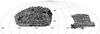 |
Fig. 1 Distribution on the sky of the SDSS-DR12/BOSS spectroscopy in J2000 equatorial coordinates (expressed in decimal degrees). |
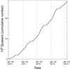 |
Fig. 2 Cumulative number of quasars as a function of observation date during the whole SDSS-III/BOSS survey. A total of 297 301 quasars was spectroscopically confirmed. The “flat portions” in this figure correspond to summer shutdowns. |
3. Construction of the DR12Q catalog
Spectra of all the SDSS-III/BOSS quasar candidates, all the SDSS-III quasar targets from ancillary programs and all the objects classified robustly as z ≥ 2 quasars by the SDSS pipeline (Bolton et al. 2012) among the galaxy targets (Reid et al. 2016) have been visually inspected. The SDSS-DR12 quasar catalog is built upon the output of the visual inspection of 546 856 such quasar candidates.
3.1. Visual inspection process
The spectra of quasar candidates are reduced by the SDSS pipeline1, which provides a classification (QSO, STAR or GALAXY) and a redshift. To achieve this, a library of stellar templates, and a principal component analysis (PCA) decomposition of galaxy and quasar spectra are fitted to each spectrum. Each class of templates is fitted in a given range of redshift: galaxies from z = −0.01 to 1.00, quasars from z = 0.0033 to 7.00, and stars from z = −0.004 to 0.004 (±1200 km s-1).
The pipeline thus provides the overall best fit (in terms of the lowest reduced χ2) and a redshift for each template and thus a classification for the object. A quality flag (ZWARNING) is associated with each measured redshift. ZWARNING = 0 indicates that the pipeline has high confidence in its estimate. This output is used as the starting point for the visual inspection process (see Bolton et al. 2012,for details).
Based on the initial SDSS pipeline classification and redshift, the quasar candidates are split into four categories: low-z (z< 2) and high-z (z ≥ 2) quasars, stars and “others”. The spectra are visually inspected through a dedicated webpage on which all spectra are matched to targeting information, imaging data and SDSS-I/II spectroscopy. The inspection is performed plate by plate for each category described above with a list of spectra whose identification and redshift can be validated at once. If an object requires a more thorough inspection, it can be inspected on a single page on which it is possible to change the redshift and identification of the object. Whenever a change of identification and/or redshift is necessary, it is done by eye. Additional flags are also set during the visual inspection when a Damped Lyman-α system or broad absorption lines (see Sect. 4.6 for further details) are seen. Finally, quality flags are set if there is an obvious reduction problem. When the redshift and identification are unambiguous based on this inspection, each object is classified QSO, Star or Galaxy and a redshift is adopted. If the pipeline redshift does not need to be modified, the SDSS pipeline redshift (Z_PIPE) and the visual inspection redshift (Z_VI) are identical. If not, the redshift is set by eye with an accuracy that cannot be better than Δz ~ 0.003. In some cases, objects undoubtedly are quasars but their redshift is uncertain; these objects are classified as QSO_Z? or QSO_BAL_Z? when the spectrum exhibits strong broad absorption lines. When the object identification is unsure they are classified either as QSO_? or as Star_?. For spectra with a moderate S/N but with a highly uncertain identification, the object is classified as ?. Finally, when the S/N is too low or the spectrum is affected by poor sky subtraction or has portions missing needed that prevent an identification, it is classified as Bad. The distinction between Bad and ? becomes somewhat subjective as the S/N decreases. Examples of spectra to illustrate these categories are shown in Fig. 3.
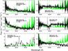 |
Fig. 3 Examples of spectra identified as QSO_? (top left), QSO_Z? (middle left), QSO_BAL_Z? (bottom left), Star_? (top right), ? (middle right), and Bad (bottom right). The fluxes are shown in black and associated errors in green. All the spectra are smoothed over 10 pixels. |
Most of the quasars are observed as part of the main SDSS-III/BOSS quasar survey whose target selection is described in Ross et al. (2012) or ancillary programs targeting quasars. In addition, we also included serendipitous quasars that were found among galaxy targets. Because these latter spectra have usually low S/N, their exact identification is more difficult. Thus, specifically for these objects we adopted a binary visual inspection classification: either an object is a QSO or is not_a_QSO.
3.2. Definition of the DR12Q parent sample
We selected objects for visual inspection from among the following targets:
-
quasar targets from the main SDSS-III/BOSS quasar survey:these targets can be identified with the BOSS_TARGET1 targetselection flag (see Rosset al. 2012, for more details);
-
ancillary programs that target quasars: these can be identified with the ANCILLARY_TARGET1 and ANCILLARY_TARGET2 target selection flags that are fully described in Appendix B of Dawson et al. (2013) and Appendix A of Alam et al. (2015);
-
quasar targets from the SDSS-IV pilot survey that can be identified with the EBOSS_TARGET0 flag. The meaning of each value of this target selection bit is fully described in Appendix A of Alam et al. (2015);
-
SDSS-III/BOSS galaxy targets that are identified by the pipeline as either QSO with z > 2 and ZWARNING set to 0, or GALAXY with the subclass BROADLINE.
These criteria led to a superset containing 546 856 objects among which we identified 297 301 QSO, 1623 QSO_?, 1490 QSO_Z?, 22 804 Galaxy, 205 282 Star, 2640 Star_?, 6292 Bad, and 2386 ?. Among the galaxy targets, 6844 objects were identified as not a QSO after their visual inspection. Finally, a total of 192 quasar targets could not be visually inspected due to bad photometric information. The identification or redshift of 53 413 objects (out of 546 856) changed with respect to the SDSS pipeline (Bolton et al. 2012). A total of 83% of objects classified by the SDSS pipeline have ZWARNING = 0, i.e. their identification and redshift are considered secure. Among this subset, the identification or redshift of 3.3% of the objects changed after visual inspection. In such a case, the redshift is adjusted by eye. For the remaining 96.7%, we kept the SDSS pipeline redshift (and associated error) and identification. Emission-line confusions are the main source of catastrophic redshift failures, and wrong identifications mostly affect stars that are confused with z ~ 1 quasars because of poor sky subtraction at the red end of their spectra. The remaining 17% of the overall sample have ZWARNING> 0, i.e. the pipeline output may not be reliable. For these objects, 41.1% of the identification or redshift changed after inspection, following the same procedure as previously. The result of the visual inspection is summarized in Table 1. The SDSS-DR12 quasar catalog lists all the firmly confirmed quasars, i.e. those identified as QSO and QSO_BAL.
Number of objects identified as such by the pipeline with any ZWARNING value (second column) and with ZWARNING = 0 (third column), and after the visual inspection (fourth column).
Together with the quasar catalog, the full result of the visual inspection, i.e. the identification of all visually inspected objects, is made available as part of the superset file from which we derive this catalog. The identification of each object described in Sect. 3.1 (e.g. QSO, QSO_Z?, Bad) is encoded with two parameters in the superset file: CLASS_PERSON and Z_CONF_PERSON. The former refers to the classification itself, QSO, Star or Galaxy, while the latter refers to our level of confidence for the redshift we associate to each object. The relation between these two parameters and the identification from Sect. 3.1 is given in Table 2. We refer the reader to Appendix B for the detailed format of the DR12 superset file, which is provided in FITS format (Wells et al. 1981).
 |
Fig. 4 Left panel: redshift distribution of the SDSS-DR12 (thick black histogram), SDSS-DR10 (orange histogram) and SDSS-DR7 (blue histogram) quasars over the redshift range 0–6. Right panel: redshift distribution of the SDSS-DR12 quasars for the CORE sample (dark blue histogram), BONUS sample (light blue histogram), ancillary programs (red histogram) and SEQUELS (orange histogram). The bin size of all the histograms is Δz = 0.05. The two peaks at z ~ 0.8 and z ~ 1.6 seen in the redshift distribution of the SDSS-DR10 and SDSS-DR12 quasar samples (left panel) and in the distribution of the CORE and BONUS samples (right panel) are due to known degeneracies in the quasar target selection (see Ross et al. 2012,for details). |
4. Summary of the sample
4.1. Broad view
The DR12Q catalog contains a total of 297 301 unique quasars, among which 184 101 have z> 2.15. This represents an increase of 78% compared to the full SDSS-DR10 quasar catalog (Pâris et al. 2014), and 121 923 quasars are new discoveries compared to the previous release. The full SDSS-III spectroscopic survey covers a total footprint of 9376 deg2, leading to an average surface density of z> 2.15 quasars of 19.64 deg-2. A total of 222 329 quasars, 167 007 having z> 2.15, are located in the SDSS-III/BOSS main quasar survey and are targeted as described in Ross et al. (2012)2. Additional BOSS-related programs3 targeted 54 639 quasars, and SEQUELS4 targeted a total of 20 333 confirmed quasars.
SDSS-DR12 quasars have redshifts between z = 0.041 and z = 6.440. The highest redshift quasar in our sample was discovered by Fan et al. (2001)5. The redshift distribution of the entire sample is shown in Fig. 4 (left panel; black histogram) and compared to the SDSS-DR7 (Schneider et al. 2010,blue histogram) and the SDSS-DR10 (Pâris et al. 2014,orange histogram) quasar catalogs. The two peaks at z ~ 0.8 and z ~ 1.6 seen in the SDSS-DR10 and SDSS-DR12 redshift distributions are due to known degeneracies in the SDSS color space. The right panel of Fig. 4 presents the redshift distribution for each main subsample: the CORE sample (dark blue histogram) designed for quasar demographics and physics studies, the BONUS sample (light blue histogram) whose goal is to maximize the number of 2.15 ≤ z ≤ 3.5 quasars, quasars observed as part of ancillary programs (red histogram) and the SDSS-IV pilot survey, i.e. the SEQUELS sample (orange histogram).
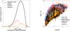 |
Fig. 5 Left panel: distribution of r PSF magnitude (corrected for Galactic extinction) for the BOSS main sample (selected by the algorithms described in Ross et al. 2012,thick black histogram), ancillary programs (red histogram) and SEQUELS (orange histogram). The bin size is Δr = 0.02. Right panel: absolute magnitude-redshift plane for SDSS-DR12 CORE+BONUS quasars (black contours), quasars observed as part of SDSS-DR12 ancillary programs (red points), SEQUELS quasars (orange points) and SDSS-DR7 quasars (blue contours). The absolute magnitudes assume H0 = 70 km s-1 Mpc-1 and the K-correction is given by Richards et al. (2006), who define K(z = 2) = 0. Contours are drawn at constant point density. |
The main SDSS-III/BOSS quasar survey is designed to target quasars in the redshift range 2.15 ≤ z ≤ 3.5 down to g = 22 or r = 21.85. The r-band magnitude (corrected for Galactic extinction) distribution of those quasars is displayed in Fig. 5 (left panel, black histogram). Each ancillary program has its own target selection (see e.g., Alam et al. 2015), leading to an extremely heterogeneous sample whose r-band PSF magnitude distribution is also shown in Fig. 5 (left panel, red histogram). Lastly, the SDSS-IV pilot survey (SEQUELS) focuses on quasars with 0.9 ≤ z ≤ 3.5 down to g = 22 or r = 22 (Myers et al. 2015). The r-band PSF magnitude distribution of the resulting sample is displayed in Fig. 5 (left panel, orange histogram). The right panel of Fig. 5 presents the luminosity-redshift plane for the three subsamples contributing to the present catalog: the SDSS-III/BOSS main survey (black contours), quasars observed as part of ancillary programs (red points) and SEQUELS quasars (orange points). The SDSS-DR7 quasars are plotted for reference in the same plane (blue contours). Typical quasar spectra are shown in Fig. 6.
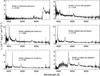 |
Fig. 6 Spectrum of the highest redshift (z = 6.440) quasar observed by BOSS is displayed in the top left panel. This quasar was discovered by Fan et al. (2001). Typical spectra of SEQUELS quasars are presented at five different redshifts: z ~ 1.2 (top right panel) and z ~ 1.6 (middle left panel). Typical BOSS quasars are shown at three different redshifts: z ~ 2.2 (middle right panel), z ~ 2.7 (bottom left panel) and z ~ 3.5 (bottom right panel). All the spectra are smoothed over 5 pixels. |
4.2. Known quasars from SDSS-I/II re-observed by SDSS-III/BOSS
As explained in Sect. 2.2, a significant fraction of known quasars from DR7Q have been re-observed by the SDSS-III/BOSS survey. The main quasar target selection (Ross et al. 2012) systematically re-targeted DR7Q quasars with zDR7 ≥ 2.15 over the entire survey. Starting from Year 3, DR7Q quasars with 1.8 ≤ zDR7< 2.15 were also re-observed with the BOSS spectrograph. Other DR7Q quasars, mostly at lower redshifts, were targeted as part of SDSS-III ancillary programs. SDSS-III/BOSS spectra were obtained for 25 416 objects listed in DR7Q. A total of 25 275 quasars known from DR7Q are included in the present catalog, i.e. are classified as QSO or QSO_BAL. A total of 59 are not part of the DR12Q catalog due to a lower confidence level of their redshift estimate, i.e., they were classified as QSO_Z? or QSO_BAL_Z?, and their current identification is included in the DR12 superset file. A total of 14 quasars dropped out of the DR12Q catalog due to bad photometric information and were not visually inspected, and 67 quasars have bad spectra, mostly “empty spectra”, in SDSS-III/BOSS. Our visual inspection is based on SDSS-III/BOSS spectroscopy only and thus, those spectra were re-classified as Bad. Finally, one object, SDSS J015957.64+003310.5, had its identification changed and was reported to be a “changing-look quasar” (LaMassa et al. 2015; Merloni et al. 2015).
The DR7Q catalog contains 19 132 quasars with z ≥ 2.15. In principle, all of these objects should have been re-observed by SDSS-III/BOSS. However, 2265 DR7Q quasars lie outside of the SDSS-III/BOSS footprint and hence were not re-targeted. The other 16 867 quasars have a SDSS-III/BOSS spectrum. Since the systematic re-observation of DR7Q quasars with 1.8 ≤ z < 2.15 started in Year 3, the completeness for those objects is much lower, with a total of 5676 having a SDSS-III/BOSS spectrum (out of 15 432 DR7Q quasars in the same redshift range).
4.3. Differences between the SDSS-DR10 and SDSS-DR12 quasar catalogs
The previous SDSS quasar catalog (DR10Q; Pâris et al. 2014) contained 166 583 quasars, 166 520 are included in the DR12Q catalog. Among the 63 “missing” quasars, 60 were identified in the galaxy targets and are now part of the supplementary list (see Sect. 6). As explained in Sect. 3.2, we define our parent sample based on quasar candidates from either the main SDSS-III/BOSS survey or ancillary programs, and we also search for serendipitous quasars among galaxy targets based on the SDSS pipeline identification. The latter definition depends on the SDSS pipeline version, leading to slight variations between parent samples drawn for each data release. However, we keep track of firm identifications from previous pipeline versions and provide them in the supplementary list.
The identification of two objects reported as quasars in DR10Q changed: one is now classified as QSO_? and the second one as Bad. Those two objects are part of the DR12Q superset with their new identification. Finally, one actual quasar (SDSS J013918.06+224128.7) dropped out of the main catalog but is part of the supplementary list. This quasar was re-observed as an emission line galaxy (ELG) candidate. The target selection bits for the two spectra are inconsistent. The best spectrum as identified by the SDSS pipeline, i.e. having SPECPRIMARY = 1, is associated with the ELG target, but not with the quasar target. It is therefore not selected to be part of our parent sample.
4.4. Uniform sample
As in DR9Q and DR10Q, we provide a uniform flag (row #31 of Table C.1) in order to identify a homogeneously selected sample of quasars. The CORE sample has been designed to have a well understood and reproducible selection function. However, its definition varied over the first year of the survey. Regions of the sky within which all the algorithms used in the quasar target selection are uniform are called “Chunks”; their definition is given in Ross et al. (2012). After Chunk 12, CORE targets were selected with the XDQSO technique only (Bovy et al. 2011). These objects have uniform = 1. Quasars in the DR12Q catalog with uniform = 2 are objects that would have been selected by XDQSO if it had been the CORE algorithm prior to Chunk 12. Objects with uniform = 2 are reasonably complete to what XDQSO would have selected, even prior to Chunk 12. DR12Q only contains information about spectroscopically confirmed quasars and not about all targets. Hence, care must be taken to draw a statistical sample from the uniform flag. See, e.g., the discussion regarding the creation of a statistical sample for clustering measurements in White et al. (2012) and Eftekharzadeh et al. (2015). Quasars with uniform = 0 are not homogeneously selected CORE targets.
4.5. Accuracy of redshift estimates
The present catalog contains six different redshift estimates: the visual inspection redshift (Z_VI), the SDSS pipeline redshift (Z_PIPE), a refined PCA redshift (Z_PCA) and three emission-line based redshifts (Z_CIV, Z_CIII and Z_MGII).
As described in Sect. 3.1, quasar redshifts provided by the SDSS pipeline (Bolton et al. 2012) are the result of a linear combination of four eigenspectra. The latter were derived from a principal component analysis (PCA) of a sample of quasars with robust redshifts. Hence, this does not guarantee this value to be the most accurate (e.g. Hewett & Wild 2010; Shen et al. 2016). The SDSS pipeline has a very high success rate in terms of identification and redshift estimate, and in order to correct for the remaining misidentifications and catastrophic redshift failures, we perform the systematic visual inspection of all quasar targets. In case we modified the SDSS pipeline redshift, the visual inspection redshift provides a robust value, set to be at the location of the maximum of the Mg ii emission line, when this emission line is available in the spectrum. The estimated accuracy is Δz = 0.003. This value corresponds to the limit below which we are no longer able to see any difference by eye.
We also provide a homogeneous automated redshift estimate (Z_PCA) that is based on the result of a PCA performed on a sample of quasars with redshifts measured at the location of the maximum of the Mg ii emission line (see Pâris et al. 2012,for details). The Mg ii line is chosen as the reference because this is the broad emission line the least affected by systematic shifts with respect to the systemic redshift (e.g. Hewett & Wild 2010; Shen et al. 2016). In addition to this PCA redshift, we also provide the redshift corresponding to the position of the maximum of the three broad emission lines we fit as part of this catalog: C ivλ1550, C iii]λ1909 and Mg iiλ2800.
Hewett & Wild (2010) carefully studied the systematic emission-lines shifts in the DR6 quasar sample and computed accurate quasar redshifts by correcting for these shifts. In DR12Q, there are 5328 non-BAL quasars that have redshifts measured by Hewett & Wild (2010) available and for which we also have Mg ii redshifts that are expected to be the closest estimates to the quasar systemic redshift. Mg ii-based redshifts are redshifted by 3.3 km s-1 compared to the Hewett & Wild (2010) measurements, with a dispersion of 326 km s-1. This confirms that Mg ii redshifts provide a reliable and accurate measurement.
80 791 have the six redshift measurements provided in our catalog available. We compute the redshift difference, expressed as velocities, for Z_VI, Z_MGII, Z_PIPE, Z_CIV and Z_CIII with respect to Z_PCA. We take the latter as our reference because this measurement is uniformally run over the entire DR12Q sample. The distributions of redshift differences are shown in Fig. 7. Mg ii-based redshifts are redshifted by 2.1 km s-1 compared to the PCA redshifts with a dispersion of 680 km s-1. In average, visual inspection redshifts are blueshifted by 15.3 km s-1 with respect to the PCA redshifts with a dispersion of 529 km s-1. The SDSS pipeline estimates are redshifted by 42.7 km s-1 with a dispersion of 637 km s-1. Finally, as expected, C iv and C iii] redshifts are the most shifted with respect to the PCA redshifts with an average blueshift of 321 km s-1 and 312 km s-1 respectively.
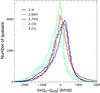 |
Fig. 7 Distribution of velocity differences between the visual inspection redshift (Z_VI, black histogram), Mg ii-based redshift (Z_MGII, red histogram), SDSS pipeline redshift (Bolton et al. 2012,blue histogram), C iv-based redshift (Z_CIV, green histogram), C iii]-based redshift (Z_CIII, cyan histogram) and the PCA redshift (Z_PCA). The bin size of all the histograms is Δv = 50 km s-1. |
4.6. Broad Absorption Line quasars
As described in Pâris et al. (2012), quasars displaying broad absorption lines (BAL) are flagged in the course of the visual inspection of all the quasar targets. This flag (BAL_FLAG_VI, Col. #56 of Table C.1) provides qualitative information about the existence of such features only. We refer the reader to Sect. 5 of Pâris et al. (2012) for a full discussion of the robustness of the visual inspection detection of BALs. A total of 29 580 quasars have been flagged in the course of visual inspection.
In order to have a more systematic detection of BALs and quantitative measurement of their properties, we automatically search for BAL features and report metrics of common use in the community: the BALnicity index (BI; Weymann et al. 1991) and the absorption index (AI; Hall et al. 2002) of the C iv absorption troughs. We restrict the automatic search to quasars with Z_VI≥ 1.57 in order to have the full spectral coverage of C iv absorption troughs.
The BALnicity index (Col. #57) is computed bluewards of the C iv emission line and is defined as: ![\begin{equation} {\rm BI} ~=~ - \int ^{3000} _{25000} \left[ 1 - \frac{f \left( v \right)}{0.9} \right] C \left( v \right) {\rm d}v , \label{eq:BI_def} \end{equation}](/articles/aa/full_html/2017/01/aa27999-15/aa27999-15-eq108.png) (1)where
(1)where  is the normalized flux density as a function of velocity displacement from the emission-line center. The quasar continuum is estimated using a linear combination of four principal components as described in Pâris et al. (2012).
  is initially set to 0 and can take only two values, 1 or 0. It is set to 1 whenever the quantity
  is continuously positive over an interval of at least 2000 km s-1. It is reset to 0 whenever this quantity becomes negative. C iv absorption troughs wider than 2000 km s-1 are detected in the spectra of 16 442 quasars. The number of lines of sight in which BI_CIV is positive is lower than the number of visually flagged BAL for several reasons: (i) the visual inspection provides a qualitative flag for absorption troughs that do not necessarily meet the requirements defined in Eq. (1); (ii) the visual inspection is not restricted to any search window; and (iii) the visual inspection flags rely on absorption troughs due to other species in addition to C iv (especially Mg ii). The distribution of BI for C iv troughs from DR12Q is plotted in the right panel of Fig. 8 (black histogram) and is compared to previous works by Gibson et al. (2009, blue histogram) performed on DR5Q (Schneider et al. 2007) and by Allen et al. (2011, red histogram) who searched for BAL quasars in quasar spectra released as part of SDSS-DR6 (Adelman-McCarthy et al. 2008). The three distributions are normalized.
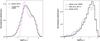 |
Fig. 8 Left panel: distribution of AI for the SDSS-DR3 (magenta histogram; Trump et al. 2006) and the SDSS-DR12 (black histogram) quasars. Both distributions are normalized to have a surface area equal to 1 for log AI > 2.5. Right panel: distribution of BI from the DR12Q catalog (black histogram), from the SDSS-DR6 (red histogram; Allen et al. 2011) and from the SDSS-DR5 (blue histogram; Gibson et al. 2009). All the distributions are normalized to have their sum equal to 1. |
The overall shapes of the three distributions are similar. The BI distribution from Gibson et al. (2009) exhibits an excess of low-BI values compared to Allen et al. (2011) and this work. The most likely explanation is the difference in the quasar emission modeling. Allen et al. (2011) used a non-negative matrix factorization (NMF) to estimate the unabsorbed flux, which produces a quasar emission line shape akin to the one we obtain with PCA. Gibson et al. (2009) modeled the quasar continuum with a reddened power-law and strong emission lines with Voigt profiles. Power-law like continua tend to underestimate the actual quasar emission and hence, the resulting BI values tend to be lower than the one computed when the quasar emission is modeled with NMF or PCA methods.
For weaker absorption troughs, we compute the absorption index (Col. #59) as defined by Hall et al. (2002): ![\begin{equation} {\rm AI} ~=~ - \int ^{0} _{25000} \left[ 1 - \frac{f \left( v \right)}{0.9} \right] C \left( v \right) {\rm d}v , \label{eq:AI_def} \end{equation}](/articles/aa/full_html/2017/01/aa27999-15/aa27999-15-eq113.png) (2)where is the normalized continuum and has the same definition as in Eq. (1)except that the threshold to set C to 1 is reduced to 450 km s-1. Following Trump et al. (2006), we calculate the reduced χ2 for each trough, i.e. where C = 1:
(2)where is the normalized continuum and has the same definition as in Eq. (1)except that the threshold to set C to 1 is reduced to 450 km s-1. Following Trump et al. (2006), we calculate the reduced χ2 for each trough, i.e. where C = 1: 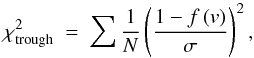 (3)where N is the number of pixels in the trough, is the normalized flux and σ the estimated rms noise for each pixel. The greater the value of
  , the more likely the trough is not due to noise. Following the recommendations of Trump et al. (2006), we report AIs when at least one C iv absorption trough is detected with
  . A total of 48 863 quasars satisfy this definition. The distribution of AI with is shown in the left panel of Fig. 8 (black histogram) and is compared to the results of Trump et al. (2006, magenta histogram). Both distributions are normalized to have a surface area equal to 1 for log AI > 2.5. The distributions are similar. The main difference between the two distributions is the existence of a tail at low AI in DR12Q. This is due to the modified definition for AI used in Trump et al. (2006): the 0.9 factor in Eq. (2)was removed and the detection threshold was larger (1000 km s-1 instead of 450 km s-1 here).
We also report the number of troughs detected with widths larger than 2000 km s-1 (Col. #62 in Table C.1) and larger than 450 km s-1 (Col. #65) together with the velocity ranges over which these troughs are detected (Cols. #63-64 and #66-67, respectively).
Format of the binary FITS file that contains “trough-by-trough” information for BAL quasars.
BAL information reported in the DR12Q catalog is computed over all the absorption troughs that are detected. However, out of 29 580 quasars with BAL_FLAG_VI = 1, i.e. flagged during the visual inspection process, 16 693 have more than one absorption trough larger than 450 km s-1 detected in the spectrum (out of 21 444 with AI > 0), and 2564 with more than one absorption trough larger than 2000 km s-1 (out of 15 044 with BI > 0). We provide detailed “trough-by-trough” information for all BAL_FLAG_VI = 1 quasars in a separate file whose format is described in Table 3. For each detected absorption trough, we measure the velocity range in which the normalized flux density6 is measured to be lower than 0.9, given the position of its minimum and the value of the normalized flux density at this location.
4.7. Multi-wavelength cross-correlation
We provide multi-wavelength matching of DR12Q quasars to several surveys: the FIRST radio survey (Becker et al. 1995), the Galaxy Evolution Explorer (GALEX, Martin et al. 2005) survey in the UV, the Two Micron All Sky Survey (2MASS, Cutri et al. 2003; Skrutskie et al. 2006), the UKIRT Infrared Deep Sky Survey (UKIDSS; Lawrence et al. 2007), the Wide-Field Infrared Survey (WISE, Wright et al. 2010), the ROSAT All-Sky Survey (RASS; Voges et al. 1999, 2000), and the fourth data release of the Third XMM-Newton Serendipitous Source Catalog (Watson et al. 2009).
4.7.1. FIRST
As for the previous SDSS-III/BOSS quasar catalogs, we matched the DR12Q quasars to the latest FIRST catalog (March 2014; Becker et al. 1995) using a 2′′ matching radius. We report the flux peak density at 20 cm and the signal-to-noise ratio of the detection. Among the DR12Q quasars, 29 671 lie outside of the FIRST footprint and have their FIRST_MATCHED flag set to −1.
The SDSS-III/BOSS quasar target selection (Ross et al. 2012) automatically includes matches to the FIRST sources from a previous (July 2008) version of the FIRST catalog that have (u−g) > 0.4. This additional color cut is set to avoid contamination by low-redshift quasars.
A total of 10 221 quasars have FIRST counterparts in DR12Q. We estimate the fraction of chance superposition by offsetting the declination of DR12Q quasars by 200′′. We then re-match to the FIRST source catalog. We conclude that there are about 0.2% of false positives in the DR12Q-FIRST matching.
4.7.2. The Galaxy Evolution Explorer (GALEX)
As for DR10Q, GALEX (Martin et al. 2005) images are force-photometered (from GALEX Data Release 5) at the SDSS-DR8 centroids (Aihara et al. 2011), such that low S/N point-spread function fluxes of objects not detected by GALEX are recovered, for both the FUV (1350–1750 Å) and NUV (1750–2750 Å) bands when available. A total of 197 781 quasars are detected in the NUV band, 158 474 in the FUV band and 129 090 have non-zero fluxes in both bands.
4.7.3. The Two Micron All Sky Survey (2MASS)
We cross-correlate DR12Q with the All-Sky Data Release Point Source catalog (Skrutskie et al. 2006) using a matching radius of 2′′. We report the Vega-based magnitudes in the J, H and K-bands and their error together with the signal-to-noise ratio of the detections. We also provide the value of the 2MASS flag rd_flg[1], which defines the peculiar values of the magnitude and its error for each band7.
There are 471 matches in the catalog. This number is quite small compared with the number of DR12Q quasars because the sensitivity of 2MASS is much less than that of SDSS. Applying the same method as described in Sect. 4.7.1, we estimate that 0.8% of the matches are false positives.
4.7.4. The Wide-Field Infrared Survey (WISE)
Previous SDSS-III/BOSS quasar catalogs (Pâris et al. 2012, 2014) were matched to the WISE All-Sky Source catalog8 (Wright et al. 2010). For this version of the quasar catalog, we matched the DR12Q to the newly released AllWISE Source Catalog9 (Wright et al. 2010; Mainzer et al. 2011) that has enhanced photometric sensitivity and accuracy, and improved astrometric precision. Our procedure is the same as in DR9Q and DR10Q, with a matching radius of 2.0′′ which provides a low level of false positive matches (see e.g. Fig. 4 of Krawczyk et al. 2013). There are 190 408 matches from the AllWISE Source Catalog. Following the procedure described in Sect. 4.7.1, we estimate the rate of false positive matches to be about 2%.
We report the magnitudes, their associated errors, the S/N of the detection and reduced χ2 of the profile-fitting in the four WISE bands centered at wavelengths of 3.4, 4.6, 12 and 22 μm. These magnitudes are in the Vega system, and are measured with profile-fitting photometry. We also report the WISE catalog contamination and confusion flag, cc_flags, and their photometric quality flag, ph_qual. As suggested on the WISE “Cautionary Notes” page10, we recommend using only those matches with cc_flags = “0000” to exclude objects that are flagged as spurious detections of image artifacts in any band. Full details about quantities provided in the AllWISE Source Catalog can be found on their online documentation11.
4.7.5. UKIDSS
As for DR10Q, near infrared images from the UKIRT Infrared Deep Sky Survey (UKIDSS; Lawrence et al. 2007) are force-photometered at the SDSS-DR8 centroids (Aihara et al. 2011).
We provide the fluxes and their associated errors, expressed in W m-2 Hz-1, in the Y, J, H and K bands. The conversion to the Vega magnitudes, as used in 2MASS, is given by the formula:  (4)where X denotes the filter and the zero-point values f0,X are 2026, 1530, 1019 and 631 for the Y, J, H and K bands respectively.
A total of 78 783 quasars are detected in at least one of the four bands Y, J, H or K. 78 079 objects are detected in the Y band, 77 761 in the J band, 77 726 in H band, 78 179 in the K band and 75 987 objects have non-zero fluxes in the four bands. Objects with zero fluxes lie outside the UKIDSS footprint. The UKIDSS limiting magnitude is K ~ 18 (for the Large Area Survey) while the 2MASS limiting magnitude in the same band is ~15.3. This difference in depth between the two surveys explains the large difference in the numbers of matches with DR12Q.
4.7.6. ROSAT all sky survey
As we did for the previous SDSS-III/BOSS quasar catalogs, we matched the DR12Q quasars to the ROSAT all sky survey Faint (Voges et al. 2000) and Bright (Voges et al. 1999) source catalogues with a matching radius of 30′′. Only the most reliable detections are included in our catalog: when the quality detection is flagged as potentially problematic, we do not include the match. A total of 1463 quasars are detected in one of the RASS catalogs. As for the cross-correlations described above, we estimate that 2.1% of the RASS-DR12Q matches are due to chance superposition.
4.7.7. XMM-Newton
DR12Q was cross-correlated with the fourth data release of the Third XMM-Newton Serendipitous Source Catalog12 (3XMM-DR4) using a standard 5.0′′ matching radius. The 3XMM-DR4 catalog benefits from an increase of the number of public observations leading to an increase of ~40% of the number of unique sources. Furthermore, significant improvements of the XMM-Newton science analysis software and calibration allow the detection of fainter sources. Thanks to these changes in the XMM-Newton Serendipitous Source Catalog, the overall number of matches increased by ~50%. For each of the 5354 DR12Q quasars with XMM-Newton counterparts, we report the total flux (0.2–12 keV), and associated error, from the three XMM-Newton CCDs (MOS1, MOS2, PN). In the case of multiple XMM-Newton observations, the one with the longest exposure time was used to compute the total flux. We also report the soft (0.2–2 keV), hard (4.5–12 keV) and total (0.2–12 keV) fluxes, and associated errors, that were computed as the weighted average of all the detections in the three cameras. Corresponding observed X-ray luminosities are computed in each band and are not absorption corrected. All fluxes and errors are expressed in erg cm-2 s-1 and luminosities are computed using the visual inspection redshift (Z_VI). Finally, in the case of no detection or detection with significant errors (less than 1σ detections), we provide an upper limit for the flux in the hard band (2–10 keV). Such sources have the flag LX2_10_UPPER set to −1.
4.8. Variability
Photometric variability has proven to be an efficient method to distinguish quasars from stars even in redshift ranges where their colors overlap (e.g. Palanque-Delabrouille et al. 2011, 2013; Peters et al. 2015). The variability of astronomical sources can be characterized by their “structure function” that is a measurement of the amplitude of the observed variability as a function of the time delay between two observations (e.g. Schmidt et al. 2010). This function is modeled as a power-law parametrized in terms of A, the mean amplitude of the variation on a one-year timescale (in the observer’s reference frame) and γ, the logarithmic slope of the variation amplitude with respect to time. With Δmij defined as the difference between the magnitudes of the source at time ti and tj, and assuming an underlying Gaussian distribution of Δm values, the model predicts an evolution of the variance σ2(Δm) with time according to ![\begin{equation} \sigma ^2 \left( \Delta m \right) ~=~ \left[ A \left( \Delta t_{ij} \right) ^{\gamma} \right] ^2 + \left( \sigma ^2 _i + \sigma ^2 _j \right), \label{eq:str_func} \end{equation}](/articles/aa/full_html/2017/01/aa27999-15/aa27999-15-eq141.png) (5)where σi and σj are the photometric errors at time ti and tj. Quasars are expected to lie at high A and γ, non-variable stars to lie near A = γ = 0 and variable stars to have γ ~ 0 even if A can be large. In addition, variable sources are expected to deviate greatly in a χ2 sense from a model with constant flux.
(5)where σi and σj are the photometric errors at time ti and tj. Quasars are expected to lie at high A and γ, non-variable stars to lie near A = γ = 0 and variable stars to have γ ~ 0 even if A can be large. In addition, variable sources are expected to deviate greatly in a χ2 sense from a model with constant flux.
DR12Q quasars lying in the Stripe 82 region, i.e. with 300° <αJ2000 < 360° or 0° <αJ2000 < 50° and −1.25° <δJ2000 < +1.25°, have typically 60 epochs of imaging reported in DR9 (Ahn et al. 2012). In the rest of the SDSS-III/BOSS footprint, photometric data from SDSS-DR9 (Ahn et al. 2012) and the Palomar Transient Factory (PTF; Rau et al. 2009; Law et al. 2009) were combined to construct light curves, providing between 3 and 10 epochs. A “PTF epoch” in this context actually corresponds to coadded imaging data from a few tens of single-epoch PTF images, up to a thousand in the case of some frequently observed PTF fields. The duration of one “PTF epoch” ranges from several months to one year. Combined PTF+SDSS light curves, and the variability related observables, are consistently measured in the PTF R-band filter, which is related to SDSS photometric system by R ≃ r + α(r−i) with α = 0.20–0.22 (Ofek et al. 2012).
As part of DR12Q, we provide the structure function parameters A (VAR_A) and γ (VAR_GAMMA) as defined in Eq. (5)for each object with variability data. We also give the reduced χ2 (VAR_CHI2) when each light curve is fitted with a constant, i.e., when no variability is assumed. The value of the VAR_MATCHED flag is the number of photometric epochs used to estimate the quasar variability. A total of 143 359 quasars have variability data available. When no variability information is available, this flag is set to 0.
5. Description of the DR12Q catalog
The DR12Q catalog is available as a binary FITS table file at the SDSS public website13. All the required documentation (format, name, unit of each column) is provided in the FITS header, and it is also summarized in Table C.1.
Notes on the catalog columns:
-
1.
The DR12 object designation, given by the formatSDSS Jhhmmss.ss+ddmmss.s; only the final 18 characters arelisted in the catalog (i.e., the character string“SDSS J”is dropped). The coordinates in theobject name follow IAU convention and are truncated, notrounded.
-
2–3.
The J2000 coordinates (Right Ascension and Declination) in decimal degrees. The astrometry is from SDSS-DR12 (Alam et al. 2015).
-
4.
The 64-bit integer that uniquely describes the objects that are listed in the SDSS (photometric and spectroscopic) catalogs (THING_ID).
-
5–7.
Information about the spectroscopic observation (Spectroscopic plate number, Modified Julian Date, and spectroscopic fiber number) used to determine the characteristics of the spectrum. These three numbers are unique for each spectrum, and can be used to retrieve the digital spectra from the public SDSS database. When an object has been observed more than once, we selected the best quality spectrum as defined by the SDSS pipeline (Bolton et al. 2012), i.e. with SPECPRIMARY = 1.
-
8.
Redshift from the visual inspection, Z_VI.
-
9.
Redshift from the BOSS pipeline (Bolton et al. 2012).
-
10.
Error on the BOSS pipeline redshift estimate.
-
11.
ZWARNING flag from the pipeline. ZWARNING > 0 indicates uncertain results in the redshift-fitting code (Bolton et al. 2012).
-
12.
Automatic redshift estimate using a linear combination of four principal components (see Sect. 4 of Pâris et al. 2012,for details). When the velocity difference between the automatic PCA and visual inspection redshift estimates is larger than 5000 km s-1, this PCA redshift is set to −1.
-
13.
Error on the automatic PCA redshift estimate. If the PCA redshift is set to −1, the associated error is also set to −1.
-
14.
Estimator of the PCA continuum quality (between 0 and 1) as given in Eq. (11) of Pâris et al. (2011).
-
15–17.
Redshifts measured from the C iv, the C iii] complex and the Mg ii emission lines from a linear combination of five principal components (see Pâris et al. 2012). The line redshift is estimated using the position of the maximum of each emission line, contrary to Z_PCA (column #12) which is a global estimate using all the information available in a given spectrum.
-
18.
Morphological information: objects classified as a point source by the SDSS photometric pipeline have SDSS_MORPHO = 0 while extended quasars have SDSS_MORPHO = 1. The vast majority of the quasars included in the present catalog are unresolved (SDSS_MORPHO = 0) as this is a requirement of the main quasar target selection (Ross et al. 2012).
-
19–22.
The main target selection information is tracked with the BOSS_TARGET1 flag bits (19; see Table 2 in Ross et al. 2012,for a full description). Ancillary program target selection is tracked with the ANCILLARY_TARGET1 (20) and ANCILLARY_ TARGET2 (21) flag bits. The bit values and the corresponding program names are listed in Dawson et al. (2013), Alam et al. (2015), and Appendix B of this paper. The SEQUELS program targeted different classes of objects (quasars, LRG, galaxy clusters). All the SEQUELS targets are identified by the ANCILLARY_TARGET2 bit 53, and the details of each target class is provided through the EBOSS_TARGET0 flag (Col. #22; see Table A.1).
-
23–26.
If a quasar in DR12Q was observed more than once during the survey, the number of additional SDSS-III/BOSS spectra is given by NSPEC_BOSS (Col. #23). The associated plate (PLATE_DUPLICATE), MJD (MJD_DUPLICATE) and fiber (FIBERID_DUPLICATE) numbers are given in Cols. #24, 25 and 26 respectively. If a quasar was observed N times in total, the best spectrum is identified in Cols. #5–7, the corresponding NSPEC_BOSS is N-1, and the first N-1 columns of PLATE_DUPLICATE, MJD_DUPLICATE and FIBERID_DUPLICATE are filled with relevant information. Remaining columns are set to −1.
-
27.
A quasar previously known from the SDSS-DR7 quasar catalog has an entry equal to 1, and 0 otherwise. During Year 1 and 2, most SDSS-DR7 quasars with z ≥ 2.15 were re-observed. After Year 2, SDSS-DR7 quasars with z ≥ 1.8 were systematically re-observed.
-
28–30.
Spectroscopic plate number, Modified Julian Date, and spectroscopic fiber number in SDSS-DR7.
-
31.
Uniform flag. See Sect. 4.4.
-
32.
Spectral index αν. The continuum is approximated by a power-law, fcont ∝ ναν, and is computed in emission line free regions: 1450–1500 Å, 1700–1850 Å and 1950–2750 Å in the quasar rest frame.
-
33.
Median signal-to-noise ratio per pixel computed over the whole spectrum for the best spectrum as defined by the SDSS pipeline, i.e., with SPECPRIMARY = 1 (Bolton et al. 2012).
-
34.
Median signal-to-noise ratio per pixel computed over the whole spectrum of quasars observed multiple times. If there is no multiple spectroscopic observation available, the S/N value is set to −1.
-
35–37.
Median signal-to-noise ratio per pixel computed over the windows 1650–1750 Å (Col. #35), 2950–3050 Å (Col. #36) and 2950–3050 Å (Col. #37) in the quasar rest frame. If the wavelength range is not covered by the BOSS spectrum, the value is set to −1.
-
38–41.
FWHM (km s-1), blue and red half widths at half-maximum (HWHM; the sum of the latter two equals FWHM), and amplitude (in units of the median rms pixel noise, see Sect. 4 of Pâris et al. 2012) of the C iv emission line. If the emission line is not in the spectrum, the red and blue HWHM and the FWHM are set to −1.
-
42–43.
Rest frame equivalent width and corresponding uncertainty in Å of the C iv emission line. If the emission line is not in the spectrum, these quantities are set to −1.
-
44–47.
Same as 38–41 for the C iii] emission complex. It is well known that C iii]λλ1909 is blended with Si iii]λλ1892 and to a lesser extent with Al iii]λλ1857. We do not attempt to deblend these lines. Therefore the redshift and red side of the HWHM derived for this blend correspond to C iii]λλ1909. The blue side of the HWHM is obviously affected by the blend.
-
48–49.
Rest frame equivalent width and corresponding uncertainty in Å of the C iii] emission complex.
-
50–53.
Same as 38–41 for the Mg ii emission line.
-
54–55.
Rest frame equivalent width and corresponding uncertainty in Å of the Mg ii emission line. We do not correct for the neighboring Fe ii emission. Note that Albareti et al. (2015) released the output of [O iii]λ4960, 5008 Å emission-line fitting for a subset of the present catalog.
-
56.
BAL flag from the visual inspection, BAL_FLAG_VI. If a BAL feature was identified in the course of the visual inspection, BAL_FLAG_VI is set to 1, the flag is set to 0 otherwise. BAL quasars are flagged during the visual inspection at any redshift and whenever a BAL feature is seen in the spectrum (not only for C iv absorption troughs).
-
57–58.
Balnicity index (BI; Weymann et al. 1991) for C iv troughs, and their errors, expressed in km s-1. See definition in Sect. 4.6. The Balnicity index is measured for quasars with z> 1.57 only, so that the trough enters into the BOSS wavelength region. If the BAL flag from the visual inspection is set to 1 and the BI is equal to 0, this means either that there is no C iv trough (but a trough is seen in another transition) or that the trough seen during the visual inspection does not meet the formal requirement of the BAL definition. In cases with poor fits to the continuum, the balnicity index and its error are set to −1.
-
59–60.
Absorption index, and its error, for C iv troughs expressed in km s-1. See definition in Sect. 4.6. In cases with a poor continuum fit, the absorption index and its error are set to −1.
-
61.
Following Trump et al. (2006), we calculate the reduced χ2 which we call
 for each C iv trough from Eq. (3). We require that troughs have
  > 10 to be considered as true troughs.
 -
62.
Number of C iv troughs of width larger than 2000 km s-1.
-
63–64.
Limits of the velocity range in which C iv troughs of width larger than 2000 km s-1 and reaching at least 10% below the continuum are to be found. Velocities are positive bluewards and the zero of the scale is at Z_VI. So if there are multiple troughs, this value demarcates the range from the first to the last trough.
-
65.
Number of troughs of width larger than 450 km s-1.
-
66–67.
Same as 63–64 for C iv troughs of width larger than 450 km s-1.
-
68–70.
Rest frame equivalent width in Å of Si iv, C iv and Al iii troughs detected in BAL quasars with BI_CIV > 500 km s-1 and SNR_1700 > 5 (See Col. #35). They are set to 0 otherwise or in cases where no trough is detected and to −1 if the continuum is not reliable.
-
71–72.
The SDSS Imaging Run number (RUN_NUMBER) and the Modified Julian Date (MJD) of the photometric observation used in the catalog (PHOTO_MJD).
-
73–76.
Additional SDSS processing information: the photometric processing rerun number (RERUN_NUMBER); the camera column (1–6) containing the image of the object (COL_NUMBER), the field number of the run containing the object (FIELD_NUMBER), and the object identification number (OBJ_ID, see Stoughton et al. 2002, for descriptions of these parameters).
-
77–78.
DR12 PSF fluxes, expressed in nanomaggies14, and inverse variances (not corrected for Galactic extinction) in the five SDSS filters.
-
79–80.
DR12 PSF AB magnitudes (Oke & Gunn 1983) and errors (not corrected for Galactic extinction) in the five SDSS filters (Lupton et al. 1999). These magnitudes are Asinh magnitudes as defined in Lupton et al. (1999).
-
81.
DR8 PSF fluxes (not corrected for Galactic extinction), expressed in nanommagies, in the five SDSS filters. This photometry is the one that was used for the main quasar target selection (Ross et al. 2012).
-
82.
The absolute magnitude in the i band at z = 2 calculated using a power-law (frequency) continuum index of −0.5. The K-correction is computed using Table 4 from Richards et al. (2006). We use the SDSS primary photometry to compute this value.
-
83.
The Δ(g−i) color, which is the difference in the Galactic extinction corrected (g−i) for the quasar and that of the mean of the quasars at that redshift. If Δ(g−i) is not defined for the quasar, which occurs for objects at either z< 0.12or z> 5.12 ; the column will contain “−9999”.
-
84.
Galactic extinction in the five SDSS bands based on the maps of Schlegel et al. (1998). The quasar target selection was done using these maps.
-
85.
Galactic extinction in the five SDSS bands based on Schlafly & Finkbeiner (2011).
-
86.
The logarithm of the Galactic neutral hydrogen column density along the line of sight to the quasar. These values were estimated via interpolation of the 21-cm data from Stark et al. (1992), using the COLDEN software provided by the Chandra X-ray Center. Errors associated with the interpolation are expected to be typically less than ≈1 × 1020 cm-2 (e.g., see Sect. 5 of Elvis et al. 1994).
-
87.
Flag for variability information. If no information is available, VAR_MATCHED is set to 0. When enough photometric epochs are available to build a lightcurve, VAR_MATCHED is equal to the number of photometric epochs used. For PTF-selected objects (EBOSS_TARGET0, bit 11), both PTF and SDSS photometry were used. For objects lying in the stripe 82 region, only SDSS photometry was used.
-
88.
Light curves were fit by a constant flux (see Sect. 2.3 in Palanque-Delabrouille et al. 2011). The reduced χ2 of this fit is provided in VAR_CHI2.
-
89–90.
The best fit values of the structure function parameters A and γ, as defined in Eq. (5), are reported in Col. 89 (VAR_A) and 90 (VAR_GAMMA), respectively.
-
91.
The logarithm of the vignetting-corrected count rate (photons s-1) in the broad energy band (0.1–2.4 keV)from the ROSAT All-Sky Survey Faint Source Catalog (Voges et al. 2000) and the ROSAT All-Sky Survey Bright Source Catalog (Voges et al. 1999). The matching radius was set to 30′′ (see Sect. 4.7.6).
-
92.
The S/N of the ROSAT measurement.
-
93.
Angular separation between the SDSS and ROSAT All-Sky Survey locations (in arcseconds).
-
94.
Number of XMM-Newton matches in a 5′′ radius around the SDSS-DR12 quasar positions.
-
95–96.
Total X-ray flux (0.2–12 keV) from the three XMM-Newton CCDs (MOS1, MOS2 and PN), expressed in erg cm-2 s-1, and its error. In the case of multiple XMM-Newton observations, only the longest exposure was used to compute the reported flux.
-
97–98.
Soft X-ray flux (0.2–2 keV) from XMM-Newton matching, expressed in erg cm-2 s-1, and its error. In the case of multiple observations, the values reported here are the weighted average of all the XMM-Newton detections in this band.
-
99–100.
Hard X-ray flux (4.5–12 keV) from XMM-Newton matching, expressed in erg cm-2 s-1, and its error. In the case of multiple observations, the values reported here are the weighted average of all the XMM-Newton detections in this band.
-
101–102.
Total X-ray flux (0.2–12 keV) from XMM-Newton matching, expressed in erg cm-2 s-1, and its error. In the case of multiple observations, the values reported here are the weighted average of all the XMM-Newton detections in this band. For single observations, the total X-ray flux reported in Col. 101 (FLUX02_12KEV) is equal to the one reported in Col. 95 (FLUX02_12KEV_SGL).
-
103.
Total X-ray luminosity (0.2–12 keV) derived from the flux computed in Col. #95, expressed in erg s-1. This value is computed using the visual inspection redshift (Z_VI) and is not absorption corrected.
-
104.
X-ray luminosity in the 0.5–2 keV band of XMM-Newton, expressed in erg s-1. This value is computed using the visual inspection redshift (Z_VI), H0 = 70 km s-1 Mpc-1, Ωm = 0.3, ΩΛ = 0.7 and is not absorption corrected.
-
105.
X-ray luminosity in the 4.5–12 keV band of XMM-Newton, expressed in erg s-1. This value is computed using the visual inspection redshift (Z_VI), H0 = 70 km s-1 Mpc-1, Ωm = 0.3, ΩΛ = 0.7 and is not absorption corrected.
-
106.
Total X-ray luminosity (0.2–12 keV) using the flux value reported in Col. 101. This value is computed using the visual inspection redshift (Z_VI), H0 = 70 km s-1 Mpc-1, Ωm = 0.3, ΩΛ = 0.7 and is not absorption corrected.
-
107.
In the case of an unreliable detection or no detection in the 2–10 keV band the flux reported in Col. 101 is an upper limit. In that case, the LUMX2_10_UPPER flag listed in this column is set to −1.
-
108.
Angular separation between the XMM-Newton and SDSS-DR12 locations, expressed in arcsec.
-
109.
If a SDSS-DR12 quasar matches with GALEX photometring, GALEX_MATCHED is set to 1, 0 if not.
-
110–113.
UV fluxes and inverse variances from GALEX, aperture-photometered from the original GALEX images in the two bands FUV and NUV. The fluxes are expressed in nanomaggies.
-
114–115.
The J magnitude and error from the Two Micron All Sky Survey All-Sky Data Release Point Source Catalog (Cutri et al. 2003) using a matching radius of 2.0′′ (see Sect. 4.7.3). A non-detection by 2MASS is indicated by a “0.000” in these columns. The 2MASS measurements are in Vega, not AB, magnitudes.
-
116–117.
Signal-to-noise ratio in the J band and corresponding 2MASS jr_d flag that gives the meaning of the peculiar values of the magnitude and its error15.
-
118–121.
Same as 114–117 for the H-band.
-
122–125.
Same as 114–117 for the K-band.
-
126.
Angular separation between the SDSS-DR12 and 2MASS positions (in arcsec).
-
127–128.
The w1 magnitude and error from the Wide-field Infrared Survey Explorer (WISE; Wright et al. 2010) AllWISE Data Release Point Source Catalog using a matching radius of 2′′.
-
129–130.
Signal-to-noise ratio and χ2 in the WISE w1 band.
-
131–134.
Same as 127–130 for the w2-band.
-
135–138.
Same as 127–130 for the w3-band.
-
139–142.
Same as 127–130 for the w4-band.
-
143.
WISE contamination and confusion flag.
-
144.
WISE photometric quality flag.
-
145.
Angular separation between SDSS-DR12 and WISE positions (in arcsec).
-
146.
If a SDSS-DR12 quasar matches UKIDSS aperture-photometering data, UKIDSS_MATCHED is set to 1, it is set to 0 if not.
-
147–154.
Flux density and error from UKIDSS, aperture-photometered from the original UKIDSS images in the four bands Y (Col. #147–148), J (Col. #149–150), H (Col. #151–152) and K (Col. #153–154). The fluxes and errors are expressed in W m-2 Hz-1.
-
155.
If there is a source in the FIRST radio catalog (version March 2014) within 2.0′′ of the quasar position, the FIRST_MATCHED flag provided in this column is set to 1, 0 if not. If the quasar lies outside of the FIRST footprint, it is set to −1.
-
156.
This column contains the FIRST peak flux density, expressed in mJy.
-
157.
The signal-to-noise ratio of the FIRST source whose flux is given in Col. #156.
-
158.
Angular separation between the SDSS-DR12 and FIRST positions (in arcsec).
Format of the binary FITS files containing the two supplementary lists.
6. Supplementary lists
As explained in Sect. 3, visual inspection is systematically performed for all the quasar targets of the SDSS-III/BOSS survey. Some galaxy targets are also included in the superset from which we derive DR12Q based on their SDSS pipeline identification. The latter depends on the SDSS pipeline version. Most identifications remain unchanged between the two versions. Nevertheless a few galaxy targets that met the requirements to be part of the quasar catalog superset when their spectra were reduced by a former version of the pipeline no longer comply with these requirements when the most recent version of the pipeline is used. Firmly identified quasars that drop out of DR12Q for this reason are included in the supplementary list. The visual inspection strategy for galaxy targets has also evolved over the course of the survey. Quasars identified during these tests are also part of the supplemental list. This first list contains a total of 4841 quasars. The redshift distribution of this sample is shown in Fig. 9 (black histogram). The spectra of all those quasars are available though the SDSS website.
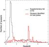 |
Fig. 9 Redshift distribution of quasars serendipitously identified quasars (black histogram) and identified on bad plates (red histogram). The number of objects for the black histogram is divided by 10 for clarity. |
In addition to this first supplementary list, we provide a list of quasars observed during the commissioning phase of the SDSS-III/BOSS spectrograph. Those objects were observed between MJD = 55 103 and MJD = 55 177 and were not re-observed later in the survey. This second supplementary list contains 291 quasars whose redshift distribution is also shown in Fig. 9 (red histogram). The spectra of those quasars are not part of the official DR12 (Alam et al. 2015) and are not available though the standard SDSS website. We provide an archival file that contains those 291 spectra.
The format of these two supplemental lists is detailed in Table 4.
Finally, these supplementary lists do not contain the spectra of all the AGNs available in the SDSS spectroscopic sample. In particular, there are objects targeted by the SDSS-III/BOSS galaxy survey that are spectroscopically classified as galaxies, but which show strong broad Mg ii in emission (Roig et al. 2014; Pattarakijwanich et al. 2014). These objects could not be selected as part of the superset described in Sect. 3 because of their classification by the SDSS pipeline.
7. Conclusion
We have presented the final quasar catalog of the SDSS-III/BOSS survey resulting from five years of observations. The catalog, which we call “DR12Q”, contains 297 301 quasars, 184 101 of which have z> 2.15. We provide robust identification from visual inspection and refined redshift measurements based on the result of a principal component analysis of the spectra. The present catalog contains about 80% more quasars than our previous release (Pâris et al. 2014). As part of DR12Q, we also provide a catalog of 29 579 BAL quasars and their properties. Spectroscopic line measurements are provided together with multi-wavelength matching with GALEX, 2MASS, UKIDSS, WISE, FIRST, RASS and XMM-Newton observations.
Observations for the fourth stage of the SDSS (SDSS-IV) started in July 2014. As part of the extended Baryonic Oscillation Spectroscopic Survey (eBOSS; Dawson et al. 2016), about half a million new quasars will be observed (Myers et al. 2015). In keeping with the growth rate of previous quasar surveys, SDSS-IV/eBOSS will expand the number of uniformly targeted quasars at redshifts 0.9 ≤ z ≤ 2.2 by more than an order of magnitude. The first spectroscopic release of SDSS-IV/eBOSS is expected to occur during the summer 2017.
The software used to reduce SDSS data is called idlspec2d. Its DR12 version is v5_7_0 for spectra taken prior to MJD = 56 755 and v5_7_3 after that date. Details can be found at http://www.sdss3.org/dr12/software and in Bolton et al. (2012).
Fan et al. (2001) reported a slightly different redshift for this quasar (z = 6.419) based on molecular ISM lines. The DR12Q redshift is solely based on the SDSS-III/BOSS spectrum.
Acknowledgments
I.P. was supported by PRIN INAF 2012 “The X-Shooter sample of 100 quasar spectra at z-3.5: Digging into cosmology and galaxy evolution with quasar absorption lines”. This work has been carried out thanks to the support of the A*MIDEX project (ANR-11-IDEX-0001-02) funded by the “Investissements d’Avenir” French Government program, managed by the French National Research Agency (ANR). The French Participation Group to SDSS-III was supported by the Agence Nationale de la Recherche under contracts ANR-08-BLAN-0222 and ANR-12-BS05-0015. A.D.M was partially supported by NASA ADAP award NNX12AE38G and by NSF awards 1211112 and 1515404. W.N.B. was supported by NSF grant AST-1516784. I.P. thanks S. Twain, D. Hoff, D. Dintei and Brian A. J. Richardson for their inspiring contribution to this work. Funding for SDSS-III has been provided by the Alfred P. Sloan Foundation, the Participating Institutions, the National Science Foundation, and the US Department of Energy Office of Science. The SDSS-III web site is http://www.sdss3.org/. SDSS-III is managed by the Astrophysical Research Consortium for the Participating Institutions of the SDSS-III Collaboration including the University of Arizona, the Brazilian Participation Group, Brookhaven National Laboratory, Carnegie Mellon University, University of Florida, the French Participation Group, the German Participation Group, Harvard University, the Instituto de Astrofisica de Canarias, the Michigan State/Notre Dame/JINA Participation Group, Johns Hopkins University, Lawrence Berkeley National Laboratory, Max Planck Institute for Astrophysics, Max Planck Institute for Extraterrestrial Physics, New Mexico State University, New York University, Ohio State University, Pennsylvania State University, University of Portsmouth, Princeton University, the Spanish Participation Group, University of Tokyo, University of Utah, Vanderbilt University, University of Virginia, University of Washington, and Yale University. AllWISE makes use of data from WISE, which is a joint project of the University of California, Los Angeles, and the Jet Propulsion Laboratory/California Institute of Technology, and NEOWISE, which is a project of the Jet Propulsion Laboratory/California Institute of Technology. WISE and NEOWISE are funded by the National Aeronautics and Space Administration. This research used resources of the National Energy Research Scientific Computing Center, a DOE Office of Science User Facility supported by the Office of Science of the US Department of Energy under Contract No. DE-AC02-05CH11231.
References
- Adelman-McCarthy, J. K., Agüeros, M. A., Allam, S. S., et al. 2008, ApJS, 175, 297 [NASA ADS] [CrossRef] [Google Scholar]
- Ahn, C. P., Alexandroff, R., Allen de Prieto, C., et al. 2012, ApJS, 203, 21 [NASA ADS] [CrossRef] [Google Scholar]
- Ahn, C. P., Alexandroff, R., Allen de Prieto, C., et al. 2014, ApJS, 211, 17 [NASA ADS] [CrossRef] [Google Scholar]
- Aihara, H., Allen de Prieto, C., An, D., et al. 2011, ApJS, 193, 29 [NASA ADS] [CrossRef] [Google Scholar]
- Alam, S., Albareti, F. D., Allen de Prieto, C., et al. 2015, ApJS, 219, 12 [NASA ADS] [CrossRef] [Google Scholar]
- Alam, S., Ata, M., Bailey, S., et al. 2016, ArXiv e-prints [arXiv:1607.03155] [Google Scholar]
- Albareti, F. D., Comparat, J., Gutiérrez, C. M., et al. 2015, MNRAS, 452, 4153 [NASA ADS] [CrossRef] [Google Scholar]
- Allen, J. T., Hewett, P. C., Maddox, N., Richards, G. T., & Belokurov, V. 2011, MNRAS, 410, 860 [NASA ADS] [CrossRef] [Google Scholar]
- Anderson, L., Aubourg, E., Bailey, S., et al. 2012, MNRAS, 427, 3435 [Google Scholar]
- Anderson, L., Aubourg, É., Bailey, S., et al. 2014, MNRAS, 441, 24 [NASA ADS] [CrossRef] [Google Scholar]
- Becker, R. H., White, R. L., & Helfand, D. J. 1995, ApJ, 450, 559 [NASA ADS] [CrossRef] [Google Scholar]
- Bolton, A. S., Schlegel, D. J., Aubourg, É., et al. 2012, AJ, 144, 144 [NASA ADS] [CrossRef] [Google Scholar]
- Bovy, J., Hennawi, J. F., Hogg, D. W., et al. 2011, ApJ, 729, 141 [NASA ADS] [CrossRef] [Google Scholar]
- Bovy, J., Myers, A. D., Hennawi, J. F., et al. 2012, ApJ, 749, 41 [NASA ADS] [CrossRef] [Google Scholar]
- Boyle, B. J., Shanks, T., & Peterson, B. A. 1988, MNRAS, 235, 935 [NASA ADS] [Google Scholar]
- Busca, N. G., Delubac, T., Rich, J., et al. 2013, A&A, 552, A96 [NASA ADS] [CrossRef] [EDP Sciences] [Google Scholar]
- Croom, S. M., Smith, R. J., Boyle, B. J., et al. 2004, MNRAS, 349, 1397 [NASA ADS] [CrossRef] [Google Scholar]
- Cutri, R. M., Skrutskie, M. F., van Dyk, S., et al. 2003, VizieR Online Data Catalog: II/246 [Google Scholar]
- Dawson, K. S., Schlegel, D. J., Ahn, C. P., et al. 2013, AJ, 145, 10 [Google Scholar]
- Dawson, K. S., Kneib, J.-P., Percival, W. J., et al. 2016, AJ, 151, 44 [NASA ADS] [CrossRef] [Google Scholar]
- Delubac, T., Bautista, J. E., Busca, N. G., et al. 2015, A&A, 574, A59 [NASA ADS] [CrossRef] [EDP Sciences] [Google Scholar]
- Diamond-Stanic, A. M., Fan, X., Brandt, W. N., et al. 2009, ApJ, 699, 782 [NASA ADS] [CrossRef] [Google Scholar]
- Eftekharzadeh, S., Myers, A. D., White, M., et al. 2015, MNRAS, 453, 2779 [NASA ADS] [CrossRef] [Google Scholar]
- Eisenstein, D. J., Weinberg, D. H., Agol, E., et al. 2011, AJ, 142, 72 [Google Scholar]
- Elvis, M., Lockman, F. J., & Fassnacht, C. 1994, ApJS, 95, 413 [NASA ADS] [CrossRef] [EDP Sciences] [Google Scholar]
- Fan, X., Narayanan, V. K., Lupton, R. H., et al. 2001, AJ, 122, 2833 [NASA ADS] [CrossRef] [Google Scholar]
- Font-Ribera, A., Kirkby, D., Busca, N., et al. 2014, J. Cosmol. Astropart. Phys., 5, 27 [Google Scholar]
- Fukugita, M., Ichikawa, T., Gunn, J. E., et al. 1996, AJ, 111, 1748 [NASA ADS] [CrossRef] [Google Scholar]
- Gibson, R. R., Jiang, L., Brandt, W. N., et al. 2009, ApJ, 692, 758 [NASA ADS] [CrossRef] [Google Scholar]
- Gunn, J. E., Carr, M., Rockosi, C., et al. 1998, AJ, 116, 3040 [NASA ADS] [CrossRef] [Google Scholar]
- Gunn, J. E., Siegmund, W. A., Mannery, E. J., et al. 2006, AJ, 131, 2332 [NASA ADS] [CrossRef] [Google Scholar]
- Hall, P. B., Anderson, S. F., Strauss, M. A., et al. 2002, ApJS, 141, 267 [NASA ADS] [CrossRef] [Google Scholar]
- Hewett, P. C., & Wild, V. 2010, MNRAS, 405, 2302 (HW10) [NASA ADS] [Google Scholar]
- Hewett, P. C., Foltz, C. B., & Chaffee, F. H. 1995, AJ, 109, 1498 [NASA ADS] [CrossRef] [Google Scholar]
- Hogg, D. W., Finkbeiner, D. P., Schlegel, D. J., & Gunn, J. E. 2001, AJ, 122, 2129 [NASA ADS] [CrossRef] [Google Scholar]
- Ivezić, Ž., Lupton, R. H., Schlegel, D., et al. 2004, Astron. Nachr., 325, 583 [NASA ADS] [CrossRef] [Google Scholar]
- Kaiser, N., Aussel, H., Burke, B. E., et al. 2002, in Survey and Other Telescope Technologies and Discoveries, eds. J. A. Tyson & S. Wolff, SPIE Conf. Ser., 4836, 154 [Google Scholar]
- Kaiser, N., Burgett, W., Chambers, K., et al. 2010, in SPIE Conf. Ser. 7733, 77330E [Google Scholar]
- Kirkpatrick, J. A., Schlegel, D. J., Ross, N. P., et al. 2011, ApJ, 743, 125 [NASA ADS] [CrossRef] [Google Scholar]
- Krawczyk, C. M., Richards, G. T., Mehta, S. S., et al. 2013, ApJS, 206, 4 [NASA ADS] [CrossRef] [Google Scholar]
- LaMassa, S. M., Cales, S., Moran, E. C., et al. 2015, ApJ, 800, 144 [NASA ADS] [CrossRef] [Google Scholar]
- Law, N. M., Kulkarni, S. R., Dekany, R. G., et al. 2009, PASP, 121, 1395 [NASA ADS] [CrossRef] [Google Scholar]
- Lawrence, A., Warren, S. J., Almaini, O., et al. 2007, MNRAS, 379, 1599 [NASA ADS] [CrossRef] [MathSciNet] [Google Scholar]
- Lupton, R., Gunn, J. E., Ivezić, Z., et al. 2001, in Astronomical Data Analysis Software and Systems X, eds. F. R. Harnden Jr., F. A. Primini, & H. E. Payne, ASP Conf. Ser., 238, 269 [Google Scholar]
- Lupton, R. H., Gunn, J. E., & Szalay, A. S. 1999, AJ, 118, 1406 [NASA ADS] [CrossRef] [Google Scholar]
- Mainzer, A., Bauer, J., Grav, T., et al. 2011, ApJ, 731, 53 [NASA ADS] [CrossRef] [Google Scholar]
- Martin, D. C., Fanson, J., Schiminovich, D., et al. 2005, ApJ, 619, L1 [Google Scholar]
- McDonald, P., & Eisenstein, D. J. 2007, Phys. Rev. D, 76, 063009 [NASA ADS] [CrossRef] [Google Scholar]
- Merloni, A., Dwelly, T., Salvato, M., et al. 2015, MNRAS, 452, 69 [NASA ADS] [CrossRef] [Google Scholar]
- Morganson, E., Green, P. J., Anderson, S. F., et al. 2015, ApJ, 806, 244 [NASA ADS] [CrossRef] [Google Scholar]
- Myers, A. D., Palanque-Delabrouille, N., Prakash, A., et al. 2015, ApJS, 221, 27 [NASA ADS] [CrossRef] [Google Scholar]
- Ofek, E. O., Laher, R., Surace, J., et al. 2012, PASP, 124, 854 [NASA ADS] [CrossRef] [Google Scholar]
- Oke, J. B., & Gunn, J. E. 1983, ApJ, 266, 713 [NASA ADS] [CrossRef] [Google Scholar]
- Osmer, P. S., & Smith, M. G. 1980, ApJS, 42, 333 [NASA ADS] [CrossRef] [Google Scholar]
- Padmanabhan, N., Schlegel, D. J., Finkbeiner, D. P., et al. 2008, ApJ, 674, 1217 [NASA ADS] [CrossRef] [MathSciNet] [Google Scholar]
- Palanque-Delabrouille, N., Yèche, C., Myers, A. D., et al. 2011, A&A, 530, A122 [NASA ADS] [CrossRef] [EDP Sciences] [Google Scholar]
- Palanque-Delabrouille, N., Magneville, C., Yèche, C., et al. 2013, A&A, 551, A29 [NASA ADS] [CrossRef] [EDP Sciences] [Google Scholar]
- Pâris, I., Petitjean, P., Rollinde, E., et al. 2011, A&A, 530, A50 [NASA ADS] [CrossRef] [EDP Sciences] [Google Scholar]
- Pâris, I., Petitjean, P., Aubourg, É., et al. 2012, A&A, 548, A66 [NASA ADS] [CrossRef] [EDP Sciences] [Google Scholar]
- Pâris, I., Petitjean, P., Aubourg, É., et al. 2014, A&A, 563, A54 [NASA ADS] [CrossRef] [EDP Sciences] [Google Scholar]
- Pattarakijwanich, P., Strauss, M. A., Ho, S., & Ross, N. P. 2014, ArXiv e-prints [arXiv:1410.7394] [Google Scholar]
- Peters, C. M., Richards, G. T., Myers, A. D., et al. 2015, ApJ, 811, 95 [NASA ADS] [CrossRef] [Google Scholar]
- Pier, J. R., Munn, J. A., Hindsley, R. B., et al. 2003, AJ, 125, 1559 [NASA ADS] [CrossRef] [Google Scholar]
- Rau, A., Kulkarni, S. R., Law, N. M., et al. 2009, PASP, 121, 1334 [NASA ADS] [CrossRef] [Google Scholar]
- Reid, B., Ho, S., Padmanabhan, N., et al. 2016, MNRAS, 455, 1553 [NASA ADS] [CrossRef] [Google Scholar]
- Richards, G. T., Nichol, R. C., Gray, A. G., et al. 2004, ApJS, 155, 257 [NASA ADS] [CrossRef] [Google Scholar]
- Richards, G. T., Strauss, M. A., Fan, X., et al. 2006, AJ, 131, 2766 [NASA ADS] [CrossRef] [Google Scholar]
- Richards, G. T., Myers, A. D., Gray, A. G., et al. 2009, ApJS, 180, 67 [NASA ADS] [CrossRef] [Google Scholar]
- Roig, B., Blanton, M. R., & Ross, N. P. 2014, ApJ, 781, 72 [NASA ADS] [CrossRef] [Google Scholar]
- Ross, N. P., Myers, A. D., Sheldon, E. S., et al. 2012, ApJS, 199, 3 [NASA ADS] [CrossRef] [Google Scholar]
- Ross, N. P., McGreer, I. D., White, M., et al. 2013, ApJ, 773, 14 [NASA ADS] [CrossRef] [Google Scholar]
- Schlafly, E. F., & Finkbeiner, D. P. 2011, ApJ, 737, 103 [NASA ADS] [CrossRef] [Google Scholar]
- Schlegel, D. J., Finkbeiner, D. P., & Davis, M. 1998, ApJ, 500, 525 [NASA ADS] [CrossRef] [Google Scholar]
- Schmidt, K. B., Marshall, P. J., Rix, H.-W., et al. 2010, ApJ, 714, 1194 [NASA ADS] [CrossRef] [Google Scholar]
- Schmidt, M. 1963, Nature, 197, 1040 [NASA ADS] [CrossRef] [Google Scholar]
- Schmidt, M., & Green, R. F. 1983, ApJ, 269, 352 [NASA ADS] [CrossRef] [Google Scholar]
- Schneider, D. P., Hall, P. B., Richards, G. T., et al. 2007, AJ, 134, 102 [NASA ADS] [CrossRef] [Google Scholar]
- Schneider, D. P., Richards, G. T., Hall, P. B., et al. 2010, AJ, 139, 2360 [NASA ADS] [CrossRef] [Google Scholar]
- Shen, Y., Brandt, W. N., Denney, K. D., et al. 2016, ApJ, 831, 7 [NASA ADS] [CrossRef] [Google Scholar]
- Skrutskie, M. F., Cutri, R. M., Stiening, R., et al. 2006, AJ, 131, 1163 [NASA ADS] [CrossRef] [Google Scholar]
- Slosar, A., Iršič, V., Kirkby, D., et al. 2013, J. Cosmol. Astropart. Phys., 4, 26 [Google Scholar]
- Smee, S. A., Gunn, J. E., Uomoto, A., et al. 2013, AJ, 146, 32 [Google Scholar]
- Smith, J. A., Tucker, D. L., Kent, S., et al. 2002, AJ, 123, 2121 [Google Scholar]
- Spergel, D. N., Verde, L., Peiris, H. V., et al. 2003, ApJS, 148, 175 [NASA ADS] [CrossRef] [Google Scholar]
- Stark, A. A., Gammie, C. F., Wilson, R. W., et al. 1992, ApJS, 79, 77 [NASA ADS] [CrossRef] [Google Scholar]
- Storrie-Lombardi, L. J., McMahon, R. G., Irwin, M. J., & Hazard, C. 1996, ApJ, 468, 121 [NASA ADS] [CrossRef] [Google Scholar]
- Stoughton, C., Lupton, R. H., Bernardi, M., et al. 2002, AJ, 123, 485 [NASA ADS] [CrossRef] [Google Scholar]
- Trump, J. R., Hall, P. B., Reichard, T. A., et al. 2006, ApJS, 165, 1 [NASA ADS] [CrossRef] [Google Scholar]
- Tucker, D. L., Kent, S., Richmond, M. W., et al. 2006, Astron. Nachr., 327, 821 [NASA ADS] [CrossRef] [Google Scholar]
- Voges, W., Aschenbach, B., Boller, T., et al. 1999, A&A, 349, 389 [NASA ADS] [Google Scholar]
- Voges, W., Aschenbach, B., Boller, T., et al. 2000, IAU Circ., 7432, 3 [NASA ADS] [Google Scholar]
- Watson, M. G., Schröder, A. C., Fyfe, D., et al. 2009, A&A, 493, 339 [NASA ADS] [CrossRef] [EDP Sciences] [Google Scholar]
- Wells, D. C., Greisen, E. W., & Harten, R. H. 1981, A&AS, 44, 363 [NASA ADS] [Google Scholar]
- Weymann, R. J., Morris, S. L., Foltz, C. B., & Hewett, P. C. 1991, ApJ, 373, 23 [NASA ADS] [CrossRef] [Google Scholar]
- White, M., Myers, A. D., Ross, N. P., et al. 2012, MNRAS, 424, 933 [NASA ADS] [CrossRef] [Google Scholar]
- Wright, E. L., Eisenhardt, P. R. M., Mainzer, A. K., et al. 2010, AJ, 140, 1868 [Google Scholar]
- Yèche, C., Petitjean, P., Rich, J., et al. 2010, A&A, 523, A14 [NASA ADS] [CrossRef] [EDP Sciences] [Google Scholar]
- York, D. G., Adelman, J., Anderson, Jr., J. E., et al. 2000, AJ, 120, 1579 [CrossRef] [Google Scholar]
Appendix A: List of target selection flags
Detailed result of visual inspection of DR12 quasar targets for each target selection bit.
Appendix B: Description of the superset of DR12Q
Description of the file that contains the superset from which we derive the DR12Q catalog.
Appendix C: Additional table
DR12Q catalog format.
All Tables
Number of objects identified as such by the pipeline with any ZWARNING value (second column) and with ZWARNING = 0 (third column), and after the visual inspection (fourth column).
Format of the binary FITS file that contains “trough-by-trough” information for BAL quasars.
Detailed result of visual inspection of DR12 quasar targets for each target selection bit.
Description of the file that contains the superset from which we derive the DR12Q catalog.
All Figures
|
Fig. 1 Distribution on the sky of the SDSS-DR12/BOSS spectroscopy in J2000 equatorial coordinates (expressed in decimal degrees). |
| In the text | |
|
Fig. 2 Cumulative number of quasars as a function of observation date during the whole SDSS-III/BOSS survey. A total of 297 301 quasars was spectroscopically confirmed. The “flat portions” in this figure correspond to summer shutdowns. |
| In the text | |
|
Fig. 3 Examples of spectra identified as QSO_? (top left), QSO_Z? (middle left), QSO_BAL_Z? (bottom left), Star_? (top right), ? (middle right), and Bad (bottom right). The fluxes are shown in black and associated errors in green. All the spectra are smoothed over 10 pixels. |
| In the text | |
|
Fig. 4 Left panel: redshift distribution of the SDSS-DR12 (thick black histogram), SDSS-DR10 (orange histogram) and SDSS-DR7 (blue histogram) quasars over the redshift range 0–6. Right panel: redshift distribution of the SDSS-DR12 quasars for the CORE sample (dark blue histogram), BONUS sample (light blue histogram), ancillary programs (red histogram) and SEQUELS (orange histogram). The bin size of all the histograms is Δz = 0.05. The two peaks at z ~ 0.8 and z ~ 1.6 seen in the redshift distribution of the SDSS-DR10 and SDSS-DR12 quasar samples (left panel) and in the distribution of the CORE and BONUS samples (right panel) are due to known degeneracies in the quasar target selection (see Ross et al. 2012,for details). |
| In the text | |
|
Fig. 5 Left panel: distribution of r PSF magnitude (corrected for Galactic extinction) for the BOSS main sample (selected by the algorithms described in Ross et al. 2012,thick black histogram), ancillary programs (red histogram) and SEQUELS (orange histogram). The bin size is Δr = 0.02. Right panel: absolute magnitude-redshift plane for SDSS-DR12 CORE+BONUS quasars (black contours), quasars observed as part of SDSS-DR12 ancillary programs (red points), SEQUELS quasars (orange points) and SDSS-DR7 quasars (blue contours). The absolute magnitudes assume H0 = 70 km s-1 Mpc-1 and the K-correction is given by Richards et al. (2006), who define K(z = 2) = 0. Contours are drawn at constant point density. |
| In the text | |
|
Fig. 6 Spectrum of the highest redshift (z = 6.440) quasar observed by BOSS is displayed in the top left panel. This quasar was discovered by Fan et al. (2001). Typical spectra of SEQUELS quasars are presented at five different redshifts: z ~ 1.2 (top right panel) and z ~ 1.6 (middle left panel). Typical BOSS quasars are shown at three different redshifts: z ~ 2.2 (middle right panel), z ~ 2.7 (bottom left panel) and z ~ 3.5 (bottom right panel). All the spectra are smoothed over 5 pixels. |
| In the text | |
|
Fig. 7 Distribution of velocity differences between the visual inspection redshift (Z_VI, black histogram), Mg ii-based redshift (Z_MGII, red histogram), SDSS pipeline redshift (Bolton et al. 2012,blue histogram), C iv-based redshift (Z_CIV, green histogram), C iii]-based redshift (Z_CIII, cyan histogram) and the PCA redshift (Z_PCA). The bin size of all the histograms is Δv = 50 km s-1. |
| In the text | |
|
Fig. 8 Left panel: distribution of AI for the SDSS-DR3 (magenta histogram; Trump et al. 2006) and the SDSS-DR12 (black histogram) quasars. Both distributions are normalized to have a surface area equal to 1 for log AI > 2.5. Right panel: distribution of BI from the DR12Q catalog (black histogram), from the SDSS-DR6 (red histogram; Allen et al. 2011) and from the SDSS-DR5 (blue histogram; Gibson et al. 2009). All the distributions are normalized to have their sum equal to 1. |
| In the text | |
|
Fig. 9 Redshift distribution of quasars serendipitously identified quasars (black histogram) and identified on bad plates (red histogram). The number of objects for the black histogram is divided by 10 for clarity. |
| In the text | |
Current usage metrics show cumulative count of Article Views (full-text article views including HTML views, PDF and ePub downloads, according to the available data) and Abstracts Views on Vision4Press platform.
Data correspond to usage on the plateform after 2015. The current usage metrics is available 48-96 hours after online publication and is updated daily on week days.
Initial download of the metrics may take a while.