| Issue |
A&A
Volume 596, December 2016
|
|
|---|---|---|
| Article Number | A45 | |
| Number of page(s) | 18 | |
| Section | Extragalactic astronomy | |
| DOI | https://doi.org/10.1051/0004-6361/201528034 | |
| Published online | 28 November 2016 | |
The F-GAMMA programme: multi-frequency study of active galactic nuclei in the Fermi era
Programme description and the first 2.5 years of monitoring⋆
1 Max-Planck-Institut für Radioastronomie, Auf dem Hügel 69, 53121 Bonn, Germany
e-mail: lfuhrmann@mpifr-bonn.mpg.de
2 IAPS-INAF, via Fosso del Cavaliere 100, 00133 Roma, Italy
3 Department of Physics/ Institute for Plasma Physics, University of Crete, and FORTH-IESL, 71003 Heraklion, Greece
4 California Institute of Technology, Pasadena, CA 91125, USA
5 Instituto de Radioastronomía Milimétrica, Avenida Divina Pastora 7, Local 20, 18012 Granada, Spain
6 KTH Royal Institute of Technology, Departement of Physics, AlbaNova, 10691 Stockholm, Sweden
7 Oskar Klein Centre, Department of Astronomy, AlbaNova, 10691 Stockholm, Sweden
8 Department of Physics, Purdue University, 525 Northwestern Ave, West Lafayette, IN 47907, USA
9 University of Science and Technology, 133 Gwahangno, Yuseong-gu, Daejeon, 305-333, Republic of Korea
10 Korea Astronomy and Space Science Institute, 776 Daedeok-Daero, Yuseong-gu, Daejeon, 305-348, Republic of Korea
Received: 23 December 2015
Accepted: 4 August 2016
Context. To fully exploit the scientific potential of the Fermi mission for the physics of active galactic nuclei (AGN), we initiated the F-GAMMA programme. Between 2007 and 2015 the F-GAMMA was the prime provider of complementary multi-frequency monitoring in the radio regime.
Aims. We quantify the radio variability of γ-ray blazars. We investigate its dependence on source class and examine whether the radio variability is related to the γ-ray loudness. Finally, we assess the validity of a putative correlation between the two bands.
Methods. The F-GAMMA performed monthly monitoring of a sample of about 60 sources at up to twelve radio frequencies between 2.64 and 228.39 GHz. We perform a time series analysis on the first 2.5-yr data set to obtain variability parameters. A maximum likelihood analysis is used to assess the significance of a correlation between radio and γ-ray fluxes.
Results. We present light curves and spectra (coherent within ten days) obtained with the Effelsberg 100 m and IRAM 30 m telescopes. All sources are variable across all frequency bands with amplitudes increasing with frequency up to rest frame frequencies of around 60–80 GHz as expected by shock-in-jet models. Compared to flat-spectrum radio quasars (FSRQs), BL Lacertae objects (BL Lacs) show systematically lower variability amplitudes, brightness temperatures, and Doppler factors at lower frequencies, while the difference vanishes towards higher ones. The time scales appear similar for the two classes. The distribution of spectral indices appears flatter or more inverted at higher frequencies for BL Lacs. Evolving synchrotron self-absorbed components can naturally account for the observed spectral variability. We find that the Fermi-detected sources show larger variability amplitudes, brightness temperatures, and Doppler factors than non-detected ones. Flux densities at 86.2 and 142.3 GHz correlate with 1 GeV fluxes at a significance level better than 3σ, implying that γ rays are produced very close to the mm-band emission region.
Key words: galaxies: active / BL Lacertae objects: general / quasars: general / galaxies: jets / gamma rays: galaxies / radiation mechanisms: non-thermal
Tables of the measured fluxes are only available at the CDS via anonymous ftp to cdsarc.u-strasbg.fr (130.79.128.5) or via http://cdsarc.u-strasbg.fr/viz-bin/qcat?J/A+A/596/A45
© ESO, 2016
1. Introduction
Powerful jets, sometimes extending outwards to several Mpc from a bright nucleus, are the most striking feature of radio-loud active galactic nuclei (AGN). It is theorised that the power sustaining these systems is extracted through the infall of galactic material onto a supermassive black hole via an accretion flow. Material is then channeled to jets which transport angular momentum and energy away from the active nucleus in the intergalactic space (Blandford & Rees 1974; Hargrave & Ryle 1974). Unification theories attribute the phenomenological variety of AGN types to the combination of their intrinsic energy output and orientation of their jets relative to our line of sight (Readhead et al. 1978; Blandford & Königl 1979; Readhead 1980; Urry & Padovani 1995).
Blazars, viewed at angles not larger than 10° to 20°, form the sub-class of radio-loud AGN showing the most extreme phenomenology. This typically involves strong broadband variability, a high degree of optical polarisation, apparent superluminal motions (e.g. Dent 1966; Cohen et al. 1971; Shaffer et al. 1972), and a unique broadband double-humped spectral energy distribution (SED; Urry 1999). Moreover, blazars have long been established as a group of bright and highly variable γ-ray sources (e.g. Hartman et al. 1992). While different processes may occur in different objects, the high-energy blazar emission is believed to be produced by the inverse Compton (IC) mechanism acting on seed photons inside the jet (synchrotron self-Compton, SSC) or external Compton (EC) acting on photons from the broad-line region (BLR) or the accretion disk (leptonic models, e.g. Dermer et al. 1992; Böttcher 2007). Alternatively, proton induced cascades and their products have been invoked to account for this emission in the case of hadronic jets (e.g. Mannheim 1993).
Despite all efforts, several key questions still remain unanswered, for example: (i) what are the dominant, broadband emission processes; (ii) which mechanisms drive the violent, broadband variability of blazars; and (iii) what is the typical duty cycle of their activity? A number of competing models attempt to explain their observed properties in terms of e.g. relativistic shock-in-jet models (e.g. Marscher & Gear 1985; Valtaoja et al. 1992; Türler 2011) or colliding relativistic plasma shells (e.g. Spada et al. 2001; Guetta et al. 2004). Quasi-periodicities seen in the long-term variability curves on time scales of months to years may indicate systematic changes in the beam orientation (lighthouse effect: Camenzind & Krockenberger 1992), possibly related to binary black hole systems, MHD instabilities in the accretion disks, and/or helical/precessing jets (e.g. Begelman et al. 1980; Carrara et al. 1993; Villata & Raiteri 1999). Finally, the location of γ-ray emission is still intensely debated (cf. Blandford & Levinson 1995; Valtaoja & Teräsranta 1995; Jorstad et al. 2001; Marscher 2014).
Analysis and theoretical modelling of quasi-simultaneous spectral variability over spectral ranges that are as broad as possible (radio to GeV/TeV energies) allows the detailed study of different emission mechanisms and comparison with different competing theories. Hence, variability studies furnish important clues about the size, structure, physics, and dynamics of the emitting region making AGN/blazar monitoring programmes extremely important in providing the necessary constraints for understanding the origin of energy production.
Examples of past and ongoing long-term radio monitoring programmes with variability studies are the University of Michigan Radio Observatory (UMRAO) Program (4.8–14.5 GHz; e.g. Aller 1970; Aller et al. 1985), the monitoring at the Medicina/Noto 32 m telescopes (5, 8, 22 GHz; Bach et al. 2007), and the RATAN-600 monitoring (1–22 GHz; Kovalev et al. 2002), all at lower radio frequencies. At intermediate frequencies, the Metsähovi Radio Observatory programme (22 and 37 GHz; e.g. Salonen et al. 1987; Valtaoja et al. 1988) is one example, while at high frequencies the IRAM 30 m monitoring programme (90, 150, 230 GHz; e.g. Steppe et al. 1988, 1992; Ungerechts et al. 1998) is another. Nevertheless, the lack of continuous observations at all wave bands and the historical lack of sufficient γ-ray data prevented past efforts from studying the broadband jet emission in detail.
The launch of the Fermi Gamma-ray Space Telescope (Fermi) in June 2008, with its high cadence “all-sky monitor” capabilities, has introduced a new era in the field of AGN astrophysics providing a remarkable opportunity for attacking the crucial questions outlined above. The Large Area Telescope (LAT; Atwood et al. 2009) on board Fermi constitutes a large leap compared to its predecessor, the Energetic Gamma-ray Experiment Telescope (EGRET). Since 2008, Fermi has gathered spectacular γ-ray spectra and light curves resolved at a variety of time scales for about 1500 AGN (e.g. Abdo et al. 2010d; Ackermann et al. 2011b, 2015).
The Fermi-GST AGN Multi-frequency Monitoring Alliance (F-GAMMA) represents an effort, highly coordinated with Fermi and other observatories, for the monitoring of selected AGN. Here, we present F-GAMMA and report on the results obtained for the initial sample, during the first 2.5 yr of observations (January 2007 to June 2009). The paper is structured as follows. In Sect. 2 we introduce the programme, discuss the sample selection, describe the participating observatories, and outline the data reduction. Sections 3–5 present the variability analysis, the connection between radio variability and γ-ray loudness, and the radio and γ-ray flux-flux correlation, respectively. We summarise our results and conclude in Sect. 6.
2. The F-GAMMA programme
The F-GAMMA programme (Fuhrmann et al. 2007; Angelakis et al. 2010; Fuhrmann et al. 2014; Angelakis et al. 2015) aimed at providing a systematic monthly monitoring of the radio emission of about 60 γ-ray blazars over the frequency range from 2.64 to 345 GHz. The motivation was the acquisition of uniformly sampled light curves meant to
-
complement the Fermi light curves and other, ideallysimultaneous, data sets for the construction of coherent SEDs(e.g. Giommiet al. 2012);
-
be used for studying the evolutionary tracks of spectral components as well as variability studies (e.g. shock models Valtaoja et al. 1992, Fromm et al. 2015);
-
be used for cross-band correlations and time series analyses (e.g. Fuhrmann et al. 2014; Karamanavis et al. 2016a);
-
correlations with source structural evolution studies (Karamanavis et al. 2016b).
Below we explain the sample selection and then the observations and the data reduction for each facility separately.
2.1. Sample selection
Initial F-GAMMA sample monitored at EB and PV between January 2007 and June 2009.
The selection of the F-GAMMA source sample was determined by our goal to understand the physical processes in γ-ray-loud blazars; in particular their broadband variability and spectral evolution during periods of energetically violent outbursts. By definition, the programme was designed to take advantage of the continuous Fermi monitoring of the entire sky. Since the F-GAMMA observations started more than a year before the Fermi launch, the monitored sample was subjected to a major update (in mid-2009) once the first Fermi lists were released to include only sources monitored by the satellite.
Initially, the F-GAMMA sample included 62 sources selected to satisfy several criteria. The most important of which were the following:
-
1.
The sources should be previously detected in γ rays by EGRET and be included in the “high-priority AGN/blazar list” released by the Fermi/LAT AGN working group, which would tag them as potential Fermi γ-ray candidates.
-
2.
They should display flat radio spectra, an identifying characteristic of blazar behaviour.
-
3.
They should comply with certain observational constraints, i.e. they should be at relatively high declination (δ ≥ −30°) and give high average brightness to allow uninterruptedly reliable and high-quality data flow.
-
4.
They should show frequent activity – in as many energy bands as possible – to allow cross-band and variability studies.
In Table 1, we list the sources in the initial sample that were observed with the Effelsberg and IRAM telescopes between January 2007 and June 2009, which is the period covered by the present work. The Effelsberg and IRAM observations were done monthly and in a highly synchronised manner. A sub-set of 24 of these sources and an additional sample of about 20 southern γ-ray AGN were observed also with the APEX telescope (see Larsson et al. 2012).
An important consideration during the sample selection was the overlap with other campaigns and particularly VLBI monitoring programme. Most of the 62 sources in our sample (95%) are included in the IRAM polarisation monitoring (POLAMI; e.g. Agudo et al. 2014). A major fraction (89%) were observed by MOJAVE (Lister et al. 2009), and almost half (47%) are in the Boston 43 GHz Program (Jorstad et al. 2005). One-third of our sources (27%) are in the GMVA monitoring and one source (namely PKS 2155-304) is part of the southern TANAMI VLBI Program (Ojha et al. 2010). The Third EGRET Catalog (Hartman et al. 1999) includes 40% of the initial sample sources while the majority of sources (69%) are in CGRaBS. WMAP Point Source Catalog (Bennett et al. 2003) includes 61% of our sample and 74% are in the Planck Early Release Compact Source Catalogue (ERCSC, Planck Collaboration et al. 2011). The last column of Table 1 summarises the overlap with all these programmes.
On the basis of the classical AGN classification scheme – flat-spectrum radio quasars (FSRQs), BL Lacertae objects (BL Lacs), and radio galaxies (e.g. Urry & Padovani 1995) – the initial F-GAMMA sample consists of 32 FSRQs (52%), 23 BL Lacs (37%), 3 radio galaxies (5%), and 3 unclassified blazars (5%).
In June 2009, soon after the release of the first Fermi source lists (LBAS and 1LAC; Abdo et al. 2009b, 2010c), the F-GAMMA sample was partially revised to include exclusively Fermi monitored sources. The revised list will be presented in Nestoras et al. (2016) and Angelakis et al. (in prep.).
2.2. Observations and data reduction
The main facilities employed for the F-GAMMA programme were the Effelsberg 100 m (hereafter EB), IRAM 30 m (PV), and APEX 12 m telescopes. The observations were highly coordinated between the EB and PV. In addition, as has already been discussed, several other facilties and teams have occasionally participated in campaigns in collaboration with the F-GAMMA programme or have provided complementary studies. Here we summarise the involved facilites, the associated data acquisition, and reduction.
Top: participating facilities of the F-GAMMA programme. Bottom: telescopes of the main collaborations and complementary projects.
2.2.1. The Effelsberg 100 m telescope
The most important facility for the F-GAMMA programme has been the Effelsberg 100 m telescope owing to the broad frequency coverage, the large number of available receivers in that range, and the high measurement precision.
The observations started in January 2007 and stopped in January 2015. Here, however, we focus only on the first 2.5 yr over which the initial F-GAMMA sample was monitored. The programme was scheduled monthly in 30- to 40-h sessions. The observations were conducted with the eight secondary focus receivers listed in Table 2 covering the range from 2.64 to 43 GHz in total power and polarisation (whenever available). Their detailed characteristics are listed in Table 4 of Angelakis et al. (2015).
The measurements were done with “cross-scans” i.e. by measuring the telescope response as it progressively slews over the source position in azimuth and elevation direction. This technique allows the correction of small pointing offsets, the detection of possible spatial extension of a source, or cases of confusion from field sources. The systems at 4.85, 10.45, and 32 GHz are equipped with multiple feeds which were used for subtracting tropospheric effects (“beam switch”). The time needed to obtain a whole spectrum was of the order of 35–40 min, guaranteeing measurements free of source variability.
The data reduction and the post-measurement data processing is described in Sect. 3 of Angelakis et al. (2015). For the absolute calibration we used the reference sources 3C 48, 3C 161, 3C 286, 3C 295, and NGC 7027 (Baars et al. 1977; Ott et al. 1994; Zijlstra et al. 2008). The assumed flux density values for each frequency are listed in Table 3 of Angelakis et al. (2015). The overall measurement uncertainties are of the order of ≤ 1% and ≤ 5% at lower and higher frequencies, respectively.
2.2.2. The IRAM 30 m telescope
The IRAM 30 m telescope at Pico Veleta covered the important short-mm bands. The observations started in June 2007 and stopped in May 2014 using the “B” and “C” SIS heterodyne receivers at 86.2 (500 MHz bandwidth), 142.3, and 228.9 GHz both with 1 GHz bandwidth (Table 2). The receivers were operated in a single linear polarisation mode, but simultaneously at the three observing frequencies.
To minimise the influence of blazar variability in the combined spectra, the EB and PV observations were synchronised typically within a few days up to about one week. The F-GAMMA observations were combined with the general flux monitoring conducted by IRAM (e.g. Ungerechts et al. 1998). The data presented here come from both programmes.
Observations were performed with calibrated cross-scans in the azimuth and elevation directions. For each target the cross-scans were preceded by a calibration scan to obtain instantaneous opacity information and convert the counts to the antenna temperature scale  corrected for atmospheric attenuation as described by Mauersberger et al. (1989). After a necessary quality flagging, the sub-scans in each scanning direction were averaged and fitted with Gaussian curves. Each fitted amplitude was then corrected for pointing offsets and elevation-dependent losses. The absolute calibration was done with reference to frequently observed primary (Mars, Uranus) and secondary calibrators (W3(OH), K3-50A, NGC 7027). The overall measurement uncertainties are 5–10%.
2.3. Other facilities
In order to accommodate the needs for broader frequency coverage, dense monitoring of large unbiased samples and synchronous monitoring of structural evolution a number of collaborating facilities were coordinated with the F-GAMMA programme. For completeness they are briefly described below.
The APEX sub-mm telescope: in 2008, we started using the Large Apex Bolometer Camera (LABOCA; Siringo et al. 2008) of the Atacama Pathfinder EXperiment (APEX) 12 m telescope to obtain light curves at 345 GHz for a sub-set of 25 F-GAMMA sources and 14 southern hemisphere γ-ray AGN. In the current paper we do not present APEX data. The first results, however, are discussed in Larsson et al. (2012).
The OVRO 40-m programme: in mid-2007 a programme complementary to F-GAMMA was commenced at the OVRO 40 m telescope. It is dedicated to the dense monitoring of a large sample of blazars at 15 GHz. The initial sample included 1158 CGRaBS sources (Healey et al. 2008) with declination ≥−20°. The sample was later enriched with Fermi-detected sources data to reach a size of around 1800. The cadence is around a few days. The details of the OVRO programme are discussed by Richards et al. (2011, 2014).
Korean VLBI Network programme: the AGN group of the Korean VLBI Network (KVN) has been using the KVN antennas since 2010 for the monthly monitoring of γ-ray blazars simultaneously at 22 and 42 GHz (Lee et al. 2011). Details of the observing method can be found in Park et al. (2013).
Optical monitoring: in collaboration with the California Institute of Technology (Caltech), the University of Crete, the Inter-University Centre for Astronomy and Astrophysics (IUCAA), and the Torun Center for Astronomy at the Nicolaus Copernicus University, we initiated, funded, and constructed the RoboPol optical polarimeter (King et al. 2014) mounted on the 1.3 m Skinakas optical telescope (Greece). Since 2013 RoboPol has been monitoring the optical linear polarisation of a sample of 60 blazars including 47 F-GAMMA sources. The first polarisation results of RoboPol are presented in Pavlidou et al. (2014), Blinov et al. (2015, 2016) and Angelakis et al. (2016).
3. Variability analysis
Here we study the initial F-GAMMA sample. We focus on the first 2.5 yr of EB observations (31 sessions from January 2007 to June 2009) and the first 2 yr of monitoring with PV (21 sessions from June 2007 to June 2009).
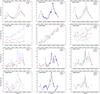 |
Fig. 1 Combined EB and PV light curves for selected, particularly active Fermi sources of the F-GAMMA sample. Data obtained within the OVRO 40 m programme at 15 GHz are also shown. Left: low frequencies (2.64, 4.85, 8.35 GHz). Middle: intermediate frequencies (10.45, 14.60/15.00, 23.05 GHz). Right: high frequencies (32.0, 42.0, 86.2, 142.3, 228.9 GHz). From top to bottom: J0238+1636 (AO 0235+16), J0359+5057 (NRAO 150), J0721+7120 (S5 0716+714), and J0958+6533 (S4 0954+65). |
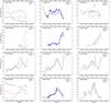 |
Fig. 2 Columns as in Fig. 1 for four additional sources, namely J1256-0547 (3C 279), J1504+1029 (PKS 1502+106), J1512-0905 (PKS 1510-089), and J2253+1608 (3C 454.3). |
3.1. Light curves and variability characteristics
Examples of combined EB/PV (2.6 to 228 GHz) light curves of active Fermi γ-ray sources are shown in Figs. 1 and 2; they show the variety of cm to short-mm band variability behaviours. Strong, correlated outbursts across the observing period are visible. These typically last from months to about one year and are seen in nearly all bands, often delayed and with lower variability amplitudes towards lower frequencies, e.g. in J0238+1636 (AO 0235+164) or J2253+1608 (3C 454.3). Often more fine structure, i.e. faster variability, is seen towards shorter wavelengths. In several cases, such as J1256-0547 (3C 279) and J2253+1608 (3C 454.3), there is very little or no variability in the lowest frequency bands (4.85 and 2.64 GHz). The case of J0359+5057 (NRAO 150) also demonstrates the presence of different variability properties with a nearly simultaneous, monotonic total flux density increase at all frequencies on much larger time scales (years). Interestingly, the latter happens without strong spectral changes (see also Sect. 3.7).
Figures 1 and 2 also include the denser sampled light curves obtained by the OVRO programme at 15 GHz. Even visual comparison shows the good agreement between the programmes. The EB data closely resemble the variability behaviour seen at higher time resolution with the OVRO 40 m data. To evaluate the agreement of the cross-station calibration we compared the EB and OVRO data sets at the nearby frequencies of 15 and 14.6 GHz. For the calibrators (non-variable steep spectrum sources) the difference is about 1.2% and can be accounted for by the source spectrum, given the slightly different central frequencies at EB and OVRO. Occasional divergence from this minor effect can be explained by pointing offsets and source spectral variability. Generally, the two stations agree within <3–4%.
To study the flare characteristics, a detailed light curve analysis was performed. For consistency we used the two-year data set, from June 2007 to June 2009, where quasi-simultaneous data from both EB and PV are available. The analysis included (i) a χ2-test for assessing the significance of the source variability; (ii) determination of the variability amplitude and its frequency dependence; and (iii) estimation of the observed flare time scales over the considered time period. Subsequently, multi-frequency variability brightness temperatures and Doppler factors are calculated. The analysis and results are discussed in the following sections.
3.2. Assessing the significance of variability
For each source and frequency, the presence of significant variability was examined under the hypothesis of a constant function and a corresponding χ2 test. A light curve is considered variable if the χ2 test gives a probability of ≤ 0.1% for the observed data under the assumption of constant flux density (99.9% significance level for variability).
The χ2 test results reveal that all primary (EB) and secondary (PV) calibrators are non-variable, as expected. The overall good calibration/gain stability is demonstrated by the small residual (mean) scatter (ΔS/⟨S⟩) in the calibrator light curves of 0.6 to 2.7% between 2.6 and 86.2 GHz, respectively. At 142.3 and 228.9 GHz, however, these values increase by a factor of up to 2–3. Almost all target sources of the F-GAMMA sample (for which the available data sets at the given frequency were sufficiently large) are variable across all bands. Taking all frequencies into account, we obtain a mean of 91% of target sources to be significantly variable at a 99.9% significance level. We note a trend of lower percentage of significantly variable sources (between 78 and 87%) at 43, 142.3, and 228.9 GHz. At these bands the measurement uncertainties are significantly higher owing to lower system performance and increasing influence of the atmosphere. Consequently, the larger measurement uncertainties at these bands reduce our sensitivity in detecting significant variability, particularly in the case of small amplitude variations and weaker sources. For subsequent analysis, only light curves exhibiting significant variability according to the χ2 test are considered.
3.3. Dependence of variability amplitudes on frequency
To quantify the strength of the observed flares in our light curves, we calculated the modulation index mν = 100 × σν/ ⟨Sν⟩ , where ⟨Sν⟩ is the mean flux density of the light curve at the given frequency and σν its standard deviation. The calculated modulation indices for each source and frequency show a clear trend. The sample’s averaged variability amplitude ⟨mν⟩ steadily increases towards higher frequencies from 9.5% at 2.6 GHz to 30.0% at 228.9 GHz. A similar behaviour is found in previous studies (e.g. Valtaoja et al. 1992; Ciaramella et al. 2004) though for smaller source samples, lower frequency coverage (typically up to 37 GHz), and different definitions of the variability amplitudes.
In order to establish this trend as an “intrinsic property”, possible biases in the calculated variability amplitudes have been taken into account as follows. First, owing to the dependence of the mean flux density ⟨Sν⟩ on frequency, we only consider the standard deviation of the flux density of each light curve as a measure of the mean variability/flare strength at a given frequency. Second, redshift effects are removed by converting to rest-frame frequencies. Finally, we remove the possible influence of measurement uncertainties (finite and different sampling, single-flux-density uncertainties) by computing intrinsic values for the flux density standard deviation of each light curve using a likelihood analysis. That is, assuming a Gaussian distribution of fluxes in each light curve, we compute the joint likelihood of all observations as a function of both the intrinsic mean flux density S0 and intrinsic standard deviation σ0, accounting for the different measurement uncertainties σj at each flux density measurement Sj, and the different number of flux density measurements for different light curves. The joint likelihood for N observations is (Richards et al. 2011, Eq. (20) with derivation therein) ![\begin{eqnarray} \mathcal{L}(S_0,\sigma_0) &=& \left( \prod_{j=1}^N \frac{1}{\sqrt{2\pi(\sigma_0^2 + \sigma_j^2)}}\right) \nonumber \\ && \quad \times \exp \left[-\frac{1}{2}\sum_{j=1}^N\frac{(S_j-S_0)^2}{\sigma_j^2 + \sigma_0^2}\right]\cdot \end{eqnarray}](/articles/aa/full_html/2016/12/aa28034-15/aa28034-15-eq27.png) (1)Marginalising out the intrinsic mean S0, we can obtain the maximum likelihood values for σ0, as well as uncertainties on this estimate. We consider a source to be variable at a given frequency if σ0 at that frequency is more than three sigma away from 0.
(1)Marginalising out the intrinsic mean S0, we can obtain the maximum likelihood values for σ0, as well as uncertainties on this estimate. We consider a source to be variable at a given frequency if σ0 at that frequency is more than three sigma away from 0.
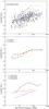 |
Fig. 3 Strength of variability (flux standard deviation) with respect to rest-frame frequency as observed with EB and PV. Top: Scatter plot (black, all sources) showing increasing variations with frequency. Superimposed are shown the logarithmic sample averages of the standard deviation after binning in frequency space. Middle: logarithmic averages of the standard deviation obtained for the FSRQs (red) and BL Lacs (green) in the sample. Bottom: three examples of individual sources showing (i) a rising trend (blue); (ii) a clear peak (black); and (iii) a nearly flat trend of variability amplitude across our bandpass (red). |
The results are summarised in Fig. 3, which shows the logarithmic flux standard deviations versus rest-frame frequency for each source, as well as the logarithmic sample averages per frequency bin. A clear and significant overall increase of the variability amplitude with increasing frequency is observed for the F-GAMMA sample, with a maximum reached at rest-frame frequencies ~60–80 GHz; i.e. the mm bands. At higher frequencies a plateau or a decreasing trend appears to be present, but cannot be clearly established owing to the small number of data points. Looking into individual source patterns, however, reveals three different behaviours: (i) sources showing only a rising trend towards higher frequencies; (ii) sources showing a clear peak at rest-frame frequencies between ~40–100 GHz with a subsequent decrease; and (iii) a few sources showing only a nearly flat trend across our bandpass. Typical examples are shown in the bottom panel of Fig. 3. Consequently, the high-frequency plateau in Fig. 3 (top) is the result of averaging over these different behaviours.
Detailed studies of single sources and isolated flares (e.g. Hovatta et al. 2008; Karamanavis et al. 2016a) at their different stages (maxima, slopes of the rising and decaying regimes; see Fig. 3) are required for detailed comparisons with model predictions (e.g. Fromm et al. 2015). However, the above findings (rising and peaking sources) are qualitatively in good agreement with predictions of shock-in-jet models (e.g. Marscher & Gear 1985; Valtaoja et al. 1992; Türler et al. 2000; Fromm et al. 2011, 2015) where the amplitude of flux variations is expected to follow three different regimes (growth at high frequencies, plateau, decay towards lower frequencies; see e.g. Valtaoja et al. 1992) according to the three stages of shock evolution (Compton, synchrotron, adiabatic loss phases; Marscher & Gear 1985). With good frequency coverage up to 375 GHz, Stevens et al. (1994) interpreted the overall flaring behaviour of their 17 sources, also in good agreement with the shock scenario with peaking variability amplitudes at ≤90 GHz, similar to our findings. Similar results have also been reported by Hovatta et al. (2008) using a large number of individual flares, and by Karamanavis et al. (2016a) for the broadband flare of PKS 1502+106.
In this framework, Fig. 3 demonstrates that the F-GAMMA frequency bands largely cover the decay stage of shocks, but also provide the necessary coverage towards higher frequencies to study the growth and plateau stages (peaking sources) and thus, test shock-in-jet models in detail (Angelakis et al. 2012; Fromm et al. 2015). Here, our APEX monitoring at 345 GHz will add important information to the initial shock formation/growth phase for a large number of sources. The origin of the nearly flat trend seen for some sources, however, needs particular investigation. Such behaviour is not easily understood within the standard shock scenario. The majority of these sources are also found to exhibit a different spectral behaviour (see Sect. 3.7).
Figure 3 (middle) shows the behaviour of the logarithmic average of the standard deviations with rest-frame frequency, for the FSRQs (red) and BL Lacs (green) in our sample. It is interesting to note that the FSRQs exhibit systematically higher variability amplitudes at lower frequencies (in contrast to e.g. the OVRO 15 GHz results; see below). However, this difference decreases at rest-frame frequencies ≳15 GHz and finally disappears at higher frequencies (≳20–30 GHz). This behaviour can be understood for BL Lacs showing stronger self-absorption and exhibiting flares largely decaying before reaching the lowest frequencies, which is in agreement with our spectral analysis (see Sect. 3.7).
We stress that previous studies found the opposite behaviour, i.e. BL Lacs exhibiting larger variability amplitudes than FSRQs at comparable frequencies (e.g. Ciaramella et al. 2004; Richards et al. 2011). In contrast to our measure of the variability amplitude (light curve standard deviations), these studies used the modulation index with the mean flux density as a normalisation factor. Although useful quantities for various studies, the normalisation leads only to apparently higher variability amplitudes for BL Lacs owing to the frequency-dependent, and on average lower, flux density of BL Lacs compared to FSRQs (in our sample by a factor 3–4).
3.4. Flare time scales
Under the assumption that the emission during outbursts arises from causally connected regions, the average rise and decay time of flares (i.e. their time scales, τvar) can constrain the size of the emitting region. Combined with the flare amplitude (Sect. 3.3), this information can yield physical parameters such as the brightness temperature and Doppler factor. To obtain τvar, and given the large number of data sets and flares to be analysed, we do not attempt to study individual flares, but instead use a structure function analysis (Simonetti et al. 1985). In particular, two different algorithms have been developed aiming at an automated estimation of flare time scales (see also Marchili et al. 2012).
The first applies a least-squares regression, of the form SF(τ) = const.·τα, to the structure function values at time lag τ. The regression is calculated over time lag windows of different size, providing a correlation coefficient for each. This method exploits the fact that, for time lags higher than the structure function plateau level, the correlation coefficient should undergo a monotonic decrease. Therefore, the observed time scale could be defined as the time lag τreg for which the coefficient regression is maximum. However, a change in the SF(τ) slope may cause a decrease in the regression coefficient before the plateau level is reached. Given the limited number of data points per light curve, such changes of slope often do not reflect a significant variability characteristic of the light curve. In order to overcome this problem, the time scale τc1 was defined as the first structure function maximum at time lags higher than τreg.
The structure function of a time series whose variability is characterised by a broken power-law spectrum shows a plateau after which it becomes almost flat. This is exploited by the second algorithm for the estimation of the time scale. Defining SFplateau as the structure function value at the plateau, we calculated τc2 as the lower time lag for which SF(τ) >SFplateau.
The use of automated procedures for the estimation of time scales considerably speeds it up and provides a fully objective and reproducible method. We compared the time scales obtained automatically with the ones resulting from visual inspection of the structure function as well as light curve plots for a sample of sources. The agreement between the results is satisfactory. If the difference | τc1−τc2 | is equal to or smaller than the average sampling of the investigated light curve, we considered the two values to be related to the same time scale, which is then defined as their average. Large discrepancies between the results of the two methods have been considered strong evidence of multiple time scales in the light curves. In this case, the two values have been considered separately. Occasionally, the estimated time scale coincides with the maximum time lag investigated by means of structure function. This occurs in cases where a (long-term) flare is just observed as a monotonic trend not changing throughout the whole time span of the observations. In these cases, the estimated time scale must be considered as a lower limit to the true flare time scale.
Mean and median variability parameters for different frequencies and source class.
The values returned by the structure function have been cross-checked by means of a wavelet-based algorithm for the estimation of time scales, based on the Ricker mother wavelet (a detailed discussion of this time analysis method can be found in Marchili et al. 2012). Given the fundamental differences between the structure function and wavelet algorithms for the estimation of time scales, the combined use of these two analysis tools is very effective for testing the reliability of the results. The substantial agreement between the two methods is demonstrated by a linear regression between their time scale estimates, which returns a correlation coefficient of ~ 0.8.
We note that our almost monthly cadence hampers the detection and investigation of more rapid flares (≲days to weeks), while the limited 2.5 yr time span of the current light curves sets an obvious limit to the maximum time scales that can be studied. Furthermore, the estimation of meaningful flare time scales at 228.9 GHz is strongly limited by the often much lower number of data points (see Figs. 1 and 2), large measurement uncertainties, and the reduced number of significantly variable sources (see Sect. 3.2). Consequently, we exclude the 228.9 GHz light curves from the current analysis.
The estimated time scales of the flares typically range between 80 and 500 days. The sample mean and median values obtained at each frequency are given in Table 3. A clear trend of faster variability towards higher frequencies is found with mean values of 348 days (median: 350 days), 294 days (median: 270 days), and 273 days (median: 240 days) at 2.6, 14.6, and 86.2 GHz, respectively. According to statistical tests (K-S test), no significant difference between FSRQs and BL Lacs is seen.
3.5. Variability brightness temperatures
Based on the variability parameters discussed above we obtain estimates of the emitting source sizes (via the light travel-time argument) and the variability brightness temperatures. Assuming a single emitting component with Gaussian brightness distribution, and given the redshift z, luminosity distance Dl, the estimated time scale τvar, and amplitude ΔS (~![\hbox{$\!\sqrt{0.5\cdot\rm{SF}\,[\tau]}$}](/articles/aa/full_html/2016/12/aa28034-15/aa28034-15-eq48.png) ) of variation, the apparent brightness temperature at frequency ν can be estimated as (e.g. Angelakis et al. 2015)
) of variation, the apparent brightness temperature at frequency ν can be estimated as (e.g. Angelakis et al. 2015) ![\begin{equation} T_{\mathrm{b,var}}\mathrm{[K]}=1.47\times10^{13}\Delta S\mathrm{[Jy]}\,\left[\frac{D_{\mathrm{l}}\,\mathrm{[Mpc]}}{\nu\,\mathrm{[GHz]} ~\tau_{\mathrm{var}}\,\mathrm{[days]}~(1+z)^2}\right]^2\cdot\label{tb1} \end{equation}](/articles/aa/full_html/2016/12/aa28034-15/aa28034-15-eq49.png) (2)The calculated values typically range between 109 and 1014 K. The distribution of Tb,var at different frequencies allows, for the first time, a detailed study of the frequency dependence of Tb,var across such a wide frequency range. Examples of variability brightness temperature distributions for selected frequencies are shown in Fig. 4, whereas the sample averaged, multi-frequency results are summarised in Table 3. We notice two main features:
(2)The calculated values typically range between 109 and 1014 K. The distribution of Tb,var at different frequencies allows, for the first time, a detailed study of the frequency dependence of Tb,var across such a wide frequency range. Examples of variability brightness temperature distributions for selected frequencies are shown in Fig. 4, whereas the sample averaged, multi-frequency results are summarised in Table 3. We notice two main features:
-
(i)
a systematic trend of decreasing Tb,var towards higher frequencies, by two orders of magnitude, with mean values of 4.0 × 10¹³ K (median: 1.3 × 10¹³ K), 3.7 × 10¹² K (median: 1.6 × 10¹² K), and 2.8 × 10¹¹ K (median: 1.0 × 10¹¹ K) at 2.6, 14.6, and 86.2 GHz, respectively;
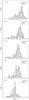
Fig. 4 Distributions of apparent variability brightness temperatures at selected frequencies: 2.64, 4.85, 14.6, 32, and 86 GHz from top to bottom. All sources (grey) are shown with FSRQs (black) and BL Lacs (green) superimposed. We note the systematic decrease of Tb,var towards higher frequencies as well as the difference in the sample between FSRQs and BL Lacs (see text).
-
(ii)
a difference between FSRQs and BL Lacs in our sample with a trend of higher brightness temperatures for FSRQs as compared to those of BL Lacs (see Table 3 and Fig. 4). A significant difference between the two classes in the sample is statistically confirmed at frequencies between 2.6 and 22 GHz by Kolmogorov-Smirnov (K-S) tests and Student’s t-tests, rejecting the null hypothesis of no difference between the two data sets (P< 0.001). Towards mm bands, however, this difference becomes less significant and vanishes at e.g. 86 GHz (see also Fig. 4).
3.6. Variability Doppler factors
Under equipartition between particle energy density and magnetic field energy density, a limiting brightness temperature  , of 5 × 10¹⁰ K is assumed (Scott & Readhead 1977; Readhead 1994; Lahteenmaki et al. 1999). We estimate the Doppler boosting factors by attributing the excess brightness temperature to relativistic boosting of radiation. The Doppler factor is then given by
 ![\hbox{$\delta_{\mathrm{var,eq}}=(1+z)\sqrt[3-\alpha]{T_{\mathrm{b}}/5\times 10^{10}}$}](/articles/aa/full_html/2016/12/aa28034-15/aa28034-15-eq62.png) (with α = −0.7; S ~ να). The sample averaged Doppler factors at each frequency are summarised in Table 3. Doppler factor distributions at different frequencies are shown in Fig. 5.
(with α = −0.7; S ~ να). The sample averaged Doppler factors at each frequency are summarised in Table 3. Doppler factor distributions at different frequencies are shown in Fig. 5.
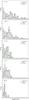 |
Fig. 5 Distributions of variability Doppler factors δvar,eq at selected frequencies: 2.64, 4.85, 14.6, 32, and 86 GHz from top to bottom. All sources (grey) are shown with FSRQs (black) and BL Lacs (green) superimposed. We note the systematic decrease of δvar,eq towards higher frequencies as well as the difference in the sample between FSRQs and BL Lacs (see text). |
Two main points can be made:
-
(i)
a systematic trend of decreasingδvar,eq towards higher frequencies by more than a factor of 4 with mean values of 8.8 (median: 8.2), 4.8 (median: 4.5), and 2.3 (median: 2.2) at 2.6, 14.6, and 86.2 GHz, respectively;
-
(ii)
a difference between FSRQs and BL Lacs in our sample with a trend of higher Doppler factors for FSRQs, as compared to those of BL Lacs, by a factor of 2–3 (see Table 3 and Fig. 5). Again, a significant difference between the two classes in the sample is statistically confirmed at frequencies between 2.6 and 22 GHz by K-S and Student’s t-tests rejecting the null hypothesis of no difference between the two data sets (P< 0.001). As seen from Fig. 5, the separation of the two sub-samples again vanishes towards the highest frequencies confirmed by accordingly higher K-S test values.
A trend of decreasing Tb,var and δvar,eq towards higher frequencies has already been reported (e.g. Fuhrmann et al. 2008; Karamanavis et al. 2016b; Lee et al. 2016). As pointed out by Lahteenmaki & Valtaoja (1999), maximum (intrinsic) brightness temperatures are expected to occur during the maximum development phase of shocks, i.e. at rest-frame frequencies of ~60–80 GHz (Sect. 3.3).
Our findings indicate that Tb,var is a decreasing function of frequency, as is also expected from the following considerations. Starting from Eq. (2)it is possible to write  (3)Assuming that the variability is caused by shocks travelling downstream, δS is expected to follow an increasing trend with ν within our bandpass (Valtaoja et al. 1992). From our data set (Fig. 3) we find that
  (4)On the other hand, δt is the time needed by the variability event to build the amplitude δS. This is related to the pace of evolution of the event. Using the mean time scales at each frequency for all sources, we find that
  (5)If we then substitute δt and δS in Eq. (3)we find that
 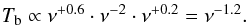 (6)Any divergence from this relation would require an alternative interpretation. The logarithm of the median brightness temperatures – for FSRQs – shown in Table 3, indeed follows an exponential drop with index − 1.17 ± 0.15, remarkably close to the expected value. The observed trend may suggest that the Doppler factors of blazars at cm and mm wavelengths are generally different – a scenario not unlikely for stratified and optically thick, self-absorbed, bent blazar jets. While probing a different jet region at each wavelength, each region may exhibit different Doppler factors depending on jet speed and/or viewing angle. Looking deeper into the jet towards higher frequencies, decreasing Doppler boosting would then indicate either increasing Lorentz factors along the jet or jet bending towards the observer for outward motion (with physical jet acceleration being statistically more likely). This interpretation is supported by the increasing evidence that individual VLBI components of blazar jets often show changes in apparent jet speed (e.g. Jorstad et al. 2005) with a significant fraction of these changes being due to changes in intrinsic speed (Homan et al. 2009). In the following, we briefly explore and discuss a few alternative explanations. For instance, another possibility to explain the observed Tb,var trend is an equipartition brightness temperature limit changing along the jet: might be different at different frequencies. In order to maintain constant Doppler boosting along the jet, for instance, should decrease towards higher frequencies. It must be noted that the relatively lower time sampling at higher frequencies could underestimate the variability time scales.
The observed trend of higher Tb,var and stronger Doppler boosting in FSRQs, as compared to BL Lacs, confirms earlier results (e.g. Lahteenmaki & Valtaoja 1999; Hovatta et al. 2008); however, here we demonstrate this effect at a much broader frequency range. Furthermore, this trend is in line with previous VLBI findings of BL Lacs exhibiting much slower apparent jet speeds and Lorentz factors as compared to those of FSRQs (e.g. Piner et al. 2010). The decreasing difference between FSRQs and BL Lacs (Tb,var and δvar,eq) towards higher frequencies, however, is in good agreement with the findings of Sects. 3.3 and 3.4; the higher variability amplitudes of FSRQs at lower frequencies result in correspondingly higher brightness temperatures and Doppler factors towards lower frequencies.
3.7. Spectral variability
The data obtained at EB and PV are combined to produce approximately monthly-sampled broadband spectra for each source. The maximum separation of measurements in a single spectrum is kept below 10 days. This span was chosen as a compromise between good simultaneity and the maximum number of combined EB/PV spectra. Specific sources may show detectable evolution already beyond 10 days.
In general, the sources show a variety of behaviours. The spectra of the example sources shown in Figs. 1 and 2 are presented in Fig. 6, giving a flavour of the different spectral behaviours observed. Often the flares seen in the light curves are accompanied by clear spectral evolution. Their spectral peaks νpeak occur first at the highest frequencies and successively evolve towards lower frequencies and lower flux densities. Typically, an evolving synchrotron self-absorbed component populating a low-frequency steep-spectrum component and unchanged component (quiescent, large-scale jet) is seen. However, the dominance and broadness of the steep-spectrum component, the lowest frequency reached by the flare component, and the relative strength of the two components differ from source to source.
The evolution of the flare components appears consistent with the predictions of the shock-in-jet model, that is, following the three-stage evolutionary path with Compton, synchrotron, and adiabatic loss phases in the “Sνpeak–νpeak” plane. Angelakis et al. (2012) showed that the plurality of the observed phenomenologies can be classified into only five variability classes. Except for the last type all other observed behaviours can be naturally explained with a simple two-component system composed of a steep quiescent spectral component from a large-scale jet and a time evolving flare component following the “shock-in-jet” evolutionary path like the one described before.
Several cases imply a different variability mechanism with only minor – if any – spectral evolution that does not seem to be described by the standard three-stage scenario. J0359+5057 (NRAO 150) in Fig. 6 is a typical example where almost no broadband spectral changes are observed during flux changes. In these cases, modifications of the shock-in-jet model or alternative variability models are required. Geometrical effects in helical, bent, or swinging jets (e.g. Villata & Raiteri 1999) can possibly be involved in the observed variability (see also e.g. Chen et al. 2013). Particularly in the case of NRAO 150, high-frequency VLBI observations indeed show the presence of a wobbling jet (Agudo et al. 2007).
 |
Fig. 6 Broadband radio spectra and spectral evolution of the sources shown in Figs. 1 and 2 combining the quasi-simultaneous multi-frequency data obtained at EB and PV. Angelakis et al. (2011, 2012) suggests a unification scheme for the variability patterns and a simple model that can reproduce all observed phenomenologies. |
3.8. Spectral index distribution
Here we examine the distribution of the multi-frequency spectral indices. We define the spectral index α as S ~ να with S the flux density measured at frequency ν. For each source we compute mean spectral indices by performing power law fits to averaged spectra. Three-point spectral indices have been obtained separately for the low sub-band at 4.85, 10.45, and 14.6 GHz and for the high sub-band at 32, 86.2, and 142.3 GHz. The distributions for the two sub-bands and FSRQ and BL Lacs sources separately, are shown in Fig. 7. The following can be seen there:
-
(i)
The low-frequency spectral index distribution is shown in theupper panel of Fig. 7. The mean over the wholesample, independent of source class (grey area), is − 0.03 with a median of − 0.05. The FSRQs (black line) show a mean of 0.02, but their distribution appears broadened with a tail towards more inverted spectra (median of − 0.03). The BL Lacs on the other hand (green line), give a mean of − 0.08 (median: − 0.1). Although their distribution appears shifted slightly towards steeper spectra than the FSRQs, a K-S test has not yielded any significant difference.
-
(ii)
The distribution of the upper sub-band spectral index (32, 86.2, and 142.3 GHz) is shown in the lower panel of Fig. 6. The mean over the entire sample is still − 0.03 (median: − 0.13), though the overall distribution now appears narrower. We note, however, a few sources contributing values >0.7, i.e. showing, on average, remarkably inverted spectra. The FSRQs in the sample now show a much narrower distribution which is interestingly skewed towards negative values with its mean at − 0.23 (median: − 0.25). The BL Lacs, however, concentrate around flatter or more inverted spectral indices (mean: 0.35). A K-S test indicates a significant difference between the two distributions (P < 0.001).
It must be emphasised that the overall flatness of the broadband radio spectra – expected for blazars and discussed above – is the result of averaging over a “evolving spectral components” through the observing bandpass.
The rather blurred picture seen in the low sub-band spectral index becomes slightly clearer at higher frequencies. The FSRQs clearly tend to concentrate around negative values contrary to the BL Lacs that concentrate around flat or inverted values. The broader scatter of the low-frequency spectral index is expected since at this regime where the observed emission is the superposition of slowly evolving past events. At higher frequencies where the evolution is faster, this degeneracy is limited. The divergence of the FSRQs and BL Lacs distributions can be understood by assuming that the latter show turnover frequencies at systematically higher frequencies or that their flares systematically do not reach the lowest frequencies in contrast to FSRQs. This may indicate different physical conditions in the two classes. However, this interpretation would also give a natural explanation for the trend of BL Lacs to show lower variability amplitudes (Sect. 3.3) towards lower frequencies.
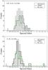 |
Fig. 7 Distributions of the mean spectral index over 2.5 yr of monitoring: top: low-frequency (4.85, 10.45, and 14.6 GHz) spectral index, bottom: high-frequency (32, 86.2, and 142.3 GHz) spectral index (see text). |
4. Radio variability and γ-ray loudness
The comparison of the F-GAMMA sample with the early Fermi AGN source list LBAS (Abdo et al. 2009c), showed that 29 of our 62 sources were detected in the first three months of operation confirming the initial source selection. After 11 months (Fermi 1LAC Catalog Abdo et al. 2010b) 54 of the 62 sources (i.e. 87%) were detected. As a result, the F-GAMMA programme participated in several multi-wavelength campaigns initiated by the Fermi team (e.g. 3C 454.3, 3C 279, PKS 1502+106, Mrk 421, Mrk 501, 3C 66A, AO 0235+164; Abdo et al. 2009a, 2010f,e, 2011a,b,c; Ackermann et al. 2012) and in broadband studies of larger samples (Abdo et al. 2010a; Giommi et al. 2012). See Fuhrmann (2010) for an overview of the early campaigns.
In the following we examine whether the radio variability triggers the source γ-ray activity and subsequently their Fermi detectability.
4.1. Radio variability amplitude and Fermi detectability
In this section we examine whether radio variability – expressed by the standard deviation of the flux density – is correlated with γ-ray loudness of the sources. In this context the proxy for the γ-ray loudness is the source Fermi early detectability.
Such a correlation would agree with findings that indicate that γ-ray flares often occur during high-flux radio states (e.g. Kovalev et al. 2009; León-Tavares et al. 2011; Fuhrmann et al. 2014). A connection between the variability amplitude in the radio (quantified by the intrinsic modulation index) and the γ-ray loudness inferred from the source presence in the 1LAC Catalog, has been confirmed with high significance by Richards et al. (2011) using 15 GHz OVRO data. Here, we examine whether such a connection persists in the F-GAMMA data, and how frequency affects such a connection. Instead of the modulation index we use the flux density standard deviation.
Figure 8 shows the dependence of the logarithmic average of the flux density standard deviation on the rest-frame frequency. Sources included in one of the first Fermi catalogues are plotted separately from those not included. The upper panel refers to the LBAS and the lower panel to the 1LAC Catalog. In the first case, the two curves appear clearly separated. The γ-ray detected sources display larger variability amplitudes confirming our expectations. On average they are more than a factor of 3 more variable at the highest frequencies where the largest separation is seen. The same conclusion is reached when the 1LAC is used as a reference. In this case the statistics are not as good (fewer F-GAMMA sources are absent from the 1LAC) as it is imprinted in the larger error bars in the logarithmic mean. Finally, it is worth noting a clear increase in the separation between the two curves towards higher frequencies. This further supports our findings that the radio/γ-ray correlation becomes stronger towards higher frequencies both at the level of average fluxes (see Sect. 5) and at the level of light curve cross-correlations for which smaller time lags are found (Fuhrmann et al. 2014).
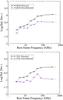 |
Fig. 8 Variability amplitude against rest-frame frequency for the Fermi LBAS detected/non-detected sources (upper panel) and 1FGL detected/non-detected sources (lower panel) of the F-GAMMA sample. y-axis: logarithmic average of the light curve standard deviations |
4.2. Brightness temperatures and Doppler factors versus Fermi detectability
We also investigate possible differences between the observed variability time scales, variability brightness temperatures, and Doppler factors of Fermi-detected and non-detected sources in our sample.
Although no real differences were in the variability time scale, there is a clear trend of the Fermi-detected sources (LBAS and 1LAC) to show variability brightness temperatures that are higher by a factor of ~2–3. The effect is noticeable is all our radio bands. At 86.2 GHz for example, the LBAS sources show a mean TB,var of 4.0 × 10¹¹ K (median: 9.9 × 10¹⁰ K), whereas the non-LBAS sources exhibit a mean of 1.6 × 10¹¹ K (median: 9.6 × 10¹⁰ K). Given our previous discussion that Fermi-detected sources show larger variability amplitudes (Sect. 4.1), such a trend is expected owing to the dependence of the variability brightness temperature to the variability amplitude (Eq. (2)).
We also note a trend of slightly higher variability Doppler factors δvar,eq for the Fermi-detected sources across all radio bands. This is in agreement with previous findings of Savolainen et al. (2010) reporting larger variability Doppler factors of Fermi-detected sources based on Metsähovi long-term light curves.
In contrast to Savolainen et al. (2010), however, the above-mentioned difference between Fermi-detected and non-detected sources in terms of TB,var and δvar,eq cannot be established with a high statistical significance. It is likely that this is an effect of the limited data set discussed here and of the method used for the estimation of δvar,eq, which relies on average time scales as opposed to time scales of the sharpest, fastest flares in the light curves.
5. Radio and γ-ray flux correlation
In this section we examine whether an intrinsic correlation between the radio and the γ-ray fluxes of sources in our sample exists. This would imply the physical connection between the emission region and emission processes in the two bands.
Strong correlations were previously claimed on the basis of EGRET data (e.g. Stecker et al. 1993; Padovani et al. 1993; Stecker & Salamon 1996), and were re-examined with more detailed statistical analyses (e.g. Muecke et al. 1997; Chiang & Mukherjee 1998). However, a number of effects make such correlations uncertain, and very careful treatment is necessary:
-
1.
in small samples with limited luminosity dynamic ranges,artificial flux-flux correlations may be induced by the commondistance effect;
-
2.
artificial luminosity-luminosity correlations can emerge when considering objects in flux-limited surveys. In such cases most objects are close to the survey sensitivity limit and by applying a common redshift to transfer to the luminosity space, artificial correlations appear;
-
3.
the data used to obtain the claimed correlations are not synchronous.
With the large number of Fermi-detected sources the correlations between radio and γ rays have been revisited over a broad range of radio data (e.g. Kovalev et al. 2009; Ghirlanda et al. 2010, 2011; Mahony et al. 2010). Ackermann et al. (2011a) used 8 GHz archival data for the largest sample ever used in such studies with 599 sources, and also used a smaller sample of concurrent 15 GHz measurements from the OVRO monitoring programme. They assessed the intrinsic significance of the observed correlations using the data randomisation technique of Pavlidou et al. (2012). They confirm a highly significant correlation between radio and γ-ray fluxes which becomes more significant when concurrent rather than archival radio data are used.
The F-GAMMA data set can provide new insight into the problem by taking the following into consideration:
-
the broad frequency range allows us to examine whether thesignificance and the parameters of the correlation show anyfrequency dependence (see Ackermannet al. 2011a, for a study of thisdependence on γ-ray photon energy);
-
our data are perfectly concurrent with measurements of γ-ray fluxes eliminating biases emerging from the non-simultaneity of observations;
-
the F-GAMMA data provide concurrent information of the radio spectral index, which is an essential input for the assessment of the significance of the correlations (Pavlidou et al. 2012).
On the other hand, there are certain features of our data sets that require a particularly careful treatment. First, the sources do not constitute a flux-limited sample. Although this makes them less sensitive to artificially induced luminosity-luminosity correlations (Malmquist bias), it also means that statistical tests usually employed to assess correlation significance cannot be benchmarked in a straightforward way by sampling the luminosity function (e.g. Bloom 2008). As a result, we need a specialised treatment to estimate how likely it is that a simple calculation of the correlation coefficient will overestimate the significance of an intrinsic correlation between radio and γ-ray fluxes owing to common-distance biases, and to calculate the intrinsic correlation significance.
5.1. Common-distance bias introduced by the limited dynamic range
As is shown in Pavlidou et al. (2012), there is a quantitative criterion that can be applied to determine the extent to which common-distance bias affects the correlation significance estimated for a specific data set using only the value for the correlation coefficient.
The bias is larger for samples with a small luminosity dynamic range, and a large redshift range. Conversely, samples with a large luminosity dynamic range compared to their redshift dynamical range are relatively robust against common-distance biases. This can be immediately understood in the limit where all the sources are at the same redshift, in which case there is no common-distance bias.
The quantity summarising the relative extent of the luminosity and redshift dynamic ranges of a sample is the ratio of the variation coefficient c of the luminosity and redshift distributions. This is defined as the standard deviation in units of the mean. Pavlidou et al. (2012) found that values of cL/cz smaller than 5 indicate that common-distance biases are important and can lead to a significant overestimation of the significance of a correlation between fluxes in two bands if only the correlation coefficient is used without appropriate Monte Carlo testing.
Table 4 shows the correlation coefficient for the logarithm of radio and γ-ray fluxes for each of our samples (corresponding to a specific radio frequency). As an illustration, the radio and γ-ray fluxes are plotted against each other in logarithmic axes for the cases of the 228.9, 86.2, and 10.45 GHz samples in Fig. 9.
Flux-flux correlation analysis: Monte Carlo results obtained for the different frequencies.
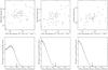 |
Fig. 9 Top: radio flux against Fermi γ-ray flux at 10.45 GHz (left), 86.2 GHz (middle), and 228.9 GHz (right) for the sources in our sample with known redshifts. Bottom: distribution of permutations-evaluated r-values (see text) for Fermi vs. 10.45 GHz (left), 86.2 GHz (middle), and 228.9 GHz (right) fluxes. Arrows indicate the r-values obtained for the actual data. |
As we can see in Table 4, there is a general trend for the correlation coefficient r to be high at high frequencies (r ~ 0.5 for 228.9 to 86.2 GHz), and significantly lower at lower frequencies (r < 0.4 at ν ≤ 43 GHz). However, these results cannot be taken at face value without appropriate statistical assessment, because cL/cz is smaller than 5 for both γ-ray and radio frequencies for all of our samples.
5.2. Treating the limited dynamic range
To address the peculiarities discussed above Pavlidou et al. (2012) developed a data randomisation method which is based only on permutations of the observed data. The method preserves the observed luminosity and flux density dynamic ranges and, provided the sample is large enough, also the observed luminosity, flux density, and redshift distributions. The technique has been designed to perform well even for samples selected in a subjective fashion, and it has been demonstrated that it never overestimates the correlation significance, while at the same time retaining the power of traditionally employed methods to establish a correlation when one indeed exists.
In brief, the method was applied as follows (see Pavlidou et al. 2012, for details):
-
1.
moving to luminosity space using the known redshifts and therelation between monochromatic flux densitySν and luminosity Lν. The simultaneously measured radio spectral indices (Sect. 3.7) allow us to concurrently perform a K-correction and calculate Lν at rest-frame frequency ν0 according to
 (7)where
  d
d . In the case of γ-ray observations the actual observed quantity is F, the photon flux integrated over energy from E0 = 1 GeV to ∞. This is related to monochromatic energy flux through Sγ = (α−1) F, where α is the absolute value of the photon spectral index. The obtained sets of radio and γ-ray luminosities fix our luminosity dynamical range;
 -
2.
constructing simulated fluxes in radio and γ-ray by combining each luminosity with one of the redshifts. Fluxes outside the original flux range are rejected as a single very high flux or very low flux and a cluster of points of similar fluxes can produce an artificially high correlation index, which would not occur given the original flux dynamical range;
-
3.
pairing up the accepted simulated fluxes in all possible combinations excluding the “true” flux pairs;
-
4.
selecting a large number (~107) of N pair combinations, where N is equal to the number of the original observations. Each set of N pairs is a set of uncorrelated simulated flux observations;
-
5.
computing the Pearson product-moment correlation coefficient r for each simulated data set;
-
6.
performing steps 2 to 5 – provided the sample size is large enough – in redshift bins to limit the rejection of flux values and to maintain the luminosity and redshift distributions of the original sample (the sample size requirement is to have ≳10 sources in each bin).
5.3. Results of our analysis
The results of the previous analysis are shown in Table 4. The probability distributions of the Pearson product-moment correlation coefficient r for the simulated samples with intrinsically uncorrelated luminosities are given in Fig. 9. Arrows indicate the r-values obtained for the actual data as given in Table 4.
Radio frequencies at 43 GHz and above have a significant correlation with γ rays; better than 2σ and, in the case of 142.3 and 86.2 GHz, better than 3σ. Lower frequencies on the other hand never exceeded 2σ significance level. These suggest:
-
1.
A physical connection between the radio and high-energyemission. In the presence of a low-energy synchrotron photonfield, relativistic electrons and Doppler boosting, such acorrelation is expected in a scenario, where the high-energyemission is produced by inverse-Compton (IC) up-scattering offof low-energy synchrotron photons.
-
2.
The closer connection of the high radio frequency and IC γ-ray emitting regions. This is expected owing to lower intrinsic opacity at mm bands (e.g. Fuhrmann et al. 2014).
The applicability of this result must be appropriately qualified in the light of two specific concerns. First, because our sample is selected with subjective criteria, the result cannot be generalised to the blazar population. Instead it is only valid for the specific sources in our sample.
Second, lack of evidence for a significant correlation between low radio (<43 GHz) and γ-ray fluxes is not equivalent with evidence for lack of a positive correlation. A characteristic counter-example is our findings at 14.6 GHz. Although no significant correlation was found with our data, a positive correlation has been established at the same frequency for the Fermi-detected sub-set of CGRaBS (Ackermann et al. 2011a; Pavlidou et al. 2012) using OVRO 15 GHz data. The reason for this discrepancy is not the size of the sample, but rather the different makeup of the two samples. There are only 15 sources that are common to the two samples. Most of the additional sources in our sample are BL Lacs, while the OVRO sample is generally dominated by FSRQs. Ackermann et al. (2011a) treated BL Lacs and FSRQs separately and found that the correlation between Fermi and OVRO fluxes for BL Lacs was weak. It is only natural then that the F-GAMMA sample at 14.6 GHz showed a weak correlation owing to the dominance of BL Lacs.
The last two columns of Table 4 show the significances calculated using the high (φhigh) and low (φlow) spectral index discussed in Sect. 3.8. The radio spectral index has a mild effect on the calculation of the significance. We conclude then that the statistical method applied is robust even against small changes of the radio spectral index.
Finally, we have tested whether the time duration of integration affects the strength and the significance of the correlation between radio and γ-ray fluxes. For the 28 sources common in our 86.2 GHz sample, the LBAS and 1FGL, we have calculated the correlation coefficient r and the significance of the correlation between 86.2 GHz and 1 GeV flux densities averaged over three months and one year, the time spans relevant for LBAS and 1FGL, respectively. In the first case (LBAS) we found that r = 0.5 and p-value of 5.9 × 10⁻³. In the second case (1LAC), we found that r = 0.44 with a significance of 4.3%. We conclude that the correlation weakens when the averaging is extended over significantly longer time periods (~a year). Since the typical flaring event duration in radio is a few months, and assuming that over short γ-ray integrations it is typically the flaring sources that are detected, this effect may be an indication that there is a common origin between GeV flares and flares at high radio frequencies.
6. Summary and conclusions
We have presented the Fermi dedicated blazar radio multi-frequency monitoring programme, F-GAMMA. The F-GAMMA programme conducted a monthly monitoring of the radio variability and spectral evolution of ~60 γ-ray blazars at 12 frequencies between 2.6 and 345 GHz. The observations were carried with the Effelsberg 100 m, IRAM 30 m and APEX 12 m telescopes including polarisation at several bands. The initial sample presented here has been selected from the most prominent, frequently active, and bright blazars at δ ≥ −30°. The conclusions of the first 2.5 yr of analysis can be summarised as follows:
-
Our analysis shows that almost all sources are variable across allfrequency bands. On the basis of a maximum likelihood analysisthat accounts for possible biases, we have demonstrated that thevariability amplitude increases with increasing frequency up torest-frame frequencies of ~60–80 GHz; above this level the variability decreases or remains constant. The variability of individual sources, however, can rise continuously across or peak within our band. These findings agree with predictions of shock-in-jet models where the maximum amplitude of flux variations is expected to follow the standard growth, plateau, and decay phase.
-
At lower frequencies the FSRQs in our sample show larger variability amplitudes than BL Lacs – in terms of flux density variance – in contrast to previous findings that used variance in units of mean flux density. The discrepancy arises from the frequency dependence of the flux density, which for BL Lacs is on average significantly lower. This leads to apparently larger variability amplitudes for BL Lacs when the mean flux density is used for the normalisation of the variance.
-
The variability time scales range from 80 and 500 days depending on source and frequency. A clear trend of faster variability towards higher frequencies is observed. As an example, mean values of 348, 294, and 273 days at 2.64, 14.6, and 86.2 GHz, respectively, have been measured.
-
The calculated Tb,var values depend on frequency. They typically range from 109 to 1014 K. A systematic trend of decreasing Tb,var (by two orders of magnitudes) and δvar,eq (by more than a factor of 4) towards higher frequencies is observed with mean values for δvar,eq of e.g. 8.8, 4.8, and 2.3 at 2.64, 14.6, and 86.2 GHz, respectively.
-
The combination of EB and PV data sets provide a large data base of monthly sampled broadband spectra. Their time coherence is kept at 10 days and below. Typically, an evolving synchrotron self-absorbed component over a low-frequency steep-spectrum component (quiescent jet) is observed. Often the spectra follow the standard three-stage evolutionary path of shock. A physically different mechanism appears likely for several sources that display a nearly achromatic variability. The spectral evolution can also explain naturally the general flatness of the spectra (mean spectral index − 0.03 at low and high frequencies). The spectral flatness results naturally from averaging over different spectral components and their evolution across the spectrum over the 2.5-yr period.
-
We find significant differences between the FSRQs and BL Lacs in our sample. The BL Lacs show systematically smaller variability amplitudes at lower frequencies. The difference vanishes at higher frequencies. Although the variability time scales appear similar, the variability brightness temperatures and Doppler factors are also lower at lower frequencies for BL Lacs. The difference again decreases towards higher frequencies. This behaviour can be understood in the light of our spectral findings. For BL Lacs the high-frequency spectral indices are flatter or more inverted. This implies that flares appearing in BL Lacs show higher turn-over frequencies and that they systematically do not reach the lowest bands. Subsequently, they invoke lower variability amplitudes, lower Tb,var and lower δvar,eq values at these bands.
-
We searched for possible correlations of radio characteristics with γ-ray loudness. As a proxy we used the presence of the sources the LBAS and 1LAC catalogues. We find that the Fermi-detected sources show larger variability amplitudes than non-detected ones. The clear increase in the separation between flux standard deviation averages with increasing frequency supports an arguably tighter correlation between γ rays and higher radio bands. We also find a trend of higher Tb,var and δvar,eq in Fermi-detected sources.
-
We searched for correlations between F-GAMMA flux densities and concurrent Fermi/LAT 1 GeV fluxes for frequencies even up to 228.9 GHz. After a careful treatment of the limited dynamic ranges of our sample, we find that flux densities at ν ≥ 43 GHz correlate with 1 GeV fluxes at a significance level of better than 2σ; at 142.3 and 86.2 GHz the significance is better than 3σ. This implies that the γ-ray emission is produced very close to the mm-band emission region. This view is also supported by the fact that at 86.2 GHz flux densities averaged over a few months (comparable to the duration of a single flare) correlate at higher significance than flux densities averaged over longer time scales (a year, as in the 1LAC Catalog).
A five-year data analysis based on the revised F-GAMMA sample will be presented in a subsequent publication. Nestoras et al. (2016) discuss the first five years of PV data. Angelakis et al. (2012) studied the variability of the radio broadband spectra. They proposed that the variability patterns can be classified in only two categories, those showing intense spectral evolution and those that vary achromatically. They show that the former can be easily reproduced with simply the superposition of a steep-spectrum steady state component and a high-frequency component that evolves in time and frequency. For the γ-ray emission site, Fuhrmann et al. (2014) conducted a cross-correlation analysis between mm-radio and γ rays. They found that the γ-ray emission for 3C 454.3 originates at a distance of at least 0.8–1.6 pc from the supermassive black hole. Karamanavis et al. (2016b) examined the structural evolution of PKS 1502+106 during a γ-ray outburst with mm-VLBI. Using F-GAMMA data they estimated that the γ-ray emission site must be no farther than ~6 pc from the jet base. Later Karamanavis et al. (2016a) localised the emission site at 1.9 ± 1.1 pc from the jet base. Myserlis et al. (2014) looked at the multi-frequency linear and circular polarisation data to interpret rotations of the polarisation angle in terms of an opacity evolution effect. Liodakis et al. (2016) study the variability Doppler factors for EB and PV data and compare them with the predictions of blazar population models.
Acknowledgments
The authors would like to thank the anonymous referee for the very careful reading of the manuscript, and the constructive and insightful comments. They have noticeably improved the quality of the paper. We would also like to thank the MPIfR internal referees Drs J. Hodgson and C. Casadio for the careful reading of the manuscript. This research is based on observations with the 100 m telescope of the MPIfR (Max-Planck-Institut für Radioastronomie) at Effelsberg. It has also made use of observations with the IRAM 30 m telescope. IRAM is supported by INSU/CNRS (France), MPG (Germany), and IGN (Spain). I.N., V.K., and I.M. were funded by the International Max Planck Research School (IMPRS) for Astronomy and Astrophysics at the Universities of Bonn and Cologne. The OVRO 40 m programme is supported in part by NASA grants NNX08AW31G and NNG06GG1G and NSF grant AST-0808050. We would like to acknowledge partial support from the EU FP7 Grant PIRSES- GA-2012-316788.
References
- Abdo, A. A., Ackermann, M., Ajello, M., et al. 2009a, ApJ, 699, 817 [NASA ADS] [CrossRef] [Google Scholar]
- Abdo, A. A., Ackermann, M., Ajello, M., et al. 2009b, ApJ, 700, 597 [NASA ADS] [CrossRef] [Google Scholar]
- Abdo, A. A., Ackermann, M., Ajello, M., et al. 2009c, ApJ, 700, 597 [NASA ADS] [CrossRef] [Google Scholar]
- Abdo, A. A., Ackermann, M., Agudo, I., et al. 2010a, ApJ, 716, 30 [NASA ADS] [CrossRef] [Google Scholar]
- Abdo, A. A., Ackermann, M., Ajello, M., et al. 2010b, ApJS, 188, 405 [NASA ADS] [CrossRef] [Google Scholar]
- Abdo, A. A., Ackermann, M., Ajello, M., et al. 2010c, ApJ, 715, 429 [NASA ADS] [CrossRef] [Google Scholar]
- Abdo, A. A., Ackermann, M., Ajello, M., et al. 2010d, ApJ, 722, 520 [NASA ADS] [CrossRef] [Google Scholar]
- Abdo, A. A., Ackermann, M., Ajello, M., et al. 2010e, ApJ, 710, 810 [NASA ADS] [CrossRef] [Google Scholar]
- Abdo, A. A., Ackermann, M., Ajello, M., et al. 2010f, Nature, 463, 919 [NASA ADS] [CrossRef] [PubMed] [Google Scholar]
- Abdo, A. A., Ackermann, M., Ajello, M., et al. 2011a, ApJ, 727, 129 [NASA ADS] [CrossRef] [Google Scholar]
- Abdo, A. A., Ackermann, M., Ajello, M., et al. 2011b, ApJ, 736, 131 [NASA ADS] [CrossRef] [Google Scholar]
- Abdo, A. A., Ackermann, M., Ajello, M., et al. 2011c, ApJ, 726, 43 [NASA ADS] [CrossRef] [Google Scholar]
- Ackermann, M., Ajello, M., Allafort, A., et al. 2011a, ApJ, 741, 30 [NASA ADS] [CrossRef] [Google Scholar]
- Ackermann, M., Ajello, M., Allafort, A., et al. 2011b, ApJ, 743, 171 [NASA ADS] [CrossRef] [Google Scholar]
- Ackermann, M., Ajello, M., Ballet, J., et al. 2012, ApJ, 751, 159 [NASA ADS] [CrossRef] [Google Scholar]
- Ackermann, M., Ajello, M., Atwood, W. B., et al. 2015, ApJ, 810, 14 [NASA ADS] [CrossRef] [Google Scholar]
- Agudo, I., Bach, U., Krichbaum, T. P., et al. 2007, A&A, 476, L17 [NASA ADS] [CrossRef] [EDP Sciences] [Google Scholar]
- Agudo, I., Thum, C., Gómez, J. L., & Wiesemeyer, H. 2014, A&A, 566, A59 [NASA ADS] [CrossRef] [EDP Sciences] [Google Scholar]
- Aller, H. D. 1970, ApJ, 161, 1 [NASA ADS] [CrossRef] [Google Scholar]
- Aller, H. D., Aller, M. F., Latimer, G. E., & Hodge, P. E. 1985, ApJS, 59, 513 [NASA ADS] [CrossRef] [Google Scholar]
- Angelakis, E., Fuhrmann, L., Nestoras, I., et al. 2010, ArXiv e-prints [arXiv:1006.5610] [Google Scholar]
- Angelakis, E., Fuhrmann, L., Nestoras, I., et al. 2011, 2011 Fermi Symp. Proc., eConf. C110509 [arXiv:1111.6992] [Google Scholar]
- Angelakis, E., Fuhrmann, L., Nestoras, I., et al. 2012, J. Phys. Conf. Ser., 372, 012007 [NASA ADS] [CrossRef] [Google Scholar]
- Angelakis, E., Fuhrmann, L., Marchili, N., et al. 2015, A&A, 575, A55 [NASA ADS] [CrossRef] [EDP Sciences] [Google Scholar]
- Angelakis, E., Hovatta, T., Blinov, D., et al. 2016, MNRAS, 463, 3365 [NASA ADS] [CrossRef] [Google Scholar]
- Atwood, W. B., Abdo, A. A., Ackermann, M., et al. 2009, ApJ, 697, 1071 [NASA ADS] [CrossRef] [Google Scholar]
- Baars, J. W. M., Genzel, R., Pauliny-Toth, I. I. K., & Witzel, A. 1977, A&A, 61, 99 [NASA ADS] [Google Scholar]
- Bach, U., Raiteri, C. M., Villata, M., et al. 2007, A&A, 464, 175 [NASA ADS] [CrossRef] [EDP Sciences] [Google Scholar]
- Begelman, M. C., Blandford, R. D., & Rees, M. J. 1980, Nature, 287, 307 [NASA ADS] [CrossRef] [Google Scholar]
- Bennett, C. L., Hill, R. S., Hinshaw, G., et al. 2003, ApJS, 148, 97 [NASA ADS] [CrossRef] [Google Scholar]
- Blandford, R. D., & Königl, A. 1979, ApJ, 232, 34 [NASA ADS] [CrossRef] [Google Scholar]
- Blandford, R. D., & Levinson, A. 1995, ApJ, 441, 79 [NASA ADS] [CrossRef] [Google Scholar]
- Blandford, R. D., & Rees, M. J. 1974, MNRAS, 169, 395 [NASA ADS] [CrossRef] [Google Scholar]
- Blinov, D., Pavlidou, V., Papadakis, I., et al. 2015, MNRAS, 453, 1669 [NASA ADS] [CrossRef] [Google Scholar]
- Blinov, D., Pavlidou, V., Papadakis, I. E., et al. 2016, MNRAS, 457, 2252 [NASA ADS] [CrossRef] [Google Scholar]
- Bloom, S. D. 2008, ApJ, 136, 1533 [Google Scholar]
- Böttcher, M. 2007, Astrophys. Space Sci., 309, 95 [Google Scholar]
- Camenzind, M., & Krockenberger, M. 1992, A&A, 255, 59 [NASA ADS] [Google Scholar]
- Carrara, E. A., Abraham, Z., Unwin, S. C., & Zensus, J. A. 1993, A&A, 279, 83 [NASA ADS] [Google Scholar]
- Chen, X., Rachen, J. P., López-Caniego, M., et al. 2013, A&A, 553, A107 [NASA ADS] [CrossRef] [EDP Sciences] [Google Scholar]
- Chiang, J., & Mukherjee, R. 1998, ApJ, 496, 496, 752 [NASA ADS] [CrossRef] [Google Scholar]
- Ciaramella, A., Bongardo, C., Aller, H. D., et al. 2004, A&A, 419, 485 [NASA ADS] [CrossRef] [EDP Sciences] [Google Scholar]
- Cohen, M. H., Cannon, W., Purcell, G. H., et al. 1971, ApJ, 170, 207 [NASA ADS] [CrossRef] [Google Scholar]
- Dent, W. A. 1966, ApJ, 144, 843 [NASA ADS] [CrossRef] [Google Scholar]
- Dermer, C. D., Schlickeiser, R., & Mastichiadis, A. 1992, A&A, 256, L27 [NASA ADS] [Google Scholar]
- Fromm, C. M., Perucho, M., Ros, E., et al. 2011, A&A, 531, A95 [NASA ADS] [CrossRef] [EDP Sciences] [Google Scholar]
- Fromm, C. M., Fuhrmann, L., & Perucho, M. 2015, A&A, 580, A94 [NASA ADS] [CrossRef] [EDP Sciences] [Google Scholar]
- Fuhrmann, L. 2010, ArXiv e-prints [arXiv:1007.0348] [Google Scholar]
- Fuhrmann, L., Zensus, J. A., Krichbaum, T. P., Angelakis, E., & Readhead, A. C. S. 2007, in The First GLAST Symposium, eds. S. Ritz, P. Michelson, & C. A. Meegan, AIP Conf. Ser., 921, 249 [Google Scholar]
- Fuhrmann, L., Krichbaum, T. P., Witzel, A., et al. 2008, A&A, 490, 1019 [NASA ADS] [CrossRef] [EDP Sciences] [Google Scholar]
- Fuhrmann, L., Larsson, S., Chiang, J., et al. 2014, MNRAS, 441, 1899 [NASA ADS] [CrossRef] [Google Scholar]
- Ghirlanda, G., Ghisellini, G., Tavecchio, F., & Foschini, L. 2010, MNRAS, 407, 791 [NASA ADS] [CrossRef] [Google Scholar]
- Ghirlanda, G., Ghisellini, G., Tavecchio, F., Foschini, L., & Bonnoli, G. 2011, MNRAS, 413, 852 [NASA ADS] [CrossRef] [Google Scholar]
- Giommi, P., Polenta, G., Lähteenmäki, A., et al. 2012, A&A, 541, A160 [NASA ADS] [CrossRef] [EDP Sciences] [Google Scholar]
- Guetta, D., Ghisellini, G., Lazzati, D., & Celotti, A. 2004, A&A, 421, 877 [NASA ADS] [CrossRef] [EDP Sciences] [Google Scholar]
- Hargrave, P. J., & Ryle, M. 1974, MNRAS, 166, 305 [NASA ADS] [CrossRef] [Google Scholar]
- Hartman, R. C., Bertsch, D. L., Fichtel, C. E., et al. 1992, ApJ, 385, L1 [NASA ADS] [CrossRef] [Google Scholar]
- Hartman, R. C., Bertsch, D. L., Bloom, S. D., et al. 1999, ApJSS, 123, 79 [NASA ADS] [CrossRef] [Google Scholar]
- Healey, S. E., Romani, R. W., Cotter, G., et al. 2008, ApJS, 175, 97 [NASA ADS] [CrossRef] [Google Scholar]
- Homan, D. C., Kadler, M., Kellermann, K. I., et al. 2009, ApJ, 706, 1253 [NASA ADS] [CrossRef] [Google Scholar]
- Hovatta, T., Nieppola, E., Tornikoski, M., et al. 2008, A&A, 485, 51 [NASA ADS] [CrossRef] [EDP Sciences] [Google Scholar]
- Jorstad, S. G., Marscher, A. P., Mattox, J. R., et al. 2001, ApJ, 556, 738 [NASA ADS] [CrossRef] [Google Scholar]
- Jorstad, S. G., Marscher, A. P., Lister, M. L., et al. 2005, AJ, 130, 1418 [NASA ADS] [CrossRef] [Google Scholar]
- Karamanavis, V., Fuhrmann, L., Angelakis, E., et al. 2016a, A&A, 590, A48 [NASA ADS] [CrossRef] [EDP Sciences] [Google Scholar]
- Karamanavis, V., Fuhrmann, L., Krichbaum, T. P., et al. 2016b, A&A, 586, A60 [NASA ADS] [CrossRef] [EDP Sciences] [Google Scholar]
- King, O. G., Blinov, D., Ramaprakash, A. N., et al. 2014, MNRAS, 442, 1706 [NASA ADS] [CrossRef] [Google Scholar]
- Kovalev, Y. Y., Aller, H. D., Aller, M. F., et al. 2009, ApJ, 696, L17 [NASA ADS] [CrossRef] [Google Scholar]
- Kovalev, Y. Y., Kovalev, Y. A., Nizhelsky, N. A., & Bogdantsov, A. B. 2002, PASA, 19, 83 [NASA ADS] [CrossRef] [Google Scholar]
- Lahteenmaki, A., & Valtaoja, E. 1999, ApJ, 521, 493 [NASA ADS] [CrossRef] [Google Scholar]
- Lahteenmaki, A., Valtaoja, E., & Wiik, K. 1999, ApJ, 511, 112 [NASA ADS] [CrossRef] [Google Scholar]
- Larsson, S., Fuhrmann, L., Weiss, A., et al. 2012, 2012 Fermi & Jansky Proc., eConf C1111101 [arXiv:1206.3799] [Google Scholar]
- Lee, S.-S., Byun, D.-Y., Oh, C. S., et al. 2011, PASP, 123, 1398 [NASA ADS] [CrossRef] [Google Scholar]
- Lee, S.-S., Lobanov, A. P., Krichbaum, T. P., & Zensus, J. A. 2016, ApJ, 826, 135 [Google Scholar]
- León-Tavares, J., Valtaoja, E., Tornikoski, M., Lähteenmäki, A., & Nieppola, E. 2011, A&A, 532, A146 [NASA ADS] [CrossRef] [EDP Sciences] [Google Scholar]
- Liodakis, I., Marchili, N., Angelakis, E., et al. 2016, MNRAS, submitted [Google Scholar]
- Lister, M. L., Aller, H. D., Aller, M. F., et al. 2009, AJ, 137, 3718 [NASA ADS] [CrossRef] [Google Scholar]
- Mahony, E. K., Sadler, E. M., Murphy, T., et al. 2010, ApJ, 718, 587 [NASA ADS] [CrossRef] [Google Scholar]
- Mannheim, K. 1993, A&A, 269, 67 [NASA ADS] [Google Scholar]
- Marchili, N., Krichbaum, T. P., Liu, X., et al. 2012, A&A, 542, 121 [NASA ADS] [CrossRef] [EDP Sciences] [Google Scholar]
- Marscher, A. P. 2014, ApJ, 780, 87 [NASA ADS] [CrossRef] [Google Scholar]
- Marscher, A. P., & Gear, W. K. 1985, ApJ, 298, 114 [NASA ADS] [CrossRef] [Google Scholar]
- Mauersberger, R., Guelin, M., Martin-Pintado, J., et al. 1989, A&AS, 79, 217 [NASA ADS] [Google Scholar]
- Muecke, A., Pohl, M., Reich, P., et al. 1997, A&A, 320, 33 [NASA ADS] [Google Scholar]
- Myserlis, I., Angelakis, E., Fuhrmann, L., et al. 2014, ArXiv e-prints [arXiv:1401.2072] [Google Scholar]
- Nestoras, I., Fuhrmann, L., Angelakis, E., et al. 2016, A&A, submitted [Google Scholar]
- Ojha, R., Kadler, M., Böck, M., et al. 2010, A&A, 519, A45 [NASA ADS] [CrossRef] [EDP Sciences] [Google Scholar]
- Ott, M., Witzel, A., Quirrenbach, A., et al. 1994, A&A, 284, 331 [NASA ADS] [Google Scholar]
- Padovani, P., Ghisellini, G., Fabian, A. C., & Celotti, A. 1993, MNRAS, 260, L21 [NASA ADS] [CrossRef] [Google Scholar]
- Park, S., Sohn, B. W., & Yi, S. K. 2013, A&A, 560, A80 [NASA ADS] [CrossRef] [EDP Sciences] [Google Scholar]
- Pavlidou, V., Richards, J. L., Max-Moerbeck, W., et al. 2012, ApJ, 751, 149 [NASA ADS] [CrossRef] [Google Scholar]
- Pavlidou, V., Angelakis, E., Myserlis, I., et al. 2014, MNRAS, 442, 1693 [NASA ADS] [CrossRef] [Google Scholar]
- Piner, B. G., Pant, N., & Edwards, P. G. 2010, ApJ, 723, 1150 [NASA ADS] [CrossRef] [Google Scholar]
- Planck Collaboration VII 2011, A&A, 536, A7 [NASA ADS] [CrossRef] [EDP Sciences] [Google Scholar]
- Readhead, A. C. S. 1980, Phys. Scripta, 21, 662 [Google Scholar]
- Readhead, A. C. S. 1994, ApJ, 426, 51 [Google Scholar]
- Readhead, A. C. S., Cohen, M. H., Pearson, T. J., & Wilkinson, P. N. 1978, Nature, 276, 768 [NASA ADS] [CrossRef] [Google Scholar]
- Richards, J. L., Max-Moerbeck, W., Pavlidou, V., et al. 2011, ApJS, 194, 29 [NASA ADS] [CrossRef] [Google Scholar]
- Richards, J. L., Hovatta, T., Max-Moerbeck, W., et al. 2014, MNRAS, 438, 3058 [NASA ADS] [CrossRef] [Google Scholar]
- Salonen, E., Teräsranta, H., Urpo, S., et al. 1987, A&AS, 70, 409 [NASA ADS] [Google Scholar]
- Savolainen, T., Homan, D. C., Hovatta, T., et al. 2010, A&A, 512, 24 [Google Scholar]
- Scott, M. A., & Readhead, A. C. S. 1977, MNRAS, 180, 539 [NASA ADS] [Google Scholar]
- Shaffer, D. B., Cohen, M. H., Jauncey, D. L., & Kellermann, K. I. 1972, ApJ, 173, L147 [NASA ADS] [CrossRef] [Google Scholar]
- Simonetti, J. H., Cordes, J. M., & Heeschen, D. S. 1985, ApJ, 296, 46 [NASA ADS] [CrossRef] [Google Scholar]
- Siringo, G., Kreysa, E., Kovacs, A., et al. 2008, in Millimeter and Submillimeter Detectors and Instrumentation for Astronomy IV, ed. Duncan, Proc. SPIE 7020, 2 [Google Scholar]
- Spada, M., Ghisellini, G., Lazzati, D., & Celotti, A. 2001, MNRAS, 325, 1559 [NASA ADS] [CrossRef] [Google Scholar]
- Stecker, F. W., & Salamon, M. H. 1996, ApJ, 464, 600 [NASA ADS] [CrossRef] [Google Scholar]
- Stecker, F. W., Salamon, M. H., & Malkan, M. A. 1993, ApJ, 410, L71 [NASA ADS] [CrossRef] [Google Scholar]
- Steppe, H., Salter, C. J., Chini, R., et al. 1988, A&AS, 75, 317 [NASA ADS] [Google Scholar]
- Steppe, H., Liechti, S., Mauersberger, R., et al. 1992, A&AS, 96, 441 [NASA ADS] [Google Scholar]
- Stevens, J. A., Litchfield, S. J., Robson, E. I., et al. 1994, ApJ, 437, 91 [NASA ADS] [CrossRef] [Google Scholar]
- Türler, M. 2011, Mem. Soc. Astron. It., 82, 104 [NASA ADS] [Google Scholar]
- Türler, M., Courvoisier, T. J. L., & Paltani, S. 2000, A&A, 361, 850 [NASA ADS] [Google Scholar]
- Ungerechts, H., Kramer, C., Lefloch, B., et al. 1998, in Radio Emission from Galactic and Extragalactic Compact Sources, ASP Conf. Ser., 144, 149 [NASA ADS] [Google Scholar]
- Urry, C. M. 1999, Astropart. Phys., 11, 159 [NASA ADS] [CrossRef] [Google Scholar]
- Urry, C. M., & Padovani, P. 1995, PASP, 107, 803 [NASA ADS] [CrossRef] [Google Scholar]
- Valtaoja, E., & Teräsranta, H. 1995, A&A, 297, L13 [NASA ADS] [Google Scholar]
- Valtaoja, E., Haarala, S., Lehto, H., et al. 1988, A&A, 203, 1 [NASA ADS] [Google Scholar]
- Valtaoja, E., Teräsranta, H., Urpo, S., et al. 1992, A&A, 254, 71 [NASA ADS] [Google Scholar]
- Villata, M., & Raiteri, C. M. 1999, A&A, 347, 30 [NASA ADS] [Google Scholar]
- Zijlstra, A. A., van Hoof, P. A. M., & Perley, R. A. 2008, ApJ, 681, 1296 [NASA ADS] [CrossRef] [Google Scholar]
All Tables
Initial F-GAMMA sample monitored at EB and PV between January 2007 and June 2009.
Top: participating facilities of the F-GAMMA programme. Bottom: telescopes of the main collaborations and complementary projects.
Mean and median variability parameters for different frequencies and source class.
Flux-flux correlation analysis: Monte Carlo results obtained for the different frequencies.
All Figures
|
Fig. 1 Combined EB and PV light curves for selected, particularly active Fermi sources of the F-GAMMA sample. Data obtained within the OVRO 40 m programme at 15 GHz are also shown. Left: low frequencies (2.64, 4.85, 8.35 GHz). Middle: intermediate frequencies (10.45, 14.60/15.00, 23.05 GHz). Right: high frequencies (32.0, 42.0, 86.2, 142.3, 228.9 GHz). From top to bottom: J0238+1636 (AO 0235+16), J0359+5057 (NRAO 150), J0721+7120 (S5 0716+714), and J0958+6533 (S4 0954+65). |
| In the text | |
|
Fig. 2 Columns as in Fig. 1 for four additional sources, namely J1256-0547 (3C 279), J1504+1029 (PKS 1502+106), J1512-0905 (PKS 1510-089), and J2253+1608 (3C 454.3). |
| In the text | |
|
Fig. 3 Strength of variability (flux standard deviation) with respect to rest-frame frequency as observed with EB and PV. Top: Scatter plot (black, all sources) showing increasing variations with frequency. Superimposed are shown the logarithmic sample averages of the standard deviation after binning in frequency space. Middle: logarithmic averages of the standard deviation obtained for the FSRQs (red) and BL Lacs (green) in the sample. Bottom: three examples of individual sources showing (i) a rising trend (blue); (ii) a clear peak (black); and (iii) a nearly flat trend of variability amplitude across our bandpass (red). |
| In the text | |
|
Fig. 4 Distributions of apparent variability brightness temperatures at selected frequencies: 2.64, 4.85, 14.6, 32, and 86 GHz from top to bottom. All sources (grey) are shown with FSRQs (black) and BL Lacs (green) superimposed. We note the systematic decrease of Tb,var towards higher frequencies as well as the difference in the sample between FSRQs and BL Lacs (see text). |
| In the text | |
|
Fig. 5 Distributions of variability Doppler factors δvar,eq at selected frequencies: 2.64, 4.85, 14.6, 32, and 86 GHz from top to bottom. All sources (grey) are shown with FSRQs (black) and BL Lacs (green) superimposed. We note the systematic decrease of δvar,eq towards higher frequencies as well as the difference in the sample between FSRQs and BL Lacs (see text). |
| In the text | |
|
Fig. 6 Broadband radio spectra and spectral evolution of the sources shown in Figs. 1 and 2 combining the quasi-simultaneous multi-frequency data obtained at EB and PV. Angelakis et al. (2011, 2012) suggests a unification scheme for the variability patterns and a simple model that can reproduce all observed phenomenologies. |
| In the text | |
|
Fig. 7 Distributions of the mean spectral index over 2.5 yr of monitoring: top: low-frequency (4.85, 10.45, and 14.6 GHz) spectral index, bottom: high-frequency (32, 86.2, and 142.3 GHz) spectral index (see text). |
| In the text | |
|
Fig. 8 Variability amplitude against rest-frame frequency for the Fermi LBAS detected/non-detected sources (upper panel) and 1FGL detected/non-detected sources (lower panel) of the F-GAMMA sample. y-axis: logarithmic average of the light curve standard deviations |
| In the text | |
|
Fig. 9 Top: radio flux against Fermi γ-ray flux at 10.45 GHz (left), 86.2 GHz (middle), and 228.9 GHz (right) for the sources in our sample with known redshifts. Bottom: distribution of permutations-evaluated r-values (see text) for Fermi vs. 10.45 GHz (left), 86.2 GHz (middle), and 228.9 GHz (right) fluxes. Arrows indicate the r-values obtained for the actual data. |
| In the text | |
Current usage metrics show cumulative count of Article Views (full-text article views including HTML views, PDF and ePub downloads, according to the available data) and Abstracts Views on Vision4Press platform.
Data correspond to usage on the plateform after 2015. The current usage metrics is available 48-96 hours after online publication and is updated daily on week days.
Initial download of the metrics may take a while.