| Issue |
A&A
Volume 596, December 2016
|
|
|---|---|---|
| Article Number | A87 | |
| Number of page(s) | 12 | |
| Section | Planets and planetary systems | |
| DOI | https://doi.org/10.1051/0004-6361/201527958 | |
| Published online | 06 December 2016 | |
Dust particle flux and size distribution in the coma of 67P/Churyumov-Gerasimenko measured in situ by the COSIMA instrument on board Rosetta
1 Max-Planck-Institut für
Sonnensystemforschung, 37077
Göttingen,
Germany
e-mail: This email address is being protected from spambots. You need JavaScript enabled to view it.
2 Tuorla Observatory, Department of
Physics and Astronomy, University of Turku, 21500
Turku,
Finland
3 Institut d’Astrophysique Spatiale,
CNRS/Univ. Paris-Sud, 91405
Orsay,
France
4 Solar System Science Operation
Division, ESA-ESAC,
28008
Madrid,
Spain
5 INAF–Istituto di Astrofisica e
Planetologia Spaziali, 00133
Rome,
Italy
6 INAF–Osservatorio
Astronomico, 34143
Trieste,
Italy
7 Universität der Bundeswehr München,
LRT-7,
85577
Neubiberg,
Germany
8 Finnish Meteorological
Institute, 00560
Helsinki,
Finland
9 Dip. di Scienze e Tecnologie,
Universitá degli Studi di Napoli Parthenope, 80133
Naples,
Italy
10 European Space
Agency, 2201 AZ
Noordwijk, The
Netherlands
Received:
14
December
2015
Accepted:
26
August
2016
Abstract
Context. The COmetary Secondary Ion Mass Analyzer (COSIMA) on board Rosetta is dedicated to the collection and compositional analysis of the dust particles in the coma of 67P/Churyumov-Gerasimenko (67P).
Aims. Investigation of the physical properties of the dust particles collected along the comet trajectory around the Sun starting at a heliocentric distance of 3.5 AU.
Methods. The flux, size distribution, and morphology of the dust particles collected in the vicinity of the nucleus of comet 67P were measured with a daily to weekly time resolution.
Results. The particles collected by COSIMA can be classified according to their morphology into two main types: compact particles and porous aggregates. In low-resolution images, the porous material appears similar to the chondritic-porous interplanetary dust particles collected in Earth’s stratosphere in terms of texture. We show that this porous material represents 75% in volume and 50% in number of the large dust particles collected by COSIMA. Compact particles have typical sizes from a few tens of microns to a few hundreds of microns, while porous aggregates can be as large as a millimeter. The particles are not collected as a continuous flow but appear in bursts. This could be due to limited time resolution and/or fragmentation either in the collection funnel or few meters away from the spacecraft. The average collection rate of dust particles as a function of nucleo-centric distance shows that, at high phase angle, the dust flux follows a 1/d2comet law, excluding fragmentation of the dust particles along their journey to the spacecraft. At low phase angle, the dust flux is much more dispersed compared to the 1/d2comet law but cannot be explained by fragmentation of the particles along their trajectory since their velocity, indirectly deduced from the COSIMA data, does not support such a phenomenon. The cumulative size distribution of particles larger than 150 μm follows a power law close to r− 0.8 ± 0.1, confirming measurements made by another Rosetta dust instrument Grain Impact Analyser and Dust Accumulator (GIADA). The cumulative size distribution of particles between 30 μm and 150 μm has a power index of −1.9 ± 0.3. The excess of dust in the 10–100 μm range in comparison to the 100 μm–1 mm range together with no evidence for fragmentation in the inner coma, implies that these particles could have been released or fragmented at the nucleus right after lift-off of larger particles. Below 30 μm, particles exhibit a flat size distribution. We interprete this knee in the size distribution at small sizes as the consequence of strong binding forces between the sub-constitutents. For aggregates smaller than 30 μm, forces stronger than Van-der-Waals forces would be needed to break them apart.
Key words: comets: individual: 67P/Churyumov-Gerasimenko
© ESO, 2016
1. Introduction
The COmetary Secondary Ion Mass Analyzer (COSIMA) is a mass spectrometer on board Rosetta which allows the collection, imaging, and compositional analysis of dust particles in the coma of 67P/Churyumov-Gerasimenko (Kissel et al. 2007). The in situ collection of dust during the entire mission allows the study of the dust particle properties and their evolution along the orbit of the comet. Although COSIMA is mainly designed to measure the composition of the dust particles, its high efficiency in dust collection combined with the high resolution of the COSIMA internal camera (COSISCOPE) enables the investigation of the morphological properties of the particles (Schulz et al. 2015; Hilchenbach et al. 2016; Langevin et al. 2016; Hornung et al. 2016) and the evolution of the dust flux.
The dust activity and evolution of comet 67P/Churyumov-Gerasimenko (hereafter 67P) was extensively studied by remote observations during its previous apparitions in 2003 and 2008 (Fulle et al. 2004; Schulz et al. 2004; Agarwal et al. 2007; Ishiguro 2008; Kelley et al. 2009; Fulle et al. 2010; Agarwal et al. 2010; Tozzi et al. 2011; Snodgrass et al. 2013; Guilbert-Lepoutre et al. 2014 leading to values for dust production rates, radial velocity, and size distribution. This information is crucial to understand how dust particles are ejected from the comet nucleus and how they evolve in the coma. It contributes to our derivation of the dust’s original properties as well as our understanding of the processes leading to dust fragmentation in the comae of comets (Clark et al. 2004).
COSIMA is one of the three dust instruments on board Rosetta. The other two are Micro-Imaging Dust Analysis System (MIDAS; Riedler et al. 2007), an atomic force microscope analyzing sub-micron to micron-sized particles, and Grain Impact Analyser and Dust Accumulator (GIADA; Colangeli et al. 2007; Della Corte et al. 2014), a dust impact analyzer measuring the dust particles’ momentum, speed, and mass, and, for particles between ~60 μm and 800 μm, providing constraints on size and density. As COSIMA is equipped with a camera, it is not only an instrument that provides the dust composition, but is complementary to MIDAS and to GIADA in characterizing the dust’s physical properties. COSIMA is able to detect dust particles with sizes larger than 14 μm and has an overlap with GIADA at the large end (50–500 μm) and with MIDAS at the low end (smaller than 20 μm) that allows inter-instrument cross-calibrations.
After a brief description of the dust particle collection and detection in Sect. 2, the dust particle flux and size distribution in the coma of 67P as measured by COSIMA is presented in Sect. 3 and discussed in Sect. 4.
2. COSIMA collection and detection of dust
COSIMA is equipped with 24 target holders, each containing three metallic plates to collect dust from the coma of 67P. Each target has an area of 1 cm × 1 cm and the majority of the targets are coated with a highly porous metallic surface layer appropriate for the adhesion of cometary particles (Kissel et al. 2007; Hornung et al. 2014). For dust collection, the targets are placed within the instrument at the end of a dust funnel with an aperture of 15°×23° oriented on the spacecraft in the same direction as GIADA and the camera system Optical Spectroscopic and Infrared Remote Imaging System (OSIRIS).
Three sets of targets have been exposed between the 11 August 2014 and the 6 April 2015. The first set was used from the 11 August to the 12 December 2014, the second set was used from the 12 December 2014 to the 9 February 2015 and the third was used from the 9 February 2015 to the 6 April 2015. Each set sampled the comet dust for periods ranging between a few hours to a week, with multiple exposures in the time periods indicated above. New sets were used when the particle coverage reached at least one percent of a target area.
COSIMA is equipped with an internal microscope/camera (COSISCOPE) which images the targets before and after each exposure period, allowing the detection of the new particles. The typical exposure periods, and so imaging cadence, were of one week between August 2014 and January 2015. From January 2015 to April 2015, the typical exposure periods range from one week to one day. The spatial resolution of the COSISCOPE is similar to the pixel size, which is 14 μm × 14 μm. Two LEDs are located on both sides of the target set, illuminating it with a grazing incidence of about 5°. Two images are taken after each dust exposure period, one with the LED located on the right, and one with the LED located on the left. The combination of the two images gives a complete picture of the particles collected. The illumination with a grazing incidence enables the detection of the particles by two means: they can be detected by contrast to the dark background as they are generally brighter than the target material, and they can also be detected by their shadows. New features on a target are detected by blinking the images taken before and after the exposure to the cometary particle flux. A detailed description of the COSISCOPE sub-system can be found in Kissel et al. (2007) and in Langevin et al. (2016).
The small aperture of the dust funnel prevents the collection of particles which come toward the spacecraft with a high angle with respect to the Nadir (direction directly below the spacecraft, toward the nucleus center). This has a major implication as it introduces a selection bias in the velocity of the particles which can be collected. The relative velocity of the particles with respect to the spacecraft is the sum of the velocity of the particle and that of the spacecraft. At high spacecraft tangential velocity with respect to low radial dust velocity, the angle between the relative velocity vector of the particles and the normal to the surface of the COSIMA target holder is high. In this case, the particles cannot be collected on the target. In a very simple model in which the particles undergo single reflection on the funnel before hitting the target, and assuming that the incidence angle and the reflection angle are similar, in the best case, particles would hit the wall of the funnel, in the worst case, they would not enter the dust funnel. Particles can enter through the dust funnel for angles up to ~6.5°, and are filtered up to 9.5°. Above this angle, particles are not collected anymore. This implies that at high spacecraft velocity (above 1 m/s), only fast particles (above 5 m/s) can be collected by COSIMA. On the other hand, the very slow particles (less than 0.5 m/s) are never collected given that the spacecraft speed is always above 0.1 m/s.
3. Properties of the dust in the coma of 67P
Between mid-August 2014 and mid-April 2015, more than 10 000 particles were collected on the COSIMA targets. Figure 1 shows the flux of dust as a function of time in the two upper panels (a and b). The dust flux for each collection period is shown in panel a), the extent of the period is given by the length of the horizontal bar. The dust flux is represented in kg/s/m2. Since the projected size of each particle can be measured individually from the COSICOPE images, we determine a mass flux using the following method and assumptions:
-
the area of the collected particle is measured from the COSICOPE image;
-
by assuming a circular shape on the target, the equivalent radius of the particle is determined;
-
using this radius, the equivalent volume of the particle is then determined assuming a half-sphere shape, accounting for the flattening of the particles upon impact on the target;
-
the mass is finally calculated assuming a density of 1000 kg/m3. The choice of using a constant density for all particles and not a size-dependent density as in Hornung et al. (2016) is made to allow comparisons with the fluxes measured by other instruments since the use of a constant density is commonly assumed in the literature (see for example McDonnell et al. 1987; Green et al. 2004; Rotundi et al. 2015). Expected variations in density from 100 kg/m3 to 2500 kg/m3 are taken into account to calculate the uncertainties in the mass.
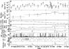 |
Fig. 1 Dust flux deduced from COSIMA collections (a) and b)) and spacecraft trajectory (c) to h)) plotted versus time from 11 August 2014 to 6 April 2015. a) Total dust flux per collection time period. b) Same as a) except for the time periods: dust flux is averaged on a monthly basis. c) Heliocentric distance (ref: JPL). d) Nucleo-centric distance (ref: ESA). e) Phase angle (ref: ESA). f) Off-nadir angle (ref: ESA). g) Latitude (ref: ESA). h) Spacecraft velocity with respect to the comet center (ref: ESA). |
The dust is not collected as a continuous flow in time, but shows a variability of several orders of magnitude on a very short time scale. For example, as shown in Fig. 1, between mid and late-January 2015, the dust flux could vary within four orders of magnitude from one day to the other. To compare the short-term variations of the dust flux with the spacecraft trajectory and pointings, the heliocentric and nucleo-centric distances, the phase angle (angle Sun-comet-Rosetta), the off-Nadir angle, the latitude, and the velocity of the spacecraft are plotted in the panels c to h of Fig. 1. No clear relationship can be seen between the dust flux short-term variability measured by COSIMA and a specific spacecraft flight configuration. The data analysis reveals instead that the short-term variability of the dust flux is mainly due to the collection of very large particles that fragment inside the instrument and which appear on the COSISCOPE images as clusters of particles. Evidence of fragmentation inside COSIMA of big parent particles into smaller daughter particles (we will call these events “fragmentation events” in the following) can be identified on the COSISCOPE images. An example is given in Fig. 2. The left image shows a target set with particles collected during one week in December 2014 (the particles are mainly located on the top target). The image in the middle shows the same target set after one additional week of exposure. Several new particles have been collected during the supplementary week, most of which are located on the mid-target on a 0.5 cm × 0.5 cm area around the upper-left screw. The distribution of these particles onto a small area indicates that they resulted from a large particle fragmentation that occurred upon impact or close enough to the target to maintain a small spatial dispersion, most likely on the wall of the dust funnel. Several of these fragmentation events have been identified by analyzing the spatial distribution of the particles on the target assembly. We assume that if the particles collected during one given exposure are not spatially randomly distributed, they result from the fragmentation of one large unique parent particle inside the funnel. In order to investigate whether the spatial distribution of the particles is random or not, we have divided the substrate into i sub-areas of equal size. Particles of each sub-area i were counted to obtain a particle number Ni. Here 27 areas were used, as illustrated in the right image of Fig. 2. In the case of random spatial distribution, the number of particles of each sub-area should follow the Poisson distribution:  (1)where
  is the mean value of the observed dataset N. Joint probability distribution of observing the dataset N is then
  (2)However, we consider here only the cases θ with the total particle number equal to the sum of observed particle numbers Ni. The probability of getting such an observation from the sum of Poisson distributed numbers is:
  (3)where S is the sum of observed numbers Ni. Applying Bayes’ theorem, we obtain:
  (4)This equation was verified by a Monte-Carlo simulation: when a random number generator adds +1 to the random cell iS times, we obtain a set of randomly distributed numbers Ni with the condition
  . Looping this process for one million times, we can estimate the frequency of the particular dataset N occurrence among all the possible value space θ. Results were in strict agreement with the analytically derived probability P(N | θ).
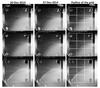 |
Fig. 2 COSISCOPE images of a dust particle fragmentation event. The images on the left show the three targets mounted on one target holder after one week of exposure (images 20-12-2014). The images in the middle show a cluster of particles that has been collected and settled around the screw on the upper left-hand corner of the mid-target after a further week of exposure (images 27-12-2014). Each target was imaged separately, the images are combined here respecting their configuration on the target holder. The images on the right show the grid used to analyze the spatial distribution of the particles (see text for detail). |
Integrating the probability P(N | θ) over θ is a difficult task, as the complexity of the problem grows with the size of the sample. Therefore we used a Monte-Carlo simulation to analyze the cumulative distribution function of P(N | θ) and derive the P-value of the observed dataset N.
Running the Monte-Carlo simulation as described above and calculating analytically the derived probability P(N′ | θ) for each iteration result N′, we can estimate the corresponding P-value from the frequency of occurrence of simulated datasets N′ with probability P(N′ | θ) equal or less than the probability of the observed data P(N | θ). A low P-value would then indicate an uneven distribution; for example, the spatial distribution of the collection shown in Fig. 2 has a P-value lower than 10-6.
In the following, for all collections for which the P-value is lower than 0.05, the particles are assumed to be the result of a fragmentation event within the instrument dust funnel and are considered as the daughters of a unique parent particle. One has to keep in mind that this method to identify fragmentation inside the funnel can introduce a bias toward both directions. The number of fragmentation events can be underestimated if the fragmentation occurs far from the target holder, for example directly at the entrance of the dust funnel or at a few meters from the spacecraft upon charging (Fulle et al. 2015), as this could result in a global random coverage of the target holder instead of a clustering. On the other hand, the number of fragmentation events can be overestimated if a more random distribution of single particles overlap with the fragments of a large particle broken inside the funnel, or if particles enter the dust funnel with a high angle (larger than 5°) as they would be confined within a small area on the target set and thus show clustering instead of a random spatial distribution. At small incident angles (between 2 and 5°), we estimate that about 60% of the particles do not collide at all with the funnel and are thus collected directly on the target assembly.
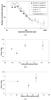 |
Fig. 3 a) Size distribution of the particles collected by COSIMA. In this representation, the bins have the same size on a logarithmic scale, and the power index derived from this curve is similar to the index of a cumulative size distribution. The fragmentation inside the instrument was taken into account by assuming that all particles from a fragmentation event are the daughters of a larger parent particle whose equivalent diameter is estimated by summing the volume of all the daughter particles. The different size distributions shown here by the black, white, and gray dots are obtained assuming fragmentation events if the P-values are lower than 0.05, 0.03 and 0.01 respectively. The dotted line represents the fitted power law for particles larger than 100 μm, the solid and dashed lines are the fitted power laws for the size distributions of the particles between 30 μm and 100 μm represented by the black dots and the gray dots respectively. The error bars are 1σ errors, for values lower than 100 counts. The error bars are derived from Gehrels (1986). b) Variation of the cumulative power index for particles with sizes between 30 μm and 100 μm and using a P-value lower than 0.05 for fragmentation events determination with respect to heliocentric distance, and c) to nucleo-centric distance. |
3.1. Size distribution of the dust particles
The sizes of the particles collected on the COSIMA targets range from one pixel (about 14 μm in diameter) to about 800 μm. There is no evidence for the presence of very small dust under the COSISCOPE resolution collected by COSIMA, that is, nanometer to micrometer-sized particles. No brightening of the target background that can be attributed to very small dust has been detected as the target material is much darker than the cometary particles. The target material has typically a brightness of a few Digital Numbers (on a range from 0 to 1023 DN), whereas the particles can reach 100 to 200 DN Langevin et al. (2016). If the brightness of the target material can slightly vary from one image to another due to its configuration with respect to the LEDs (the focus or the tilt can change between two images), the variation of the background does not exceed a few DNs when comparing the images taken before and after exposure to the cometary flux. On the other hand, no evidence for the presence of such nm-size dust particles in the time-of-flight secondary-ion mass spectra taken before and after target exposure to the cometary flux have been seen so far.
The cumulative size distribution of the particles detected by COSIMA is shown in Fig. 3a. As fragmentation inside the dust funnel is a major issue for determining the size distribution of the particles, we represented three different cases: the size distribution assuming that particles collected during one exposure are the result of a fragmentation event if the P-value derived by the method described above is lower than 0.05 or 5% level of confidence (black dots), if the P-value is lower than 0.03 or 3% level of confidence (white dots), and if the P-value is lower than 0.01 or 1% level of confidence (gray dots). The size distribution of the dust particles appears to follow three trends: the particles smaller than 30 μm show a flat distribution. Between 30 μm and 150 μm, the size distribution follows a power law of the form r− 1.9 ± 0.3. The value of the power index is close to the values obtained by Fulle et al. (2004, 2010), Kelley et al. (2009), Ishiguro (2008), from ground-based observations of 67P’s tail during its previous apparitions, which found indices for a cumulative size distribution of, respectively, −2.0 to −2.5, −2.5, −2.5, and −2. At larger sizes, the slope of the size distribution is close to −0.8, this value being consistent with the one of −1 derived by GIADA for compact particles (Rotundi et al. 2015). We neglect here dust ejection anisotropy and thus, give a size distribution of the dust particles at the spacecraft. It is not directly comparable to the size distribution measured at the surface of the nucleus. We will only discuss here the differences between the properties of the particles measured on the surface of the nucleus by other instruments with their properties when they have reached the spacecraft measured by COSIMA (see Sect. 4).
The power indices of the cumulative size distribution derived for single collections are plotted with respect to the heliocentric distance and to the distance to the nucleus in Figs. 3b and c respectively. There is no clear relation between the power index and these two parameters, implying that the increase in activity from 3.5 AU to 1.9 AU did not lead to a change in the size of the ejected particles that would be detectable at the spacecraft, and that the particles collected by COSIMA keep the same size distribution from at least 10 km to 30 km from the comet center.
3.2. Evolution of the flux of dust
The rate of dust collected by COSIMA shows large variations on a day to day timescale but if one looks at the dust flux averaged on a monthly basis shown in Fig. 1b, it is appears smoother. One can see that the dust flux is slowly increasing between August 2014 and February 2015 from a heliocentric distance of 3.4. AU to a distance of 2.3. AU. The dust flux observed by COSIMA decreased after February (below 2.4 AU) due to the aberration effects induced by the higher spacecraft velocity (>0.7m/s, in comparison to the usual velocity of 0.1–0.2 m/s). In mid-February and the end of March 2015, fast fly-bys were performed with closest approach distances from the comet center of about 10 km and 20 km, and a spacecraft velocity of 1.25 m/s and 1.14 m/s respectively. The dust velocity in the coma of 67P as measured in situ by GIADA was of the order of 0.1 to 10 m/s (Rotundi et al. 2015; Della Corte et al. 2015). Therefore, it is likely that, due to the aberration angle (the spacecraft was pointing toward the nucleus), dust could not be collected. The lack of collection of dust during the February fly-by in comparison to the March fly-by could be due to the different regions above which the spacecraft was flying that could have been more active in March.
From photometric ground-based observations at previous apparitions of the coma of 67P, it was determined that the dust flux evolved following a law of the form  , with α varying between 3 (Ishiguro 2008), 5.08 (Agarwal et al. 2007) and 5.8 (Kelley et al. 2009) according to different models used by these authors. We can compare the in situ dust flux derived by COSIMA to these models. The evolution of the dust flux with respect to the heliocentric distance has to be determined at a fixed distance from the nucleus to avoid bias due to its radial variations. Rosetta spent a few weeks in terminator orbit at a distance of about 28 km from the comet nucleus between mid-December 2014 and the end of January 2015. These data were therefore used, as well as data obtained in September 2014 at about 28 km nucleus distance with a phase angle of 80° and data obtained in March at 30 km with a phase angle of 70°. The variation of the dust flux with the heliocentric distance is given by the black dots in Fig. 4, the data are average in each bin of 0.1 AU and the error bars represent the standard deviation of the fluxes measured in each bin. A very rough estimate of the power index that best fits the COSIMA data would be around −4.2 ± 0.6. As the dust fluxes vary even at fairly constant distance to the nucleus and similar phase angles (80°–90°), it is unsatisfying to fit the COSIMA data directly to determine a power law for the dust flux evolution; we can only compare them with models. The closest to our value from the literature is the −5.08 value from Agarwal et al. (2007); for comparison, the above mentioned power laws are superimposed on the COSIMA data in Fig. 4.
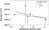 |
Fig. 4 Variation of the flux of dust collected between 25 and 30 km from the comet center with respect to the distance of the Sun. The data are averaged on distance bins of 0.1 AU, the vertical error bars give the standard deviation of the fluxes in each bin. The lines represent the models from the literature: black solid line: |


We normalized all dust fluxes to the solar distance using the power index of −5.08 and investigated how the dust flux evolves with distance to the nucleus center, the latitude, the spacecraft velocity, and the local time. We have separated the fluxes at low phase angle, that is, a phase angle smaller than 45° (Fig. 5), and the fluxes close to the terminator, that is, a phase angle between 75° and 90° (Fig. 6). In each figure, the left column shows the mass fluxes and the right column shows the particle fluxes. For the collection periods identified as fragmentation events, the number of particles collected is assumed to be only one, or in other words, all particles collected during a fragmentation event are assumed to be the daughters of a single parent particle. For the period with a very low number of particles collected (lower than 100), the error bars are derived from Gehrels (1986).
We superimpose in Figs. 6a and b the  law with a dashed line. If the global behavior of the dust flux roughly follows the law for the fluxes measured at high phase angle, the fluxes measured at low phase angle show more dispersion (Figs. 5a and 5b) and we cannot draw a power law that would describe the data. In the time-period reported here, that is, August 2014 to May 2015, the designed spacecraft pointings are mostly at high phase angle, thus the statistics are much better at high phase angle than at low phase angle.
If one compares the mass and particle fluxes at low and high phase angle, we can see that large parent particles leading to fragmentation events are mainly collected at low phase angle. If in both cases (high and low phase angle), about 40% (41% and 47% respectively) of the exposure periods lead to a fragmentation event, 99.8% of the particles collected at low phase angle are associated with fragmentation events whereas 81% of the particles collected at high phase angle are associated with fragmentation events. This implies that the parent particles collected at low phase angle are either larger than the ones collected at high phase angle, leading to a larger number of fragments, and/or that they are faster. This difference can be explained as large particles can be lifted more easily by gas drag around the sub-solar point since the illumination, and thus probably the coma gas density, is higher at this location.
The evolution of the dust flux with the latitude and the local time is not very obvious from COSIMA data, the variations of the flux being of several orders of magnitude at a given latitude. At far distances from the comet nucleus (30 km and beyond), the origin of the dust particles is not easy to trace back. Given the long exposure time of COSIMA collections, the uncertainty in the origin of the particles is very high and explains the large variations in the fluxes at a given latitude or local time.
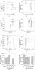 |
Fig. 5 Low phase angle (0°–45°) mass fluxes of dust (left column) and particle fluxes (right column) normalized to the solar distance at 3 AU and plotted against nucleo-centric distance a), b), latitude c), and d), spacecraft velocity e), f), and local time g), h). The error bars on the mass fluxes are given by using densities of 2500 kg/m3 and 100 kg/m3. The error bars on the particle fluxes represent the 1σ error. For collection periods with low number of particles (less than 100), the error bars are derived from Gehrels (1986). |
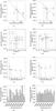 |
Fig. 6 High phase angle (75°–90°) mass fluxes of dust (left column) and particle fluxes (right column) normalized to the solar distance at 3 AU. a), b) Fluxes plotted versus the distance to the comet center. The data are averaged on nucleo-centric distance bins of 10 km. The dashed line represent the |
3.3. Dust flux of particles of different morphological types
The particles collected by COSIMA show a wide range of textures and shapes: compact particles, rubble piles, shattered clusters, and glued clusters (Langevin et al. 2016). Figure 8 shows a typical example for each morphological type. We can define two main populations: the compact particles, which correspond to particles that did not fragment or flatten on the COSIMA targets, and the porous aggregates which includes the rubble piles, the shattered clusters, and the glued clusters. To find clues to the physical structure of the comet nucleus, it is important to know whether these populations are intimately mixed or if they behave like distinct populations that come from distinct regions of the nucleus. We compared the evolution of the dust flux of the two different populations of particles to analyze their behavior in more detail. As particles smaller than 100 μm are difficult to classify, this analysis addresses particles larger than 100 μm only.
The flux of dust particles can also be plotted for each mass bin if one assumes a value for the density as shown in Fig. 7. In this figure, the black dots are the fluxes derived assuming a density of 1000 kg/m3 that can be compared to other instruments and/or missions around other comets. The open circles are obtained by using a size-dependant density as described in Hornung et al. (2016, in revision). The dust flux is normalized to 10 km distance of the nucleus and to 3 AU distance of the Sun assming a 1 /r2 law for the dust flux dependence on nucleus distance and a  variation (Agarwal et al. 2007).
The fluxes of compact particles and porous aggregates are depicted in Fig. 9 by the gray squares and black diamonds respectively. In this plot, the density is assumed to be 1000 kg/m3 in both cases; therefore, the plot is more representative of the evolution of the collected volume of each type of particle rather than of the mass. The large particles (i.e. larger than 100 μm) collected by COSIMA at heliocentric distances greater than 3.1 AU are only porous aggregates; the first large compact particles are collected at 3.1 AU. The ratio between the compact particles’ and the porous aggregates’ fluxes remains almost stable until January 2015, that is, between 3.1 AU to 2.6 AU from the Sun. Below 2.6 AU from the Sun, the COSIMA dust collection is dominated again by porous aggregates, in particular, by very large (larger than 500 μm) porous aggregates that fragmented inside the instrument. These large aggregates do not contain a significant fraction of large compact particles.
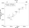 |
Fig. 7 Differential flux of dust collected in each mass bin normalized to the solar distance at 3 AU and to 10 km distance from the comet assuming |

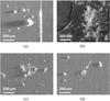 |
Fig. 8 COSISCOPE images of particles from the four morphological types defined in the text: a) compact particle, b) rubble pile, c) shattered cluster, d) glued cluster. |
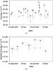 |
Fig. 9 Dust flux of porous aggregates (black diamonds) and compact particles (gray squares) larger than 100 μm a), as well as their monthly average b), from mid August 2014 to April 2015. |
The dust flux is dominated by the porous aggregates as they tend to be much larger (sizes up to almost a millimeter) compared to the compact particles (the biggest compact particle collected being about 250 microns in size). If we compare the number of particles of the two morphological types (Fig. 10), the compact particles represent about half of the collection. In September 2014, no compact particles were collected but we cannot exclude the possibility that this is due to the small statistics on large particles during that time.
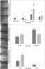 |
Fig. 10 Number of porous aggregates (dark gray) and compact particles (light gray) on each targt set. The number of porous aggregates is determined by assuming that all aggregates collected during a fragmentation event originate from a single aggregate. The compact particles on the other hand are counted as independent particles. The error bars are derived from Tables 1 and 2 of Gehrels (1986) and represent the upper and lower limit of the Poisson single sided distribution for a 1σ confidence level. The images on the left show the target holders after the end of the whole period in which they were exposed. |
4. Discussion
The dust particles collected by COSIMA are not collected as a continuous flow but appear bunched in time. It is important to note that 99% in number of the dust particles collected from mid-February 2015 to April 2015 appeared in “bursts” of large particles while less than 1% in number of particles of the COSIMA collection is composed of small dust (i.e. smaller than 100 μm) in this same time period. At the same time, COSIMA did not observe a background of steady dust flux. In particular, an improvement of the collection time-resolution after January from one week to one day allowed for the identification of the zero collection for periods of time extending up to a few days. Clusters of coma dust particles were observed in previous space missions to comets: in the coma of comet 1P/Halley (Simpson et al. 1987), 81P/Wild (Green et al. 2004), and 9P/Tempel (Economou et al. 2013). Large variations in the dust flux of 67P are reported by GIADA, which detected several “dust showers”, that is, from tens to hundreds of particles arriving in a few seconds (Fulle et al. 2015; Della Corte et al. 2015). It is important to note that the large collections detected by COSIMA and the GIADA dust showers are not correlated in time. As GIADA and COSIMA are located on the same side of the spacecraft, at a distance of about a meter, it is very unlikely that the sudden large fluxes of dust correspond to the crossing of a major structure such as a jet: they are more likely to be the result of the splitting of a few large particles very close to the instruments. In the case of COSIMA, disintegration likely occurs by impact on the walls of the dust funnel. Furthermore, disruption due to electrical charging might occur when the particles approach the spacecraft (Fulle et al. 2015). The observation of “bursts” of particles raises a major issue if one wants to analyze the behavior of the dust in cometary comae, in particular for COSIMA which has a time-resolution of at least a day. The general evolution of the particle fluxes can only be described after being averaged over long periods of time.
From the flux of dust collected by COSIMA from 10 km up to 250 km from the nucleus, there is a trend toward a law for particles collected when the spacecraft was pointing at high phase angle implying that the particles collected in this configuration do not show a fragmentation pattern along their way out from the nucleus. At low phase angle, the fluxes are more dispersed. One way to address this issue is to look at the size distribution of these collected particles. If they fragment, we should be able to detect a transfer of mass from large particles into smaller ones. We can thus compare the data obtained at the spacecraft with the measurements of the size distribution obtained at the surface of the comet by the ROLIS instrument on board of Philae lander. The size distribution at the first touchdown at the comet measured by ROLIS (Mottola et al. 2015) follows a law with a cumulative power index of −2.2 ± 0.1 in the rough areas and −2.8 ± 0.2 in the smooth areas, for particles larger than 1 cm in size. The size distribution of particles with sizes ranging from 1 mm to 1 cm ejected from the nucleus is deduced by OSIRIS, which obtains a cumulative power index of −3 (Rotundi et al. 2015), close to the ROLIS values for the smooth terrains. At sizes smaller than a millimeter, GIADA obtains a shallower size distribution with a cumulative power index of −1 (Rotundi et al. 2015). The size distribution measured by COSIMA at the spacecraft for particles from 150 μm to almost a millimeter follows a similar behavior as the GIADA distribution since the power index is −0.8 ± 0.1. This knee in the size distribution can be explained in two ways: either the size distribution at the surface of the comet changes for particles smaller than a millimeter and if particles are ejected with the same efficiency by gas drag no matter their size, or the knee can be a consequence of the threshold of the size of liftable particles by gas drag as described by Gundlach et al. (2015). Fulle et al. (2016) propose that the knee is created during the fallback of the dust particles. The particles under 1 mm are more efficiently repulsed by the low gas drag on the night side of the nucleus than the larger ones.
For smaller sizes, down to 30 μm, the cumulative size distribution measured at the spacecraft by COSIMA is slightly steeper, with a power index of −1.9 ± 0.3, very similar to the size distribution of the very large (>1 mm) particles on the surface of the nucleus on the rough terrains. If these small particles collected by COSIMA were produced by fragmentation of the larger ones along their way from the comet to the spacecraft, one would expect that their velocity would be similar to the velocity of the large particles, or at least, small particles would show more variation in their velocity distribution since the collection should gather fast, small dust particles lifted from the comet and the particles produced from the disruption of larger ones. COSIMA does not measure the velocity of the particles directly but a lower limit on the velocity of the collected particles can be estimated from the aberration due to the spacecraft velocity when pointing towards the nucleus. We can use this phenomenon to check if a filtering of particles according to their size occurs and thus, deduce a velocity dependence with the size of the particles. Figure 11a shows the typical sizes of the collected particles with respect to the spacecraft velocity. The particles arriving with a very high angle, that is, the particles fragmented on the wall of the funnel, are not represented. The particles shown are thus the ones which are not associated with a fragmentation event. We assume that they have been able to make their way to the COSIMA target without fragmenting in the funnel. One can see a strong cut-off on the larger size that COSIMA detects, more large particles being collected at low spacecraft velocity. This implies that the larger particles are slower than the small ones. This behavior still holds when adding particles fragmented in the funnel (the parent particles of the fragmentation events). The cut-off velocity dependence according to the size of the particle that we can deduce from COSIMA data follows a power law of index −0.8 ± 0.3. If we also include the particles that collided with the dust funnel, then the power index reaches −0.5 ± 0.1 which is close to the ejection velocity dependence on the size stated by Agarwal et al. (2007), shown by the dashed line in Fig. 11a.
The ratio between large and small particles is shown in Fig. 11b by gray and white dots. One can see that the large particles are filtered at large spacecraft velocities. Above 0.5 m/s, no particle larger than 50 μm is collected (represented by the arrows in Fig. 11b), indicating that most of these particles were slower than 3 m/s at the time of the collections. If we focus on the small particles (smaller than 50 μm), no filtering can be observed; the ratio of particles in the range 30–50 μm compared to the number of particles in the range 10 to 30 μm (black squares in Fig. 11b) is very stable at spacecraft velocities from 0.15 to 1.1 m/s. We can deduce from this analysis that the small particles are faster than the large ones, and are not produced by fragmentation of large particles along their way to the spacecraft but are released directly at the comet surface, at the footprint of the acceleration region. The models of dust ejection by gas drag (Blum et al. 2015; Gundlach et al. 2015) show that aggregates smaller than a certain threshold (a centimeter in these models) are not easily ejected from the surface of a cometary nucleus as the binding forces between these aggregates are too high. To explain the presence of small dust, we propose the following scenario: when a cm- or mm-sized particle is lifted off the nucleus surface by gas drag, it breaks out from its neighboring particles. Both large and small particles are released in the breaking process and are then accelerated by the gas drag according to their size and density.
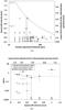 |
Fig. 11 a) Scatter plot showing the typical size of the collected particles collected at different spacecraft velocities. The arrows represent the collection periods for which no particles have been detected and thus correspond to an upper limit of the size of eventually collected particles (the limit being given by the resolution of the COSISCOPE). In this plot, the particles fragmented on the walls of the funnel are not included. The dashed line represent the v ~ size-0.5 dependence. b) Gray dots: ratio of the number of particles larger than 100 μm/number of particles smaller than 100 μm. White dots: ratio of the number of particles larger than 50 μm/number of particles smaller than 50 μm. The arrows represent null ratios obtained in these two cases for spacecraft velocities larger than 0.5 m/s for which no particles above 50 μm have been collected. Black squares: ratio of the number of particles with sizes comprised between 30 μm and 50 μm/number of particles between 10 μm and 30 μm. In all cases, the error bars represent a 1σ error. |
The dust flux dependence on particle size is rather flat below 30 μm (Figs. 3a and 7). One has to be careful with the interpretation of the data since this size (1–2 COSISCOPE pixels) approaches the detection limit of COSIMA. This turn-off point is an important parameter to determine as it illustrates the typical size to which an aggregate can be separated into its smaller sub-constituents. As the aggregate gets smaller, the tensile strength increases and it becomes more difficult to overcome the binding forces holding together these constituents, indicating that a stronger force than Van der Waals is needed to separate the sub-constituents from each other. The turn around point at about 30 μm is also observed with the COSISCOPE in the size distribution of individual particles that fragment upon impact at low velocity on the COSIMA targets (Hornung et al. 2016, in revision).
When comparing to comet samples brought back by the Stardust mission, the two morphological families of particles (compact and porous aggregates) collected by COSIMA might be linked to the different types of tracks observed in the Stardust aerogel that collected dust particles in the coma of 81P/Wild (Joswiak et al. 2012). The compact particles could be similar to the refractory particles that produced the carrot-shaped tracks observed on the Stardust aerogel collector; the COSIMA porous aggregate particles could be related to the loosely bonded particles that produced the bulbous-shape tracks observed in the Stardust aerogel collector. The compact particles might be refractory material, likely formed in hotter parts of the protoplanetary disk, incorporated into the comet nucleus during its formation and mixed with a more abundant porous material similar to chondritic-porous Interplanteary Dust Particles that are thought to originate from comets (Brownlee et al. 1995; Bradley 2003). The relative number of the compact and porous aggregate particles in the COSIMA collection varies with time. Porous aggregates dominate the COSIMA collection from mid-August 2014 to October 2014. Compact particles appeared for the first time by the end of September 2014. From October 2014 (3.4 AU from the Sun) to mid of January 2015 (2.5 AU), the variation of the ratio in volume of porous aggregate to compact particles stays almost constant (approx. one to four) and then increases by about a factor of ten. In number of particles, the porous aggregates are less abundant than compact particles in the later phase, however, these aggregates are much larger than the ones collected up to December, beyond 2.8 AU from the Sun.
If we compare the COSIMA data with the GIADA data, Della Corte et al. (2015) also report a number of detections of aggregates higher than compact particles. Like COSIMA, GIADA also collects showers of particles. Once these showers are put back together, the number of compact particles dominates the GIADA collection by a factor comprised between 2.6 and 14, which is a factor of two to seven higher than the COSIMA observations. The classes defined as compact and porous aggregates can be slightly different for the two instruments and one cannot exclude that the COSIMA compact or aggregates are different from the GIADA compact and fluffy classifications, since both instruments measure different physical parameters (Kissel et al. 2007; Colangeli et al. 2007). On one hand, the COSIMA particles are classified from the morphology derived from optical images. Two biases can be introduced: first, if very slow aggregates are collected without fragmenting on the target, they would show a morphology close to the compact particles and could be mis-classified. Second, if a slow compact particle impacts the target and does not stick to it, then it will not be detected. GIADA, on the other hand, classifies particles based on the type of signal detected. This classification can also introduce a bias since one cannot completely exclude the possibility that less porous aggregates could also be detected by the impact sensor and thus be mis-classified.
The COSIMA data are clearly dominated in volume by porous material. The compact particles seem to appear as individual particles with sizes not larger than a few hundreds of microns. All large clusters have been carefully checked to search for mixed particles, that is, cluster-type particles with compact components. No mixed particle was found so far in the COSIMA collection (see also the discussion in Langevin et al. 2016). The same observation can be made with larger aggregates. The compact particles collected during fragmentation events are not located on the same target as the majority of the porous dust particles, as can be seen in the images shown in Fig. 10. In the target set shown on the top of the figure, most of the compact particles are located on the bottom target of the holder, whereas aggregates are spread on all three targets. Similarly, the target set shown on the bottom of the figure contains a lot of aggregate material on the top-target of the holder, while the compact particles are located on the bottom-target. If the compact particles were embedded inside the aggregates, one could expect the compact particles to be located close to the impact point, or at least on the same target, or be surrounded by porous material. Here, the compact particles can be as far as two centimeters from the impact point on the target. This indicates that the compact component may have been already separated from the porous material before entering into the instrument. This implies that the large compact particles could be separated from each other in the comet by distances up to, at least, a millimeter, since millimeter-sized aggregates with no large compact particle inclusions are collected by COSIMA.
5. Conclusion
The COSIMA instrument on board Rosetta has provided data on the dust environment in the coma of 67P along its pre-perihelion orbit between 3.5 AU to 1.9 AU. The study of the dust properties with sizes ranging from 14 μm to about 800 μm was possible as the instrument can collect dust at very low speed, preventing particles from being completely destroyed upon impact. The absence of carters on the targets and the collection of large fragments of particles is in agreement with velocities of cm/s to a few m/s, the large particles being slower than small particles.
We have analyzed the flux of dust particles around the nucleus at various nucleo-centric distances. In situ collected dust does not arrive in a continuous flow but in bursts, at all distances from the nucleus covered by the spacecraft in the time period reported in this paper, that is, from 8 km to 386 km. The dependence of the collection rate with the distance from the nucleus is different at low and high phase angles. Only the flux of particles collected at low phase angle shows a behavior different from the classical law. There is no evidence of fragmentation of large dust particles along their trajectory from the acceleration region to the spacecraft. The larger particles are cut-off at higher spacecraft veloctiy and therefore are slower than the smaller ones. For fragmented particles, one would expect a similar group velocity independent of particle size.
Large particles, with sizes close to a millimeter, are mainly collected at low phase angle and at about 30° to 50° of latitude, where the illumination of the Sun is high, and thus the gas density is higher. This size is still smaller than the threshold of liftable particles (Gundlach et al. 2015). The small dust particles, that is, smaller than 50 μm, are not produced by fragmentation of larger particles on their way from the nucleus to the spacecraft beyond the acceleration region, but are potentially released from the comet surface during the lift-off of larger particles and accelerated by the gas drag.
The collection rates of the two morphological types of particles observed, compact particles and porous aggregates, do not follow the same trend: the ratio between these two populations varies with time. The particles larger than 100 μm in size collected by COSIMA beyond 3.1 AU are porous aggregates, whereas compact particles appear later on. The ratio in volume of compact to porous aggregates measured during a stable period over three months is 25%, implying that the dust of 67P is mainly composed of porous material, very similar to the porous Interplanetary Dust Particles believed to originate from comets, and also contains compact particles with sizes up to a few hundreds of microns that could be represented in dust collected on Earth as compact chondritic particles.
Acknowledgments
COSIMA was built by a consortium led by the Max-Planck-Institut für Extraterrestrische Physik, Garching, Germany in collaboration with Laboratoire de Physique et Chimie de l’Environnement et de l’Espace, Orléans, France, Institut d’Astrophysique Spatiale, CNRS/Université Paris Sud, Orsay, France, Finnish Meteorological Institute, Helsinki, Finland, Universität Wuppertal, Wuppertal, Germany, von Hoerner und Sulger GmbH, Schwetzingen, Germany, Universität der Bundeswehr, Neubiberg, Germany, Institut für Physik, Forschungszentrum Seibersdorf, Seibersdorf, Austria, Space Research Institute, Austrian Academy of Sciences, Graz, Austria and is led by the Max-Planck-Institut für Sonnensystemforschung, Göttingen, Germany. The support of the national funding agencies of Germany (DLR, grant 50 QP 1302), France (CNES), Austria, Finland, and the ESA Technical Directorate is gratefully acknowledged. V. Della Corte, M. Fulle, and A. Rotundi were supported by the Italian Space Agency (ASI) within the ASI-INAF agreements I/032/05/0 and I/024/12/0. We thank the Rosetta Science Ground Segment at ESAC, the Rosetta Mission Operations Centre at ESOC and the Rosetta Project at ESTEC for their outstanding work enabling the Science return of the Rosetta Mission. Rosetta is an ESA mission with contributions from its member states and NASA. Rosetta’s Philae lander is provided by a consortium led by DLR, MPS, CNES and ASI.
References
- Agarwal, J., Müller, M., & Grün, E. 2007, Space Sci. Rev., 128, 79 [NASA ADS] [CrossRef] [Google Scholar]
- Agarwal, J., Müller, M., Reach, W. T., et al. 2010, Icarus, 207, 992 [NASA ADS] [CrossRef] [Google Scholar]
- Blum, J., Gundlach, B., Mühle, S., & Trigo-Rodriguez, J. M. 2015, Icarus, 248, 135 [NASA ADS] [CrossRef] [Google Scholar]
- Bradley, J. P. 2003, Treatise on Geochemistry, 1, 689 [NASA ADS] [Google Scholar]
- Brownlee, D. E., Joswiak, D. J., Schlutter, D. J., et al. 1995, in Lunar and Planetary Science Conference, 26, 183 [Google Scholar]
- Clark, B. C., Green, S. F., Economou, T. E., et al. 2004, J. Geophys. Res., 109, 12 [Google Scholar]
- Colangeli, L., Lopez Moreno, J. J., Palumbo, P., et al. 2007, Adv. Space Res., 39, 446 [NASA ADS] [CrossRef] [Google Scholar]
- Della Corte, V., Rotundi, A., Accolla, M., et al. 2014, J. Astron. Instrument., 3, 50011 [Google Scholar]
- Della Corte, V., Rotundi, A., Fulle, M., et al. 2015, A&A, 583, A13 [NASA ADS] [CrossRef] [EDP Sciences] [Google Scholar]
- Economou, T. E., Green, S. F., Brownlee, D. E., & Clark, B. C. 2013, Icarus, 222, 526 [Google Scholar]
- Fulle, M., Barbieri, C., Cremonese, G., et al. 2004, A&A, 422, 357 [NASA ADS] [CrossRef] [EDP Sciences] [Google Scholar]
- Fulle, M., Colangeli, L., Agarwal, J., et al. 2010, A&A, 522, A63 [NASA ADS] [CrossRef] [EDP Sciences] [Google Scholar]
- Fulle, M., Della Corte, V., Rotundi, A., et al. 2015, ApJ, 802, L12 [NASA ADS] [CrossRef] [Google Scholar]
- Fulle, M., Marzari, F., Della Corte, V., et al. 2016, ApJ, 821, 19 [NASA ADS] [CrossRef] [Google Scholar]
- Gehrels, N. 1986, ApJ, 303, 336 [NASA ADS] [CrossRef] [Google Scholar]
- Green, S. F., McDonnell, J. A. M., McBride, N., et al. 2004, J. Geophy. Res., 109, 12 [Google Scholar]
- Guilbert-Lepoutre, A., Schulz, R., Rożek, A., et al. 2014, A&A, 567, L2 [NASA ADS] [CrossRef] [EDP Sciences] [Google Scholar]
- Gundlach, B., Blum, J., Keller, H. U., & Skorov, Y. V. 2015, A&A, 583, A12 [NASA ADS] [CrossRef] [EDP Sciences] [Google Scholar]
- Hilchenbach, M., Kissel, J., Langevin, Y., et al. 2016, ApJ, 816, L32 [NASA ADS] [CrossRef] [Google Scholar]
- Hornung, K., Kissel, J., Fischer, H., et al. 2014, Planet. Space Sci., 103, 309 [NASA ADS] [CrossRef] [Google Scholar]
- Hornung, K., Merouane, S., Hilchenbach, M., et al. 2016, Planet. Space Sci., in press, DOI: 10.1016/j.pss.2016.07.003 [Google Scholar]
- Ishiguro, M. 2008, Icarus, 193, 96 [NASA ADS] [CrossRef] [Google Scholar]
- Joswiak, D. J., Brownlee, D. E., Matrajt, G., et al. 2012, Met. Planet. Sci., 47, 471 [Google Scholar]
- Kelley, M. S., Wooden, D. H., Tubiana, C., et al. 2009, AJ, 137, 4633 [NASA ADS] [CrossRef] [Google Scholar]
- Kissel, J., Altwegg, K., Clark, B. C., et al. 2007, Space Sci. Rev., 128, 823 [NASA ADS] [CrossRef] [Google Scholar]
- Langevin, Y., Hilchenbach, M., Ligier, N., et al. 2016, Icarus, 271, 76 [NASA ADS] [CrossRef] [Google Scholar]
- McDonnell, J. A. M., Evans, G. C., Evans, S. T., et al. 1987, A&A, 187, 719 [NASA ADS] [Google Scholar]
- Mottola, S., Jaumann, R., Schröder, S., et al. 2015, in Lunar and Planetary Inst. Technical Report, 46, 2308 [Google Scholar]
- Rotundi, A., Sierks, H., Della Corte, V., et al. 2015, Science, 347, 3905 [Google Scholar]
- Schulz, R., Stüwe, J. A., & Boehnhardt, H. 2004, A&A, 422, L19 [NASA ADS] [CrossRef] [EDP Sciences] [Google Scholar]
- Schulz, R., Hilchenbach, M., Langevin, Y., et al. 2015, Nature, 518, 216 [NASA ADS] [CrossRef] [Google Scholar]
- Simpson, J. A., Rabinowitz, D., Tuzzolino, A. J., Ksanfomaliti, L. V., & Sagdeev, R. Z. 1987, A&A, 187, 742 [NASA ADS] [Google Scholar]
- Snodgrass, C., Tubiana, C., Bramich, D. M., et al. 2013, A&A, 557, A33 [NASA ADS] [CrossRef] [EDP Sciences] [Google Scholar]
- Tozzi, G. P., Patriarchi, P., Boehnhardt, H., et al. 2011, A&A, 531, A54 [NASA ADS] [CrossRef] [EDP Sciences] [Google Scholar]
All Figures
|
Fig. 1 Dust flux deduced from COSIMA collections (a) and b)) and spacecraft trajectory (c) to h)) plotted versus time from 11 August 2014 to 6 April 2015. a) Total dust flux per collection time period. b) Same as a) except for the time periods: dust flux is averaged on a monthly basis. c) Heliocentric distance (ref: JPL). d) Nucleo-centric distance (ref: ESA). e) Phase angle (ref: ESA). f) Off-nadir angle (ref: ESA). g) Latitude (ref: ESA). h) Spacecraft velocity with respect to the comet center (ref: ESA). |
| In the text | |
|
Fig. 2 COSISCOPE images of a dust particle fragmentation event. The images on the left show the three targets mounted on one target holder after one week of exposure (images 20-12-2014). The images in the middle show a cluster of particles that has been collected and settled around the screw on the upper left-hand corner of the mid-target after a further week of exposure (images 27-12-2014). Each target was imaged separately, the images are combined here respecting their configuration on the target holder. The images on the right show the grid used to analyze the spatial distribution of the particles (see text for detail). |
| In the text | |
|
Fig. 3 a) Size distribution of the particles collected by COSIMA. In this representation, the bins have the same size on a logarithmic scale, and the power index derived from this curve is similar to the index of a cumulative size distribution. The fragmentation inside the instrument was taken into account by assuming that all particles from a fragmentation event are the daughters of a larger parent particle whose equivalent diameter is estimated by summing the volume of all the daughter particles. The different size distributions shown here by the black, white, and gray dots are obtained assuming fragmentation events if the P-values are lower than 0.05, 0.03 and 0.01 respectively. The dotted line represents the fitted power law for particles larger than 100 μm, the solid and dashed lines are the fitted power laws for the size distributions of the particles between 30 μm and 100 μm represented by the black dots and the gray dots respectively. The error bars are 1σ errors, for values lower than 100 counts. The error bars are derived from Gehrels (1986). b) Variation of the cumulative power index for particles with sizes between 30 μm and 100 μm and using a P-value lower than 0.05 for fragmentation events determination with respect to heliocentric distance, and c) to nucleo-centric distance. |
| In the text | |
|
Fig. 4 Variation of the flux of dust collected between 25 and 30 km from the comet center with respect to the distance of the Sun. The data are averaged on distance bins of 0.1 AU, the vertical error bars give the standard deviation of the fluxes in each bin. The lines represent the models from the literature: black solid line: |
| In the text | |
|
Fig. 5 Low phase angle (0°–45°) mass fluxes of dust (left column) and particle fluxes (right column) normalized to the solar distance at 3 AU and plotted against nucleo-centric distance a), b), latitude c), and d), spacecraft velocity e), f), and local time g), h). The error bars on the mass fluxes are given by using densities of 2500 kg/m3 and 100 kg/m3. The error bars on the particle fluxes represent the 1σ error. For collection periods with low number of particles (less than 100), the error bars are derived from Gehrels (1986). |
| In the text | |
|
Fig. 6 High phase angle (75°–90°) mass fluxes of dust (left column) and particle fluxes (right column) normalized to the solar distance at 3 AU. a), b) Fluxes plotted versus the distance to the comet center. The data are averaged on nucleo-centric distance bins of 10 km. The dashed line represent the |
| In the text | |
|
Fig. 7 Differential flux of dust collected in each mass bin normalized to the solar distance at 3 AU and to 10 km distance from the comet assuming |
| In the text | |
|
Fig. 8 COSISCOPE images of particles from the four morphological types defined in the text: a) compact particle, b) rubble pile, c) shattered cluster, d) glued cluster. |
| In the text | |
|
Fig. 9 Dust flux of porous aggregates (black diamonds) and compact particles (gray squares) larger than 100 μm a), as well as their monthly average b), from mid August 2014 to April 2015. |
| In the text | |
|
Fig. 10 Number of porous aggregates (dark gray) and compact particles (light gray) on each targt set. The number of porous aggregates is determined by assuming that all aggregates collected during a fragmentation event originate from a single aggregate. The compact particles on the other hand are counted as independent particles. The error bars are derived from Tables 1 and 2 of Gehrels (1986) and represent the upper and lower limit of the Poisson single sided distribution for a 1σ confidence level. The images on the left show the target holders after the end of the whole period in which they were exposed. |
| In the text | |
|
Fig. 11 a) Scatter plot showing the typical size of the collected particles collected at different spacecraft velocities. The arrows represent the collection periods for which no particles have been detected and thus correspond to an upper limit of the size of eventually collected particles (the limit being given by the resolution of the COSISCOPE). In this plot, the particles fragmented on the walls of the funnel are not included. The dashed line represent the v ~ size-0.5 dependence. b) Gray dots: ratio of the number of particles larger than 100 μm/number of particles smaller than 100 μm. White dots: ratio of the number of particles larger than 50 μm/number of particles smaller than 50 μm. The arrows represent null ratios obtained in these two cases for spacecraft velocities larger than 0.5 m/s for which no particles above 50 μm have been collected. Black squares: ratio of the number of particles with sizes comprised between 30 μm and 50 μm/number of particles between 10 μm and 30 μm. In all cases, the error bars represent a 1σ error. |
| In the text | |
Current usage metrics show cumulative count of Article Views (full-text article views including HTML views, PDF and ePub downloads, according to the available data) and Abstracts Views on Vision4Press platform.
Data correspond to usage on the plateform after 2015. The current usage metrics is available 48-96 hours after online publication and is updated daily on week days.
Initial download of the metrics may take a while.