| Issue |
A&A
Volume 595, November 2016
|
|
|---|---|---|
| Article Number | A26 | |
| Number of page(s) | 13 | |
| Section | Planets and planetary systems | |
| DOI | https://doi.org/10.1051/0004-6361/201629088 | |
| Published online | 24 October 2016 | |
Radial velocity observations of the 2015 Mar. 20 eclipse
A benchmark Rossiter-McLaughlin curve with zero free parameters
1 Georg-August Universität Göttingen,
Institut für Astrophysik, Friedrich-Hund-Platz 1, 37077 Göttingen, Germany
e-mail: This email address is being protected from spambots. You need JavaScript enabled to view it.
2 Max-Planck Institut für
Sonnensystemforschung, Justus-von-Liebig-Weg 3, 37077
Göttingen,
Germany
Received:
10
June
2016
Accepted:
31
August
2016
Abstract
Spectroscopic observations of a solar eclipse can provide unique information for solar and exoplanet research; the huge amplitude of the Rossiter-McLaughlin (RM) effect during solar eclipse and the high precision of solar radial velocities (RVs) allow detailed comparison between observations and RV models, and they provide information about the solar surface and about spectral line formation that are otherwise difficult to obtain. On March 20, 2015, we obtained 159 spectra of the Sun as a star with the solar telescope and the Fourier Transform Spectrograph at the Institut für Astrophysik Göttingen, 76 spectra were taken during partial solar eclipse. We obtained RVs using I2 as wavelength reference and determined the RM curve with a peak-to-peak amplitude of almost 1.4 km s-1 at typical RV precision better than 1 m s-1. We modeled the disk-integrated solar RVs using well-determined parameterizations of solar surface velocities, limb darkening, and information about convective blueshift from 3D magnetohydrodynamic simulations. We confirm that convective blueshift is crucial to understand solar RVs during eclipse. Our best model reproduced the observations to within a relative precision of 10% with residuals lower than 30 m s-1. We cross-checked parameterizations of velocity fields using a Dopplergram from the Solar Dynamics Observatory and conclude that disk-integration of the Dopplergram does not provide correct information about convective blueshift necessary for m s-1 RV work. As main limitation for modeling RVs during eclipses, we identified limited knowledge about convective blueshift and line shape as functions of solar limb angle. We suspect that our model line profiles are too shallow at limb angles larger than μ = 0.6, resulting in incorrect weighting of the velocities across the solar disk. Alternative explanations cannot be excluded, such as suppression of convection in magnetic areas and undiscovered systematics during eclipse observations. To make progress, accurate observations of solar line profiles across the solar disk are suggested. We publish our RVs taken during solar eclipse as a benchmark curve for codes calculating the RM effect and for models of solar surface velocities and line profiles.
Key words: line: formation / line: profiles / methods: observational / techniques: radial velocities / techniques: spectroscopic / Sun: rotation
© ESO 2016
1. Introduction
The observation of radial velocities (RVs) of the Sun as a star is gaining interest in both solar and exoplanet communities. For solar applications, the availability of methods for computing one single parameter (the RV) from sometimes complex solar data and its comparison to other proxies opens new possibilities to search for physical relations. For the exoplanet community, the Sun is the one benchmark object on which methods can be tested with precision observations that offer more information than is available for any other star, such as limb darkening and surface velocity fields.
Obtaining RVs in stars involves measuring the Doppler shift of spectral lines at different times of observation. There are several ways to precisely determine a shift of spectral lines. They all have in common that a change in the line profile shape caused by an emerging active region on the star, for instance, can mimic a Doppler shift of several m s-1 (see, e.g., Fischer et al. 2016, and references therein). Finding ways to account for this type of bias is currently an important step in the search for Earth-like extrasolar planets (e.g., Hatzes 2013; Robertson et al. 2014, 2015; Anglada-Escudé et al. 2016). In the context of stars, it has been realized that m s-1 precision can only be reached when stellar surface velocities, and in particular the effect of magnetic activity on convective blueshift, are thoroughly understood (Lagrange et al. 2010; Meunier et al. 2010a,b; Dumusque et al. 2014; Marchwinski et al. 2015; Haywood et al. 2016).
The Sun provides an invaluable reference for understanding the influence of stellar surface velocity fields and active regions because it is possible to relate precision RV observations to spatially resolved solar surface information (Meunier et al. 2010b; Haywood et al. 2016). However, it is extremely difficult to obtain solar disk observations with m s-1 precision or better, and current solar Dopplergrams are known to exhibit severe problems in this respect (Couvidat et al. 2012b; Welsch et al. 2013). Furthermore, measuring precise Sun-as-a-star RVs is very challenging because the spatial extension of the Sun implies that feeding light from the Sun into a spectrograph involves the problem of collecting light from all areas of the solar disk equally. Earlier attempts have demonstrated this difficulty (Jimenez et al. 1986; Deming et al. 1987; Deming & Plymate 1994; McMillan et al. 1993) but there is new motivation for instruments facing this challenge, for example, observing the Sun with HARPS (Dumusque et al. 2015) and in the Göttingen Solar Radial Velocity Project used for this work (Lemke & Reiners 2016).
A particularly fruitful exercise to understand the effects across an extended stellar disk in RV measurements is the observation of an eclipse of the Sun by one of its planets or the Moon. During eclipse, solar and stellar RVs exhibit the so-called Rossiter-McLaughlin (RM) effect (Rossiter 1924; McLaughlin 1924) with excursion of the RV curve to the blue and the red in proportion to the rotational velocity of the star and to the amount of the surface eclipsed (e.g., Ohta et al. 2005; Gaudi & Winn 2007; Torres et al. 2008; Fabrycky & Winn 2009). Observations of planetary transits of the Sun can also be performed with night-time telescopes observing the light reflected from other bodies of the solar system in order to avoid the effect of the spatially extended solar disk (e.g., Molaro et al. 2013, 2015). The RM effect in stars is used to determine the geometry of planetary systems. Convective blueshift influences the shape of the RM curve and potentially biases measurements of planetary system geometries (Shporer & Brown 2011; Boué et al. 2013; Cegla et al. 2016b,a). A planetary transit can also be used to observe local stellar line profiles (Dravins et al. 2015), and in the same sense, observations of the eclipsed Sun provide a unique opportunity to gather information about local solar line profiles and about the influence of convective blueshift on RM measurements.
Takeda et al. (2015) carried out observations of the solar eclipse visible in Japan on May 21, 2012, with the aim to extract information on solar rotation. At maximum, the Moon eclipsed 93% of the visible Sun during their observations. They showed an RM curve with a peak-to-peak amplitude of almost 2 km s-1 and calculated a model of the RV curve that matches within a standard deviation of 41 m s-1. Their model includes solar differential rotation and limb darkening, and they attempted to gain information on solar surface rotation from their RV curve. Takeda et al. (2015) also provided information about the spectral line shape during eclipse and discussed deviations between ATLAS9 solar model calculations (Kurucz 1993) and their observations.
In this work, we investigate our solar eclipse observations from Mar 15, 2015, with a maximum eclipse of 75.9%. We argue that solar surface rotation and large-scale granulation patterns are relatively well described from different tracers (Snodgrass 1992; Del Moro 2004). On the other hand, the effect of convective blueshift is less well quantitatively understood, in particular its variation across the solar disk (e.g., Beckers & Nelson 1978). In addition, convective flows can be suppressed in the presence of magnetic fields (Livingston 1982), with the consequence that magnetic areas affect RV observations of active stars and the Sun. Therefore, we assume in our work that the geometry of the eclipse as well as surface rotation and granulation velocity fields are correctly known from independent information. As the most critical parameters for modeling solar RVs we identify line intensity changes across the solar disk and the dependence of convective blueshift on solar limb angle.
2. Instrument
The Institut für Astrophysik, Göttingen (IAG) operates a Fourier transform spectrograph (FTS) Bruker IFS 125 HR. Details of the instrument and observing modes are described in Reiners et al. (2016) and Lemke & Reiners (2016). We observed the Sun as a star by feeding light of a 52′ field of view from the flat mirrors of a siderostat into a 800 μm fiber that transports the light into our optics laboratory. We sent the light through an absorption cell filled with I2 and into our FTS. Lemke & Reiners (2016) showed that the photon noise limit in our radial velocity (RV) observations is below 10 cm s-1 but stellar and instrumental noise limit our RV precision; we found RV drifts on the order of 10 m s-1 h-1 in other measuring campaigns. Based on this experience, we cannot exclude drifts of this amplitude for the observations used in this work. These drifts, however, were typically rather linear for many exposures. In addition, the RV curves sometimes showed sudden jumps of a few m s-1, but they could be easily identified. They were probably caused by manual readjustment of the siderostat tracking mechanism.
A second problem we only realized after observations is improper logging of the start time of exposure. The FTS control software logged the time of observation as given by the control computer. This machine unfortunately was not properly synchronized to a time standard, with the consequence that the absolute time of observation is unknown with an uncertainty of several ten seconds, which is the typical time we found the clock to be off.
3. Observations
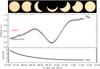 |
Fig. 1 Upper panel: photographs of the solar eclipse taken at our observatory; middle panel: observed flux normalized to 1.0 at 11:00 UT, black open circles show flux integrated from our observed spectra, the red line shows the flux from our extinction model and eclipse (see text); bottom panel: airmass during our observations. Times are given in UT. |
The solar eclipse occurred in Göttingen in the morning hours of March 20, 2015, with its maximum at 09:42 UT (10:42 local time). We obtained 159 observations of the Sun as a star between 07:05 and 12:05 UT. Details of observations are provided in Table A.1. The interferograms were sampled in fully symmetric forward-backward mode, each scan took 97 s. The resolution, R, of the transformed spectra is several 105. The first spectrum was taken at airmass 3.8. At the start of the eclipse (08:35 UT), the Sun was at airmass 2.2. After the eclipse the Sun culminated at airmass 1.6. Our spectra are sampled with constant step size of 0.01 cm-1, that is, Δλ = 0.0055 Å at 6000 Å. We measured the signal-to-noise ratio (S/N) of our spectra in the spectral range 6638.5–6641.1 Å. The typical S/N is higher than 150 per sampled step, it increases to above 200 with decreasing airmass and decreases to below 130 during the center of eclipse.
Figure 1 shows airmass and integrated flux in the wavelength range 5500–6000 Å from our observations. In the top panel we indicate phases of the eclipse with photographs of the Sun taken by F. Bauer. Our model of the eclipse is overplotted, showing the effects of extinction and eclipse on the total flux. The model is explained in detail in Sect. 5. The change of airmass during our observations is shown in the bottom panel.
4. Measuring radial velocities
To measure the RM curve from our spectra, we calculated the RV from each individual spectrum relative to the barycentric corrected solar atlas introduced in Reiners et al. (2016). The wavelength scale of our instrument was monitored by simultaneously fitting the absorption spectrum of I2. We used the wavelength ranges λ = 5000–6200 Å and λ = 6500–6700 Å, excluding the range contaminated by our internal HeNe laser. For the fit, we followed the recipes described in Anglada-Escudé & Butler (2012); free parameters are the Doppler shift of I2 and the Sun, and two parameters of a linear continuum correction (offset and slope).
Radial velocities for all observations are reported in Table A.1. Formal uncertainties from photon noise are well below 1 m s-1, but systematic differences between the RVs are much larger because (i) our sampling rate is shorter than two minutes and captures parts of the solar five-minute oscillations; (ii) snapshot observations of convective motion on the Sun and variability of active regions may lead to real RV jitter on the m s-1 level; and (iii) systematic offsets are introduced by our optical system (see Lemke & Reiners 2016, and Sect. 6).
5. Eclipse modeling
5.1. Solar and lunar ephemeris
A solar eclipse is fully determined by our knowledge about the orbital parameters of the Earth and the Moon. Parameters for the eclipse valid for the location of our telescope1 were taken from JPL’s HORIZONS Web interface2. For the Sun and the Moon, we retrieved positions in right ascension and declination, solar and lunar apparent radii, orientation of the solar rotation axis, and projected velocities of the Sun. We assumed that both bodies are perfect circles, which is an appropriate assumption for our purpose (for a discussion about the shape of the Moon, see İz et al. 2011).
5.2. Limb darkening and velocity fields
Several parameters are relevant for the calculation of disk-integrated solar RVs. Across the extended solar disk, projected velocities differ by about ±2 km s-1 from one edge of the solar equator to the other, velocities also differ between latitudes because of surface differential rotation. Flux from individual regions is weighted by limb darkening and also by cool sunspots. In addition, spectral lines are Doppler shifted by convective motion that also depends on the position on the solar disk. In Sect. 6 we show how different approaches to parameterize velocities compare to our observations. Standard descriptions for these mechanisms are the following:
-
Limb darkening: solar limb darkening was determined for several wavelength regions by Neckel & Labs (1994). We used the values determined for 580 nm with μ the cosine of the solar zenith angle (solar limb angle) and I the intensity:
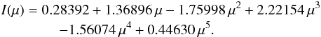 (1)
(1) -
Differential rotation: we used the rotation law of the Sun as measured by Snodgrass & Ulrich (1990) with l the solar latitude and ν the angular sidereal velocity in degrees per day (see Schroeter 1985, for a discussion of solar differential rotation and of observational challenges of solar velocity field measurements):
 (2)Because of the orbital motion of Earth, we converted
from sidereal into synodic rotation velocity:
(2)Because of the orbital motion of Earth, we converted
from sidereal into synodic rotation velocity: 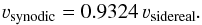 (3)
(3) -
Convective blueshift: granular motion introduces velocity fluctuations of the photosphere plasma in horizontal and vertical direction. The correlation between velocity and temperature (intensity) produces systematic Doppler shifts that vary over the solar disk (Beckers & Nelson 1978; Gray 2009). In general, the effect is quite well understood and can be modeled in (magneto-) hydrodynamic simulations (e.g., Beeck et al. 2013). However, the blueshift can vary between different spectral lines and sensitively depends on solar limb angle and the presence of magnetic fields because convection is suppressed in sunspots and magnetically active regions. Reference observations of the effect require very high wavelength accuracy and knowledge about the position on the solar surface to correct for Doppler shifts from solar rotation; such observations are available for one position 10′′ from the solar limb in Stenflo (2015), but were measured at limited wavelength accuracy (see Reiners et al. 2016). We parameterized the convective blueshift as a function of the solar limb angle μ using a sigmoid function. The parameters of the function are chosen to qualitatively follow convective blueshift as shown in Fig. 18 of Beeck et al. (2013) for the Sun, and to provide a reasonable fit in the RM curve. Our parameterization is shown in Fig. 2, it is neither an accurate reproduction of any model simulation nor the result of a systematic fit to the observed RVs. The purpose of this parameterization is to demonstrate the influence of convective blueshift on the RM curve. Nevertheless, we extensively tried to find parameterizations that provide a better fit to the RV curve, but with limited success.
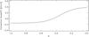 |
Fig. 2 Parameterization of convective blueshift as a function of solar limb angle. The curve qualitatively reproduces results from 3D magneto-hydrodynamic simulations and provides a useful fit to the observed RV curve; see text for details. |
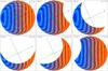 |
Fig. 3 Eclipse configuration in synthetic Dopplergram. Colors show the velocity projected toward the observer; the color coding is the same as in the middle panel of Fig. 4 with velocities between −3 and + 3 km s-1 from blue to red with yellow stripes. Universal time and fraction of the surface occulted by the Moon are given in the upper left and upper right part of the images, respectively. Orientation on sky is shown as the black coordinate system, the green line shows the orientation of the horizon at any given time. White circles in the upper left panel show solar limb angles of μ = 0.8,0.6 and μ = 0.3. |
The color-coding of radial velocity reveals an interesting feature: the combination of latitudinal differential rotation and convective blueshift leads to almost vertical lines of equal RV for most of the central part of the solar disk. At low μ-values, toward the limb of the Sun, lines of equal RV show a strong gradient toward the left in the plot, which is caused by the relative redshift at low μ, that is, velocities close to the limb become suddenly redshifted on the projected solar disk (cf. Fig. 2).
During eclipse, the Moon occulted the solar disk from the west, that is, from the redshifted side of the velocity distribution. The RM curve therefore first showed RVs distorted to the blue. This is different from the canonical picture in stars that are orbited by planets whose orbital motion is in the same direction as the stellar rotation. In the Sun-Earth-Moon system, this is caused by the fact that all orbital and angular velocities point in the same direction, but we observe the Moon occulting the Sun while orbiting Earth.
5.3. Solar surface observations
An alternative, empirical description of the solar velocity fields and their magnetism can be derived directly from solar observations, for example, from images taken by the Helioseismic and Magnetic Imager (HMI; Schou et al. 2012) onboard the Solar Dynamics Observatory (SDO; Pesnell et al. 2012). We downloaded images of intensity, Doppler velocities, and the magnetogram taken on March 20, 2015, at 09:36:00 UT with HMI from JSOC3. Exposure times were 720 s. The images are shown in Fig. 4 at the typical resolution of our RV calculations (see below).
In the intensity image, solar limb darkening and spots are visible. The Dopplergram shows a similar structure as the parameterized model, but also much more small-scale structure from noise or granulation. The magnetogram reveals the magnetic areas of opposite polarity near the equator. The magnetogram allows us to test scenarios with convective blueshift suppressed at certain magnetic field strengths. We discuss this in Sect. 6.
Dopplergrams were used before to infer information about the effect of solar granulation and active regions on solar RV measurements (e.g., Meunier et al. 2010b; Haywood et al. 2016). So far, it has never been shown that the RV variations deduced from solar Dopplergrams are quantitatively similar to disk-integrated RV observations. We argue that HMI Dopplergrams are not a useful source of information for accurate RVs because (i) Dopplergrams exhibit a number of systematic effects across the solar disk that can introduce errors of up to a few 100 m s-1 between different areas on the disk; (ii) there is a significant systematic difference between the observation of a stellar or solar disk-integrated RV and the integration of Dopplergram RVs for individually resolved disk areas (the canonical way to disk-integrate Dopplergram information is to use intensity to weight individual surface areas. This approach neglects the difference in line profiles across the solar disk, which introduces a second mechanism of weighting between surface elements); and (iii) the calculation of velocities across the solar disk relies on a number of filters across one spectral line, but the line shape varies across the disk, with the result that information from the limb and disk center cannot directly be compared without introducing errors much larger than several 10 m s-1. These effects are described in Fleck et al. (2011), Schou et al. (2012), Couvidat et al. (2012a,b), and Welsch et al. (2013). A velocity map showing typical instrumental effects and other systematic flow fields in HMI Doppler maps is shown in Löhner-Böttcher & Schlichenmaier (2013).
A visual comparison between our synthetic Dopplergram (upper left panel in Fig. 3) and the observed HMI Dopplergram (middle panel in Fig. 4) reveals some striking differences. First, the vertical yellow stripes only show very little curvature in the synthetic images (Fig. 3), but they are significantly curved in the observed Dopplergram (Fig. 4). Most important is the difference very close to the limb; at limb angles <0.6 the surface areas in the synthetic Dopplergrams show a sudden increase in Doppler velocities to the red (more positive velocities closer to the limb). This is visible in the knee of the yellow stripes at around μ = 0.6 and is caused by our parameterization of convective blueshift seen in Fig. 2. Although the data appear more fine-structured in the HMI Dopplergram, this trend clearly is much weaker in the Dopplergram, meaning that the blueshift adopted in our model is not entirely seen in HMI observations. We show below that the solar RV curve confirms the relevance of this convective blueshift for disk-integrated solar observations.
5.4. Radial velocity calculation
We calculated Sun-as-a-star radial velocities by integrating over the visible surface disk. We divided the solar surface into segments of equal area. For our calculations, we segmented the surface into 50 830 segments of equal area of which 25 417 were visible as long as the Sun was not occulted by the Moon. The inclination of the Sun during our observations was i = 97.05° 4.
For each surface segment, we computed the velocity at the center of the segment and weighted its contribution by the projected size and intensity according to limb darkening and extinction. The segment’s projected velocity was calculated from the solar rotation law and convective blueshift. At the angular size of the Sun of almost half a degree, extinction and barycentric velocity significantly differ across the solar disk. We computed the barycentric correction for each individual segment with values of right ascension and declination computed for the center of each segment. We verified that the barycentric correction from JPL emphemeris for the center of the Sun agreed with our results.
Extinction describes the effect of intensity attenuation caused by Earth’s atmosphere. Attenuation can be described with the formula  (4)with k the extinction coefficient and x airmass; typical extinction coefficients are between 0.1 and 0.6 for visual wavelengths. We can estimate the effect of extinction on the solar RV curve from Fig. 3; extinction is stronger for regions on the solar disk located at higher airmass, that is, below the green lines. At maximum eclipse (09:42 UT), the orientation of the horizon was almost perpendicular to the rotation axis of the Sun, while the line connecting Sun and Moon is almost parallel to the rotation axis. This led to a degeneracy between the effects from extinction and velocity fields during eclipse without consequences for our calculations.
 |
Fig. 4 HMI images taken at 09:36 UT, exposure time 720 s, shown at the resolution of our simulations. Left: intensity showing empirical limb darkening and a small sunspot at NE; middle: Dopplergram shown with the same color code as in Fig. 3; right: magnetogram showing positive (white) and negative (black) magnetic polarities. |
The value of the extinction coefficient is unknown but constrained by the total intensity visible during the entire observation (Fig. 1). We tested the influence of extinction and found that its value did not significantly influence the shape of the RM curve (for realistic values of k). We used an extinction coefficient of 0.4 for the beginning of the observations that linearly diminishes in time to 0.1 at the end of observations. In the wavelength range that we used to calculate the flux (5500–6000 Å), 0.1 is a reasonable value for good weather conditions as during the end of our observations. At the beginning of our observations, the Sun was just rising, and ice crystals were probably still affecting extinction at very high airmass. Our model can reproduce the observed flux in Fig. 1 very well, differences like those between 08:00 and 08:30 UT are probably caused by variable extinction and/or thin clouds.
To compute the final RV, we can chose between different strategies. The easiest (and by far the fastest) way is to calculate the average of the radial velocities of all visible surface segments weighted by their intensity, taking into account limb darkening and extinction (as done in models 1, 2, and 4 below). A second strategy is to compute the line profile for each segment, shift it according to the segment radial velocity, add all the segment line profiles weighted by intensity, and determine the RV of the final line profile (model 3). This strategy can account for the problem that the RV calculation may be affected by asymmetries in the final line profile that can arise from the asymmetric velocity distribution of the surface segments because of convective blueshift and the eclipse. It can also take different line profiles for different solar limb angles and intrinsically asymmetric lines into account. We tested both strategies and present the results in the following.
6. Results
6.1. Rossiter-McLaughlin curve
We calculated the RM curve using four different models: model 1 averages velocities across the solar disk including no convective blueshift; model 2 is the same, but includes convective blueshift. Model 3 uses the full calculation of line profiles, and model 4 again is similar to models 1 and 2, but uses velocity fields taken from satellite observations.
6.1.1. Standard line model
Our first calculation of the RV curve, model 1, follows the simplest approach; we parameterized limb darkening and solar differential rotation as introduced in Sect. 5.2, and we calculated RVs from the weighted velocities of all visible segments, that is, we did not compute any line profiles. In this first attempt, convective blueshift was not taken into account. We show the results of this calculation and a comparison to our observations and to solar barycentric velocities from JPL’s ephemeris in Fig. 5: in the top panel, we show our RV observations (black symbols) together with the results from the first model (red line). The dashed gray line shows our model results for the unobscured solar disk (no eclipse). The blue line shows solar velocities as taken from JPL’s ephemeris. For our plots, we decided to show the JPL emphemeris and our solar RV observations with no additional RV offset. However, for better comparison between our eclipse model (red line) and solar RV observations, we applied an offset to the eclipse model. In model 1, without convective blueshift, our eclipse by design reproduces the JPL ephemeris. The offset between the two is only 30 cm s-1. The offset between JPL ephemeris and solar RV observations is 94 m s-1, hence the solid red and dashed gray lines in Fig. 5 are offset by that amount. This offset is partly caused by inaccuracies of our optical system (see Lemke & Reiners 2016), but we expect a systematic error of only a few ten m s-1. The bulk of the difference between ephemeris and solar observations (94 m s-1) is caused by the real difference between the two mechanisms that affect integrated solar RV observations: net convective blueshift and gravitational redshift. Our observations indicate that the sum of both effects is on the order of 90–100 m s-1, but the uncertainties are large (see above). This value could be determined with higher accuracy if the systematic uncertainties of our optical setup were better understood. Such a measurement would allow the direct determination of the net convective blueshift because the gravitational redshift is known to relatively high accuracy (Lindegren & Dravins 2003).
The comparison between observations, JPL ephemeris, and our model calculations shows that the main ingredients of the eclipse RV observations are captured by our model. The barycentric motion of the Sun varies by roughly 300 m s-1 during our observations. The RM effect produces an asymmetric curve with amplitudes between −500 m s-1 and + 800 m s-1 in addition to barycentric motion. In this first model without convective blueshift, the calculated RM curve appears systematically offset toward the blue. The bottom panel of Fig. 5 shows the residuals between RV observations and the model results. The difference during transit is clearly visible, reaching almost 100 m s-1 during eclipse center. We ascribe the main part of this difference to convective blueshift.
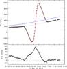 |
Fig. 5 Observations of solar RVs during the eclipse together with the standard line model 1. Top panel: black plus symbols show our solar RV observations. The red line shows results from our model corrected for an offset so that they match observations after the end of the eclipse (see text). The gray dashed line shows the eclipse-free model (only barycentric motion). The blue line shows barycentric motion from JPL’s ephemeris. Bottom panel: residuals between observations and model (black symbols minus red curve in top panel). |
During the first 1.5 h before the eclipse, our RVs show a systematic trend that is visible as residual starting at 30 m s-1 at 07:00 UT and approaching zero difference after 08:30 UT, just when the eclipse begins. Such an effect is not visible after the eclipse, residuals after 11:00 UT scatter closely around zero. We ascribe this effect to the systematic problem of our optical setup. We showed in Lemke & Reiners (2016) that RV trends of this amplitude were found in other observations, probably caused by a systematic problem with the way we couple sunlight into the fiber. The linear slope of the residual before 08:30 UT is very similar to what we see in other observations. Unfortunately, we cannot exclude that similar effects occurred during eclipse or after, but we only expect effects that would be detected as linear trends or sudden jumps in the residuals. We do not see clear evidence of such effects. Thus, we assume for the following that the trend we see before 08:30 UT is caused by our optical setup and that no such effect occurs later during observation. It is suspicious that the trend stops exactly at the beginning of the eclipse, but the residuals give no reason to believe that there is a significant effect at any time later during our observations. In the comparisons to our other models, we correct for this linear slope from now on by division through a straight fit to the data before 08:30 UT.
After correcting for this trend, we were able to measure the scatter of our solar RV measurements outside eclipse. We found that before and after eclipse (81 observations) our RV values scatter around the barycentric trend with an rms of 2.2 m s-1. The cadence of these observations is 97 s, which means that part of this scatter is probably caused by solar oscillations. After averaging our measurements into ~5 min bins (averaging three exposures, 27 bins), we found that our RV measurements scatter with an rms of 1.6 m s-1. Further binning reduced the scatter even more: binning five exposures into 16 data points yielded an rms of 1.25 m s-1, and ten exposures with 8 data points yielded 0.7 m s-1. The scaling of the rms scatter with bin size follows expectation from purely statistical scatter. We conclude that our data points outside eclipse are not systematically affected by trends other than the linear trend discussed above. The statistical nature of the RV scatter could be caused by solar short-term variability or by the statistical noise in our RV measurements. Our estimate from photon noise is on the order of only 10 cm s-1. We therefore suspect that the source of the RV “noise” in our observations of the Sun as a star is in fact solar granulation.
6.1.2. Standard line model with convective blueshift
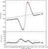 |
Fig. 6 Observations of solar RVs during the eclipse together with results from model 1 including convective blueshift. Lines and symbols are the same as in Fig. 5. Here, the model velocities (red line) match the solar observations without any offset. |
In model 2 we used the same strategy to calculate solar RVs as in model 1, but added the parameterization of convective blueshift as shown in Fig. 2. The results are shown in Fig. 6. Lines and symbols are the same as in Fig. 5, the model RVs (red line) are not offset, but their absolute velocities match the solar RV observations because the offset is one parameter for the blueshift velocities. As explained above, we do not claim that our parameterization provides absolute values for the blueshift because there may be systematic offsets in our observations. More important than the absolute RV calibration is that the calculated RVs provide a significantly better match to the observations than the model without blueshift; phenomenologically, the modeled RM curve is shifted to redder velocities. The residuals between calculated and observed RVs during eclipse are still fairly high, up to 40 m s-1 early during eclipse, but they are lower later.
We noted in Sect. 2 that the time of our observations is unknown within several 10 s because of an offset in our instrument clock. This means we have the freedom to shift the observations in time by several 10 s. Boundary conditions for the time correction are that the calculated values must match the flux variations as shown in Fig. 1 and the RVs. There is some degeneracy between the time and the amount of blueshift at least during the center of eclipse. Better information comes from the peaks in the RM curve and the time of ingress and egress. We have extensively tested other parameterizations of blueshift and combinations of blueshift and time-offsets; our parameterization of blueshift together with an offset of 50 s applied to the time of our observations provides the RV curve as shown. We were not able to produce a significantly better match to the data using any other set of parameters. We conclude that the introduction of convective blueshift is key to the understanding of the solar eclipse RV curve. Nevertheless, residuals are still significant, and we see no way to produce better RV calculations with this type of model.
6.1.3. Line profile model
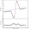 |
Fig. 7 Observations of solar RVs during the eclipse together with results from model 3 involving the calculation of line profiles and determination of RVs from the profiles. |
In our third model we calculated specific line profiles for every segment on the visible solar surface. For that, we interpolated ten synthetic line profiles of the Fe I line at 6173 Å from Beeck et al. (2013) calculated at values of μ = 0.1,0.2,...1.0, and assigned a line profile to every surface segment (see also Sect. 6.2 and Fig. 11). We shifted every line profile according to the rotational Doppler velocity of each segment and calculated a disk-integrated line profile with respect to limb darkening and extinction. From this profile, we calculated the RV as done for the solar observations. The potential advantages of this approach are that line asymmetries and convective blueshift as functions of limb angle are correctly included and that any systematic effects from the way how RVs are calculated are captured.
The results from model 3 are shown in Fig. 7 in the same fashion as before. The mean velocities from our calculations are offset by −130 m s-1 with respect to the solar RV observations. This is not critical because the MHD simulations were not designed to absolutely match observed solar wavelengths. The residuals between the calculated RV curve and solar observations are somewhat lower than the residuals calculated from the simpler model 2 (a maximum of 30 m s-1 instead of 40 m s-1), but the qualitative discrepancy during eclipse still exists. The relative mismatch is always smaller than 10%, which is a reasonably good match. Nevertheless, the calculation of more realistic line profiles and the calculation of RVs from profiles instead of simple weighted velocities did not significantly improve the final RV model. This may not be surprising because our parameterization of convective blueshift in model 2 was derived from the line profiles we used in model 3, and therefore most of the information was already included. On the other hand, it implies that the way the RVs are calculated is not the reason for the discrepancy and that a probably more fundamental problem exists in our description of the solar surface spectra across the solar disk. As a main candidate, we suggest the shape of line profiles as a function of solar limb angle μ.
6.1.4. Solar velocity fields from HMI observations
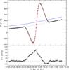 |
Fig. 8 Observations of solar RVs during the eclipse together with results from model 4 adopting limb darkening and solar surface velocities from HMI observations. Lines and symbols are the same as in Fig. 5. |
In our fourth model, we adopted limb darkening and solar velocity fields from HMI observations (Fig. 4), RVs were calculated as in our first two models. With this model, we wished to test the information contained in HMI Dopplergrams. We inspected the limb-darkening law seen in the HMI images and confirm that it is very similar to the parameterization we used earlier. It made no significant difference whether we used information on limb darkening from the HMI images or from the parameterization. For consistency, we used the image information in model 4. The resulting RV curve is shown in Fig. 8, it is very similar to our first model, in which limb darkening and rotational velocities were parameterized, but no convective blueshift was applied. This could either mean that our parameterization of convective blueshift is incorrect, or that HMI Dopplergrams do not capture the information relevant for full-disk surface integration. Our convection model appears to be the better choice because (a) we obtain a much better match to the observed solar RM curve; and (b) the results from full line-profile calculations (model 3) are very similar to the RVs, including our convection model.
Our test in model 4 revealed a relevant result: it shows that when the HMI Dopplergram is used to calculate an intensity-weighted surface-integration to construct disk-integrated solar RVs, the result is similar to including only solar surface differential rotation, but it lacks most of the information about convective blueshift. This may be partly due to the uncertainty of Dopplergram velocities, in particular when Doppler velocities are compared across the full solar disk (Couvidat et al. 2012a,b; Welsch et al. 2013). A more important explanation probably is that the way the Dopplergrams are constructed differs from the definition of RVs as used in our model calculations (Schou et al. 2012); Dopplergram velocities are calculated from several filters around the Fe I line at 6713 Å, which implies that they reflect a certain velocity field according to the effective formation height, which may not coincide with the height we observe in our data (Fleck et al. 2011). To test the reliability of our spectroscopic RV data and its relation to the 6173 Å line, we computed RVs from our spectra using only this line. The results were of course more noisy, but we found excellent agreement between results from our broad-band spectra and those using only this single line. We conclude that the choice of the line does not cause any bias in the comparison between our RV determination and the HMI Dopplergrams, and that the Dopplergram velocity fields, if used in this way to construct RVs, capture the differential rotation of the Sun quite well, but not the pattern of convective blueshift.
Another test we performed involves information about the solar magnetic field. It is often assumed that magnetic fields stronger than a particular value suppress convective blueshift and that relevant RV variations in solar observations can be explained by blueshift suppressed in sunspots. For long-term observations, this works through corotation and evolution of magnetically active regions, but long-term evolution of RVs and solar active regions cannot be assessed with our observations. Our attempts to improve the RV model by applying lower blueshifts in regions of high magnetic fields were all fruitless; we found no improvement to our RV curve when we modified the blueshift pattern in regions of high magnetic fields. In particular, varying the blueshift in the region of the visible spot did not significantly influence the RV curve.
6.2. Line profiles
Our observations equipped us with a way to compare our synthetic line profiles to empirical data not only for spectra from the full disk-integrated solar surface, in which much of the limb angle information is lost, but also for spectra integrated over only parts of the disk while other parts were eclipsed by the Moon.
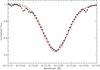 |
Fig. 9 Comparison of unperturbed line profiles; black circles: observed solar spectrum outside transit; gray dashed line: solar atlas; red solid line: modeled line profile for the entire solar disk. Telluric lines appear at λ = 6173.2–6173.25 Å and 6173.45 Å in the observations but are averaged out in the solar atlas. |
A comparison between the fully disk-integrated spectrum for the observed Sun and the line profile model for the 6173 Å line (from model 3) is shown in Fig. 9. In this figure we show a calculated profile together with a spectrum taken during our observations before transit with black dots, and the line from the solar atlas of Reiners et al. (2016). The latter was constructed from many individual exposures taken at very different barycentric velocities. The quality of this spectrum is much higher, and it is virtually free of telluric lines. The two observed solar spectra compare very well within the uncertainties. As a red solid line we show the result of the disk-integration of our 3D-MHD synthetic line profiles. The differences between model and observations are small but significant, they are on the order of 0.02–0.03 in normalized flux units. There is an obvious difference between the overall line shape of the observed and modeled profiles, which probably stems from larger differences between real and modeled line profiles at certain positions on the solar disk.
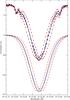 |
Fig. 10 Comparison between observed (top panel) and modeled (bottom panel) line profiles. In each panel, spectra at four different phases are shown: (1) before the eclipse (black solid lines); (2) during the first half of the eclipse (blueshifted red dashed lines); (3) during eclipse maximum (blue dashed lines); and (4) during the second half of the eclipse (redshifted red dashed lines). The configurations of the four phases are shown in Fig. 3. |
With our eclipse observations we can test the hypothesis that differences between synthetic and observed spectra are more severe in smaller regions of the solar disk. We show a comparison of modeled and observed spectra during different phases of the eclipse in Fig. 10. For each case, we show four different spectra: (1) a spectrum out of eclipse; (2) a spectrum taken at a phase when about 60% of the disk is occulted by the Moon, most of the visible part is on the blueshifted side of the Sun (spectrum taken at 09:24 UT, see upper right panel in Fig. 3); (3) a spectrum taken at eclipse maximum, the visible is almost symmetrically distributed between the blue- and redshifted parts of the disk (09:42 UT, lower left panel in Fig. 3); and (4) a spectrum like in (2), but after eclipse maximum and most of the visible disk red-shifted (10:00 UT, bottom middle panel in Fig. 3).
The comparison in Fig. 10 shows that out of eclipse and during eclipse maximum, the observed and modeled spectra compare quite well. The spectrum taken at eclipse maximum has a shallower core and wider wings than the spectrum taken out of eclipse. This behavior is well reproduced by our model. The two spectra observed during the first and second half of the eclipse (red dashed lines) are blue- and redshifted, respectively, and they both show a line core depth between the spectra taken out of eclipse and at eclipse maximum. In contrast to this, the modeled line profiles at these phases are significantly deeper. There is almost no difference between the line depth of these profiles and the spectrum modeled out of eclipse. This is a clear discrepancy to our observations that we ascribe to incorrectly modeled line depths, in particular at intermediate μ-values (μ> 0.6), because at eclipse maximum mostly regions with lower μ-values are visible. Here, the calculated line depth seems to reproduce the observations quite well.
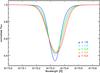 |
Fig. 11 Synthetic line profiles for solar surface areas at different μ-values from Beeck et al. (2013). |
To shed some light on the question whether incorrectly modeled line depths at intermediate μ-values can be the reason for the discrepancy between our observed eclipse spectra and our model, we show the synthetic line profiles from Beeck et al. (2013) in Fig. 11. The strong blueshift of the line at μ = 1 is clearly visible relative to the other line profiles. Furthermore, the μ = 1 profile is rather narrow but much deeper than all other profiles, and the line depths show a steep gradient from μ = 1 to μ = 0.6. A detailed investigation of possible uncertainties in the modeled line profiles is beyond the scope of this paper. Nevertheless, we note that the fast change of line depth at limb angles between μ = 0.6 and μ = 1 could imply that line depths for individual limb angles may be somewhat uncertain, or that our interpolation between the calculated profiles is incorrect. In any case, a detailed comparison between model spectra and observations at well-defined limb angles, in particular between μ = 0.6 and μ = 1, would be highly desirable.
7. Summary
On March 20, 2015, we obtained 159 high-resolution FTS spectra of the Sun as a star, 76 of them during partial solar eclipse. From each spectrum, we derived the apparent absolute RV. Before and after the eclipse, our RVs are tracking barycentric motion. During eclipse, they provide an exquisite benchmark RM curve with a peak-to-peak amplitude of almost 1.4 km s-1. The geometry of the event is fully determined by our knowledge about solar, lunar, and terrestrial motion. Doppler velocities on the solar surface and limb darkening are also well known, but information about the limb angle dependence of solar convective blueshift and spectral line shape is incomplete. With this paper, we publish the RV values of our observations. The time series can be used to test line profile calculations and codes calculating RM curves for exoplanet observations. The amplitude of the RM curve is orders of magnitudes higher than in typical exoplanet observations, while the uncertainties in the RVs are very small (S/N> 1000). In contrast to other stars, much information is available about solar surface velocities.
We tested whether we were able to reproduce the RM curve during solar eclipse using a set of different approaches. First, we parameterized limb darkening and solar surface rotation using standard descriptions but neglected convective blueshift. We calculated surface integrated RVs by computing the intensity-weighted average of the radial velocities over the visible solar disk. This first attempt resulted in an RV curve that qualitatively matched the observations, but revealed a clear offset with the RM curve being off to the blue. In our second model, we included a qualitative prescription of convective blueshift leaving all other steps as in our first model. This resulted in a much better reproduction of the observed RV curve, but still revealed residuals as high as 40 m s-1 especially during the first half of the eclipse. In our model 3 we calculated spectral line profiles for different locations on the solar surface and computed a disk-integrated line from which we determined the apparent solar RVs like in our observations. For the line profiles, we used results from a 3D-MHD calculation that inherently includes information on convective blueshift and the variation of the profile shape. While this model provided the best match to our observations, residuals were still as high as 30 m s-1, the relative errors were smaller than 10%. As a consistency check, we used solar surface observations from HMI in model 4 to describe limb darkening and solar velocity fields. The results of this exercise are very similar to those from model 1. This showed the limitation of the HMI Dopplergrams for full solar disk calculations. It is relevant for investigations of convective blueshift that use Dopplergram observations as reference (e.g., Meunier et al. 2010b; Haywood et al. 2016, using SOHO/MDI and SDO/HMI, respectively).
With the goal to identify the reason for the mismatch between our models and the RV observations, we inspected the line profiles modeled and observed during different phases of the eclipse. We found a mismatch of line depths close to phases 0.25 and 0.75, but a rather good match at phase 0.5 and outside eclipse. We concluded that the line depths at intermediate limb angles, μ between 0.6 and 1, may be systematically overestimated, which could lead to an incorrect weighting of velocities across the solar disk. Identifying reasons for this problem is beyond the scope of this work, but we see the need to obtain high-quality spectral observations of the solar surface at well-defined limb angles with high wavelength accuracy.
As the main cause for the mismatch between our model calculations and observed RVs, we identified our limited knowledge about line profiles and convective blueshift as a function of solar limb angle. Alternative explanations include the variation of blueshift with magnetic field strength, incorrect assumptions about solar rotation and granulation, and so far undiscovered mechanisms affecting the spectral observation of the spatially extended solar disk during eclipse. The solution of this puzzle will have ramifications for solar physics because a better understanding of the local line profiles is required, and for exoplanet research because it will lead to a more accurate description of the RM curve in particular, and of stellar RVs in general.
Latitude: 51°33′38.1″ N; longitude: 009°56′39.6″ E; altitude: 201 m.
Acknowledgments
We thank Jasper Schou, Achim Gandorfer, and Mathias Zechmeister for helpful discussions, and the team at IAG for their support with the observations. Part of this work was supported by the ERC Starting Grant Wavelength Standards, Grant Agreement Number 279347. A.R. acknowledges research funding from DFG grant RE 1664/9-1. The FTS was funded by the DFG and the State of Lower Saxony through the Großgeräteprogramm Fourier Transform Spectrograph.
References
- Anglada-Escudé, G., & Butler, R. P. 2012, ApJS, 200, 15 [NASA ADS] [CrossRef] [Google Scholar]
- Anglada-Escudé, G., Tuomi, M., Arriagada, P., et al. 2016, ApJ, 830, 74 [NASA ADS] [CrossRef] [Google Scholar]
- Beckers, J. M., & Nelson, G. D. 1978, Sol. Phys., 58, 243 [NASA ADS] [CrossRef] [Google Scholar]
- Beeck, B., Cameron, R. H., Reiners, A., & Schüssler, M. 2013, A&A, 558, A49 [NASA ADS] [CrossRef] [EDP Sciences] [Google Scholar]
- Boué, G., Montalto, M., Boisse, I., Oshagh, M., & Santos, N. C. 2013, A&A, 550, A53 [NASA ADS] [CrossRef] [EDP Sciences] [Google Scholar]
- Cegla, H. M., Lovis, C., Bourrier, V., et al. 2016a, A&A, 588, A127 [NASA ADS] [CrossRef] [EDP Sciences] [Google Scholar]
- Cegla, H. M., Oshagh, M., Watson, C. A., et al. 2016b, ApJ, 819, 67 [NASA ADS] [CrossRef] [Google Scholar]
- Couvidat, S., Rajaguru, S. P., Wachter, R., et al. 2012a, Sol. Phys., 278, 217 [NASA ADS] [CrossRef] [Google Scholar]
- Couvidat, S., Schou, J., Shine, R. A., et al. 2012b, Sol. Phys., 275, 285 [NASA ADS] [CrossRef] [Google Scholar]
- Del Moro, D. 2004, A&A, 428, 1007 [NASA ADS] [CrossRef] [EDP Sciences] [Google Scholar]
- Deming, D., & Plymate, C. 1994, ApJ, 426, 382 [Google Scholar]
- Deming, D., Espenak, F., Jennings, D. E., Brault, J. W., & Wagner, J. 1987, ApJ, 316, 771 [NASA ADS] [CrossRef] [Google Scholar]
- Dravins, D., Ludwig, H.-G., Dahlen, E., & Pazira, H. 2015, in 18th Cambridge Workshop on Cool Stars, Stellar Systems, and the Sun, eds. G. T. van Belle, & H. C. Harris, 853 [Google Scholar]
- Dumusque, X., Boisse, I., & Santos, N. C. 2014, ApJ, 796, 132 [NASA ADS] [CrossRef] [Google Scholar]
- Dumusque, X., Glenday, A., Phillips, D. F., et al. 2015, ApJ, 814, L21 [NASA ADS] [CrossRef] [Google Scholar]
- Fabrycky, D. C., & Winn, J. N. 2009, ApJ, 696, 1230 [NASA ADS] [CrossRef] [Google Scholar]
- Fischer, D. A., Anglada-Escude, G., Arriagada, P., et al. 2016, PASP, 128, 066001 [NASA ADS] [CrossRef] [Google Scholar]
- Fleck, B., Couvidat, S., & Straus, T. 2011, Sol. Phys., 271, 27 [NASA ADS] [CrossRef] [Google Scholar]
- Gaudi, B. S., & Winn, J. N. 2007, ApJ, 655, 550 [NASA ADS] [CrossRef] [Google Scholar]
- Gray, D. F. 2009, ApJ, 697, 1032 [NASA ADS] [CrossRef] [Google Scholar]
- Hatzes, A. P. 2013, ApJ, 770, 133 [NASA ADS] [CrossRef] [Google Scholar]
- Haywood, R. D., Collier Cameron, A., Unruh, Y. C., et al. 2016, MNRAS, 457, 3637 [NASA ADS] [CrossRef] [Google Scholar]
- İz, H., Ding, X., Dai, C., & Shum, C. 2011, J. Geodetic Sci., 1, 348 [NASA ADS] [Google Scholar]
- Jimenez, A., Palle, P. L., Regulo, C., Roca Cortes, T., & Isaak, G. R. 1986, Adv. Space Res., 6, 89 [NASA ADS] [CrossRef] [PubMed] [Google Scholar]
- Kurucz, R. 1993, ATLAS9 Stellar Atmosphere Programs and 2 km s-1 grid, Kurucz CD-ROM (Cambridge, Mass.: Smithsonian Astrophysical Observatory), 13 [Google Scholar]
- Lagrange, A.-M., Desort, M., & Meunier, N. 2010, A&A, 512, A38 [NASA ADS] [CrossRef] [EDP Sciences] [Google Scholar]
- Lemke, U., & Reiners, A. 2016, PASP, 128, 095002 [NASA ADS] [CrossRef] [Google Scholar]
- Lindegren, L., & Dravins, D. 2003, A&A, 401, 1185 [NASA ADS] [CrossRef] [EDP Sciences] [Google Scholar]
- Livingston, W. C. 1982, Nature, 297, 208 [NASA ADS] [CrossRef] [Google Scholar]
- Löhner-Böttcher, J., & Schlichenmaier, R. 2013, A&A, 551, A105 [NASA ADS] [CrossRef] [EDP Sciences] [Google Scholar]
- Marchwinski, R. C., Mahadevan, S., Robertson, P., Ramsey, L., & Harder, J. 2015, ApJ, 798, 63 [NASA ADS] [CrossRef] [Google Scholar]
- McLaughlin, D. B. 1924, ApJ, 60, 22 [NASA ADS] [CrossRef] [Google Scholar]
- McMillan, R. S., Moore, T. L., Perry, M. L., & Smith, P. H. 1993, ApJ, 403, 801 [NASA ADS] [CrossRef] [Google Scholar]
- Meunier, N., Desort, M., & Lagrange, A.-M. 2010a, A&A, 512, A39 [NASA ADS] [CrossRef] [EDP Sciences] [Google Scholar]
- Meunier, N., Lagrange, A.-M., & Desort, M. 2010b, A&A, 519, A66 [NASA ADS] [CrossRef] [EDP Sciences] [Google Scholar]
- Molaro, P., Monaco, L., Barbieri, M., & Zaggia, S. 2013, MNRAS, 429, L79 [NASA ADS] [CrossRef] [Google Scholar]
- Molaro, P., Barbieri, M., Monaco, L., Zaggia, S., & Lovis, C. 2015, MNRAS, 453, 1684 [NASA ADS] [CrossRef] [Google Scholar]
- Neckel, H., & Labs, D. 1994, Sol. Phys., 153, 91 [NASA ADS] [CrossRef] [Google Scholar]
- Ohta, Y., Taruya, A., & Suto, Y. 2005, ApJ, 622, 1118 [NASA ADS] [CrossRef] [Google Scholar]
- Pesnell, W. D., Thompson, B. J., & Chamberlin, P. C. 2012, Sol. Phys., 275, 3 [NASA ADS] [CrossRef] [Google Scholar]
- Reiners, A., Mrotzek, N., Lemke, U., Hinrichs, J., & Reinsch, K. 2016, A&A, 587, A65 [NASA ADS] [CrossRef] [EDP Sciences] [Google Scholar]
- Robertson, P., Mahadevan, S., Endl, M., & Roy, A. 2014, Science, 345, 440 [NASA ADS] [CrossRef] [Google Scholar]
- Robertson, P., Roy, A., & Mahadevan, S. 2015, ApJ, 805, L22 [NASA ADS] [CrossRef] [Google Scholar]
- Rossiter, R. A. 1924, ApJ, 60 [Google Scholar]
- Schou, J., Scherrer, P. H., Bush, R. I., et al. 2012, Sol. Phys., 275, 229 [Google Scholar]
- Schroeter, E. H. 1985, Sol. Phys., 100, 141 [NASA ADS] [CrossRef] [Google Scholar]
- Shporer, A., & Brown, T. 2011, ApJ, 733, 30 [NASA ADS] [CrossRef] [Google Scholar]
- Snodgrass, H. B. 1992, in The Solar Cycle, ed. K. L. Harvey, ASP Conf. Ser., 27, 205 [Google Scholar]
- Snodgrass, H. B., & Ulrich, R. K. 1990, ApJ, 351, 309 [Google Scholar]
- Stenflo, J. O. 2015, A&A, 573, A74 [NASA ADS] [CrossRef] [EDP Sciences] [Google Scholar]
- Takeda, Y., Ohshima, O., Kambe, E., et al. 2015, PASJ, 67, 10 [NASA ADS] [Google Scholar]
- Torres, G., Winn, J. N., & Holman, M. J. 2008, ApJ, 677, 1324 [NASA ADS] [CrossRef] [Google Scholar]
- Welsch, B. T., Fisher, G. H., & Sun, X. 2013, ApJ, 765, 98 [NASA ADS] [CrossRef] [Google Scholar]
Appendix A: Additional tables
Log of observations.
All Tables
All Figures
|
Fig. 1 Upper panel: photographs of the solar eclipse taken at our observatory; middle panel: observed flux normalized to 1.0 at 11:00 UT, black open circles show flux integrated from our observed spectra, the red line shows the flux from our extinction model and eclipse (see text); bottom panel: airmass during our observations. Times are given in UT. |
| In the text | |
|
Fig. 2 Parameterization of convective blueshift as a function of solar limb angle. The curve qualitatively reproduces results from 3D magneto-hydrodynamic simulations and provides a useful fit to the observed RV curve; see text for details. |
| In the text | |
|
Fig. 3 Eclipse configuration in synthetic Dopplergram. Colors show the velocity projected toward the observer; the color coding is the same as in the middle panel of Fig. 4 with velocities between −3 and + 3 km s-1 from blue to red with yellow stripes. Universal time and fraction of the surface occulted by the Moon are given in the upper left and upper right part of the images, respectively. Orientation on sky is shown as the black coordinate system, the green line shows the orientation of the horizon at any given time. White circles in the upper left panel show solar limb angles of μ = 0.8,0.6 and μ = 0.3. |
| In the text | |
|
Fig. 4 HMI images taken at 09:36 UT, exposure time 720 s, shown at the resolution of our simulations. Left: intensity showing empirical limb darkening and a small sunspot at NE; middle: Dopplergram shown with the same color code as in Fig. 3; right: magnetogram showing positive (white) and negative (black) magnetic polarities. |
| In the text | |
|
Fig. 5 Observations of solar RVs during the eclipse together with the standard line model 1. Top panel: black plus symbols show our solar RV observations. The red line shows results from our model corrected for an offset so that they match observations after the end of the eclipse (see text). The gray dashed line shows the eclipse-free model (only barycentric motion). The blue line shows barycentric motion from JPL’s ephemeris. Bottom panel: residuals between observations and model (black symbols minus red curve in top panel). |
| In the text | |
|
Fig. 6 Observations of solar RVs during the eclipse together with results from model 1 including convective blueshift. Lines and symbols are the same as in Fig. 5. Here, the model velocities (red line) match the solar observations without any offset. |
| In the text | |
|
Fig. 7 Observations of solar RVs during the eclipse together with results from model 3 involving the calculation of line profiles and determination of RVs from the profiles. |
| In the text | |
|
Fig. 8 Observations of solar RVs during the eclipse together with results from model 4 adopting limb darkening and solar surface velocities from HMI observations. Lines and symbols are the same as in Fig. 5. |
| In the text | |
|
Fig. 9 Comparison of unperturbed line profiles; black circles: observed solar spectrum outside transit; gray dashed line: solar atlas; red solid line: modeled line profile for the entire solar disk. Telluric lines appear at λ = 6173.2–6173.25 Å and 6173.45 Å in the observations but are averaged out in the solar atlas. |
| In the text | |
|
Fig. 10 Comparison between observed (top panel) and modeled (bottom panel) line profiles. In each panel, spectra at four different phases are shown: (1) before the eclipse (black solid lines); (2) during the first half of the eclipse (blueshifted red dashed lines); (3) during eclipse maximum (blue dashed lines); and (4) during the second half of the eclipse (redshifted red dashed lines). The configurations of the four phases are shown in Fig. 3. |
| In the text | |
|
Fig. 11 Synthetic line profiles for solar surface areas at different μ-values from Beeck et al. (2013). |
| In the text | |
Current usage metrics show cumulative count of Article Views (full-text article views including HTML views, PDF and ePub downloads, according to the available data) and Abstracts Views on Vision4Press platform.
Data correspond to usage on the plateform after 2015. The current usage metrics is available 48-96 hours after online publication and is updated daily on week days.
Initial download of the metrics may take a while.