| Issue |
A&A
Volume 595, November 2016
|
|
|---|---|---|
| Article Number | A9 | |
| Number of page(s) | 15 | |
| Section | Interstellar and circumstellar matter | |
| DOI | https://doi.org/10.1051/0004-6361/201628859 | |
| Published online | 24 October 2016 | |
Sparse aperture masking interferometry survey of transitional discs⋆
Search for substellar-mass companions and asymmetries in their parent discs
1 University of Exeter, Astrophysics Group, School of Physics, Stocker Road, Exeter EX4 4QL, UK
e-mail: mwillson@astro.ex.ac.uk
2 Department of Astronomy, University of Michigan, 311 West Hall, 1085 South University Ave, Ann Arbor, MI 48109, USA
3 Research School of Astronomy & Astrophysics, Mount Stromlo Observatory Cotter Road, Weston Creek, ACT 2611, Australia
4 Department of Physics, University of Cincinnati, Cincinnati, OH 45221, USA
5 Space Science Institute, 475 Walnut St., Suite 205, Boulder, CO 80301, USA
6 Department of Astronomy, Boston University, 725 Commonwealth Avenue, Boston, MA 02215, USA
7 Harvard-Smithsonian Center for Astrophysics, 60 Garden Street, MS-78, Cambridge, MA 02138, USA
Received: 4 May 2016
Accepted: 14 July 2016
Context. Transitional discs are a class of circumstellar discs around young stars with extensive clearing of dusty material within their inner regions on 10s of au scales. One of the primary candidates for this kind of clearing is the formation of planet(s) within the disc that then accrete or clear their immediate area as they migrate through the disc.
Aims. The goal of this survey was to search for asymmetries in the brightness distribution around a selection of transitional disc targets. We then aimed to determine whether these asymmetries trace dynamically-induced structures in the disc or the gap-opening planets themselves.
Methods. Our sample included eight transitional discs. Using the Keck/NIRC2 instrument we utilised the Sparse Aperture Masking (SAM) interferometry technique to search for asymmetries indicative of ongoing planet formation. We searched for close-in companions using both model fitting and interferometric image reconstruction techniques. Using simulated data, we derived diagnostics that helped us to distinguish between point sources and extended asymmetric disc emission. In addition, we investigated the degeneracy between the contrast and separation that appear for marginally resolved companions.
Results. We found FP Tau to contain a previously unseen disc wall, and DM Tau, LkHα330, and TW Hya to contain an asymmetric signal indicative of point source-like emission. We placed upper limits on the contrast of a companion in RXJ 1842.9-3532 and V2246 Oph. We ruled the asymmetry signal in RXJ 1615.3-3255 and V2062 Oph to be false positives. In the cases where our data indicated a potential companion we computed estimates for the value of McṀc and found values in the range of 10−5−10−3 M2J yr−1.
Conclusions. We found significant asymmetries in four targets. Of these, three were consistent with companions. We resolved a previously unseen gap in the disc of FP Tau extending inwards from approximately 10 au.
Key words: protoplanetary disks / planets and satellites: formation / planets and satellites: detection / techniques: interferometric / stars: pre-main sequence
© ESO, 2016
1. Introduction
It is thought that planet formation is a direct result of aggregation and growth of dust particles within the protoplanetary discs that form around accreting protostars during the star formation process (Pollack et al. 1996). Within the spectral energy distributions (SEDs) of some more evolved discs there are dramatic drops in the near-infrared (NIR) to mid-infrared (MIR) flux from the disc compared to a classical T Tauri-type disc. This drop in flux is typically interpreted as being caused by the clearing of dust grains through mechanisms such as grain growth (Brauer et al. 2008; Birnstiel et al. 2011), photo-evaporation of dust grains by the stellar radiation field (Armitage 2011), or interactions between a forming giant planet and the disc. These objects are classified as transitional discs (in case of discs with an inner dust-cleared cavity) or pre-transitional discs (in case of a gapped disc structure) and thought to be the sites of ongoing planet formation (Espaillat et al. 2014).
Target list.
During the earliest stages of their lives, planetary cores are highly challenging to detect as they are deeply embedded within the dusty material of their parent discs. However, once they have gained sufficient mass to clear a gap (at the transitional or pre-transitional disc stage) they become accessible to high resolution imaging observations. This phase likely coincides with the hydrodynamic collapse and oligarchic growth of proto-Jupiters and proto-brown dwarfs and is likely associated with the formation of an extended, hot circumplanetary disc that feeds material onto the accreting core (Pollack et al. 1996; Ayliffe & Bate 2012). Once protoplanetary cores have cleared most of their immediate disc environment, they can continue to accrete significant amounts of mass from material flowing through the gap (10-9M⊙ yr-1, Najita et al. 2007; Varnière et al. 2006). Therefore, it is expected that protoplanets would appear as strong NIR sources within cleared gap regions.
Spatially resolving such systems proves a challenge as the close angular separation between the protoplanets and their parent stars and that the parent star is likely to be substantially brighter than even a rapidly accreting protoplanet. Spatially resolved evidence for protoplanetary companions could only be obtained for a small sample of objects so far: Coronagraphic imaging has revealed ring-like and spiral-like structures on scales of 50−200 au (e.g. Subaru/SEEDS survey; Hashimoto et al. 2011; Grady et al. 2013) and sparse aperture masking interferometry (SAM) has resulted in the detection of small-scale asymmetries in the brightness distribution around young stars that have been interpreted as low-mass companions (T Cha: Huélamo et al. 2011; LkCa 15: Kraus & Ireland 2012; HD 142527: Biller et al. 2012) or as disc emission of a heated wall in a centro-symmetric disc seen under intermediate inclination (FL Cha: Cieza et al. 2013; T Cha: Olofsson et al. 2013). Only in the case of LkCa 15 has this continuum detection been confirmed as an accreting companion, with subsequent observations using a combination of SAM and Hα spectral differential imaging performed by Sallum et al. (2015) to demonstrate for the first time unambiguous evidence for the accreting nature of the companion.
Besides the emission associated with the protoplanets themselves and their associated circumplanetary discs, asymmetries can also be caused by dynamically-induced disc features such as spiral arms, disc warps (Alencar et al. 2010; Muzerolle et al. 2009), or disc physics-related processes such as gravitational instabilities, and density waves (Bouvier et al. 2007). Additionally a highly inclined disc can induce strong asymmetries in an axial-symmetric disc owing to forward-scattered light from the illuminated inner rim of disc (Olofsson et al. 2013; Cheetham et al. 2015). Most of the evidence for these processes comes from photometric or spectroscopic monitoring investigations. For instance, it was found that the variability shows an anti-correlated behaviour at NIR and MIR wavelengths. In order to explain both the timescale and spectral behaviour of the variability, Espaillat et al. (2011) proposed shadowing effects from co-rotating disc warps at the inner dust rim triggered by orbiting planets. Such warps are also predicted by hydrodynamic simulations of discs with embedded planets (e.g. Fouchet et al. 2010) and would result in a highly asymmetric brightness distribution. The warp emission will be extended and more complex in geometry than a companion point source.
Here we report on a survey of eight transitional disc targets observed using the Keck-II/NIRC2 instrument over the course of three years of observations. We discuss the observations in detail within Sect. 2; in Sects. 3 and 4 the methodology of fitting for a companion in the closure phase data and the procedure for producing reconstructed images is explained; we show a series of simulations in Sect. 5 representing different scenarios and use these to develop criteria for classifying non-detections, detections and potential disc features; in Sect. 6 we present the results and classifications for each of the data sets and finally in Sect. 7 we outline our conclusions.
Binary fit results.
2. Observations
Our high-angular resolution observations were conducted using the NIRC2 instrument at the 10 m Keck-II telescope located on the summit of Mauna Kea on Hawaii. We employed the sparse aperture masking technique, which allows us to remove atmospheric phase noise through the use of the closure phase technique. We employed the nine hole mask on NIRC2, which offers a good compromise between sensitivity and uv-coverage. The chosen wavebands were H, K′ and L′-band filters as we expect an accreting companion to emit strongly in these bands. A list of our target stars can be found in Table 1.
Our data set was obtained during five nights between January 2012 and June 2014 (Table A.1). We observed most targets in a single epoch with the K′ filter (2.124 ± 0.351 μm) to search for direct emission from any close protoplanetary candidates. We observed FP Tau and LkHα 330 again during the same epoch but in additional wavebands, L′ (3.776 ± 0.700 μm) and H (CH4s; 1.633 ± 0.33 μm) respectively. We obtain an additional observation in the same epoch in the case of TW Hya.
The NIRC2 data were reduced using the pipeline described previously in Ireland & Kraus (2008) and Kraus et al. (2013), providing calibrated closure phases. In order to record the instrument transfer function, we bracketed the science star observations with observations of two unresolved calibrators. We aimed to alternate between two (ideally three) different calibrator stars, which allows us to still calibrate our data even if a calibrator is found to be a previously unknown binary. A calibrator with spatially resolved structure will induce erroneous phase signals in our data, masking any companion signal or inducing a false signal. We test for multiplicity in our calibrators by calibrating them against each other. In the cases where we have three calibrators we can identify which calibrators are binaries by fitting a binary model. In this way we find a 5σ binary signal in HD 95105 during the observations of TW Hya on 2012-01-10. We additionally observed this calibrator on in the same epoch on 2012-01-08 and observed a binary signal from the same region of the sky, although substantially weaker during the first night at 3.5σ. The position angle for both nights was found to be 219 ± 2° while the separations were found to be 113 ± 4 mas and 91 ± 3 mas and the contrasts vary between 5.4 ± 0.3 mag and 3.0 ± 0.2 mag over the first and second nights respectively. Therefore we remove this calibrator from the data reduction as a precaution.
As a diagnostic for identifying data sets adversely affected by degenerating factors such as short coherence times and vibration in the optical system, we plotted histograms of the raw closure phase measurements of the individual interferograms. We fit gaussians to the closure phase distribution and derive the variance ω. For the calibrator stars, ω provides a measure for the residual phase noise as these point sources should not exhibit an intrinsic non-zero phase signal. We list the measured variances in Table A.2. The high variability seen in the L-band observations is related to the misalignment of the IR dichroic which has since been corrected.
Our observations represent “snapshots” of the targets with often little field rotation. This means that we are likely to suffer from hole aliasing problems creating strong artefacts. For this reason we only consider the most significant fit in the follow sections and do not discuss apparent additional asymmetric signals without complementary observations.
3. Model fitting
3.1. Binary model approach
We fit a star+companion model (Kraus & Ireland 2012) to the measured closure phases. The free parameters are separation (ρ), positional angle (PA) and contrast (f). The results from this fitting are listed in Table 2.
We calibrate our detection threshold by investigating the best fit significance distribution in our sample of 24 calibrator star data sets. We fit binary models to the calibrated closure phases of the calibrator stars, using the other calibrators observed in the same area of the sky and close in time to build our sample. This leads to a correlation between the values obtained adversely affecting the shape of the distribution and the accuracy of our detection thresholds. Only one data set showed an asymmetric signal with a significance above 4.0σ, and none above 4.5σ, setting a simplistic confidence level of greater than 95% for a significance of 4.0σ and 99% for significances above 4.5σ. Fitting a poisson distribution to the data set, we find more sophisticated confidence levels of 88.3% for 4.0σ and 95.4% for 4.5σ in agreement with our cruder approximation. Values ≥5.0σ represent confidence levels of greater than 98%. This method is inaccurate as the low number of targets within each bin and the cross calibration of pairs or triples of calibrators results in values for the significance which are only semi-independent. We see no strong correlations between targets of similar R magnitudes or within the same night. This provides an intuitive interpretation for the meaning of the significance values we calculate (See Fig. 1) and quantifies our ability to differentiate from false positives.
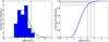 |
Fig. 1 Left: distribution of significances for binary model fits to our calibrators. Right: cumulative distribution of the fitted poisson distribution. We expect no significant asymmetric signal within these stars so use them to form a crude test statistic for our threshold of 4σ. Fitting a poisson distribution we find a confidence level of 88% for a 4σ and more than 95% for 4.5σ. |
Additionally we consider the sample of 54 M-dwarfs observed with SAM as part of an investigation into M dwarf multiplicity by Gaidos et al. (2016) using Keck-II/NIRC2. They found approximately 25% of science targets displayed asymmetric signals within their closure phases in the 4−5σ range. Furthermore, 5% were found to possess signals between 5−6σ. This places lower confidence levels on our 4σ threshold but this sample of targets is likely to be strongly affected by systematics caused by the observation strategy of a single visit and the use of the Laser Guide Star. This will result in little on-sky rotation and inferior calibration so is not as applicable to our data set, except in a cases where we too have little on-sky rotation (i.e. DM Tau). Measured on-sky rotations are displayed in Table A.1.
The fitting procedure outlined above is suitable if the brightness distribution resembles a binary, but it may be inadequate for more complex distributions such as triple systems, or complex disc features. To explore this we create maps of the significances (σ) produced in a binary fit. We use the following equation to produce complex visibilities for theoretical binary models from which we construct model closure phases to fit to our measured closure phases 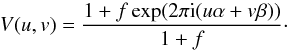 (1)Here, f denotes the flux ratio of the model companion and the parent star, u and v are the Fourier plane coordinates and α and β are the angular coordinates of the companion within the model. We then construct a grid of positions in RA and Dec with a resolution of 1 mas, covering an area of 400 × 400 mas with the parent star located in the centre of the field. At each position we fit for the best contrast and convert the calculated χ2s into a significance to form a map which enables us to make qualitative judgements about whether the detection resembles likely a companion or a more complex brightness distribution. The significance is estimated using:
  (2)where the
  is calculated using Eq. (1) taking an unresolved single point source. We enforce within our fits positive flux and flux ratios less than 1.0, physically representing that the companion cannot be brighter than the parent star.
This modelling approach allows us to search for point source-like asymmetries consistent with a gap-clearing companion. However we are unable to distinguish companions from other potential sources of asymmetry which could mimic a point source in our data sets such as disc over-densities, accretion streams and other complex structure. For this reason we only consider significant detections to be companion candidates in need of further observation rather than confirmed companions. To establish their nature as protoplanets or substellar companions, evidence for orbital motion and ongoing accretion is required.
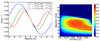 |
Fig. 2 Degeneracy plots of the detection in DM Tau. Left: phases for three companions at three separations and their contrasts according to Eq. (5). Right: fit of the degeneracy profile using the shortest projected baseline length. The fit using the longer baseline well describes the profile at larger separations but poorly describes the shorter separations as the contrast ratio asymptotically goes to 1.0 as the separation approaches λ/2D. The shortest baseline poorly follows the structure at larger separations but does follow closely the profile at closer separations as a result of its ability to probe the more S/N sensitive region close to the λ/2D resolution limit. |
3.2. Degeneracies
Detections of companions with separations ρ ≲ λ/ 2D are problematic to fit because of a degeneracy that appears between the separation and contrast. In this separation regime, the phases do not sample the full sinusoidal modulation that is required to constrain the companion contrast and separation separately. This makes our fits highly sensitive to the signal-to-noise ratio (S/N) of the closure phases, resulting in a range of separations and contrasts that can reproduce the measured non-zero closure phases equally well (see Fig. 2). We therefore find that a similarly good fit can be obtained for different separation/contrast pairings. This is most clearly seen within the significance maps themselves, producing lobe-like structures in the region between λ/D and λ/ 2D.
To explore this degeneracy and allow one to translate from one separation/contrast pair to another we take two approaches. The first approach is to plot the degeneracy directly. We plot a grid of contrasts against separations along the non-degenerate best-fit position angle and construct a significance map in the same manner as outlined above (see Fig. 2). In our second approach, we aim to derive an analytic expression for the separation/contrast degeneracy. For this purpose, we start from Eq. (1) and retrieve the phase component, φ,  (3)where ρ is the scalar companion separation for our best fit position and b is the projected length of the baseline along the vector separation. Rearranging we find:
  (4)For small values of φ (i.e. values of φ<π/ 4) this second equation can be further simplified using the small angle approximation:
  (5)To most accurately trace the profile of the degeneracy, we would need to use every u projected baseline and weight according to their associated uncertainties. However, using simply the shortest projected baseline was found to be effective for tracing the degeneracy to smaller separations. Within our degeneracy plots, the physical degenerate region is shown by the black contour defining the Δσ = 0.5 region, while the white curve displays our analytical solution for the shortest projected baseline (see Fig. 2, right).
In our data set, we find three cases for which the best-fit separation is within the degenerate region. In the case of DM Tau, the uncertainties in our closure phases are small enough to allow us to find a minimum. In this case the degeneracy results in enhanced uncertainties in the separation and contrast measurements. In the remaining cases (FP Tau, K-band; TW Hya, K-band) the S/N for the closure phases prevented our fitting algorithm from finding a minimum χ2. In these cases we set the separation to the resolution limit of our observations; λ/ 2B, where λ is the wavelength of the observations and B is the longest baseline from our mask. However the separations are not well constrained and solutions at larger separations and higher contrasts would result in good fits of similar significances. Our analytical solution enables us to calculate the contrast at a different separation from our fit here.
4. Image reconstruction
In order to retrieve the brightness distribution of the observed objects in a model-independent way, we use image reconstruction techniques developed for infrared long-baseline interferometry on our measured calibrated closure phases and visibilities.
The image estimation from the discrete points in the Fourier plane (the aperture masking measurements) can be considered as an inverse problem. Given that there are more pixels than measurements, the problem is ill-posed and solving it requires one to adopt a Bayesian approach. This amounts to minimising a global cost function (F) defined as:  (6)where Fdata is the likelihood term (here the χ2), Frgl is the regularisation term and μ the regularisation weight (see Thiébaut 2008; Renard et al. 2011, for more background information). The likelihood term ensures that the image is reproducing the data whereas the regularisation term helps to fill the gaps in the Fourier space by interpolating it in a specific way defined by the user. This term helps also to converge to the most likely a-posteriori estimate of the image.
To perform our image reconstructions we have chosen the MiRA algorithm (Thiébaut 2008). This algorithm is minimising the cost function (F) with a downhill gradient method. In our objects the central star is spatially unresolved. In order to image its environment we have therefore modelled it as a point source and reconstruct an image of the environment only, using the approach outlined in Kluska et al. (2014).
The images are defined to have 128 × 128 pixels each. For the pixel size, we chose 5, 7 and 11 mas for H, K and L-bands respectively. We have chosen to use the quadratic smoothness regularisation (Renard et al. 2011). We employed the L-curve method (see Renard et al. 2011; Kluska et al. 2014, for more details) to determine the weight of the regularisation for all data sets and then used the average weight of all the L-curves which is μ = 109.
To define the fraction of the stellar flux in the parametric model, we made a grid of reconstructions with different flux ratios for the star. Because we are minimising the global cost function F we should have chosen the images having the minimum F value. Because of the regularisation effects, these images still have flux at the star position which is not physical. Therefore we decided to keep the flux ratio for which the image has the smaller likelihood term (Fdata). These images do not differ significantly from the images with smaller F except in correcting this effect.
5. Simulations − reference models
Within many of our reconstructed images and significance maps we see patterns or structures which are not consistent with simple point source companions. To aid our understanding of these structures we simulated a range of possible scenarios. We simulate companions with different separations, position angles and contrasts in order to understand potential effects that might be caused by the imperfect uv-coverage and to investigate how the structure of the significance maps changes within the fully resolved and partially resolved regimes described in Sect. 3.2. While we expect these scenarios to cover most structures likely to be seen, this is an incomplete set and other scenarios may occur.
For our simulations we model data sets that correspond to the K-band and the NIRC2 9-hole mask. We add phase noise with a variance of ω = 4°, which resembles good conditions in our observations.
5.1. Small-separation/unresolved companion scenario
In data sets where the companion or disc wall was positioned at separations at or below λ/ 2D we see that the images and significance maps become dominated by the gaussian noise placed in the models (see Fig. 3). In all the cases shown, the artificial companion has a contrast of f = 0.1. We find a much reduced significance compared to a similar companion at larger separations. We therefore consider any companion with a separation below λ/ 2D to be unresolved. In cases where our uv-coverage is sparser caused by the flagging of one or multiple holes during the data reduction process, we often see this noise as periodic signals in the background distribution. The strength of these periodic signals is dependent on the precise uv-coverage and the level of noise in the closure phases.
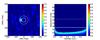 |
Fig. 3 Left: significance map. Right: degeneracy plot. Simulated data of a a companion located at a separation of 10 mas, a position angle of 90°, and contributed 10% of the total flux (white triangle). The white circle shows our best fit position. Within the background it is possible to see noise artefacts caused by holes within the uv-coverage. These holes create periodic signals within the background and may take on geometric patterns. |
Within the reconstructed images, we find that data sets with an unresolved companion will simply be dominated by randomly distributed noise peaks (i.e. TW Hya, K′-band). We also encountered cases, where the image reconstruction algorithm attributed the flux elements of the companion to the central star (e.g. FP Tau, L′-band). Both are shown in Fig. 11. In these cases we are limited to placing lower limits on the possible contrast for a companion around these targets at separations within 200 mas. This limit is set at the 99% confidence level which is determined by the individual noise properties of the data.
5.2. Marginally resolved companion scenario
To study a marginally resolved regime, we simulated data with a companion at a separation of 30 mas. We observe the “strong lobe” structure characteristic of this regime (Fig. 4). In the case of a low-contrast companion (f = 0.1 in the simulation), the degenerate region is reasonably confined, while for higher-contrast companions the “lobes” are large and induce greater errors into estimations of both the position and contrast of any potential companion detection.
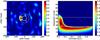 |
Fig. 4 Left: significance map. Right: degeneracy plot. Simulated data of a companion located at a separation of 30 mas, a position angle of 90°, and contributes 10% of the total flux (white triangle). The white circle shows our best fit position. We see the distinctive lobing of a partially resolved companion. In this case with excellent S/N we are able to accurately identify the location of the companion but in practice this is not always the case. |
5.3. Fully-resolved companion scenario
To simulate a fully-resolved companion we computed models with a companion located at a separation of 60 mas, just beyond λ/D. At these separations we can see that the degenerate region has largely disappeared allowing the position of the companion to be well constrained (see Fig. 5).
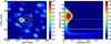 |
Fig. 5 Left: significance map. Right: degeneracy plot. Simulated data for a companion located at a separation of 60 mas, a position angle of 90°, and contributed 10% of the total flux (white triangle). The white circle shows our best fit position. Here the companion is fully resolved and the position and contrast are well constrained. |
5.4. Disc-feature scenario
Asymmetries in the brightness distribution can also be caused by disc-related structures, producing closure phase signals that might be difficult to discern from those produced by close-in companions (Cheetham et al. 2015). To investigate this scenario, we produced synthetic images that are intended to mimic the rim of a disc seen under intermediate inclination (60° from the face-on orientation) with a radius of 30 mas, which corresponds to ~3λ/ 2D. The image shown was produced by simulating a skewed ring with a gaussian profile and a width of 15 mas, a skewness of 0.8, and whose major axis is oriented along position angle 0°. The flux of the disc represents 1% of the total flux in the frame.
Within all the significance maps from this scenario we observe that the significance contours take on double-lobed structures (Fig. 6). This is in agreement with previous work performed by Cheetham et al. (2015), who showed that an inner wall of a optically thick disc will appear as two point-source like structures co-locational with the illuminated rim of the disc, bisected by the center of the disc wall. We find that these also appear within our significance maps and reconstructed images.
Extending the semi-major axis such that the ring appears outside of the degenerate region we begin to resolve the shape of the disc wall. This structure tends to be comparable in strength to the artefacts however and is unseen unless the flux contribution of the disc is not enhanced. This is the result of the flux becoming more spread out within the frame, inducing smaller phase signals.
To make a comparison to a more physical model we create a disc model using the radiative transfer code, TORUS (Harries 2014). Here we can include effects such as forward scattering from the near edge of the disc. We scale this model to have semi-major axes of 30, 45, 60, 90, 120, and 180 mas. The results are shown in Fig. 7. The forward scattered component, while containing more flux, is closer to the central star than the thermal component so only appears at larger separations. It also appears as a single lobe as a resut of flux being most concentrated at the centre of the arc whereas in the thermal case, the flux is more evenly spread across the disc wall. At larger separations this single lobe becomes more resolved, similar to the thermal emission seen in the bottom left frame of Fig. 7 and similarly difficult to distinguish from artefacts.
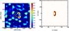 |
Fig. 6 Left: significance map for a simulation with a partially resolved disc wall. The resulting significance maps show two strong detections located at the disc wall. At increasing separations and resolution the two point sources begin to merge. Right: input intensity distribution. Green star indicates the position of the parent star. |
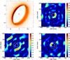 |
Fig. 7 Top left: base model for physical disc simulations. We scale this model for each semi-major axis case. Thermal emission from the far side of the disc is seen in the right side of the frame and forward scattered light in the top left. Top right: 30 mas case. Here we see the double lobe structure caused by the far side of the inner disc wall. Bottom left: 60 mas case. The arc of the far side of the disc wall is clearly seen but is comparable in strength to the artefacts within the frame and so would be difficult to identify in practice. Bottom right: 90 mas case. The forward scattered component is now the dominant feature within the frame. It forms a single lobe owing to the greater concentration of flux in the centre of the arc than in the thermal emission from the opposite side of the disc wall. |
5.5. Disc-asymmetry scenario
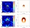 |
Fig. 8 Left: significance map for a simulation with a partially resolved and fully resolved disc asymmetry. The resulting significance maps shows structure similar to a companion detection. Right: input intensity distribution. Green star indicates the position of the parent star. |
To investigate scenarios in which an asymmetry is caused by an over density within the disc we simulate a disc feature with a contrast of 5:1 to the rest of the disc. We take a similar approach to Sect. 5.4 but skew the ring in such a way to resemble possible asymmetries such as those found in simulations by de Val-Borro et al. (2007). These are extreme cases as it is difficult to physically create such a strong contrast particularly in continuum emission (Juhász et al. 2015).
In Fig. 8 we show two cases representing partially resolved and fully resolved cases. Both strongly resemble the structures seen in our companion detection simulations in Sects. 5.2 and 5.3. This should be kept in mind when considering our companion detections without complementary multi-wavelength observations.
Companion candidates.
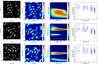 |
Fig. 9 Potential Candidate Detections. Left: reconstructed Image. Middle left: computed significance map. Middle right: degeneracy plot. Right: V2 plots. First row: DM Tau, K-band. Second row: LkHα330, K′-band. Third row: TW Hya, K′-band. |
6. Results
We identify potential candidates through a combination of setting a threshold on the significance of the binary fit and inspection of reconstructed images and significance maps. In Table 3 we list data sets in which we find significant closure phase asymmetries excluding false positives and each case is discussed individually in detail below.
To calculate the semi-major axis for our candidates we assume circular orbits coplanar with the outer disc. Where disc inclination/position angle information is unavailable, we assume a face-on disc. To estimate the companions’ absolute magnitudes, we used the reddening law outlined in Cardelli et al. (1989). From the dereddened absolute magnitudes, we then estimate values of McṀc using the accreting protoplanetary disc models described by Zhu (2015). We match our dereddened absolute magnitudes to the table within Zhu (2015), assuming an inner circumplanetary disc radius of 2 RJ. This is a highly unknown quantity with a significant effect on the resultant values of McṀc. We arbitrarily chose our inner disc radius to be the same value as that assumed by Sallum et al. (2015) for the purposes of comparison. When matching the absolute magntiudes are difficult to match we linearly interpolate. We are unable to directly estimate the mass of a potential companion as these objects are thought to likely possess extended, accreting circumplanetary discs that dominate the infrared excess emission; this prevents us from separating the mass Mc and accretion rate ṀC.
In addition, we place lower limits on the contrast at the 99% confidence level. For the data sets that were recorded under detrimental conditions, our sensitivity is reduced from typical K-band contrasts of Δmλ = 5.5 to values of Δmλ> 5.0.
In the following sections we discuss each object individually. Quoted disc masses represent gas+dust masses and the disc position angles are measured East-of-North along the major axis.
Besides the significance maps derived from closure phase fitting, we also show the visibility amplitudes derived from our observations.
6.1. DM Tau
The structure of the inner 10s of au around DM Tau is complex and difficult to constrain with SED-based models alone. Studying the Spitzer IRS spectrum, Calvet et al. (2005) modelled the SED of DM Tau inferring the presence of a 3 au inner cavity in the disc. In contrast, Andrews et al. (2011) used SMA data to spatially resolve an inner disc cavity with a radius of 19 ± 2 au in 880 μm observations. Neither model however explains simultaneously the IR and sub-mm spectra suggesting the inner disc is potentially populated by a species of small dust grains (Calvet et al. 2005). Andrews et al. (2011) additionally estimated the total disc mass to be 0.04 M⊙ and measured the inclination and position angles of the disc to be 35° and 155° respectively.
The result of our simple binary model indicates a companion at 43 mas (≈6 au) with an absolute magnitude of MK = 11.0 ± 0.3 mag and a significance of 4.27σ (93% confidence level) (see Fig. 9). This places the companion candidate within the disc cavity resolved by Andrews et al. (2011) and outwards of the ring of small dust grains suggested by Calvet et al. (2005). We find a value of McṀc = 10-5  yr-1. The source of the asymmetric signal is located within the partially resolved region nevertheless the S/N in the closure phases is sufficient to constrain the separation through our binary fitting. The net result is an inflation in the uncertainties within the separation and contrast (see Table 3).
We set limits on the contrast of a companion within 200 mas at ΔmK> 4.66 mag and are most sensitive between 40−160 mas where we set lower limits ΔmK> 5.49 mag.
We see a systematic reduction in the visibilities at longer baselines but these remain consistent with an unresolved target.
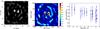 |
Fig. 10 Potential disc feature detections. Left: reconstructed image. Middle: computed significance map. Right: V2 plot. FP Tau, K-band. |
Strong caveats on this detection are placed owing to the small on sky rotation (~1°) and low strength of the detection. The small on-sky rotation in particular makes this case vulnerable to systematics which may mimic a detection. Multiple visits to the target however should aid in reducing such effects but the confidence levels established by comparison to the sample collected by Gaidos et al. (2016) are likely to be more applicable to this case (~ 70%) than the confidence levels established through our sample of calibrators so label this detection as only a possible detection.
6.2. FP Tau
Furlan et al. (2005) classified FP Tau as a Class II object based on Spitzer MIR spectra and inferred the presence of an extended gap within the disc from the lack of NIR excess flux. This was further supported by later analysis by Currie & Sicilia-Aguilar (2011) but neither characterised the spatial extent of the gap. They did however measure the disc mass to be 2.5 × 10⁻⁴ M⊙.
We see clear disc structures within FP Tau, with the K-band data set displaying both “dual lobing” in the significance map and dual point source-like emission in the image (Fig. 10), which we identified in Sect. 5.4 as likely indicators for disc-related asymmetries. From this we conclude the inner edge of the outer disc of FP Tau to be likely moderately inclined and located between 26−52 mas. The S/N of the closure phase is insufficient to find a solution for the separation and we are forced to fix the separation to λ/2D within our fit. This corresponds to ~26 mas and leads to an inner edge located at 10.0 ± 2.0 au where the unknown inclination dominates the uncertainty. Values for the position of the inner rim of the disc can be as large as 20 au however with an equally good fit to the data. Between 50−200 mas we set a lower limit on the contrast of a companion at ΔmK> 5.0 mag.
The L-band data set on FP Tau does not show any significant asymmetries, as can be seen within the significance map. No signal reaches the 4σ significance threshold, which is consistent with the reconstructed images where we see little off-centre flux (see Fig. 11). Between 50−200 mas we set an lower limit on the contrast of a companion as ΔmL> 3.4 mag.
We see a strong drop in the visibilities in the L-band. We fit simple geometric models to the visibilities to estimate the size and orientation of the extended emission. We fit both a ring model and a gaussian profile to the data and find consistent position and inclination angles in both models of 350 ± 20° and 25 ± 5° respectively. We find a semi-major axis of 60 mas in the case of the ring model and a FWHM of 80 mas in the gaussian profile case. We find the K-band visibilities to be consistent with an unresolved object within the measurement uncertainties, indicating a more compact emitting region.
6.3. LkHα 330
LkHα 330 has been extensively studied in unresolved spectroscopy and through interferometry in the millimetre. Brown et al. (2007) inferred a disc gap between 0.7−50 au through SED modelling. This was in agreement with later modelling of the SED by Andrews et al. (2011). They resolved the gap cavity in sub-mm SMA observations, inferring in the process that the infrared emission had its origin within the cleared region gap. They attribute this infrared emission to an additional population of small dust grains located in the gap. The disc was found to have an inclination of 35° and to be oriented along position angle 80°. They estimated the disc mass to be 0.025 M⊙. Isella et al. (2013) carried on further study of the outer disc through the SMA data. They identified a “lopsided” ring in the 1.3 mm thermal dust emission at a radius of 100 au. Through hydrodynamic simulations they find this asymmetric ring to be consistent with perturbations in the surface density of the disc caused by an unseen companion. They set limits on the mass and orbital radius of this companion to >1 MJ and <70 au respectively.
Our observations of LkHα 330 were performed in K- and H-band at two epochs separated by 678 days. We see no significant signal within the H-band data set but do see a strong asymmetric signal within the K-band closure phases indicative of a companion detection.
The contrast of the best-fit companion candidate was found to be ΔmK = 5.5 ± 0.2 mag with a significance level of σ = 4.88. We estimate McṀc to be 10-3 yr-1.
Amongst our companion candidate detections, the K-band observations of LkHα 330 display the most pronounced visibility drop (~0.8−0.9). A strong extended component likely exists around this target, making a considerable contribution to the total flux observed in the K-band. The extended component contributes to the strong periodic patterns seen in the significance maps and reconstructed images (see Fig. 9) caused by holes within our uv-coverage. With the existing data set, we cannot rule out that the aforementioned asymmetric signal may be associated with these artefacts. Additionally our calculated upper limits on the contrast of a companion were found to be ΔmK< 5.5 mag, which are comparable to the contrast of our most significant detection.
Within the H-band observations we do not see the best fit position found in the K-band data set, however to reproduce the observed K-band yr-1 values we would expect contrasts of 6.0−6.2 mag in H-band, well below the 99% confidence level preventing us from ruling out the K-band detections using the H-band observations. We place upper limits on a companion contrast at ΔmH< 4.5 mag.
6.4. RXJ 1615.3-3255
Previous, resolved observations of RXJ 1615.3-3255 are limited. Makarov (2007) linked the object kinematically to the Lupus association at a distance of approximately 185 pc. Henize (1976) and Krautter et al. (1997) classified RXJ 1615.3-3255 as a weak-line T Tauri star, whereas Merín et al. (2010) classified it as a potential transitional disc based on Spitzer spectra.
Andrews et al. (2011) resolved the disc at 880 μm with SMA observations and found that the emission from the disc is highly extended suggesting a large disc extending out to 115 au, and they measure a particularly low-density cavity extending to 30 au. The low density of the cavity forced them to remove all dust from their models from within 0.5 au of the star. The low far-infrared flux of the source was interpreted by them to be as a result of the effects of dust settling in the outer regions of the disc. This leads to a high estimate for the disc mass of 0.13 M⊙, that is ~12% of the stellar mass. They estimated the disc inclination to be 4° with position angle 143°.
We observed RXJ 1615.3-3233 at a single epoch in the K-band and detected a significant asymmetry in the closure phases. However, inspecting the significance maps we see strong similarity between RXJ 1615.3-3233, RXJ 1842.9-3532 and V2062 Oph. All three targets were observed on the same night (09/06/2014) with the same filter and appear to suffer from an systematic effect that results in close to identical structure. The rotation of the structure is equal to the on-sky rotation of the mask. We are not able to identify the precise cause of this systematic effect, but note that the night suffered from poor atmospheric conditions and variable wind speeds, which might have induced vibrations and degraded the AO performance (these poor conditions also reflect in a high variance in the individual uncalibrated closure phase; see Table A.2). The visibilities are also strongly affected by this systematic, showing similar strong drops and structure.
We set a lower limit for the contrast of a potential binary to ΔmK> 4.0 mag between 20−40 mas and ΔmK> 4.6 mag between 40−200 mas (see Fig. 9). The systematics previously mentioned may affect adversely the accuracy of the limits we set in these cases.
6.5. RXJ 1842.9-3532
Hughes et al. (2010) used a combination of resolved SMA observations and SED modelling to infer the presence of an optically thin region inwards from 5 au with a narrow ring of optically thick material at ~0.01−0.2 au. Their models suggest little to no evidence for shadowing from the inner on the outer disc. They estimate the disc mass to be 0.01 M⊙ and measure the inclination to be 54° with a position angle of 32°.
We detect no significant asymmetric signal in the closure phases but see the same systematic structure in the significance maps as in RXJ 1615.3-3255 and V2062 Oph (see Sect. 6.4).
We set lower limits on the contrast of a companion at ΔmK> 5.0 mag between 40−200 mas.
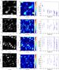 |
Fig. 11 Data sets where we see no significant emission. Left: reconstructed Images. Middle: computed significance maps. Right: V2 plot. First row: FP Tau, L-band. Second row: LkHα330, H-band. Third row: TW Hya, K′-band. Fourth row:, V2246 Oph, K′-band. In these cases we set limits on the contrast of a potential candidate or disc feature. |
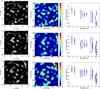 |
Fig. 12 Data sets where we detect significant asymmetric signal but rule it to be a false positive through similarity in structure to other data sets taken during the same night. Left: reconstructed Images Middle: computed significance maps. Right: V2 plots. First row: RXJ 1615.3-3255, K-band, Second row: RXJ 1842.9-3532, K-band, Third row: V2062 Oph, K′-band. We rule out these asymmetries because of the similarity in the structure of their artefacts. All three targets were observed on the same night and the same structure is also observed in some of the calibrators. The position angle of the structures differ by the same angle as the on sky rotation of the 9-hole mask (See Sects. 6.5 and 6.7). The cause of this effect is unknown. |
6.6. TW Hya
Estimates by Calvet et al. (2002) found that the optically-thick disc of TW Hya extends from 4 to 140 au, with a mass of 0.06 M⊙ for a 10 Myr old disc. They additionally found that the inner region of the disc is not fully cleared. A population of 1 μm dust grains is required within the optically thin inner 4 au to properly fit the SED in agreement with observed continued accretion onto TW Hya. This interpretation is supported by recent ALMA observations by Andrews et al. (2016) which probed, through 870 μm emission, the distribution of millimeter-sized grains to spatial scales on the order of an au. They observed ring structures suggestive of ongoing planet formation, in particular an unresolved inner disc within 0.5 au and a bright ring at 2.4 au separated by a dark annulus centred at 1 au.
Radial velocity studies of this object performed by Setiawan et al. (2008) provided evidence for the presence of a 9.8 ± 3.3 MJ planet on an orbit with a semi-major axis of 0.041 ± 0.002 au. This body could be responsible for the clearing of the inner regions of the disc. This interpretation of the RV data was disputed by Huélamo et al. (2008), who attributed the signal to the presence of a cool stellar spot.
TW Hya was also observed as part of the AO imaging survey with Keck II by Brandeker et al. (2003). They detected no companion in the H-band down to contrasts of ~1 mag at 0 05, increasing approximately linearly to 4 mag at 02, corresponding to distances of 2.75 to 11 au.
Using VLT/NACO, Vicente et al. (2011) searched for a potential companion in 1.75 μm and 2.12 μm. They employed the LOCI PSF removal algorithm and detected no companion more massive than 0.11 M⊙ outward of 5.5 au (01) or brown dwarf companion outward of 7 au (013) or planetary mass outward of 13 au (024) at a contrast of 2 mag. Outward of 87 au they achieve their maximum contrast sensitivity of 8 mag allowing them to rule out companions above 7 MJ. Evans et al. (2012) observed TW Hya with Keck-II/CONICA in L-band in March, 2009 and observed no significant asymmetric signal within 200 mas and set lower limits on the contrast of a companion.
We observed TW Hya twice in the K-band on non-consecutive nights in the same epoch. In the data from the first night, we see a significant asymmetric signal corresponding to a contrast of ΔmK = 5.6 ± 0.3 mag (see Fig. 9). Assuming that the potential companion orbits co-planar to the disc, we find a corresponding semi major axis of ~6 au with  yr-1. We set limits on the contrast of a companion at ΔmK > 5.4 mag between 20−200 mas. We additionally see no significant drop in the visibilities.
On the second night we see no significant asymmetries. The poor atmospheric conditions lead to large uncertainties in the closure phases as a result of frequent loss of AO lock during observation. The result can be seen in the significance map and in particular the reconstructed image where strong bands of artefacts are visible (see Fig. 11). The contrast limits from the second night are also adversely affected. Between 80−160 mas we set contrast limits of ΔmK > 3.5 mag, preventing us from ruling out the detection from the first night.
Comparing our result from the first night to the limits in L-band set by Evans et al. (2012), we use the circumplanetary disc models in Zhu (2015) to estimate the L-band absolute magnitude an accreting companion of this absolute magnitude would display. We find the expected contrast to be ΔmL ≈ 4 mag compared to the limit imposed by Evans et al. (2012) of ΔmL > 6 mag. Assuming the scaling described within the circumplanetary disc models to be accurate, to account for both observations the accretion rate onto the potential companion would be required to increase by at least an order of magnitude during the three years separating the observations. The value of Ṁ onto TW Hya is known to be highly variable with values fluctuating at least by an order of magnitude (Alencar & Batalha 2002). This variation occurs on a time scale of years and we would expect the accretion rate onto a companion to be related to the amount of material flowing through the disc so we cannot rule out this companion candidate based on previous SAM observations.
Another possible cause is that the origin of this asymmetry is not protoplanetary in nature but instead from a another potential source of asymmetry such as an accretion stream or disc asymmetry. ALMA observations carried out by Andrews et al. (2016) at ~350 GHz found no non-axisymmetric structures on these scales within the distribution of sub-mm particles but this does not rule out a disc asymmetry in our data set as our K-band observations probe the surface layer of the disc while their sub-mm observations probe the middle of the disc (Juhász et al. 2015). We lack the required signal to noise to be sensitive to any companion within the 1 au gap seen in their sub-mm data but find no significant asymmetry in the bright ring at 2.4 au. We additionally note that if confirmed, our companion candidate would lie immediately outside the bright ring seen in the sub-mm data where the intensity distribution flattens out at ~6 au. ALMA observations taken in 138 and 230 GHz (Tsukagoshi et al. 2016) revealed a shallow gap of a few percent centred at ~6 au in agreement with the location of our companion candidate.
6.7. V2062 Oph
Espaillat et al. (2010) modelled the Spitzer SED and found a disc cavity extending to 36 au containing some optically thin dust consistent with other resolved observations of V2062 Oph. Andrews et al. (2011) finds a cavity in the disc extending out to 30 au. They additionally constrained the inclination and position angle to 35° and 80° respectively and they estimate the disc mass to be 0.007 M⊙.
We observed V2062 Oph in the K-band within a single epoch. Observing conditions were not ideal, but we detect a significant asymmetry signal in the closure phases. As mentioned previously in Sect. 6.4, the produced structures are also reproduced within the RXJ 1615.3-3255 and RXJ 1842.9-3532 data sets leading to the conclusion that these are false positives along with V2062 Oph.
We set lower limits on the contrast of a companion at ΔmK > 4.9 mag between 20−40 mas and >5.1 mag between 40−200 mas.
6.8. V2246 Oph
Mid-infrared 9−18 μm Gemini observations by Jensen et al. (2009) resolved V2246 Oph at subarcsecond resolution and found very little MIR excess within 100 au. Beyond this region they observed strongly extended and asymmetric emission out to 100s of au. The asymmetric emission forms a half ring structure to the north west, at an angular separation of  .
.
Vicente et al. (2011) observed V2246 Oph as part of their VLT/NACO high resolution observations. They reached sensitivities of 15 MJ and 6 MJ past separations of 3 au and 192 au respectively. They found no evidence for a companion within these limits.
We observed V2246 Oph in the K-band in a single epoch. Poor observing conditions severely limited the sensitivity of our observations. We place limits on the contrast of a potential companion at ΔmK > 2.3 mag between 20−40 mas and >3.1 mag between 40-200 mas.
7. Conclusions
In this paper we presented results of five nights of Keck sparse aperture masking observations on eight targets in K-band, one in L-band (FP Tau), one in H-band (LkHα 330). Within this data set we find significant non-zero closure phases for six targets, indicating asymmetries in the brightness distribution on scales of few au. We however rule three of these to be false positives caused by a systematic effect that affected one of our observing nights. The remaining detected asymmetries indicate either the presence of complex disc structures and/or the presence of companions. We conducted detailed simulations in order to understand the signature that these different scenarios produce in our phase measurements and investigated the degeneracies that occur between the derived separation and contrast parameters in the case of marginally resolved companions.
Using both modelling and image reconstruction methods, we investigated the likely origin of the asymmetries for each target star. We estimate confidence levels for our companion detections through fitting companion models to a sample of 24 calibrators stars known to be point source-like. We use the resultant ditribution to form our confidence levels. We report companion detections at a confidence level of >99% (>4.5σ) in LkHα 330 and detections in two further stars (TW Hya and DM Tau) at the lower confidence level of >95% (>4.0σ). For the detections, we derive McṀc values of 10-3 yr-1 (LkHα330), 10-5 yr-1 (DM Tau) and, 10-5 yr-1 (TW Hya). Additionally we infer through comparison to limits previously set on the contrast of a companion in L-band that the origin of the asymmetry signal within the TW Hya data set would require an increase in the accretion rate of an order of magnitude within a few years for it to be consistent with an accreting protoplanet, assuming accurate scaling from L- to K-band. Observations by Alencar & Batalha (2002) indicate TW Hya to be a highly variable disc with values of Ṁ varying by an order of magnitude over time scales of a year, adding support to this scenario.
In LkHα 330 and DM Tau the gap properties have been characterised by earlier observations and we find the companion candidates to be located within the disc gaps, suggesting that they are orbiting within the cleared regions of the disc. In the case of TW Hya we find the companion candidate to be located on the outer edge of the bright annulus located at 2.4 au in recent 350 GHz ALMA observations by Andrews et al. (2016). Furthermore we find that separation of our companion candidate to lie within the shallow gap at 6 au observed by Tsukagoshi et al. (2016) in 138 and 230 GHz ALMA observations.
We interpret the asymmetries in FP Tau be associated with disc emission, most likely a disc wall between 20−40 mas, similar to the asymmetries seen in T Cha (Cheetham et al. 2015) and FL Cha (Cieza et al. 2013). This is supported through strong drops in the visibilties in both the K- and L-band observations of this target. Fitting geometric disc models to the data sets we find find visibilities consistent with a compact emitting region in K-Band and an extended component in L-band with a position angle of 350 ± 20° and an inclination of 25 ± 5°. Finally, for the remaining data sets we detect no significant asymmetries and set lower limits on the contrast of potential companions.
With the detection of significant asymmetries in four out of eight target stars, our detection frequency is relatively high (50%). This is higher than the detection rate that was found in surveys of other object classes (14%: Kraus et al. 2008; 20%: Kraus et al. 2011) conducted with Keck/NIRC2 SAM interferometry with a same observational setup and a similar data analysis scheme. This demonstrates that transitional discs indeed trace a particularly interesting phase in disc evolution and highlights the need for further studies on these object classes with the unique observational window that SAM provides, both with the current-generation telescopes and the upcoming generation of Extremely Large Telescopes. Besides further continuum imaging, it is promising to image these objects in accretion tracing spectral lines such as Hα, in order to confirm that these objects are sites of continued accretion and to ultimately establish their classification as protoplanets.
Acknowledgments
We acknowledge support from a STFC Rutherford Fellowship and Grant (ST/J004030/1, ST/K003445/1), Marie Sklodowska-Curie CIG grant (Ref. 618910), and Philip Leverhulme Prize (PLP-2013-110). We additionally acknowledge support from NASA KPDA grants (JPL-1452321, 1474717, 1485953, 1496788). The authors wish to recognise and acknowledge the very significant cultural role and reverence that the summit of Mauna Kea has always had within the indigenous Hawaiian community. We are most fortunate to have the opportunity to conduct observations from this mountain. Some of the data presented herein were obtained at the W.M. Keck Observatory, which is operated as a scientific partnership among the California Institute of Technology, the University of California and the National Aeronautics and Space Administration. The Observatory was made possible by the generous financial support of the W.M. Keck Foundation.
References
- Alencar, S. H. P., & Batalha, C. 2002, ApJ, 571, 378 [NASA ADS] [CrossRef] [Google Scholar]
- Alencar, S. H. P., Teixeira, P. S., Guimarães, M. M., et al. 2010, A&A, 519, A88 [NASA ADS] [CrossRef] [EDP Sciences] [Google Scholar]
- Andrews, S. M., Wilner, D. J., Espaillat, C., et al. 2011, ApJ, 732, 42 [NASA ADS] [CrossRef] [Google Scholar]
- Andrews, S. M., Wilner, D. J., Zhu, Z., et al. 2016, ApJ, 820, L40 [NASA ADS] [CrossRef] [Google Scholar]
- Armitage, P. J. 2011, ARA&A, 49, 195 [NASA ADS] [CrossRef] [EDP Sciences] [Google Scholar]
- Ayliffe, B. A., & Bate, M. R. 2012, MNRAS, 427, 2597 [NASA ADS] [CrossRef] [Google Scholar]
- Biller, B., Lacour, S., Juhász, A., et al. 2012, ApJ, 753, L38 [NASA ADS] [CrossRef] [Google Scholar]
- Birnstiel, T., Ormel, C. W., & Dullemond, C. P. 2011, A&A, 525, A11 [NASA ADS] [CrossRef] [EDP Sciences] [Google Scholar]
- Bouvier, J., & Appenzeller, I. 1992, A&AS, 92, 481 [Google Scholar]
- Bouvier, J., Alencar, S. H. P., Boutelier, T., et al. 2007, A&A, 463, 1017 [NASA ADS] [CrossRef] [EDP Sciences] [Google Scholar]
- Brandeker, A., Jayawardhana, R., & Najita, J. 2003, AJ, 126, 2009 [NASA ADS] [CrossRef] [Google Scholar]
- Brauer, F., Dullemond, C. P., & Henning, T. 2008, A&A, 480, 859 [NASA ADS] [CrossRef] [EDP Sciences] [Google Scholar]
- Brown, J. M., Blake, G. A., Dullemond, C. P., et al. 2007, ApJ, 664, L107 [NASA ADS] [CrossRef] [Google Scholar]
- Brown, J. M., Blake, G. A., Qi, C., et al. 2009, ApJ, 704, 496 [NASA ADS] [CrossRef] [Google Scholar]
- Calvet, N., D’Alessio, P., Hartmann, L., et al. 2002, ApJ, 568, 1008 [NASA ADS] [CrossRef] [Google Scholar]
- Calvet, N., Muzerolle, J., Briceño, C., et al. 2004, AJ, 128, 1294 [NASA ADS] [CrossRef] [Google Scholar]
- Calvet, N., D’Alessio, P., Watson, D. M., et al. 2005, ApJ, 630, L185 [NASA ADS] [CrossRef] [Google Scholar]
- Cardelli, J. A., Clayton, G. C., & Mathis, J. S. 1989, ApJ, 345, 245 [NASA ADS] [CrossRef] [Google Scholar]
- Cheetham, A., Huélamo, N., Lacour, S., de Gregorio-Monsalvo, I., & Tuthill, P. 2015, MNRAS, 450, L1 [NASA ADS] [CrossRef] [Google Scholar]
- Chen, H., Myers, P. C., Ladd, E. F., & Wood, D. O. S. 1995, ApJ, 445, 377 [NASA ADS] [CrossRef] [Google Scholar]
- Cieza, L. A., Lacour, S., Schreiber, M. R., et al. 2013, ApJ, 762, L12 [NASA ADS] [CrossRef] [Google Scholar]
- Currie, T., & Sicilia-Aguilar, A. 2011, ApJ, 732, 24 [NASA ADS] [CrossRef] [Google Scholar]
- de Val-Borro, M., Artymowicz, P., D’Angelo, G., & Peplinski, A. 2007, A&A, 471, 1043 [NASA ADS] [CrossRef] [EDP Sciences] [Google Scholar]
- Espaillat, C., D’Alessio, P., Hernández, J., et al. 2010, ApJ, 717, 441 [NASA ADS] [CrossRef] [Google Scholar]
- Espaillat, C., Furlan, E., D’Alessio, P., et al. 2011, ApJ, 728, 49 [NASA ADS] [CrossRef] [Google Scholar]
- Espaillat, C., Muzerolle, J., Najita, J., et al. 2014, Protostars and Planets VI, 497 [Google Scholar]
- Evans, T. M., Ireland, M. J., Kraus, A. L., et al. 2012, ApJ, 744, 120 [NASA ADS] [CrossRef] [Google Scholar]
- Fernandez, M., Ortiz, E., Eiroa, C., & Miranda, L. F. 1995, A&AS, 114, 439 [NASA ADS] [Google Scholar]
- Fouchet, L., Gonzalez, J.-F., & Maddison, S. T. 2010, A&A, 518, A16 [NASA ADS] [CrossRef] [EDP Sciences] [Google Scholar]
- Furlan, E., Calvet, N., D’Alessio, P., et al. 2005, ApJ, 628, L65 [NASA ADS] [CrossRef] [Google Scholar]
- Furlan, E., Hartmann, L., Calvet, N., et al. 2006, ApJS, 165, 568 [NASA ADS] [CrossRef] [MathSciNet] [Google Scholar]
- Gaidos, E., Mann, A. W., Kraus, A. L., & Ireland, M. 2016, MNRAS, 457, 2877 [NASA ADS] [CrossRef] [Google Scholar]
- Grady, C. A., Muto, T., Hashimoto, J., et al. 2013, ApJ, 762, 48 [NASA ADS] [CrossRef] [Google Scholar]
- Harries, T. 2014, TORUS: Radiation transport and hydrodynamics code [record ascl:1404.006] [Google Scholar]
- Hashimoto, J., Tamura, M., Muto, T., et al. 2011, ApJ, 729, L17 [NASA ADS] [CrossRef] [Google Scholar]
- Henize, K. G. 1976, ApJS, 30, 491 [NASA ADS] [CrossRef] [Google Scholar]
- Huélamo, N., Figueira, P., Bonfils, X., et al. 2008, A&A, 489, L9 [NASA ADS] [CrossRef] [EDP Sciences] [Google Scholar]
- Huélamo, N., Lacour, S., Tuthill, P., et al. 2011, A&A, 528, L7 [NASA ADS] [CrossRef] [EDP Sciences] [Google Scholar]
- Hughes, A. M., Andrews, S. M., Wilner, D. J., et al. 2010, AJ, 140, 887 [NASA ADS] [CrossRef] [Google Scholar]
- Ireland, M. J., & Kraus, A. L. 2008, ApJ, 678, L59 [NASA ADS] [CrossRef] [Google Scholar]
- Isella, A., Pérez, L. M., Carpenter, J. M., et al. 2013, ApJ, 775, 30 [NASA ADS] [CrossRef] [MathSciNet] [Google Scholar]
- Jensen, E. L. N., Cohen, D. H., & Gagné, M. 2009, ApJ, 703, 252 [NASA ADS] [CrossRef] [Google Scholar]
- Juhász, A., Benisty, M., Pohl, A., et al. 2015, MNRAS, 451, 1147 [NASA ADS] [CrossRef] [Google Scholar]
- Kenyon, S. J., Brown, D. I., Tout, C. A., & Berlind, P. 1998, AJ, 115, 2491 [NASA ADS] [CrossRef] [Google Scholar]
- Kluska, J., Malbet, F., Berger, J.-P., et al. 2014, A&A, 564, A80 [NASA ADS] [CrossRef] [EDP Sciences] [Google Scholar]
- Kraus, A. L., & Ireland, M. J. 2012, ApJ, 745, 5 [NASA ADS] [CrossRef] [Google Scholar]
- Kraus, A. L., Ireland, M. J., Martinache, F., & Lloyd, J. P. 2008, ApJ, 679, 762 [NASA ADS] [CrossRef] [Google Scholar]
- Kraus, A. L., Ireland, M. J., Martinache, F., & Hillenbrand, L. A. 2011, ApJ, 731, 8 [NASA ADS] [CrossRef] [Google Scholar]
- Kraus, S., Ireland, M. J., Sitko, M. L., et al. 2013, ApJ, 768, 80 [NASA ADS] [CrossRef] [Google Scholar]
- Krautter, J., Wichmann, R., Schmitt, J. H. M. M., et al. 1997, A&AS, 123, 329 [NASA ADS] [CrossRef] [EDP Sciences] [Google Scholar]
- Loinard, L., Torres, R. M., Mioduszewski, A. J., & Rodríguez, L. F. 2008, ApJ, 675, L29 [NASA ADS] [CrossRef] [Google Scholar]
- Makarov, V. V. 2007, ApJ, 658, 480 [NASA ADS] [CrossRef] [Google Scholar]
- Merín, B., Brown, J. M., Oliveira, I., et al. 2010, ApJ, 718, 1200 [NASA ADS] [CrossRef] [Google Scholar]
- Muzerolle, J., Flaherty, K., Balog, Z., et al. 2009, ApJ, 704, L15 [NASA ADS] [CrossRef] [Google Scholar]
- Najita, J. R., Strom, S. E., & Muzerolle, J. 2007, MNRAS, 378, 369 [NASA ADS] [CrossRef] [Google Scholar]
- Olofsson, J., Benisty, M., Le Bouquin, J.-B., et al. 2013, A&A, 552, A4 [NASA ADS] [CrossRef] [EDP Sciences] [Google Scholar]
- Pollack, J. B., Hubickyj, O., Bodenheimer, P., et al. 1996, Icarus, 124, 62 [NASA ADS] [CrossRef] [Google Scholar]
- Reipurth, B., Pedrosa, A., & Lago, M. T. V. T. 1996, A&AS, 120, 229 [NASA ADS] [CrossRef] [EDP Sciences] [Google Scholar]
- Renard, S., Thiébaut, E., & Malbet, F. 2011, A&A, 533, A64 [NASA ADS] [CrossRef] [EDP Sciences] [Google Scholar]
- Sallum, S., Follette, K. B., Eisner, J. A., et al. 2015, Nature, 527, 342 [NASA ADS] [CrossRef] [Google Scholar]
- Setiawan, J., Henning, T., Launhardt, R., et al. 2008, Nature, 451, 38 [NASA ADS] [CrossRef] [PubMed] [Google Scholar]
- Silverstone, M. D., Meyer, M. R., Mamajek, E. E., et al. 2006, ApJ, 639, 1138 [NASA ADS] [CrossRef] [Google Scholar]
- Thiébaut, E. 2008, in SPIE Conf. Ser., 7013, 1 [Google Scholar]
- Tsukagoshi, T., Nomura, H., Muto, T., et al. 2016, ApJ, 829, L35 [NASA ADS] [CrossRef] [Google Scholar]
- Varnière, P., Blackman, E. G., Frank, A., & Quillen, A. C. 2006, ApJ, 640, 1110 [NASA ADS] [CrossRef] [Google Scholar]
- Vicente, S., Merín, B., Hartung, M., et al. 2011, A&A, 533, A135 [NASA ADS] [CrossRef] [EDP Sciences] [Google Scholar]
- White, R. J., Gabor, J. M., & Hillenbrand, L. A. 2007, AJ, 133, 2524 [NASA ADS] [CrossRef] [Google Scholar]
- Zhu, Z. 2015, ApJ, 799, 16 [NASA ADS] [CrossRef] [Google Scholar]
Appendix A: Additional tables
Log for our Keck/NIRC2 observations.
Phase noise variance ω for uncalibrated closures phases.
All Tables
All Figures
|
Fig. 1 Left: distribution of significances for binary model fits to our calibrators. Right: cumulative distribution of the fitted poisson distribution. We expect no significant asymmetric signal within these stars so use them to form a crude test statistic for our threshold of 4σ. Fitting a poisson distribution we find a confidence level of 88% for a 4σ and more than 95% for 4.5σ. |
| In the text | |
|
Fig. 2 Degeneracy plots of the detection in DM Tau. Left: phases for three companions at three separations and their contrasts according to Eq. (5). Right: fit of the degeneracy profile using the shortest projected baseline length. The fit using the longer baseline well describes the profile at larger separations but poorly describes the shorter separations as the contrast ratio asymptotically goes to 1.0 as the separation approaches λ/2D. The shortest baseline poorly follows the structure at larger separations but does follow closely the profile at closer separations as a result of its ability to probe the more S/N sensitive region close to the λ/2D resolution limit. |
| In the text | |
|
Fig. 3 Left: significance map. Right: degeneracy plot. Simulated data of a a companion located at a separation of 10 mas, a position angle of 90°, and contributed 10% of the total flux (white triangle). The white circle shows our best fit position. Within the background it is possible to see noise artefacts caused by holes within the uv-coverage. These holes create periodic signals within the background and may take on geometric patterns. |
| In the text | |
|
Fig. 4 Left: significance map. Right: degeneracy plot. Simulated data of a companion located at a separation of 30 mas, a position angle of 90°, and contributes 10% of the total flux (white triangle). The white circle shows our best fit position. We see the distinctive lobing of a partially resolved companion. In this case with excellent S/N we are able to accurately identify the location of the companion but in practice this is not always the case. |
| In the text | |
|
Fig. 5 Left: significance map. Right: degeneracy plot. Simulated data for a companion located at a separation of 60 mas, a position angle of 90°, and contributed 10% of the total flux (white triangle). The white circle shows our best fit position. Here the companion is fully resolved and the position and contrast are well constrained. |
| In the text | |
|
Fig. 6 Left: significance map for a simulation with a partially resolved disc wall. The resulting significance maps show two strong detections located at the disc wall. At increasing separations and resolution the two point sources begin to merge. Right: input intensity distribution. Green star indicates the position of the parent star. |
| In the text | |
|
Fig. 7 Top left: base model for physical disc simulations. We scale this model for each semi-major axis case. Thermal emission from the far side of the disc is seen in the right side of the frame and forward scattered light in the top left. Top right: 30 mas case. Here we see the double lobe structure caused by the far side of the inner disc wall. Bottom left: 60 mas case. The arc of the far side of the disc wall is clearly seen but is comparable in strength to the artefacts within the frame and so would be difficult to identify in practice. Bottom right: 90 mas case. The forward scattered component is now the dominant feature within the frame. It forms a single lobe owing to the greater concentration of flux in the centre of the arc than in the thermal emission from the opposite side of the disc wall. |
| In the text | |
|
Fig. 8 Left: significance map for a simulation with a partially resolved and fully resolved disc asymmetry. The resulting significance maps shows structure similar to a companion detection. Right: input intensity distribution. Green star indicates the position of the parent star. |
| In the text | |
|
Fig. 9 Potential Candidate Detections. Left: reconstructed Image. Middle left: computed significance map. Middle right: degeneracy plot. Right: V2 plots. First row: DM Tau, K-band. Second row: LkHα330, K′-band. Third row: TW Hya, K′-band. |
| In the text | |
|
Fig. 10 Potential disc feature detections. Left: reconstructed image. Middle: computed significance map. Right: V2 plot. FP Tau, K-band. |
| In the text | |
|
Fig. 11 Data sets where we see no significant emission. Left: reconstructed Images. Middle: computed significance maps. Right: V2 plot. First row: FP Tau, L-band. Second row: LkHα330, H-band. Third row: TW Hya, K′-band. Fourth row:, V2246 Oph, K′-band. In these cases we set limits on the contrast of a potential candidate or disc feature. |
| In the text | |
|
Fig. 12 Data sets where we detect significant asymmetric signal but rule it to be a false positive through similarity in structure to other data sets taken during the same night. Left: reconstructed Images Middle: computed significance maps. Right: V2 plots. First row: RXJ 1615.3-3255, K-band, Second row: RXJ 1842.9-3532, K-band, Third row: V2062 Oph, K′-band. We rule out these asymmetries because of the similarity in the structure of their artefacts. All three targets were observed on the same night and the same structure is also observed in some of the calibrators. The position angle of the structures differ by the same angle as the on sky rotation of the 9-hole mask (See Sects. 6.5 and 6.7). The cause of this effect is unknown. |
| In the text | |
Current usage metrics show cumulative count of Article Views (full-text article views including HTML views, PDF and ePub downloads, according to the available data) and Abstracts Views on Vision4Press platform.
Data correspond to usage on the plateform after 2015. The current usage metrics is available 48-96 hours after online publication and is updated daily on week days.
Initial download of the metrics may take a while.