| Issue |
A&A
Volume 595, November 2016
|
|
|---|---|---|
| Article Number | A76 | |
| Number of page(s) | 17 | |
| Section | Interstellar and circumstellar matter | |
| DOI | https://doi.org/10.1051/0004-6361/201628853 | |
| Published online | 01 November 2016 | |
The small-scale HH34 IRS jet as seen by X-shooter⋆
1 INAF–Osservatorio Astronomico di Roma, via di Frascati 33, 00078 Monte Porzio Catone, Italy
e-mail: This email address is being protected from spambots. You need JavaScript enabled to view it.
2 INAF–Osservatorio Astronomico di Capodimonte, via Moiariello, 16, 80131 Napoli, Italy
3 INAF–Osservatorio Astrofisico di Arcetri, Largo E. Fermi 5, 50125 Firenze, Italy
Received: 4 May 2016
Accepted: 14 July 2016
Abstract
Context. Atomic jets are a common phenomenon among young stars, being intimately related to disk accretion. Most studies have been performed on jets from pre-main sequence stars. However, to date very little detailed information has been gathered on jets from young embedded low mass sources (the so-called class I stars), especially in the inner jet region.
Aims. We exploit a diagnostic analysis based on multiwave spectroscopic observations to infer kinematics and physical conditions of the inner region of the prototypical class I jet from HH34 IRS.
Methods. We use a deep X-shooter spectrum covering the wavelength range 350−2300 nm at resolution between ~8000 and ~18 000 (i.e., ΔV ~ 17−27 km s-1), which allows us to detect lines in a wide range of excitation conditions (from Eup ~ 8000 to ~31 000 cm-1 ) and to study their kinematics. Statistical equilibrium and ionization models are adopted to derive the jet main physical parameters.
Results. We separately derive the physical conditions for the extended high velocity jet (HVC, Vr ~−100 km s-1 ) and for the low velocity and compact gas (LVC, Vr ~ −20−50 km s-1) located on-source. Close to the jet base (<200 AU from source) the HVC gas is mostly neutral (xe < 0.1) and very dense (nH > 5 × 105 cm-3). The LVC gas has the same density and AV as the HVC, but it is at least a factor of two colder. Iron abundance in the HVC is consistent with the solar value, while it is a factor of 3 subsolar in the LVC, suggesting an origin of the LVC gas from a dusty disk. From the derived total density we infer that the jet mass flux rate is >5 × 10⁻⁷M⊙ yr-1. We find that the relationships between accretion luminosity and permitted line luminosity derived for T Tauri stars cannot be directly extended to class I sources embedded in reflection nebulae since the permitted lines are seen through scattered light. An accretion rate of ~7 × 10⁻⁶M⊙ yr-1 is instead derived from an empirical relationship connecting Ṁacc with L([O i])(HVC).
Conclusions. The class I HH34 IRS jet at small scale shares many kinematical and physical properties with the jets from the most active classical T Tauri (CTT) stars. However, the HH34 IRS jet is denser as a consequence of the larger mass ejection rate with respect to typical values in CTTs jets. These findings suggests that the acceleration and excitation mechanisms in collimated jets are not influenced by evolution and are similar in CTTs and in still embedded sources with high accretion rates.
Key words: stars: formation / stars: protostars / ISM: jets and outflows / ISM: individual objects: HH34
Based on Observations collected with X-shooter at the Very Large Telescope on Cerro Paranal (Chile), operated by the European Southern Observatory (ESO). Program ID: 090.C-0606.
© ESO, 2016
1. Introduction
High velocity outflows from young stellar objects (YSOs) are intimately related to the accretion process of star formation. It has been suggested that outflows from accreting YSOs have a fundamental role in removing angular momentum from circumstellar disk material allowing infalling matter to accrete onto the central star. Hence, determining the nature of the mechanism responsible for the formation of jets in young stars is critical in order to understand the underlying accretion. The details of this coupled accretion-ejection mechanism are still poorly understood, although magnetic fields almost certainly play a central role in this process. Whether originating from the stellar object, from the inner disk edge, from a large section of the accreting disk, or from a combination of the above (e.g., Ferreira et al. 2006; Shang et al. 2007), the jet launching region is predicted to be located at fractions of AU from the central source, thus preventing a direct observational view with current optical/near-infrared telescope technology. However, constraints on the jet launching mechanism can be inferred from observations of the outflows within a few arcsec of the central star where the jet is expected to be still largely unaffected by ambient gas. In particular, significant effort has been devoted to inferring kinematic and excitation conditions in these small-scale micro-jets from classical T Tauri (CTT) stars, where the original circumstellar envelope has already been cleared out and the star–disk interaction region is exposed to a direct observational view (see, e.g., Ray et al. 2007; Frank et al. 2014, and references therein).
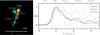 |
Fig. 1 Left: adopted X-shooter slit over a [Fe II] 1.64 μm narrow band image of the HH34 jet obtained with LBT-LUCI (Antoniucci et al. 2014a). The blue circle indicates the source position at α = 05h35m29 |

Investigation of jets from younger and more embedded objects (the so-called class I objects) is more challenging, however, owing to the high extinction close to the source that limits a direct view of the jet base. In class I sources, the jet base has been studied mainly in the IR as these micro-jets are particularly bright in [Fe ii] forbidden and H2 ro-vibrational emission lines (Davis et al. 2003, 2011; Garcia Lopez et al. 2008; 2010). Observations of [Fe ii] lines indicate that within the first 300 AU, class I jets have a kinematical behavior similar to the atomic jets of CTT stars. They share, in particular, a similar forbidden emission line (FEL) region consisting of a high velocity extended component (HVC) and a compact component close to systemic velocity (LVC; e.g., Hartigan et al. 1995; Davis et al. 2003; Takami et al. 2006). However, although [Fe ii] IR line ratios are used to measure the jet electron density, no stringent constraints on the full set of physical parameters, including temperature and ionization fraction, can be derived with only the IR lines. This has limited a more quantitative assessment about the influence of evolutionary effects on the physical and dynamical properties of the class I micro-jets.
In order to address the above issue, we report here deep observations of the class I source HH34 IRS obtained with the X-shooter instrument on VLT (Vernet et al. 2011). The X-shooter simultaneously covers the spectral range between 0.3 to 2.4 μm with a spectral resolution high enough (up to ~17 km s-1) to resolve the main jet kinematical components. Such observations can therefore be very effective in probing the excitation structure of the jet at small scale using a wide range of diagnostic lines (Bacciotti et al. 2011; Ellerbroek et al. 2013; Giannini et al. 2013; Whelan et al. 2014).
HH34 IRS is an embedded low-mass object (M∗ ~ 0.5 M⊙, L∗ ~ 15 L⊙, Antoniucci et al. 2008) located in the L1642 cloud (d = 414 pc) and driving the well-known HH34 parsec scale flow. The flow and its associated HH objects are driven by a collimated blue-shifted jet, which extends for about 30′′ and is bright both in optical and IR images (e.g., Reipurth et al. 2002; Antoniucci et al. 2014a). This makes HH34 an ideal target to exploit the X-shooter multiwavelength capabilities.
High resolution optical imaging and spectroscopy have mainly been used to study the morphology and kinematics of the jet (e.g., Reipurth et al. 2002; Beck et al. 2007; Raga et al. 2012). Multi-epoch HST observations have indicated that the jet is subject to variations in velocity and jet axis direction, which can be due to precession of the outflow source around a possible companion. Infrared spectroscopy has revealed for the first time the presence of a counter-jet (Garcia Lopez et al. 2008), later imaged with Spitzer (Raga et al. 2011). Several spectroscopic studies in the infrared have been conducted on the HH34 jet, showing that it emits copiously in both [Fe ii] and H2 transitions (Takami et al. 2006; Garcia Lopez et al. 2008; Davis et al. 2011). An analysis combining both IR and optical spectroscopy has been applied by Podio et al. (2006) to infer the jet excitation structure at large scale.
Taking advantage of the higher sensitivity, resolution, and spectral coverage of the X-shooter, we can now derive better estimates on the physical conditions at the base of the HH34 micro-jet and investigate the relationship between gas excitation and kinematics. This information can be used to constrain the mechanism responsible for the jet formation and to discuss the similarities and differences with jets in CTT stars.
The paper is structured as follows. Section 2 describes the X-shooter observations and data reduction, while in Sect. 3 we present the main results of the line detection and kinematics of the HH34 small-scale jet. In Sect. 4 we present the diagnostic analysis applied to the jet emission, separately discussing the inner jet components and the variation of excitation along the jet. In Sect. 5 we use the luminosity of selected permitted lines to put constraints on the source mass accretion rate. Finally, Sect. 6 summarizes and discusses the main outcome of our analysis.
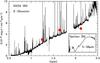 |
Fig. 2 X-shooter spectrum extracted at the HH34 IRS source position. Red dots correspond to the 2MASS photometry in the J,H, and K bands. The inset shows the mid-IR archival Spitzer-IRS spectrum. |
2. Observations
X-shooter observations of the HH34 IRS jet were conducted during the period November 2012–January 2013. Four different observations were acquired, each one integrated for 30 min on-source. The 11′′ slit was centered on the HH34 IRS source ( , δ = −06°26′58″) and aligned with the jet axis at PA 162° (see Fig. 1). The seeing during the observations was always between 0.̋6 and 1.̋0. Since the slit is filled with the emission from the jet, we performed off-source nodding for sky subtraction. Slit widths of 0.̋5, 0.̋4, and 0.̋4 were used for the UVB, VIS, and near-IR (NIR) arms, yielding resolutions of 9900, 18 200, and 7780, respectively. The pixel scale is 0.̋16 for the UVB and VIS arms, and 0.̋21 for the NIR arms. Data reduction was performed using the X-shooter pipeline version 2.2.0 (Modigliani et al. 2010), which provides 2D calibrated spectral images. Post-pipeline processing was performed using the IRAF1 package. This includes sky subtraction and telluric correction in the NIR images. To this end, the spectra of telluric standard stars acquired at similar airmass as the objects were used after the intrinsic photosperic features were removed. Finally, we combined the four different spectral images applying a median filter to get the final 2D spectral image.
Flux calibrations were performed within the pipeline using spectro-photometric standard stars acquired during the same night as the observations. In order to check for inter-calibration between the different arms, we extracted a spectrum of the HH34 IRS object in an aperture of 3′′ centered on-source and examined the continuum shape. Basically no continuum is detected shortward of 5000 Å, while there is a perfect match between the VIS and NIR arms in their overlapping region. However, comparing the NIR fluxes with the 2MASS photometry (Skrutskie et al. 2006) of the source we noticed that the X-shooter spectrum underestimates the NIR photometric points, likely because of slit losses due to the narrow slit width of the observations. A correct evaluation of the slit-losses should take into account the geometry of the continuum emission, as the source cannot be considered point-like owing to the presence of a diffuse nebulosity. We have instead re-scaled the X-shooter spectrum by a factor that minimizes the difference between the X-shooter fluxes and the 2MASS photometric points. The applied correction amounts to a factor of 2.7. However, as can be seen in Fig. 2, the shape of the 2MASS continuum is not reproduced well. This could be due to the presence of the diffuse nebulosity enhancing the J and H bands in the 2MASS large apertures, but also to source intrinsic variability.
Given the above discussion, we estimate that the relative flux calibration error between the three arms is very low, not more than 10%, while the absolute flux calibration is more uncertain and can be as high as 50%.
3. Results
As shown in Fig. 1, where the X-shooter slit is drawn over a [Fe ii] 1.64 μm image of the HH34 inner jet, our observations cover several emission peaks belonging to the blue-shifted jet (Antoniucci et al. 2014a). Separate spectra have been extracted from the 2D spectral images, corresponding to different regions selected from the intensity profiles of bright lines (see Fig. 1, right panel) – IRS, blue1, blue2, and blue3 – at progressively larger distances from the central object. These regions roughly comprise the knots called A3−A6 in previous studies (e.g., Garcia Lopez et al. 2008); however, given the large proper motion of these knots (see, e.g., Antoniucci et al. 2014a, and Sect. 3.1), we prefer to use a different nomenclature for our extraction regions that does not necessarily correspond to previously observed emission peaks.
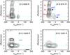 |
Fig. 3 Continuum-subtracted position velocity (PV) maps of [O i], [S ii], and [N ii] lines observed in the X-shooter spectrum. The PV are oriented along the jet, with a PA = 162°. Contours start at 3σ and are drawn at steps of 3σ with the exception of [S ii] 6731 Å where the contours are drawn in steps of 6σ. Radial velocities have been corrected for the source systemic velocity of +8 km s-1. The main peaks are labeled following the nomenclature of Fig. 1. The HVC and LVC are also indicated. |
The red-shifted counter-jet is clearly seen in the large-scale [Fe ii] image of Antoniucci et al (2014a). In Fig. 1 counter-jet emission is contaminated by the residuals of the PSF subtraction. However, in Garcia-Lopez et al. (2008) red-shifted emission is detected down to the central source. We therefore extract an additional spectrum, named red, comprising the counter-jet region close to the source.
Figure 2 shows the HH34 IRS complete spectrum. As expected for an embedded class I source, the spectrum sharply rises from UV to the infrared. Continuum and line emission are detected only above ~5000 Å . The X-shooter spectrum is also compared with a Spitzer-IRS spectrum taken from the Spitzer Heritage Archive (Program ORION_IRS, P.I. T. Megeath).
Strong emission lines are observed in the HH34 IRS spectrum, which are reported in Tables A.1−A.3, together with their identification and fluxes2. Lines detected in the other apertures are reported in Table A.4. Forbidden lines from abundant species originating in the jet are detected up to excitation energies of ~31 000 cm-1. In addition, we identify permitted lines from hydrogen (from the Brackett and Paschen series), helium, O i, Ca ii, and Na ii. Additional features, especially in the IR arm, do not have a clear identification, but the line shape and velocity widths suggest they are associated with metallic lines emitted in the same region as the other identified permitted lines. Finally, molecular lines from H2 and CO ro-vibrational transitions are also detected. The spectra extracted along the jet are, as expected, dominated by forbidden lines; however, Hα and Ca ii 8542 Å are also detected far from the central source. This is shown in Figs. 3−5, where the position-velocity (PV) diagrams of a few representative forbidden, permitted, and molecular transitions are presented. The local continuum has been removed by performing a linear fit through the emission adjacent to the lines. Since no photospheric lines of the source are detected − owing to the large veiling that fills all the absorption features – the source systemic velocity has been corrected for the velocity of the parental cloud (+8 km s-1, Anglada et al. 1995) after having corrected the spectra for the relative motion of Earth and Sun with respect to the standard of rest with the IRAF task rvcorrect.
Forbidden lines (e.g., [O ii], [S ii], [Fe ii], [N i]) have an extended blue-shifted component peaking at ~−100 km s-1 (hereafter high velocity, HV, or high velocity component, HVC) related to the jet. In addition, a spatially unresolved emission at lower velocity is also detected in all the lines (low velocity, LV, or low velocity component, LVC).
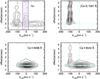 |
Fig. 4 As in Fig. 3 but for Hα and Ca ii lines. Contours start at 3σ and are drawn at steps of 3σ. The shadowed area in the Hα PV indicates a region with strong contamination from telluric residuals |
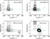 |
Fig. 5 As in Fig. 3 but for [Fe ii] and the H2 2.12 μm lines. Contours start at 3σ and are drawn at steps of 3σ, with the exception of 1.64 μm where the first five contours are at 2, 4, 6, 8, and 10σ to emphasize the red-shifted emission, and then continue at steps of 6σ. |
Finally a red-shifted HVC (Vr ~ + 130 km s-1) is clearly seen in the [Fe ii] 1.64 μm line. This component is not detected at shorter wavelengths and it is only barely detected in a few weaker [Fe ii] lines longward of 1.64 μm. We think this is due to the large extinction of the counter-jet. The non-detection of the 1.25 μm line set a lower limit on the extinction in the red-shifted component to AV> 13 mag, assuming the intrinsic 1.25 μm/1.64 μm ratio given in Giannini et al. (2015b) (see discussion in Sect. 4.1.2).
The above kinematical signatures were already known from previous [Fe ii] IR observations of HH34 (Garcia-Lopez et al. 2008; Antoniucci et al. 2008). We can now discuss any differences in the kinematical properties of lines having different excitation conditions.
To this end, we performed a Gaussian fitting to the line profile, from which the line Vpeak and velocity width were estimated. For the on-source spectrum, parameters for the HVC and LVC components were separately measured by fitting the line profile with two Gaussian components. Fluxes for all the lines derived from this Gaussian fitting are listed in Tables A.1−A.4, while Table 1 gives the kinematical parameters of a subsample of lines.
Peak velocities and width of selected lines.
From Table 1 and from the PV diagrams no shifts in the peak velocity of the HVC are appreciated within the errors, since Vr is ~(−100 ± 10) km s-1 for all the different lines, irrespective of their ionization stage or excitation temperature.
The jet velocity also remains fairly constant in all the extracted positions. Regarding the LVC, we observe that the peak velocity of [Fe ii] and [Ca ii] lines (~40−50 km s-1) is higher than for [S ii] and [O i] lines (~25−30 km s-1). This difference could be related to a large depletion of refractory elements at the lowest velocities. We discuss this aspect in Sect. 4.3.
No variations of the line widths are appreciable at the X-shooter resolution. However, we do see a decrease in ΔV values from the inner (ΔV ~ 50 ± 10 km s-1 on-source) to the outer (ΔV ~ 35 ± 10 km s-1 in blue2/3) knots.
Comparing the different PV diagrams, we note that high excitation lines (such as [N ii] 10407 Å and [S ii] 10320 Å, with Tex ~ 35 000−40 000 K) are spatially more compact than the other lines, as they are only detected within 2′′ of the source. The first emission peak is, for the majority of the lines, shifted by ~0.̋3 from the source position. Exceptions are [S ii] 6731 Å and [C ii]7291 Å, which have the first peak at about 0.̋7. As discussed in the next section, this is probably due to the low critical density of these lines, which are therefore quenched in the high density region closer to the star. Such a secondary peak is also seen in the [O i] line. At variance with the HVC, the LVC always peaks on-source.
Permitted lines, such as those of Ca ii, peak on-source at Vr ~ 0 km s-1. However, in the bright Ca ii line at 8542 Å the extended emission from the jet is also clearly detected, showing the same morphology and kinematics as the [Ca ii] 7291 Å emission. Such a jet emission is also detected in the Ca ii 8662 Å but not in the Ca ii 8498 Å line, probably owing to sensitivity. The Hα line presents a compact and very broad emission, which is largely self-absorbed at zero velocity, and an extended HV jet emission. Finally, H2 has kinematical signatures different from the atomic lines. The HVC component is prominent only at large distances from the central source (≳4′′), while the LVC is resolved and extends up to ±2′′ from the source. The H2 kinematics of HH34 has been presented and discussed in Garcia-Lopez et al. (2008) and is not further addressed here.
Offsets of emission peaks and tangential velocity.
3.1. Proper motion analysis
Observations of the HH34 jet over several decades have shown that the jet has a significant proper motion, with emission knots that change in position and morphology and new peaks that appear on timescales of a few years (Hartigan et al. 2011; Raga et al. 2012; Antoniucci et al. 2014a). Our PV data, compared with observations taken in different periods, can be used to measure the proper motions (PMs) of the knots close to the source. To this aim, we compare our data with those presented in Garcia Lopez et al. (2008), consisting of [Fe ii] spectra acquired with the ISAAC instrument (spatial sampling 0.̋146/pixel, thus comparable to that of the X-shooter VIS arm) in December 2004, i.e., 8 yr prior to our observations. We also used data with adequate spatial resolution, namely those of Davis et al. (2011; SINFONI [Fe ii] data from Oct. 2006, 0.̋05/pixel) and Antoniucci et al. (2014a; LBT [Fe ii] narrow band imaging, data from Apr. 2013, 0.̋118/pixel). In the latter data, only the region outside ~1′′ can be used owing to the contamination by residuals of the central source continuum deconvolution (see Fig. 1). Table 2 summarizes the shifts of the main emission components with respect to the central source position identified through the continuum fit.
The shifts on the X-shooter spectrum were measured from several bright lines, namely [O i] 6300 Å, [S ii] 6731 Å, [Ca ii] 7291 Å, [Fe ii] 8617 Å, and [Fe ii] 1.64 μm, and the results were averaged. In particular, we clearly identify three emission knots that can be associated with the knots A6, A5, and A3 of the Garcia Lopez et al. paper (see also Figs. 1 and 3). In addition, and as described before, the [S ii] 6731 Å and [Ca ii] 7291 Å lines present an emission peak at 0.̋7 that was not identified in previous ISAAC or SINFONI [Fe ii] observations; here we name it knot A6bis (indicated in Fig. 3). From Table 2, we see that knots A5 and A3 have moved during time: assuming the distance of 414 pc, the displacement corresponds to a tangential velocity of 270 and 200 km s-1 for the A5 and A3 knots, respectively. The PM of the HH34 jet has been measured by different authors. In particular Raga et al. (2012) compared different epoch HST observations deriving for the A5 and A3 HH34 jet knots a Vt comparable to our derived values (namely 250 and 210 km s-1).
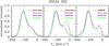 |
Fig. 6 Comparison of continuum subtracted line profiles extracted from the HH34 IRS spectrum. Line profiles are normalized to the peak of the HVC. |
We find, however, that inner knot A6 has not appreciably changed its position. The derived shift is compatible with the 0.̋2 shift measured by Garcia Lopez within the error, corresponding to an upper limit on the tangential velocity of <37 km s-1. Davis et al. (2011) measured a slightly lower offset, but their value is still compatible with the above upper limit.
The same A6 peak is present in observations taken in three different dates, which makes it very unlikely that we are seeing different ejections that are located by chance at the same offset during the observations. We can also exclude that the emission that we see is actually located on-source, but observed with an offset due to the large on-source extinction; in this case we would see a wavelength dependence of the offset while all the considered line peaks at the same position. The presence of stationary emission knots in the inner jet region is actually not a peculiar feature, as it has been already observed in other jets at different wavelengths, i.e., in DG Tau (offset 35−50 AU from source; Schneider et al. 2013; White et al. 2014), L1551-IRS5 (X-ray stationary emission at ~70 AU; Bonito et al. 2011), SVS13 ([Fe ii] 1.64 μm, emission at 20 AU from source; Davis et al. 2006). Such stationary structures are usually interpreted, in magneto-centrifugally driven jets, as shocks occurring at the jet recollimation region. In this framework, as the flow is launched outward, it enters a region where the magnetic tension toward the jet axis exceeds the centrifugal force so that the jet begins to recollimate at super-Alfvénic speeds, thus producing a shock region. In HH34 the stationary shock occurs at ~80−100 AU, thus at a distance larger than those observed in the other jets, but still consistent with models that predict that the recollimation shock region should be located at tens of AU above the circumstellar disk (e.g., Gomez de Castro & Pudritz 1993).
4. Jet physical conditions
The wealth of forbidden lines detected in the HH34 jet allows a detailed line diagnostic analysis to be performed on the gas physical conditions. Previous studies have already addressed the excitation conditions in the HH34 jet employing different set of diagnostic lines. Podio et al. (2006) considered several optical and IR lines to measure the electron density (ne), kinetic temperature (Te), and ionization fraction (xe) along the jet. Owing to the limited spatial resolution and sensitivity, the jet section below ~2′′ was not sampled and only large-scale variations of physical conditions were derived. Garcia Lopez et al. (2006) and Davis et al. (2011) used [Fe ii] IR lines to infer the electron density (ne) and extinction, and their variations with velocity, in the innermost jet knots. A more accurate analysis of the HH34 micro-jet is now possible by adopting lines of different species and excitation.
In the next section, we describe in detail the diagnostic analysis performed on the spectrum extracted at the source position, which is the richest in lines. This analysis allows us to investigate the properties in the initial ~0.̋5 section (~200 AU) where the jet shows a more complex kinematical behavior. In particular, we investigate any differences among the physical properties of the low and high velocity components. Variations of physical conditions in the other knots along the jet will be discussed in a separate section.
4.1. HH34-IRS jet base
4.1.1. Excitation trends as a function of velocity
Figure 6 shows the profiles of different forbidden lines extracted from the spectrum of the IRS position. Their comparison can be used to infer general trends on the difference in excitation between the high velocity jet and the component at lower velocity.
The left panel of Fig. 6 shows the profiles of four [Fe ii] lines that are sensitive to Te, ne, and Av variations (e.g., Nisini et al. 2005). In particular, the ratios [Fe ii]1.64 μm/1.25 μm and [Fe ii]1.64 μm/1.60 μm trace extinction and density variations, respectively. The normalized profiles of these three lines are remarkably similar and this agreement does not change with velocity, indicating that electron density and extinction remain constant in the HV and LV gas. On the other hand, the 1.64 μm/ 8617 Å line ratio decreases with increasing Te for a fixed density value: consequently, the observed profile variations with velocity suggests that the LVC is colder than the HVC.
The above trends are confirmed by the inspection of diagnostic lines from other species. The central panel of Fig. 6 shows the [Fe ii]1.64 μm line in comparison with different [S ii] lines. The [S ii]6716/6731 Å ratio, sensitive to ne, does not vary with velocity among the LVC and HVC, while the [S ii]10320/6731 Å, sensitive to Te, shows a decrease in the LV gas.
From inspection of Fig. 6 we also note that the [Fe ii]/[S ii] (central panel) and the [Fe ii]/[O i] (right panel) ratios decrease from the HVC to the LVC, irrespective of the considered [S ii] line. We interpret this as being due to a difference in the gas-phase Fe abundance in the two components, suggesting that Fe is more depleted on dust grains in the LVC emitting region than in the HVC region. The same behavior is observed in lines from other refractory species, like Ni and Ca (right panel of Fig. 6). This is discussed more quantitatively in Sect. 4.3.
4.1.2. Diagnostics analysis
The above qualitative considerations can be quantified by comparing the observed line fluxes, corrected for reddening, to statistical equilibrium NLTE codes under the assumption that the observed lines are optically thin. To this end, we made use of the NEBULIO database (Giannini et al. 2015a3).
We first consider the large number of [Fe ii] lines with different excitation conditions that can be used to derive the relevant parameters without any assumptions regarding elemental abundance. Giannini et al. (2013), have shown that owing to the uncertainty on the atomic parameters of the [Fe ii] lines, the best approach is statistical and implies including the largest number of line ratios in the analysis.
To this end, we fitted simultaneously all the lines detected with a signal to noise ratio higher than 5. The fit was performed separately for the HVC and LVC, whose relative fluxes – derived from a two-Gaussian fitting of the line profiles – are listed in Table A.1. In heavily embedded sources like HH34 IRS, it is of paramount importance to have a good determination of the extinction of the line emitting region, especially when ratios of lines in a wide wavelength range are considered. Extinction can be efficiently derived from the ratios of transitions sharing the same upper level so as to remove the dependence on the physical parameters influencing the level populations. Several [Fe ii] lines can be used for this and the 1.25 μm/1.64 μm intensity ratio involves the brightest ones. However, instead of using the theoretical radiative rate, which is affected by a large uncertainty (Bautista et al. 2013), we adopt the empirical determination of the radiative rate coefficients given in Giannini et al. (2015b). According to this work, the intrinsic [Fe ii] 1.25 μm/1.64 μm intensity ratio is between 1.11 and 1.2, from which we derive an on-source AV of 9.0 ± 0.5 mag, with no variations between the HVC and LVC.
We have consequently dereddened all the observed [Fe ii] lines assuming AV = 9 mag and adopting the extinction law of Cardelli et al. (1989). We have then compared these values against a grid of models in which the density varies from 103 to 108 cm-3 and the temperature from 3000 to 40 000 K.
Figure 7 shows the comparison between the observed intensities, normalized to the intensity of the 8616 Å line, with the theoretical ratios of the best-fit models for both the HVC and LVC. The best-fit models are ne ~ 5 × 104 cm-3, Te> 15 000 K for the HVC and ne ~ 5 × 104 cm-3, Te ~ 7000 K for the LVC. For the HVC, Fig. 7 shows that the model is not able to reproduce the lines with upper energy Eup> 15 000 cm-1. In fact, ratios of lines with high upper energy are systematically underestimated by up to an order of magnitude by the single-component model. These lines, originating from levels above the a4P term, have very high critical density (e.g., ncr ~ 107 cm-3 at Te = 10 000 K). Their excess emission could therefore be explained by the presence of an additional gas component at higher density. To test this hypothesis, we fitted the lines with Eup> 15 000 cm-1 separately. The considered ratios, involving both UV and IR lines, are very sensitive to extinction variations. Conversely, they are rather insensitive to temperature variations since they all have a similar excitation energy. In Fig. 8 we show χ2-contours obtained varying both density and AV values: within 90% of confidence AV varies between 8 and 10, while the density is larger than 106 cm-3.
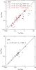 |
Fig. 7 [Fe II] observed vs. model predicted line intensities, normalized to the 8616 Å transition, relative to the HVC (top panel) and LVC (bottom panel). For the HVC, triangles refer to the model with a single gas component at ne = 5 × 104 cm-3 and Te > 15 000 K: filled (open) symbols indicate transitions with upper energies below (above) 15 000 cm-1. Red open circles refer to the model that includes an additional high density component with ne > 5 × 106 cm-3 to better fit the transitions at higher excitation energies. |
The relative contribution of the low and high density gas component in terms of emitting volume can be evaluated by comparing the absolute and dereddened observed fluxes with the emissivity values given by the model. We assume here that the emission of the 1.25 μm line is dominated by the low density gas, while the emission of the 5158 Å is dominated by the high density gas.
The ratio between the two emitting volumes – low density (LD) vs. high density (HD) components – is ~5000, for ne(HD) ~ 5 × 106 cm-3. Assuming a spherical emitting volume, the typical length scales are ~60 AU (0.̋15) for the LD component and ~3 AU (0.̋001) for the HD component. These values have at least a factor of two of uncertainty, considering both the uncertainty on calibration and extinction. Figure 7 shows the comparison between the observed and modeled ratios obtained by summing these two components with their relative filling factors.
In conclusion, the [Fe ii] analysis suggests the presence of an extended LD component with ne ~ 5 × 104 cm-3 and spatial scale ~60 AU (comparable to the length of the slit) and an unresolved (spatial scale 3AU) HD component with ne ≳ 106 cm-3. The ratio between the 5158 Å line observed on-source and in the blue 1 extracted spectrum is ~14, while the 8616 Å line has a comparable brightness in the two positions, which proves that the HD component represents a compact emission localized close to the source. The same is true for the 2.046 μm line, which is a factor of 10 brighter on-source with respect to the blue 1 position. The spatial resolution of our observations does not provide direct clues about the origin of this HD component. One possibility is that it traces a strong density gradient connected with the collimation shock region discussed in Sect. 3.1. Table 3 summarizes all the discussed physical parameters inferred from the Fe analysis.
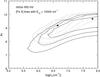 |
Fig. 8 χ2 contours of the fit through the [Fe ii] lines observed in the HVC and having Eup > 15 000 cm-1. Solid and dotted curves refer to Te = 10 000 K and 40 000 K, respectively. The curves refer to increasing values of χ2 of 30%, 60%, and 90%. The minimum χ2 value is indicated with a starred symbol. |
In addition to Fe, other forbidden lines can be used to derive independent estimates of the physical conditions. We combined, in particular, [S ii] transitions at 6716, 6731, and 1.03 μm to infer ne and Te (see Fig. 9).
Table 3 includes the results of all the above diagnostic analysis. Temperatures inferred from [S ii] for the HVC and LVC are in agreement with the values derived from the [Fe ii] analysis, while the values of the density are slighter lower. This is indeed a general result in stellar jets (e.g., Giannini et al. 2013; Podio et al. 2006; Nisini et al. 2005) and it is due to the low critical density of the [S ii] lines making them more sensitive to low density regions when density gradients are present.
Constraints on the ionization fraction can be also obtained from the upper limit on the [O ii] 7329 Å and [Fe iii] 5270 Å lines, and from the [N i] 5198/[N ii] 6583 Å detected ratio. Adopting the ionization equilibrium model described in Giannini et al. (2015a), only upper limits on the ionization fraction can be inferred, and all the methods indicate a low xe value (see Table 3). The most stringent upper limit is found from the [N i]/[N ii] ratio which is consistent with xe < 0.1.
From the xe upper limit we derive a lower limit on the total density nH > 5 × 105 cm-3 in the HVC. This value can be used to infer the jet mass loss rate by directly measuring the mass flowing through a jet annulus, namely  . Here, μ = 1.24 is the average atomic weight, rJ the jet radius, and VJ the jet velocity. This method assumes that the jet section is completely filled with gas at the considered total density. The value of VJ is taken equal to 290 km s-1, as derived from combining the jet radial and tangential velocities discussed in Sect. 3. The value of rJ is assumed equal to the width of the [Fe ii] emission as measured by Davis et al. (2011), namely ~0.̋1 (~40 AU). With a total density of 5 × 105cm-3, Ṁjet = 5 × 10⁻⁷M⊙ yr-1 is derived. This value is comparable with that derived by Podio et al. (2006) at a few arcsec distance from the source adopting the same method, while it is higher by an order of magnitude than the value estimated by Garcia Lopez et al. (2008) on the same spatial scale from the luminosity of the [Fe ii] lines. This method, however, is subject to more uncertainties as it strongly depends on the adopted extinction value, on flux losses within the slit, and on the exact iron depletion factor in the jet. The derived mass flux rate implies that the source mass accretion rate should be at least >10-6M⊙ yr-1 to find consistency with any of the jet formation models predicting Ṁjet/Ṁacc < 0.5 (Ferreira et al. 2006). This point is further discussed in Sect. 5.
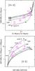 |
Fig. 9 Diagnostic diagrams employing density and temperature sensitive ratios of [Fe ii] and [S ii] transitions. Observed ratios, dereddened assuming the AV values given in Table 3, are shown as purple symbols. |
Derived physical parameters.
4.2. Variation of physical parameters along the jet
The analysis performed on the IRS spectrum was also applied on the other extracted knots in order to follow the variations of physical parameters along the jet. In summary, we performed the [Fe ii] line fit and used the [S ii] diagnostic analysis as described in the previous section for deriving the AV, ne, and Te values. However, significant constraints on xe cannot be derived along the jet since the limits on the involved line ratios are not stringent enough. Table 3 summarizes the obtained values, while Fig. 9 presents [Fe ii] and [S ii] diagnostic diagrams compared with dereddened line ratios that illustrate how the physical parameters vary from knot to knot.
From Fig. 9 and Table 3 we see that electron density and temperature decrease from the inner to the outer knots, a trend already observed in jets from T Tauri stars (e.g., Lavalley-Fouquet et al. 2000; Podio et al. 2009; Maurri et al. 2014) and from Class I sources (Bacciotti & Eisloffel 1999; Nisini et al. 2005; Podio et al. 2006).
Garcia Lopez et al. (2008) derived the electron density along the HH34 jet using the [Fe ii] 1.64/1.60 μm line ratio. They find a difference in density between the HVC and LVC, i.e., the LVC density higher by a factor of two with respect to the HVC, which we do not see in our data. This is probably due to the different extraction regions of the two data sets. In Garcia Lopez et al., their A6 knot comprises our IRS, blue 1, and blue 2 extractions (i.e., about 3′′). Therefore, their HVC density, averaged over a large region at progressively decreasing density, is lower than our derived value by a factor of 5. In contrast, the LVC component is compact and not resolved in both of the observations; therefore, the two density values are more similar (2.2 × 10⁴ against 5 × 104 cm-3).
In general, we find density values higher by a factor of ~2 with respect to the Garcia Lopez et al. values. We think this difference is due to the different aperture sizes and also to the use of a larger number of lines from different [Fe ii] levels sensitive to higher density conditions.
4.3. Iron depletion
As shown in Sect. 4.1, intensity variations with velocities observed on the line profiles suggest that the abundances of refractory elements, like [Fe ii], [Cr ii], and [Ni ii], decreases in the LVC as compared with the high velocity gas. These elements in gas phase can be underabundant with respect to solar values owing to depletion on dust grains. In fact, a measure of the gas phase depletion of refractory species such as Fe offers a direct indication of the presence of dust in the emitting region, and hence makes it possible to determine whether the outflowing material originates inside or outside the dust sublimation radius. Previous estimates of the Fe gas phase abundance in jets indicate depletion factors ranging between 20 to 80% with respect to solar values (Nisini et al. 2002; 2005; Podio et al. 2006; Giannini et al. 2013) at distances larger than ~400 AU from the source. Agra-Amboage et al. (2011) measured the iron depletion in the DG Tau jet down to 50 AU from the source. They found a depletion of a factor ~ 3 in the high velocity component and a factor ~ 10 at velocities <100 km s-1. The HH34 observations probe the jet within ~200 AU from the source and thus our iron abundance estimates can be compared reasonably well with those of DG Tau.
Iron depletion can be measured by comparing [Fe ii] fluxes with those of lines from species that show no depletion onto grains. These reference lines should be emitted in the same volume of gas as the [Fe ii] lines. To this end, infrared [Fe ii] lines have been in the past compared with IR [P ii] lines in HH objects and jets (e.g., Nisini et al. 2005) as the IR transitions of the two species share similar excitation conditions. In the optical, a suitable ratio is the [Fe ii]8616 Å/[O i] 6300 Å since these two lines show similar PV diagrams and are close enough in wavelength to minimize errors induced by AV uncertainties. The use of this ratio also implies assuming that oxygen is mostly neutral and iron mostly ionized, an assumption confirmed by the low ionization fraction derived.
In Fig. 10 we plot the [Fe ii] 8616 Å/[O i] 6300 Å expected ratio as a function of the gas temperature, for the density value derived in the HH34 IRS region. Different curves are plotted that assume a relative [Fe/O] solar abundance of 0.062 (Asplund et al. 2006) and decreasing fractions of this value. The values derived from the observations in the HVC and LVC are shown with their errors. The HVC is consistent with the solar abundance value and Te ~ 15 000 K. For the LVC, a larger error is given on the [Fe ii]/[O i] ratio that is due to the contamination of the [O i] 6300Å line by residuals of the telluric line subtraction. The gas phase [Fe/O] value derived for this component implies Fe depletion of a factor between 2 and 8 with respect to solar.
We therefore find results consistent with the DG Tau case where the [Fe ii] depletion in the LVC is larger than in the HVC. A similar depletion pattern as a function of velocity has also been found from the analysis of other refractory species, e.g., Ca (e.g., Podio et al. 2009). As discussed in Agra-Amboage et al. (2011), this implies that the low velocity gas originates from a region located at a larger distance from the star and/or from a region where the dust has been less shock-reprocessed. At variance with the DG Tau case, however, we do not see a significant iron depletion in the high velocity gas.
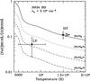 |
Fig. 10 [Fe ii] 8616 Å/[O i] 6300 Å ratio plotted against the gas temperature for a density of 5 × 104 cm-3. The solid curve shows predictions assuming an [Fe/O] solar gas phase abundance of 0.062 (Asplund et al. 2006). Other curves are plotted for decreasing values of the [Fe/O] abundance. Data points correspond to the values measured in the HVC and LVC toward HH34 IRS, and indicate an [Fe/O] abundance ratio close to solar for the HVC and a factor between 2 and 8 below solar for the LVC. |
5. Mass accretion rate
The on-source spectrum of HH34 presents several optical and IR permitted lines that are often used as proxies for the accretion luminosity (Lacc) in young stars. Among the brightest are the HI (Hα, Paβ, Brγ), OI (8446.4 Å), and Ca II (8498 Å, 8542 Å, 8662 Å) transitions. Although the real origin of these lines – whether in accretion columns and spots, or in ionized winds – is still uncertain, it has been shown that their intrinsic luminosity scales with Lacc in T Tauri stars (Herczeg & Hillenbrand 2008; Alcalá et al. 2014). As such they have been widely used to indirectly derive Lacc and consequently the mass accretion rate (Ṁacc) in sources with known stellar parameters (e.g., Antoniucci et al. 2014b). Using the assumption that the same relationships between Lline vs. Lacc also hold in the more embedded class I sources, we can estimate Ṁacc in HH34 IRS from the dereddened line luminosities. The main uncertainty in this procedure is the knowledge of the extinction value in regions close to the source where the permitted lines originate.
A direct estimate of the on-source extinction value can be gathered by the depth of absorption bands detected in the Spitzer-IRS on-source spectrum (see Fig. 2). In particular, the silicate absorption feature at 9.7 μm can be used by adopting the relationship AV/τ9.7 = 18.5 ± 1.5 mag from Mathis (1998). This gives an AV value between 30 and 33 mag. A high value of AV is also estimated by Antoniucci et al. (2008), who applied a self-consistent method to simultaneously derive AV, Lacc, and L∗ in HH34 IRS from the source bolometric luminosity, IR magnitudes, and Brγ flux. They infer an AV value close to 50 mag and a Ṁacc of 4.1 × 10⁻⁶M⊙ yr-1. Hence the permitted lines might originate in a region more deeply embedded than the jet region where the forbidden lines are located.
Taking advantage of the wide wavelength range covered by our data, in principle we can derive simultaneously AV and Ṁacc by considering the AV that gives consistent Ṁacc values from the different dereddened line luminosities (in particular Hα, O i8446 Å, Ca ii8662 Å, Paβ, and Brγ). Applying this method, and using the empirical relationships between Lline and Lacc derived by Alcalá et al. (2014), we find AV = 7 mag and Ṁacc = (8 ± 7) 10-9M⊙ yr-1 (assuming M∗ = 0.5 M⊙ and considering absolute calibration errors on the line luminosity).
The AV derived in this way is much lower than that measured from the silicate band and the Ṁacc value is two order of magnitudes lower than the jet mass flux rate. In addition, following the arguments of Antoniucci et al. (2008), such a low mass accretion rate would imply that the bolometric luminosity of the central source (12−20 L⊙) is not accretion dominated, but rather dominated by the stellar photosphere. However, this is not consistent with the source IR photometry and AV = 7 mag value for any central star spectral type.
A possible explanation for this discrepancy could be that a significant fraction of the permitted line emission originating very close to the star is seen here as emission scattered in the cavity excavated envelope. The net effect of scattering would be to enhance the line emission at shorter wavelengths with respect to the IR lines, with a wavelength dependent law different from the adopted reddening law. We therefore conclude that the relationships between accretion luminosity and permitted optical line luminosity derived for T Tauri stars cannot be directly extended to class I sources embedded in reflection nebulae.
An alternative way to indirectly estimate the mass accretion rate is to use empirical correlations between Ṁacc and the luminosity of forbidden lines. For example, Herczeg & Hillenbrand (2008) found a correlation between the [O i] 6300 Å luminosity and the accretion luminosity in T Tauri stars. This relationship has been used to infer the mass accretion rates in embedded objects or in edge-on-disk T Tauri where the permitted line emission is partially hidden at a direct view (Whelan et al. 2014; Riaz et al. 2015). However, the [O i] emission in the Herczeg & Hillenbrand sample was dominated by the low velocity wind component. Nisini et al. (in prep.) revised this correlation for a sample of CTTs of the Lupus and Cha clouds, considering only the [O i] 6300Å luminosity in the HVC. They found the following relationship: log (L[O i] HVC) = 0.8 log (Ṁacc) + 1.8. Assuming that the same relationship holds also for class I sources, for HH34 IRS we derive Ṁacc = (7.5 ± 4) 10-6M⊙ yr-1. This is close to the value originally derived by Antoniucci et al. (2008) and implies a Ṁjet/Ṁacc ~ 0.1, i.e., well within the range expected for magneto-centrifugally jet launching models (Ferreira et al. 2006).
6. Discussion and conclusions
In this section we summarize and discuss the main results found from the analysis of the X-shooter spectrum of the HH34 IRS micro-jet.
6.1. Kinematics vs. excitation
Thanks to the large spectral coverage and sensitivity reached by the X-shooter observations, we were able to detect lines spanning a wide range of excitation energies (from ~8000 to ~31 000 cm-1) and critical densities (from ~103 to ~107 cm-3). We find that PV diagrams of lines with different excitation conditions are remarkably similar. The peak velocity and the FWHM of the HVC is the same for all lines, even though – at least in the on-source position – high excitation lines seem to trace a denser gas. Hence density stratifications are not associated with different velocity components. In particular, we do not see evidence at our spectral resolution that high velocity material located close to the jet axis, has higher density than the jet streamlines at lower velocities on the border. This is in contrast with the onion-like structure predicted by the theoretical model and confirmed by high resolution observations of CTT jets (e.g., Maurri et al. 2014), and may be due to the lack of angular resolution: in regions more distant from the driving source (like those probed here), shocks may have already destroyed the jet’s onion-like structure. With regard to the spatial variations, all transitions peak at the same offsets from the source with the exception of the [S ii] and [Ca ii] lines, which – having critical densities <5 × 103 cm-3 – are probably quenched in the high density knots close to the star. We therefore conclude that shock layers at different excitation behind the shock front are not spatially resolved.
6.2. Physical parameters, mass loss rate, and comparison with properties of CTT stars
Our study presents the first estimates of the full set of physical parameters (ne, Te, xe, nH) in the initial 200 AU of a jet from an embedded class I source. The values found in this inner jet are Te ≳ 15 000 K, ne ~ 5 × 104 cm-3, and fractional ionization xe < 0.1, which implies a total density nH > 5 × 105 cm-3. A gas component whose density is at least two order of magnitudes higher is also suggested by the intensity of the [Fe ii] lines at higher excitation. However, this component does not contribute to more than 1% of the jet mass if we assume for it the same fractional ionization as the lower density gas.
Although the results derived from this single source cannot be generalized to all the class I objects, it is instructing to compare the derived parameters with values typically found in CTTs jets, especially for the fractional ionization and total density, the parameters derived here for the first time.
The total density estimated in the HH34 jet (nH > 5 × 105 cm-3) is at the upper boundary of the typical values found in CTTs on the same spatial scales of our observations. Values in the range 104−105 cm-3 are derived in DG Tau, HH30, and RW Aur (Maurri et al. 2014; Hartigan & Morse 2007; Melnikov et al. 2009), which are among the most active CTTs.
Fractional ionizations in CTT jets have strong gradients in the initial ~150 AU from the source. In DG Tau, for example, the ionization fraction increases from ~0.07 at the jet base to up to 0.6−0.8 above 150 AU (Maurri et al. 2007). Similarly, in HH30, xe is ≲0.1 within 50 AU of the source, and then progressively increases up to ~0.3 at about 200 AU (Hartigan & Morse 2007). We do not have the spatial resolution to see xe variations in this inner jet sections and we measure xe < 0.1 as an average value of the region where such strong gradients are expected. Podio et al. (2006) have also shown that xe in HH34 never rises above 0.1 at large distances. Such low values of fractional ionizations, however, are found in the jet from RW Aur, where xe ~ 0.1 has been measured along the entire micro-jet up to distances of few arcsec (Melnikov et al. 2009). In gas excited by shocks, low values of fractional ionization are expected either for low shock velocity or for high pre-shock density. Since the HH34 jet velocity and velocity spread are similar to other T Tauri stars where higher ionization has been found, the low xe value is probably a direct consequence of the high density in the jet.
The mass flux rate derived from the estimated value of the total density is Ṁjet > 5 × 10⁻⁷M⊙ yr-1. This is at least an order of magnitude higher than values measured on active T Tauri stars (see, e.g., Ellerbroek et al. 2013). We therefore conclude that the class I HH34 IRS jet shares many kinematical and physical properties with the most active CTTs stars, but its density and mass flux is at least an order of magnitude higher.
6.3. Origin of the LVC
The LVC at the source position is detected in all the brightest lines and it is blue-shifted by ~30−50 km s-1. From the diagnostic analysis it results that the LVC shares the same electron density and extinction as the base of the HVC, but has a lower temperature, on the order of ~7000 K. Forbidden line emission components centered close to systemic velocity are features commonly observed in CTT stars (e.g., Hartigan et al. 1995; Natta et al. 2014). The typical peak velocities of CTT LVCs are in the range ~5−20 km s-1 (thus closer to systemic velocity than the HH34 LVC) and they are usually brighter than the corresponding HVC emission, even in sources known to drive prominent jets (e.g., Hartigan et al. 1995). As we estimate a similar extinction between the HVC and LVC, the weakness of the LVC cannot be attributed to an origin in a region more embedded than the high velocity jet gas emission. The origin of the LVC is unclear: in CTTs it has been attributed either to low velocity magnetically driven disk-winds or to winds photo-evaporated by UV or X-ray photons from the central star. An origin in photo-evaporated wind is very unlikely in the HH34 IRS case, because the peak velocity appears much more blue-shifted than in the line profiles predicted by models (e.g., Ercolano & Owen 2010) and because it is conceivable that any stellar high energetic photon would be absorbed by the dense jet before being able to photoevaporate disk material. It is therefore more likely that the LVC originates from a slow magnetically accelerated disk-wind. Different flow acceleration models do indeed predict the formation of compact slow winds.
Romanova et al. (2009), for example, provide numerical simulations of outflows launched from the interaction region between the disk and a rotating magnetized star, which in principle could explain the presence of a LVC. This model predicts the formation of a fast axial-symmetric jet and of a conical inner wind powered by the magnetic pressure force. Romanova et al. (2009) applied their simulations to different types of stars. For the case of class I sources relevant here, the protostar is assumed to be rapidly rotating causing the formation of an energetic jet that carries away a relevant amount of angular momentum and of a slow conical wind with poloidal velocities up to 50 km s-1. Thus, the model could explain the kinematics we observe in our data. However the conical wind is predicted to be at higher density with respect to the jet, which is contradicted by our analysis. In addition, the wind is formed in the inner disk region close to the star: this is not consistent with the [Fe ii] depletion we observe in the LVC, which suggests a formation in a disk region where the dust has not sublimated yet.
A different class of models are those that consider an outflow originating from a magnetized disk (e.g., Konigl & Pudritz 2000; Ferreira et al. 2006). In these models the wind is ejected from an extended range of radii and thus they naturally predict components at different velocities as arising in flows from different streamlines at decreasing poloidal velocity across the disk. Extended MHD disks can also take into account the [Fe ii] depletion pattern as the gas at low velocity is likely ejected from large disk radii, outside the dust sublimation radius. This class of models also predicts that the particle density should decrease along the radial streamlines, a feature in apparent contradiction with our finding of constant electron density. However, the total density could still be consistent with the predicted pattern if the ionization fraction in the LVC is smaller than in HVC. In this respect, we point out that a decrease in the fractional ionization with velocity has been observed in T Tauri stars (e.g., Maurri et al. 2014).
6.4. Mass accretion rate in class I sources
The luminosity of optical/IR permitted lines is routinely used to measure the accretion luminosity and thus accretion rates in CTT stars adopting empirical relationships calibrated on samples of stars with known accretion luminosity, derived, for example, from the UV veiling and Balmer jump. In embedded sources, where the UV spectral region is not directly accessible, the possibility to use these empirical relationships would provide a very important tool to obtain information on the accretion properties of the sources. However, the analysis we have performed on source HH34 IRS shows that the optical lines are likely seen through scattered light and thus their intrinsic luminosity cannot be retrieved by adopting a standard reddening law. Methods that self-consistently infer both Ṁacc and AV combining Brγ line luminosity and stellar parameters, as adopted in Antoniucci et al. (2008), seem better able to infer the accretion properties for these objects. This method, however, relies on a good knowledge of the source bolometric luminosity.
Empirical relationships correlating Ṁacc with the luminosity of forbidden lines, such as the [O i] line, can also be used to estimate the mass accretion rate. These relationships, calibrated on CTT stars, hinges on the connection between [O i] luminosity and mass ejection rate, which in turn indirectly depends on the mass accretion rate. Therefore, its goodness eventually relies on the assumption that the HH34 IRS jet shares a similar mass ejection efficiency to that of T Tauri stars.
Ultimately, however, for better accretion proxy in class I sources not contaminated by scattered light and less dependent on extinction, it is necessary to go into the mid-IR regime. Examples of studies toward that direction are those of Salyk et al. (2013) who used the Pfβ luminosity, and Rigliaco et al. (2015), who explored the potential of the HI(7−6) at 12.37 μm.
IRAF is distributed by the National Optical Astronomy Observatory, which is operated by the Association of Universities for Research in Astronomy (AURA) under a cooperative agreement with the National Science Foundation.
Transition wavelengths in Table 1 are air wavelengths expressed in Angstrom. In the paper, we refer for convenience to lines in Angstrom or in μm depending on whether they are below or above 1 micron.
Acknowledgments
This project was financially supported by the PRIN INAF 2012 “Disks, jets and the dawn of planets”. L.P. has received funding from the European Union Seventh Framework Programme (FP7/2007−2013) under grant agreement No. 267251.
References
- Agra-Amboage, V., Dougados, C., Cabrit, S., & Reunanen, J. 2011, A&A, 532, A59 [NASA ADS] [CrossRef] [EDP Sciences] [Google Scholar]
- Alcalá, J. M., Natta, A., Manara, C. F., et al. 2014, A&A, 561, A2 [NASA ADS] [CrossRef] [EDP Sciences] [Google Scholar]
- Anglada, G., Estalella, R., Mauersberger, R., et al. 1995, ApJ, 443, 682 [NASA ADS] [CrossRef] [Google Scholar]
- Antoniucci, S., Nisini, B., Giannini, T., & Lorenzetti, D. 2008, A&A, 479, 503 [NASA ADS] [CrossRef] [EDP Sciences] [Google Scholar]
- Antoniucci, S., La Camera, A., Nisini, B., et al. 2014a, A&A, 566, A129 [NASA ADS] [CrossRef] [EDP Sciences] [Google Scholar]
- Antoniucci, S., García López, R., Nisini, B., et al. 2014b, A&A, 572, A62 [NASA ADS] [CrossRef] [EDP Sciences] [Google Scholar]
- Asplund, M., Grevesse, N., & Jacques Sauval, A. 2006, Nucl. Phys. A, 777, 1 [NASA ADS] [CrossRef] [Google Scholar]
- Bacciotti, F., & Eislöffel, J. 1999, A&A, 342, 717 [NASA ADS] [Google Scholar]
- Bacciotti, F., Whelan, E. T., Alcalá, J. M., et al. 2011, ApJ, 737, L26 [NASA ADS] [CrossRef] [Google Scholar]
- Bautista, M. A., Fivet, V., Quinet, P., et al. 2013, ApJ, 770, 15 [NASA ADS] [CrossRef] [Google Scholar]
- Beck, T. L., Riera, A., Raga, A. C., & Reipurth, B. 2007, AJ, 133, 1221 [NASA ADS] [CrossRef] [Google Scholar]
- Bonito, R., Orlando, S., Miceli, M., et al. 2011, ApJ, 737, 54 [CrossRef] [Google Scholar]
- Cardelli, J. A., Clayton, G. C., & Mathis, J. S. 1989, ApJ, 345, 245 [NASA ADS] [CrossRef] [Google Scholar]
- Davis, C. J., Whelan, E., Ray, T. P., & Chrysostomou, A. 2003, A&A, 397, 693 [NASA ADS] [CrossRef] [EDP Sciences] [Google Scholar]
- Davis, C. J., Nisini, B., Takami, M., et al. 2006, ApJ, 639, 969 [NASA ADS] [CrossRef] [Google Scholar]
- Davis, C. J., Cervantes, B., Nisini, B., et al. 2011, A&A, 528, A3 [NASA ADS] [CrossRef] [EDP Sciences] [Google Scholar]
- Ellerbroek, L. E., Podio, L., Kaper, L., et al. 2013, A&A, 551, A5 [NASA ADS] [CrossRef] [EDP Sciences] [Google Scholar]
- Ercolano, B., & Owen, J. E. 2010, MNRAS, 406, 1553 [NASA ADS] [Google Scholar]
- Ferreira, J., Dougados, C., & Cabrit, S. 2006, A&A, 453, 785 [NASA ADS] [CrossRef] [EDP Sciences] [Google Scholar]
- Frank, A., Ray, T. P., Cabrit, S., et al. 2014, Protostars and Planets VI, 451 [Google Scholar]
- Garcia Lopez, R., Nisini, B., Giannini, T., et al. 2008, A&A, 487, 1019 [NASA ADS] [CrossRef] [EDP Sciences] [Google Scholar]
- Garcia Lopez, R., Nisini, B., Eislöffel, J., et al. 2010, A&A, 511, A5 [NASA ADS] [CrossRef] [EDP Sciences] [Google Scholar]
- Giannini, T., Nisini, B., Antoniucci, S., et al. 2013, ApJ, 778, 71 [NASA ADS] [CrossRef] [Google Scholar]
- Giannini, T., Antoniucci, S., Nisini, B., Bacciotti, F., & Podio, L. 2015a, ApJ, 814, 52 [NASA ADS] [CrossRef] [Google Scholar]
- Giannini, T., Antoniucci, S., Nisini, B., et al. 2015b, ApJ, 798, 33 [NASA ADS] [CrossRef] [Google Scholar]
- Gomez de Castro, A. I., & Pudritz, R. E. 1993, ApJ, 409, 748 [NASA ADS] [CrossRef] [Google Scholar]
- Hartigan, P., & Morse, J. 2007, ApJ, 660, 426 [NASA ADS] [CrossRef] [Google Scholar]
- Hartigan, P., Edwards, S., & Ghandour, L. 1995, ApJ, 452, 736 [NASA ADS] [CrossRef] [Google Scholar]
- Hartigan, P., Frank, A., Foster, J. M., et al. 2011, ApJ, 736, 29 [Google Scholar]
- Herczeg, G. J., & Hillenbrand, L. A. 2008, ApJ, 681, 594 [NASA ADS] [CrossRef] [Google Scholar]
- Konigl, A., & Pudritz, R. E. 2000, Protostars and Planets IV, 759 [Google Scholar]
- Lavalley-Fouquet, C., Cabrit, S., & Dougados, C. 2000, A&A, 356, L41 [NASA ADS] [Google Scholar]
- Mathis, J. S. 1998, ApJ, 497, 824 [NASA ADS] [CrossRef] [Google Scholar]
- Maurri, L., Bacciotti, F., Podio, L., et al. 2014, A&A, 565, A110 [NASA ADS] [CrossRef] [EDP Sciences] [Google Scholar]
- Melnikov, S. Y., Eislöffel, J., Bacciotti, F., Woitas, J., & Ray, T. P. 2009, A&A, 506, 763 [NASA ADS] [CrossRef] [EDP Sciences] [Google Scholar]
- Modigliani, A., Goldoni, P., Royer, F., et al. 2010, Proc. SPIE, 7737, 773728 [Google Scholar]
- Natta, A., Testi, L., Alcalá, J. M., et al. 2014, A&A, 569, A5 [NASA ADS] [CrossRef] [EDP Sciences] [Google Scholar]
- Nisini, B., Caratti o Garatti, A., Giannini, T., & Lorenzetti, D. 2002, A&A, 393, 1035 [Google Scholar]
- Nisini, B., Bacciotti, F., Giannini, T., et al. 2005, A&A, 441, 159 [NASA ADS] [CrossRef] [EDP Sciences] [Google Scholar]
- Podio, L., Bacciotti, F., Nisini, B., et al. 2006, A&A, 456, 189 [NASA ADS] [CrossRef] [EDP Sciences] [Google Scholar]
- Podio, L., Medves, S., Bacciotti, F., Eislöffel, J., & Ray, T. 2009, A&A, 506, 779 [NASA ADS] [CrossRef] [EDP Sciences] [Google Scholar]
- Raga, A. C., Noriega-Crespo, A., Lora, V., Stapelfeldt, K. R., & Carey, S. J. 2011, ApJ, 730, L17 [NASA ADS] [CrossRef] [Google Scholar]
- Raga, A. C., Noriega-Crespo, A., Rodríguez-González, A., et al. 2012,ApJ, 748, 103 [Google Scholar]
- Ray, T., Dougados, C., Bacciotti, F., Eislöffel, J., & Chrysostomou, A. 2007, Protostars and Planets V, 231 [Google Scholar]
- Reipurth, B., Heathcote, S., Morse, J., Hartigan, P., & Bally, J. 2002, AJ, 123, 362 [NASA ADS] [CrossRef] [Google Scholar]
- Riaz, B., Thompson, M., Whelan, E. T., & Lodieu, N. 2015, MNRAS, 446, 2550 [NASA ADS] [CrossRef] [Google Scholar]
- Rigliaco, E., Pascucci, I., Duchene, G., et al. 2015, ApJ, 801, 31 [NASA ADS] [CrossRef] [Google Scholar]
- Romanova, M. M., Ustyugova, G. V., Koldoba, A. V., & Lovelace, R. V. E. 2009, MNRAS, 399, 1802 [NASA ADS] [CrossRef] [Google Scholar]
- Salyk, C., Herczeg, G. J., Brown, J. M., et al. 2013, ApJ, 769, 21 [NASA ADS] [CrossRef] [Google Scholar]
- Schneider, P. C., Eislöffel, J., Güdel, M., et al. 2013, A&A, 557, A110 [NASA ADS] [CrossRef] [EDP Sciences] [Google Scholar]
- Shang, H., Li, Z.-Y., & Hirano, N. 2007, Protostars and Planets V, 261 [Google Scholar]
- Skrutskie, M. F., Cutri, R. M., Stiening, R., et al. 2006, AJ, 131, 1163 [NASA ADS] [CrossRef] [Google Scholar]
- Takami, M., Chrysostomou, A., Ray, T. P., et al. 2006, ApJ, 641, 357 [NASA ADS] [CrossRef] [Google Scholar]
- Vernet, J., Dekker, H., D’Odorico, S., et al. 2011, A&A, 536, A105 [NASA ADS] [CrossRef] [EDP Sciences] [Google Scholar]
- Whelan, E. T., Bonito, R., Antoniucci, S., et al. 2014, A&A, 565, A80 [NASA ADS] [CrossRef] [EDP Sciences] [Google Scholar]
- White, M. C., McGregor, P. J., Bicknell, G. V., Salmeron, R., & Beck, T. L. 2014, MNRAS, 441, 1681 [NASA ADS] [CrossRef] [Google Scholar]
Appendix A: Tables of line fluxes
Lines observed in the on-source extraction: the HV and LV components.
Lines observed in the on-source extraction: permitted lines.
Lines observed on-source: molecular lines.
Forbidden lines observed along the jet.
All Tables
All Figures
|
Fig. 1 Left: adopted X-shooter slit over a [Fe II] 1.64 μm narrow band image of the HH34 jet obtained with LBT-LUCI (Antoniucci et al. 2014a). The blue circle indicates the source position at α = 05h35m29 |
| In the text | |
|
Fig. 2 X-shooter spectrum extracted at the HH34 IRS source position. Red dots correspond to the 2MASS photometry in the J,H, and K bands. The inset shows the mid-IR archival Spitzer-IRS spectrum. |
| In the text | |
|
Fig. 3 Continuum-subtracted position velocity (PV) maps of [O i], [S ii], and [N ii] lines observed in the X-shooter spectrum. The PV are oriented along the jet, with a PA = 162°. Contours start at 3σ and are drawn at steps of 3σ with the exception of [S ii] 6731 Å where the contours are drawn in steps of 6σ. Radial velocities have been corrected for the source systemic velocity of +8 km s-1. The main peaks are labeled following the nomenclature of Fig. 1. The HVC and LVC are also indicated. |
| In the text | |
|
Fig. 4 As in Fig. 3 but for Hα and Ca ii lines. Contours start at 3σ and are drawn at steps of 3σ. The shadowed area in the Hα PV indicates a region with strong contamination from telluric residuals |
| In the text | |
|
Fig. 5 As in Fig. 3 but for [Fe ii] and the H2 2.12 μm lines. Contours start at 3σ and are drawn at steps of 3σ, with the exception of 1.64 μm where the first five contours are at 2, 4, 6, 8, and 10σ to emphasize the red-shifted emission, and then continue at steps of 6σ. |
| In the text | |
|
Fig. 6 Comparison of continuum subtracted line profiles extracted from the HH34 IRS spectrum. Line profiles are normalized to the peak of the HVC. |
| In the text | |
|
Fig. 7 [Fe II] observed vs. model predicted line intensities, normalized to the 8616 Å transition, relative to the HVC (top panel) and LVC (bottom panel). For the HVC, triangles refer to the model with a single gas component at ne = 5 × 104 cm-3 and Te > 15 000 K: filled (open) symbols indicate transitions with upper energies below (above) 15 000 cm-1. Red open circles refer to the model that includes an additional high density component with ne > 5 × 106 cm-3 to better fit the transitions at higher excitation energies. |
| In the text | |
|
Fig. 8 χ2 contours of the fit through the [Fe ii] lines observed in the HVC and having Eup > 15 000 cm-1. Solid and dotted curves refer to Te = 10 000 K and 40 000 K, respectively. The curves refer to increasing values of χ2 of 30%, 60%, and 90%. The minimum χ2 value is indicated with a starred symbol. |
| In the text | |
|
Fig. 9 Diagnostic diagrams employing density and temperature sensitive ratios of [Fe ii] and [S ii] transitions. Observed ratios, dereddened assuming the AV values given in Table 3, are shown as purple symbols. |
| In the text | |
|
Fig. 10 [Fe ii] 8616 Å/[O i] 6300 Å ratio plotted against the gas temperature for a density of 5 × 104 cm-3. The solid curve shows predictions assuming an [Fe/O] solar gas phase abundance of 0.062 (Asplund et al. 2006). Other curves are plotted for decreasing values of the [Fe/O] abundance. Data points correspond to the values measured in the HVC and LVC toward HH34 IRS, and indicate an [Fe/O] abundance ratio close to solar for the HVC and a factor between 2 and 8 below solar for the LVC. |
| In the text | |
Current usage metrics show cumulative count of Article Views (full-text article views including HTML views, PDF and ePub downloads, according to the available data) and Abstracts Views on Vision4Press platform.
Data correspond to usage on the plateform after 2015. The current usage metrics is available 48-96 hours after online publication and is updated daily on week days.
Initial download of the metrics may take a while.