| Issue |
A&A
Volume 595, November 2016
|
|
|---|---|---|
| Article Number | A130 | |
| Number of page(s) | 23 | |
| Section | Atomic, molecular, and nuclear data | |
| DOI | https://doi.org/10.1051/0004-6361/201527209 | |
| Published online | 16 November 2016 | |
Partition functions
I. Improved partition functions and thermodynamic quantities for normal, equilibrium, and ortho and para molecular hydrogen⋆
Niels Bohr Institute & Centre for Star and Planet Formation, University of Copenhagen, Øster Voldgade 5–7, 1350 Copenhagen K, Denmark
e-mail: This email address is being protected from spambots. You need JavaScript enabled to view it.
Received: 19 August 2015
Accepted: 25 June 2016
Abstract
Context. Hydrogen is the most abundant molecule in the Universe. Its thermodynamic quantities dominate the physical conditions in molecular clouds, protoplanetary disks, etc. It is also of high interest in plasma physics. Therefore thermodynamic data for molecular hydrogen have to be as accurate as possible in a wide temperature range.
Aims. We here rigorously show the shortcomings of various simplifications that are used to calculate the total internal partition function. These shortcomings can lead to errors of up to 40 percent or more in the estimated partition function. These errors carry on to calculations of thermodynamic quantities. Therefore a more complicated approach has to be taken.
Methods. Seven possible simplifications of various complexity are described, together with advantages and disadvantages of direct summation of experimental values. These were compared to what we consider the most accurate and most complete treatment (case 8). Dunham coefficients were determined from experimental and theoretical energy levels of a number of electronically excited states of H2. Both equilibrium and normal hydrogen was taken into consideration.
Results. Various shortcomings in existing calculations are demonstrated, and the reasons for them are explained. New partition functions for equilibrium, normal, and ortho and para hydrogen are calculated and thermodynamic quantities are reported for the temperature range 1–20 000 K. Our results are compared to previous estimates in the literature. The calculations are not limited to the ground electronic state, but include all bound and quasi-bound levels of excited electronic states. Dunham coefficients of these states of H2 are also reported.
Conclusions. For most of the relevant astrophysical cases it is strongly advised to avoid using simplifications, such as a harmonic oscillator and rigid rotor or ad hoc summation limits of the eigenstates to estimate accurate partition functions and to be particularly careful when using polynomial fits to the computed values. Reported internal partition functions and thermodynamic quantities in the present work are shown to be more accurate than previously available data.
Key words: miscellaneous / molecular data / astrochemistry / equation of state
The full datasets in 1 K temperature steps are only available at the CDS via anonymous ftp to cdsarc.u-strasbg.fr (130.79.128.5) or via http://cdsarc.u-strasbg.fr/viz-bin/qcat?J/A+A/595/A130
© ESO, 2016
1. Introduction
The total internal partition function, Qtot(T), is used to determine how atoms and molecules in thermodynamic equilibrium are distributed among the various energy states at particular temperatures. It is the statistical sum over all the Boltzmann factors for all the bound levels. If the particle is not isolated, there is an occupation probability between 0 and 1 for each level depending on interactions with its neighbours. Together with other thermodynamic quantities, partition functions are used in many astrophysical problems, including equation of state, radiative transfer, dissociation equilibrium, evaluating line intensities from spectra, and correction of line intensities to temperatures other than given in standard atlases. Owing to the importance of Qtot(T), a number of studies were conducted throughout the past several decades to obtain more accurate values and present them in a convenient way. It is essential that a standard coherent set of Qtot(T) is being used for any meaningful astrophysical conclusions from calculations of different atmospheric models and their comparisons.
Unfortunately, today we face a completely different situation. We have noted that most studies give more or less different results, sometimes the differences are small, but sometimes they are quite dramatic, for instance when different studies used different conventions to treat nuclear spin states (and later do not strictly specify these) or different approximations, cut-offs, etc. Furthermore, different methods of calculating the Qtot(T) are implemented in different codes, and it is not always clear which methods in particular are used. Naturally, differences in Qtot(T) values and hence in their derivatives (internal energy, specific heat, entropy, free energy) result in differences in the physical structure of computed model atmosphere even when line lists and input physical quantities (e.g. Teff, log g, and metallicities) are identical.
In the subsequent sections we review how Qtot(T) is calculated, comment on which simplifications, approximations, and constraints are used in a number of studies, and show how they compare to each other. We also argue against using molecular constants to calculate the partition functions. The molecular constants are rooted in the semi-classical idea that the vibrational-rotational eigenvalues can be expressed in terms of a modified classical oscillator-rotor analogue. This erroneous concept has severe challenges at the highest energy levels that are not avoided by instead making a simple summation of experimentally determined energy levels, simply due to the necessity of naming the experimental levels by use of assigned quantum numbers. Instead, we report Dunham (1932) coefficients for the ground electronic state and a number of excited electronic states, as well as resulting partition functions and thermodynamic quantities. The Dumham coefficients are not rooted in the classical picture, but still use quantum number assignments of the energy levels, and this approach is also bound to the same challenges of defining the upper energy levels in the summation, as is the summation using molecular constants (and/or pure experimental data). No published studies have solved this challenge yet, but we quantify the uncertainty it implies on the resulting values of the chemical equilibrium partition function.
2. Energy levels and degeneracies
In the Born-Oppenheimer approximation Born & Oppenheimer (1927) it is assumed that the rotational energies are independent of the vibrational energies, and the latter are independent of the electronic energies. Then the partition function can be written as the product of separate contributors – the external (i.e. translational) partition function, and the rotational, vibrational, and electronic partition functions.
2.1. Translational partition function
The Qtr can be expressed analytically as 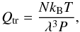 (1)where
 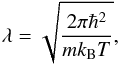 (2)and N is the number of particles, kB is the Boltzmann’s constant, P is the pressure, and m the mass of the particle. The rest of this section considers the internal part, Qint.
2.2. Vibrational energies
The energy levels of the harmonic oscillator (HO) 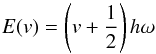 (3)depend on the integer vibrational quantum number v = 0,1,2,... These energy levels are equally spaced by
  (4)The frequency
  depends on the constant k, which is the force constant of the oscillator, and μ, the reduced mass of the molecule. The lowest vibrational level is
  . The harmonic oscillator potential approximates a real diatomic molecule potential well enough in the vicinity of the potential minimum at R = Re, where R is the internuclear distance and Re is the equilibrium bond distance, but it deviates increasingly for larger | R−Re |. A better approximation is a Morse potential,
 ![Mathematical equation: \begin{equation} E_{\rm pot}(R) = E_{\rm D}\left[1-{\rm e}^{-a(R-R_{\rm e})}\right]^2, \end{equation}](/articles/aa/full_html/2016/11/aa27209-15/aa27209-15-eq24.png) (5)where ED is the dissociation energy of the rigid molecule. The experimentally determined dissociation energy
(5)where ED is the dissociation energy of the rigid molecule. The experimentally determined dissociation energy  , where the molecule is dissociated from its lowest vibration level, has to be distinguished from the binding energy EB of the potential well, which is measured from the minimum of the potential. The difference is
  . The energy eigenvalues are
 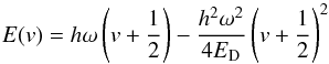 (6)with energy separations
 ![Mathematical equation: \begin{equation} \Delta E(v) = E(v+1)-E(v) = h\omega\left[1-\frac{h\omega}{2E_{\rm D}}(v+1)\right]. \label{eq:vibration_energy_separations} \end{equation}](/articles/aa/full_html/2016/11/aa27209-15/aa27209-15-eq30.png) (7)When using a Morse potential, the vibrational levels are clearly no longer equidistant: the separations between the adjacent levels decrease with increasing vibrational quantum number v, in agreement with experimental observations. In astrophysical applications these energies are commonly expressed in term-values G(v) = E(v) /hc, and the vibrational energies in the harmonic case are then given as
(7)When using a Morse potential, the vibrational levels are clearly no longer equidistant: the separations between the adjacent levels decrease with increasing vibrational quantum number v, in agreement with experimental observations. In astrophysical applications these energies are commonly expressed in term-values G(v) = E(v) /hc, and the vibrational energies in the harmonic case are then given as 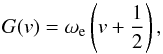 (8)and in the anharmonic case are given (when second-order truncation is assumed) as
 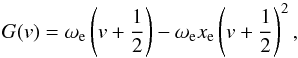 (9)where
  is the harmonic wave number,
 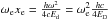 is the anharmonicity term, and
  is the vibrational frequency. We remark that literally, only ω is a frequency (measured in s-1), while ωe is a wave number (measured in cm-1), but in the literature ωe is commonly erroneously called a frequency any way. In the harmonic approximation, the Boltzmann factor (i.e. the relative population of the energy levels) can be summed analytically from v = 0 to v = ∞ Herzberg (1960),
 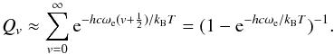 (10)
(10)
2.3. Rotational energies
In the rigid rotor approximation (RRA), a diatomic molecule can rotate around any axis through the centre of mass with an angular velocity ω∠. Its rotation energy is  (11)here I = μR2 is the moment of inertia of the molecule with respect to the rotational axis and | J | = Iω∠ is its rotational angular momentum. In the simplest quantum mechanical approximation, the square of the classical angular momentum is substituted by J(J + 1),
 and the rotational quantum number J can take only discrete values. The rotational energies of a molecule in its equilibrium position are therefore represented by a series of discrete values
  (12)and the energy separation between adjacent rotational levels
  (13)is increasing linearly with J. Rotational term-values are
  (14)where
  (15)is the main rotational molecular constant and F(J) is measured in the same units as G(v), that is, cm-1. A mathematical advantage (but physically erroneous) of Eq. (14) is that the rotational partition function Qrot can be calculated analytically,
  (16)A slightly more general approximation would be a non-rigid rotor. In this case, when the molecule rotates, the centrifugal force,
  , acts on the atoms and the internuclear distance widens to a value R that is longer than Re, and then the rotation energies are expressed as
  (17)where
  is the restoring force constant in a harmonic oscillator approximation, introduced above.
For a given value of the rotational quantum number J the centrifugal widening makes the moment of inertia larger and therefore the rotational energy lower, as expressed in Eq. (17). This effect compensates for the increase in potential energy. Using term-values, a centrifugal distortion constant De is introduced into Eq. (14), yielding  (18)It is often assumed that two terms are enough to have a good approximation and that more terms only give a negligible effect on the partition function. Unfortunately, this is rarely the case. When higher vibrational and rotational states are taken into consideration, as we show in the subsequent sections, higher order terms must be used. The rotational partition function Qrot can be computed in the same way as the vibrational partition function. However, there are 2J + 1 independent ways the rotational axis can orient itself in space with the same given energy. Furthermore, a symmetry factor, σ, has to be added as well if no full treatment of the nuclear spin degeneracy is included. In this case, oppositely oriented homonuclear molecules are indistinguishable, and half of their 2J + 1 states are absent. Hence σ is 2 for homonuclear molecules and unity for heteronuclear molecules, and this leads to half as many states in homonuclear molecules as in corresponding heteronuclear moleculs, such that Eq. (16)becomes
  (19)In the full spin-split degeneracy treatment for homonuclear molecules, the degeneracy factor is given by
  (20)for the possible orientations of the nuclear spins S1 and S2. For the two nuclei, each with spin S, there are S(2S + 1) antisymmetric spin states and (S + 1)(2S + 1) symmetric ones. For diatomic molecules, composed of identical Fermi nuclei1, the spin-split degeneracy for even and odd J states are
 ![Mathematical equation: \begin{equation} g_{n,{\rm even}}=[(2S+1)^2+(2S+1)]/2, \label{eq:spin} \end{equation}](/articles/aa/full_html/2016/11/aa27209-15/aa27209-15-eq72.png) (21)
(21)
![Mathematical equation: $$g_{n,{\rm odd}}=[(2S+1)^2-(2S+1)]/2,$$](/articles/aa/full_html/2016/11/aa27209-15/aa27209-15-eq73.png) respectively. The normalisation factor for gn is 1/(2S + 1)2. For identical Bose nuclei2, the spin-split degeneracy for even and odd J states are opposite to what they are for Fermi systems.
respectively. The normalisation factor for gn is 1/(2S + 1)2. For identical Bose nuclei2, the spin-split degeneracy for even and odd J states are opposite to what they are for Fermi systems.
2.4. Interaction between vibration and rotation
Interaction between vibrational and rotational motion can be allowed by using a different value of Bv for each vibrational level:  (22)where αe is the rotation-vibration interaction constant.
2.5. Electronic energies
The excited electronic energy levels typically are at much higher energies than the pure vibrational and rotational energy levels. For molecules they therefore contribute only a fraction to the partition function. Bohn & Wolf (1984) points out that for molecules the electronic state typically is non-degenerate because the electronic energy is typically higher than the dissociation energy, so that Qel = 1. Although this is the case for most molecules, others do have degenerate states, therefore Qel is sometimes fully calculated nonetheless. Naturally, molecules can and do occupy excited electronic states, as many experiments show. The electronic partition function is expressed as  (23)where
  is the electronic statistical weight, where δi,j is the Kronecker delta symbol, which is 1 if Λ = 0 and 0 otherwise.
2.6. Vibrational and rotational energy cut-offs and the basic concept of quantum numbers
If the semi-classical approach to the very high eigenstates (where this approximation has already lost its validity) is maintained by assigning v and J quantum numbers either as reached from the Morse potential (Eq. (7)) or from introducing second-order terms (as is most common), then the absurdity in the approach becomes more and more obvious. In Herzberg’s pragmatic interpretation (Herzberg 1950, p. 99–102) the classical theory is applied until the dissociation energy is reached (which for H2 corresponds to v = 14), and then v values are disregarded above this. Other authors have not always been happy with this interpretation, however, and insisted on including v values well above the dissociation energy to a somewhat arbitrary maximum level, which affects the value of the partition function substantially at high temperatures. In the Morse potential (Eq. (7)) the vibrational eigenstates can in principle be counted up to v quantum numbers corresponding to approximately twice the dissociation energy, and for even higher v quantum numbers, the vibrational energy becomes a decreasing function of the increasing v number: ![Mathematical equation: \begin{equation} \Delta E(v) = h\omega\left[1- \frac{h\omega}{2E_{\rm D}}(v+1)\right] < 0, \end{equation}](/articles/aa/full_html/2016/11/aa27209-15/aa27209-15-eq86.png) (24)solving for v where ΔE(v) first becomes lower than or equal to 0, we obtain
(24)solving for v where ΔE(v) first becomes lower than or equal to 0, we obtain  (25)The next level, vmax + 1, would produce zero or even negative energy addition. To solve this failure, more terms are needed to better approximate the real potential. Expressing vmax in vibrational term molecular constants, we obtain
  (26)vmax is sometimes used as a cut-off level for summation of vibrational energies (e.g. Eq. (25)).
The classical non-rigid rotor approximation, Eq. (18)also shows that the energy between adjacent levels decreases with increasing J, thus writing Eq. (18)for J and J + 1 states and making the difference between eigenstates equal to zero,  (27)and solving for J, we obtain the maximum rotational number,
  (28)The summation over rotational energies is commonly cut-off at some arbitrary rotational level or is approximated by an integral from 0 to ∞. When examining the literature, we did not note this Jmax expression. As with the non-harmonic oscillator, adding more terms to the non-rigid rotor approximation would give a better approximation. Now it is possible to measure more terms (ωyey,ωzez, ... for vibrational levels, He for rotational levels). Although they are important for high-temperature molecular line lists and partition functions, they are often calculated only from energy levels measured in the vicinity of the bottom of the potential well. For higher v and J values, the resulting energies can therefore still deviate from experimentally determined energy term values. Furthermore, the whole concept of quantum numbers v and J and associated degeneracies etc. of course relates to the classical approximations in quantum theory, which breaks down at energies far from the validity of a description of the molecule as a rotating system of some kind of isolated atoms bound to one another by some kind of virtual spring. This shows that there is an unclear limit beyond which it is no longer meaningful to continue adding higher order terms to expand the simple quantum number concept to fit the highest measured energy levels. At these highest levels there is nothing other than the mathematical wavefunction itself that represent reality in a meaningful way.
Given these limitations in defining the uppermost levels in a meaningful way within the semi-classical quantum mechanics, the question is whether in the end it is not more accurate to use only experimental energy levels in the construction of the partition function. However, exactly for the uppermost levels there is no such concept as experimentally determined energy levels summed to a partition function. The first problem is the practical one that for no molecule all the levels have been measured. For any missing level an assumption has to be applied, which could be to exclude the level in the summation, to make a linear fit of its energy between the surrounding measured energy levels, or to construct some type of polynomial fit from which to determine the missing levels, which would then be based on a choice of harmonic or anharmonic and rigid or non-rigid rotor or other polynomial fits. Another practical limitation is that experimentally, energy levels beyond the molecular dissociation energy would be seen. These levels can either give rise to a photo-dissociation of the molecule or relax back into a bound state, each with a certain probability. To construct a meaningful partition function, it would therefore at best have to be both temperature and pressure dependent, taking into account the timescales for molecular dissociation and recombination. An even more fundamental problem in defining a partition function based on experimental data is that each observed energy level has to be “named”. This naming is done by assigning a quantum number, which associates the measurements to a chosen semi-classical theory, however, and the quantum numbers associated with the state determines the degeneracy that the summation in the partition function will be multiplied with. This dilemma becomes perhaps more clear for slightly larger molecules than H2 where the degeneracy of the bending mode is multiplied directly into the partition function, but is a non-trivial function of the assigned vibrational quantum number of the state (Sørensen & Jørgensen 1993), while at the same time quantum mechanical ab initio calculations show that the wavefunction of the uppermost states can only be expressed as a superposition of several wavefunctions that are expressed by each their set of quantum numbers (Jørgensen et al. 1985), such that there is no “correct” assignment of the degeneracy factor that goes into the “experimental” partition function. There have been various ways in the literature to circumvent this problem. The most common is to ignore it. In some cases (e.g. Irwin 1987; Kurucz, priv. comm.) it was chosen to first complement the “experimental” values with interpolation between the measured values and then add extrapolated values above the dissociation energy (ignoring the pressure dependence) based on polynomial fits to the lower levels, with a cut-off of the added levels determined by where the order of the fit caused energy increments of further states to become negative (determined e.g. from Eqs. (25)and (28)). For low temperatures these inconsistencies have no practical implication because the somewhat arbitrarily added eigenstates do not contribute to the final partition function within the noise level. For higher temperatures, however, the uncertainty due to the inconsistency of how to add energy levels above the dissociation energy becomes larger than the uncertainty in using a polynomial fit, rather than the actually computed values, as illustrated in Fig. 1. Realising that strictly speaking there is no such concept as an experimentally summed partition function, and there is no “correct” upper level, we decided for a hybrid model, where the uppermost energy level in our summations are the minimum of the last level before the dissociation energy and the level where the energy increments become negative according to Eqs. (38)and (39), see case 8 in the next section for more details. For high temperatures this approach will give results in between the results that would be obtained by a cut at the dissociation energy of the ground electronic state and an upper level determined by Eqs. (38)and (39), or a more experimentally inspired upper level (black curve), as is illustrated in Fig. 1. The difference between the three methods (upper cuts) is an illustration of the unavoidable uncertainty in the way the partition functions can be calculated today. In the future, computers may be powerful enough to make sufficiently accurate ab initio calculations of these uppermost energy levels (but today the upper part of the ab initio energy surface is most often fitted to the experiments rather than representing numerical results).
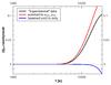 |
Fig. 1 Difference between different methods used to stop the summation (upper cuts) of the partition function. Different cut-offs are compared to the partition function obtained from case 8 (see text for more details), which is the zero line. The curve marked “experimental” data is derived by summing the Boltzmann factor of experimental data for the ground state used in Kurucz (priv. comm.)3. The blue curve is is the summation for the ground electronic state summed to D0 only. The red curve is the corresponding summation of energy levels of the three lowest electronic states based on Dunham coefficients and with a cut-off according to Eqs. (38) and (39). |
There are no restrictions on the number of energy eigenstates available for an isolated molecule before dissociation. However, the physical conditions of a thermodynamic system impose restrictions on the number of possible energy levels through the mean internal energy (Cardona & Crivellari 2005; Vardya 1965). A molecule in a thermodynamic system is subjected to the interaction with other molecules through collisions and with the background energy that permeates the system, making the number of energy states available dependent on the physical conditions of the system. From a geometric point of view, in a thermodynamic system with total number density of particles N, the volume occupied by each molecule considering that the volume is cubic and of side L, is L3 = 1 /N. This imposes a maximum size that the molecule may have without invading the space of other molecules, and therefore the number of states becomes finite. From a physical point of view, the number of energy states of the molecules is delimited by the interactions with the rest of the system since the energy state above the last one becomes dissociated by the mean background thermal energy of the system under study. Hence the maximum number of states available for a particle is dependent on the properties of the surrounding system. Cardona & Corona-Galindo (2012) have shown that in a dense medium (N ≥ 1021 cm-3) interaction between molecules and their surroundings starts to become important and that the physical approach dominates the geometrical one. They also derived equations for the maximum vibrational and rotational levels in such conditions, assuming the rigid rotor approximation.
3. Simplifications used in other studies
In this section we briefly review the simplifications in calculating Qint that have been used and how they compare to each other.
3.1. Case 1
This is the simplest case that is often given in textbooks: a simple product of harmonic oscillator approximation (HOA) and rigid rotor approximation (RRA), respectively summed and integrated to infinity, assuming Born-Oppenheimer approximation without interaction between vibration and rotation, and assuming that only the ground electronic state is present. Qint then becomes a simple product of Eqs. (10)and (26):  (29)where c2 = hc/kB is the second radiation constant.
3.2. Case 2
This time, HOA is dropped. vmax is evaluated by Eq. (25)4, only ground electronic state and no upper energy limit are assumed: ![Mathematical equation: \begin{eqnarray} Q_{\rm int} &=& {\rm exp}\left[\frac{c_2}{T}\left(\frac{\omega_{\rm e,1}}{2}-\frac{\omega_{\rm e}x_{\rm e,1}}{4}\right)\right]\nonumber\\ &&\quad \times \frac{T}{\sigma c_2B_{\rm e}}\sum_{v=0}^{v_{\rm max}}{\rm exp}\left[\frac{c_2}{T}\omega_{\rm e}\left(v+\frac{1}{2}\right)-\omega_{\rm e}x_{\rm e}\left(v+\frac{1}{2}\right)^2\right], \label{eq:case2} \end{eqnarray}](/articles/aa/full_html/2016/11/aa27209-15/aa27209-15-eq106.png) (30)where the first term refers to the lowest vibrational level of the ground state instead of the bottom of the potential well.
(30)where the first term refers to the lowest vibrational level of the ground state instead of the bottom of the potential well.
3.3. Case 3
This is the same as case 2, but this time Be in Eq. (30) is replaced by Bv, obtained by Eq. (22)(i.e. the Born-Oppenheimer approximation is abandoned): ![Mathematical equation: \begin{eqnarray} Q_{\rm int} &=& {\rm exp}\left[\frac{c_2}{T}\left(\frac{\omega_{\rm e,1}}{2}-\frac{\omega_{\rm e}x_{\rm e,1}}{4}\right)\right]\nonumber\\ &&\quad\times\sum_{v=0}^{v_{\rm max}}\frac{T}{\sigma c_2B_{v}}{\rm exp}\left[\frac{c_2}{T}\omega_{\rm e}\left(v+\frac{1}{2}\right)-\omega_{\rm e}x_{\rm e}\left(v+\frac{1}{2}\right)^2\right]\cdot \label{eq:case3} \end{eqnarray}](/articles/aa/full_html/2016/11/aa27209-15/aa27209-15-eq108.png) (31)
(31)
3.4. Case 4
This is the same as case 3, but this time an arbitrary energy truncation for the vibrational energy is added. The most commonly used (Tatum 1966; Sauval & Tatum 1984; Rossi et al. 1985; Gamache et al. 1990; Goorvitch 1994; Gamache et al. 2000; Fischer et al. 2003) value is 40 000 cm-1: ![Mathematical equation: \begin{eqnarray} Q_{\rm int} &=& {\rm exp}\left[\frac{c_2}{T}\left(\frac{\omega_{\rm e,1}}{2}-\frac{\omega_{\rm e}x_{\rm e,1}}{4}\right)\right]\nonumber\\ &&\quad\times\sum_{v=0}^{v_{\rm max}=40\,000 ~{\rm cm}^{-1}}\!\!\frac{T}{\sigma c_2B_{v}}{\rm exp}\left[\frac{c_2}{T}\omega_{\rm e}\left(v+\frac{1}{2}\right)\!-\!\omega_{\rm e}x_{\rm e}\left(v+\frac{1}{2}\right)^2\right]\cdot \label{eq:case4} \end{eqnarray}](/articles/aa/full_html/2016/11/aa27209-15/aa27209-15-eq110.png) (32)
(32)
3.5. Case 5
In this case, excited electronic states are added, ![Mathematical equation: \begin{eqnarray} Q_{\rm int}& =& {\rm exp}\left[\frac{c_2}{T}\left(\frac{\omega_{\rm e,1}}{2}-\frac{\omega_{\rm e}x_{\rm e,1}}{4}\right)\right] \nonumber\\ &&\quad\times \sum_{\rm e}^{T_{\rm e,max}}\sum_{v=0}^{\nu_{\rm max}}\frac{\tilde{\omega_{\rm e}}T}{\sigma c_2B_{v}}{\rm exp}\!\left[\frac{c_2}{T}\omega_{\rm e}\left(v+\frac{1}{2}\right)\!-\!\omega_{\rm e}x_{\rm e}\left(v+\frac{1}{2}\right)^2\!\!+T_{\rm e}\!\right], \label{eq:case5} \end{eqnarray}](/articles/aa/full_html/2016/11/aa27209-15/aa27209-15-eq111.png) (33)where Te,max = 40 000 cm-1.
(33)where Te,max = 40 000 cm-1.
3.6. Case 6
This case provides the full treatment: we finally drop the RRA. As in cases 3–5, this case also fully abandons the Born-Oppenheimer approximation because electronic and vibrational and rotational states are interacting and depend on one another. Different vibrational and rotational molecular constants are used for the different electronic levels. Furthermore, the arbitrary truncation is dropped and the real molecular dissociation energy, D0, is used for the ground state. In principle, molecules can occupy eigenstates above the dissociation energy, but they are not stable and dissociate almost instantly or relax to lower states below the dissociation level. Since the timescale for dissociation is usually shorter than for relaxation, molecules tend to dissociate rather than relax. Furthermore, a pre-dissociation state is usually present for molecules, where no eigenstates can be distinguished and a continuum of energies is present. This regime is beyond the scope of this work. For excited electronic states the ionisation energy is used instead of the dissociation energy. The equation for the full treatment takes the form ![Mathematical equation: \begin{eqnarray} Q_{\rm int} &=& {\rm exp}\left[\frac{c_2}{T}\left(\frac{\omega_{\rm e,1}}{2}-\frac{\omega_{\rm e}x_{\rm e,1}}{4}\right)\right] \nonumber\\ &&\quad\times\sum_{e=0}^{T_{\rm e,max}} \sum_{v=0}^{v_{\rm max}}\sum_{J=0}^{J_{\rm max}} \tilde{\omega_{\rm e}}(2J+1){\rm exp}\left[\frac{-c_2}{T}(T_{\rm e}+G_{v}+F_J)\right], \label{eq:case6} \end{eqnarray}](/articles/aa/full_html/2016/11/aa27209-15/aa27209-15-eq113.png) (34)where Gv is calculated as in Eq. (9), FJ = BvJ(J + 1)−DνJ2(J + 1)2, where Bv is calculated as in Eq. (22), and
(34)where Gv is calculated as in Eq. (9), FJ = BvJ(J + 1)−DνJ2(J + 1)2, where Bv is calculated as in Eq. (22), and  . Te,max is the term energy of the highest excited electronic state and is taken into account. For each electronic state the v and J quantum numbers are summed to a maximum value that corresponds to the dissociation energy of that particular electronic state.
3.7. Case 7
For homonuclear molecules, nuclear spin-split degeneracy must also be taken into account. In this case, the form of the equation is ![Mathematical equation: \begin{eqnarray} Q_{\rm int} &=& {\rm exp}\left[\frac{c_2}{T}\left(\frac{\omega_{\rm e,1}}{2}-\frac{\omega_{\rm e}x_{\rm e,1}}{4}\right)\right]\nonumber \\ &&\quad\times\sum_{e=0}^{{e}_{\rm max}} \sum_{v=0}^{v_{\rm max}}\sum_{J=0}^{J_{\rm max}} \tilde{\omega_{\rm e}}g_n(2J+1){\rm exp}\left[\frac{-c_2}{T}(T_{\rm e}+G_{v}+F_J)\right], \label{eq:case7} \end{eqnarray}](/articles/aa/full_html/2016/11/aa27209-15/aa27209-15-eq118.png) (35)where gn is calculated as in Eq. (21).
(35)where gn is calculated as in Eq. (21).
3.8. Case 8
This is the most accurate model we present here. Although cases 6 and 7 give reasonable results, they are still not sufficient at high temperatures. Molecular constants are conceptually rooted in classical mechanics (such as force constants of a spring and centrifugal distortion), and most often they are evaluated only from lower parts of the potential well and represent higher states poorly. For this reason it is more accurate to use a Dunham polynomial (1932) to evaluate energy levels,  (36)where Yik are Dunham polynomial fitting constants. These constants are not exactly related to classical mechanical concepts, such as bond lengths and force constants, and as such represent one step further into modern quantum mechanics. The lower order constants have values very close to the corresponding classical mechanics analogue constants used in cases 1–7, with the largest deviations occurring for H2 and hydrides (Herzberg 1950, p. 109). For example, the differences between the molecular constants of H2X 1sσ state (taken from Pagano et al. 2009) and the corresponding Dunham coefficients, obtained in this work, are 0.12% for ωe and Y10, 3% for ωexe and Y20, 72% for ωeye and Y30, 0.015% for Be and Y01, 1.8% for αe and Y11, 5.9% for γe and Y21, 0.25% for De and Y02, 40% for βe and Y12, etc. Dunham polynomial constants used together as a whole represent all experimental data more accurate than the classical picture in cases 1–75. Results from Eq. (36)are then summed to obtain Qint:
 ![Mathematical equation: \begin{eqnarray} Q_{\rm int}&= &\sum_{{\rm e},v,J}^{{e}_{\rm max},v_{\rm max},J_{\rm max}}\omega_{\rm e}(2J+1)\frac{1}{8}[(2S+1)^2 \nonumber\\ &&\quad -(-1)^J(2S+1)]{\rm exp}\left[\frac{-c_2}{T}T_{\rm Dun}\right]. \label{eq:case8} \end{eqnarray}](/articles/aa/full_html/2016/11/aa27209-15/aa27209-15-eq135.png) (37)In this case, vmax and Jmax are evaluated numerically, defined as the first v or J, where ΔE ≤ 0 (as in case 2, but now based on less biased coefficients), with ΔE given as
(37)In this case, vmax and Jmax are evaluated numerically, defined as the first v or J, where ΔE ≤ 0 (as in case 2, but now based on less biased coefficients), with ΔE given as ![Mathematical equation: \begin{equation} \Delta E(v) = \sum_{i=1}^{i_{\rm max}}Y_{i,0}\left[\left(v+\frac{3}{2}\right)^i-\left(v+\frac{1}{2}\right)^i\right] \leq 0, \label{eq:mine_vMax} \end{equation}](/articles/aa/full_html/2016/11/aa27209-15/aa27209-15-eq138.png) (38)for vmax, and
(38)for vmax, and ![Mathematical equation: \begin{equation} \Delta E(J) = \sum_{i=0,k=1}^{i_{\rm max},k_{\rm max}}Y_{i,k}\left({v}+\frac{1}{2}\right)^i\left[(J+1)^k(J+2)^k-J^k(J+1)^k\right] \leq 0 \label{eq:mine_Jmax} \end{equation}](/articles/aa/full_html/2016/11/aa27209-15/aa27209-15-eq140.png) (39)for Jmax.
(39)for Jmax.
4. Thermodynamic properties
From Qtot and its first and second derivatives we calculate thermodynamic properties. For Qtr (Eq. (1)) we assume 1 mol of ideal-gas molecules, N = NA, the Avogadro’s number. The ideal-gas standard-state pressure (SSP) is taken to be p° = 1 bar and the molecular mass is given in amu. The internal contribution Eint to the thermodynamic energy, the internal energy U−H(0), the enthalpy H−H(0), the entropy S, the constant-pressure specific heat Cp, the constant-volume specific heat Cv, the Gibbs free energy G−H(0), and the adiabatic index γ are obtained respectively from ![Mathematical equation: \begin{eqnarray} &&E_{\rm int} = RT^2\frac{\partial {\rm ln}Q_{\rm int}}{\partial T} \\ &&U-H(0)= E_{\rm int}+\frac{3}{2}RT \\ && H-H(0)= E_{\rm int}+\frac{5}{2}RT \\ && S = R~ {\rm ln}Q_{\rm tot} + \frac{RT}{Q_{\rm tot}}\left( \frac{\partial Q_{\rm tot}}{\partial T} \right) \\ && C_{\rm p}=R\left[2T \left(\frac{\partial {\rm ln}Q_{\rm int}}{\partial T}\right)+T^2\left(\frac{\partial^2 {\rm ln} Q_{\rm int}}{\partial T^2}\right)\right]+\frac{5}{2}R \\ && C_v=\frac{\partial E_{\rm int}}{\partial T} +\frac{3}{2}R \\ && G-H(0) = -RT~{\rm ln}Q_{\rm tot}+RT \\ && \gamma=\frac{H-H(0)}{U-H(0)}\cdot \end{eqnarray}](/articles/aa/full_html/2016/11/aa27209-15/aa27209-15-eq152.png)
5. Orto/para ratio of molecular hydrogen
In addition to equilibrium hydrogen, we also calculate the normal hydrogen following the paradigm of Colonna et al. (2012). In this case, ortho-hydrogen and para-hydrogen are not in equilibrium, but act as separate species. This aspect is particularly important for simulations of protoplanetary disks. The equilibrium timescale is short enough (300 yr) that the ortho/para ratio (OPR) can thermalise in the lifetime of a disk, but the equilibrium timescale is longer than the dynamical timescale inside about 40 AU Boley et al. (2007). In case of normal hydrogen, ortho and para states have to be treated separately. Then Eq. (37)is split into two, one for para states: ![Mathematical equation: \begin{equation} Q_{\rm para}=\sum_{{\rm e},v,J_{\rm even}}^{{\rm e}_{\rm max},v_{\rm max},J_{\rm max}}\omega_{\rm e}(2J+1){\rm exp}\left[\frac{-c_2}{T}T_{\rm Dun}\right], \label{eq:normalH2_para} \end{equation}](/articles/aa/full_html/2016/11/aa27209-15/aa27209-15-eq153.png) (48)and one for orhto states:
(48)and one for orhto states: ![Mathematical equation: \begin{equation} Q_{\rm ortho}=\sum_{{\rm e},v,J_{\rm odd}}^{{\rm e}_{\rm max},v_{\rm max},J_{\rm max}}\omega_{\rm e}(2J+1){\rm exp}\left[\frac{-c_2}{T}(T_{\rm Dun}-\varepsilon_{001})\right]. \label{eq:normalH2_ortho} \end{equation}](/articles/aa/full_html/2016/11/aa27209-15/aa27209-15-eq154.png) (49)We note that weights for nuclear spin-split are omitted. The partition function for ortho-hydrogen is (as opposed to Qpara) referred to the first excited rotational level (J = 1) of the ground electronic state in its ground vibrational level. ε001 can be considered as the formation energy of the ortho-hydrogen Colonna et al. (2012). Qint is then Colonna et al. (2012)
(49)We note that weights for nuclear spin-split are omitted. The partition function for ortho-hydrogen is (as opposed to Qpara) referred to the first excited rotational level (J = 1) of the ground electronic state in its ground vibrational level. ε001 can be considered as the formation energy of the ortho-hydrogen Colonna et al. (2012). Qint is then Colonna et al. (2012)  (50)where gp and go are the statistical weights of the ortho and para configurations, 0.25 and 0.75, respectively. Moreover, the OPR is not necessarily either 3 or in equilibrium, but can be a time-dependant variable. The last consideration is beyond the scope of this work, therefore we do not discuss different ratios and assume that there are only two possibilities: either H2 is in equilibrium or not.
6. Results and comparison
We finally are ready to compare these different approaches. We here focus on H2, but we plan to apply the theory given above to other molecules in a forthcoming paper. Since Qint varies with several orders of magnitude as a function of temperature, we normalised the differences to case 8:  , where X is the case number.
Molecular constants for cases 1–7 were taken from the NIST6 database, summarised in Pagano et al. (2009). D0 = 36 118.0696 cm-1 Piszczatowski et al. (2009). Experimental and theoretical data for molecular hydrogen for case 8 was taken from a number of sources that are summarised in Table 1. Theoretical calculations were used only when observational data were incomplete. For every electronic state, coefficients were fitted to all v−J configurations simultaneously using a weighted Levenberg-Marquardt Transtrum & Sethna (2012) algorithm and giving lower weights to theoretical data.
Summary of data sources for H2 energy levels.
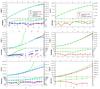 |
Fig. 2 Energy levels for the X 1sσ and D 3pπ states of H2. Top left: X 1sσ vibrational energies. Top right: D 3pπ vibrational energies. Middle left: X 1sσ (v = 0) energy levels. Middle right: D 3pπ (v = 0) energy levels. Bottom left: X 1sσ (v = 10) energy levels. Bottom right: D 3pπ (v = 10) energy levels. See text for more details. |
6.1. Determination of Dunham coefficients and evaluation of their accuracy
In this subsection we show how estimated energies from our Dunham coefficients for particular e,v,J configurations compare to those estimated from molecular constants and to experimental data. For simplicity we will here discuss only two electronic (X 1sσ, D 3pπ)7 and vibrational (v = 0 and 10) configurations of molecular hydrogen. Additionally, for the X 1sσ state we show Dunham coefficients from Dabrowski (1984) and Irwin (1987). For Dabrowski (1984) signs had to be inverted for the Y02, Y04, Y12, Y14, and Y22 coefficients so that they would correctly follow the convention presented in Eq. (36). The comparison is shown in Fig. 2. The top panels show vibrational energies of both states, middle panels show energy levels of the v = 0 vibrational state, and bottom panels show energy levels of the v = 10 vibrational state. Experimental data are shown as black dots, red curves represent calculations of this work, green curves calculations from molecular constants, blue and cyan calculations using Dunham coefficients from Irwin (1987) and Dabrowski (1984), respectively. The top panels in all panels show the resulting energies, the bottom panels the residuals (calculated – experimental) in logarithmic scale. Triangles, facing down, indicate that the calculated energy is lower than observed, upward facing triangles that it is higher. These figures show that energies calculated from molecular constants can diverge substantially, especially in the X 1sσ state, which contributes most to Qint. For most of the states the results of Irwin (1987) are of similar quality as ours (but we used fewer coefficients, which speeds up the Qint calculation), while for the lower vibrational levels of the X 1sσ state our results are much more accurate (especially at high J). A complete set of Dunham coefficients is given in Tables A.1 to A.22. The number of coefficients for all cases was chosen separately from examining the RMSE (root mean square error, compared to experimental/theoretical data) to determine those with the lowest number of coefficients and lowest RMSE. In some cases as little as a 5 × 5 matrix is enough (e.g. EF 2pσ2pσ2), whereas in other cases up to a 11 × 11 matrix is needed. These differences depend on the complexity of the shape of the potential well. In all the tables the limiting energies are given up to which particular matrices should be used. All the limitations have to be employed (maximum energy as well as Eqs. (38)and (39)) for every electronic configuration, since all the coefficients are only valid under these limitations.
6.2. Comparison of cases 1 to 8
First, we consider only the equilibrium H2. The comparison of cases 1–7 to case 8 is shown in Fig. (3). The main differences between all cases come from whether or not rigid-rotor approximation is used. The simplest case, case 1, underestimates Qint throughout the complete temperature range. The underestimation in the high-temperature range is easily explained by the equidistant separation (or linear increase with increasing J) between eigenstates (Eqs. (4)and (13), respectively): in HOA/RRA the eigenstate energies are higher for a given set of v, J values than when less strict approximations are used (Eq. (7)). This effect is particularly strong for H2, since the rotational distortion constant De (see Eq. (18)) is so large (De,H2 = 0.0471 for the X1Σg state, whereas it is only De,CO = 6.1215 × 10⁻⁶ in the case of CO). The higher energy levels are therefore less populated in the HOA/RRA than in a more realistic computation, and these levels play a relatively larger role the higher the temperature. At the lowest temperatures the few lowest eigenstates dominate the value of Qint, and these levels have slightly too high energies in HOA/RRA and therefore also cause Qint from HOA/RRA to be substantially underestimated for low temperatures. Numerical differences are small, but the percentage difference is substantial: between 80 K and 1200 K the difference is 10 to 20 percent. Anharmonicity (difference between cases 1 and 2) for H2 is only relevant above 1000 K. Interaction between rotation and vibration gives only 2 percent difference (between cases 2 and 3) below 2000 K and becomes substantial thereafter. Since D0 = 36118.0696 cm-1, and Te = 91 700 cm-1 for the  state, for H2 it makes no difference whether excited electronic states are taken into account or not for low temperatures or if arbitrary truncation (e.g. 40 000 cm-1) is below the first excited state. On the other hand, summing above the dissociation energy, at temperatures above 10 000 K gives larger Qint than it should be, assuming only the ground electronic state is available. On the other hand, if the RRA is used, Qint is still somewhat too low even if erroneously, it is summed to infinity. Case 6 shows how large the difference is when nuclear spin-split degeneracy is omitted from the full calculations and σ = 1/2 is used.
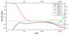 |
Fig. 3 Comparison of different approaches for calculating Qint for the H2 molecule. Case 1 is identical to case 2 below 1500 K; case 4 is completely identical to case 5 for H2. All of the methods (i.e. cases 1–7) diverge substantially from our most accurate computation (case 8) for low as well as high temperatures. |
For temperatures below 200 K, case 6 overestimates the partition function by up to a factor of 2 compared to case 8. For T between 200 K and 2000 K, cases 6 and 7 are indistinguishable from case 8. Above 2000 K even case 7 (and 6) gives different results. The latter is due to poor predictions of the higher rotational energy states at higher vibrational levels.
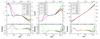 |
Fig. 4 Adiabatic index (left panel), normalised internal energy (middle panel), and entropy (right panel) for the H2 molecule. In the left panel we also show the constants γ = 5/3 and γ = 7/5 . Residuals are for cases 1–7 with respect to case 8. In the left panel cases 1–5 are equal to γ = 7/5 below 1000 K, case 6 is identical to case 7 after 300 K, and case 7 is identical to case 8 until 6000 K; in the middle panel cases 1 to 5 are identical until 1000 K, and case 7 is almost identical to case 8 until 2000 K. |
Naturally, using different approaches (cases 1–8) leads to different estimates of thermodynamic quantities. In Fig. 4 the adiabatic index γ, the normalised internal energy (Eint/RT), and the entropy S are shown for all the cases. Constant adiabatic indexes (5/3 or 7/5) clearly completely misrepresent reality for a wide range of temperatures when local thermal equilibrium (LTE) is assumed. When considering the simplest cases (case 1 to 5), they follow the 7/5 simplification well until 1000 K, but are far from the most realistic estimate (case 8). Case 6 gives results almost identical to case 7 above 300 K. Case 7 is indistinguishable from case 8 up until 2000 K. The same trends can be seen for internal energy. From a first glance, the entropy seems to be very similar in all the cases, but this is because the dominating factor comes from Qtr. Keeping that in mind, variability throughout all the temperature range is substantial. Entropy in case 7 is accurate until 3000 K.
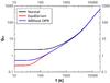 |
Fig. 5 Qint for equilibrium, normal, and one (i.e. neglecting OPR) hydrogen. |
Now we compare equilibrium and normal hydrogen. Equilibrium, normal, and one, neglecting OPR, partition functions are shown in Fig. 5. At low temperature, the three models show large differences, while in the high temperature range (T> 2000 K) the results coalesce. The same trends can be seen for the calculated thermodynamic quantities (Fig. 6). Both internal energy and specific heat at constant pressure are lower for normal hydrogen, whereas equilibrium hydrogen has higher values. The adiabatic index is dramatically different for both cases. Normal hydrogen does not have a depression at low temperatures. This depression can lead to accelerated gravitational instability and collapse in molecular clouds to form pre-stellar cores and protoplanetary cores in protoplanetary disks. Large differences in entropy are only present at temperatures below 300 K. Neglecting OPR would lead to intermediate values between normal and equilibrium hydrogen.
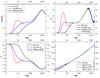 |
Fig. 6 Normalised internal energy, Cp, adiabatic index and entropy, calculated for equilibrium, normal, and with neglected OPR hydrogen. For Cp and entropy JANAF data are also shown. |
6.2.1. Other studies
There are a number of commonly used studies of Qint. Here we give a brief summary of how other studies were performed, which simplifications they used, which molecular constants were adopted, and for which temperature range they were recommended. We stress that although it is commonly done, data must not be extrapolated beyond the recommended values under any circumstances. The resulting partition functions as well as their derivatives often diverge from the true values remarkably fast outside the range of the data they are based on. In our present study we took care to validate our data and formulas, such that they can be used in a wider temperature range than thos of any previous study. Our data and formulas can be safely applied in the full temperature range from 1 K to 20 000 K and easily extended beyond 20 000 K in extreme cases, such as shocks, by use of the listed Dunham coefficients.
Tatum (1966, T1966)
presented partition functions and dissociation equilibrium constants for 14 diatomic molecules in the temperature range T = 1000–8000 K with 100 K steps. Calculations were made using case 5. The upper energy cut-off was chosen to be at 40 000 cm-1. Only the first few molecular constants were used (ωe,ωexe,Be,αe).
Irwin (1981, I1981)
presented partition function approximations for 344 atomic and molecular species, valid for the temperature range T = 1000–16 000 K. Data for molecular partition functions were taken from (Tatum 1966; McBride et al. 1963; Stull 1971). Irwin (1981) gave partition function data in the form of polynomials,  (51)which is very convenient to use. For each species, the coefficients of Eq. (51)were found by the method of least-squares fitting. Some molecular data were linearly extrapolated before fitting the coefficients. For the extrapolated data the weight was reduced by a factor of 106. Irwin stated that these least-squares fits have internally only small errors. However, a linear extrapolation to strongly non-linear data results in large errors even before fitting the polynomial, and the size of the errors due to this effect was not estimated.
Bohn & Wolf (1984, BW1984)
derived partition functions for H2 and CO that are valid for the temperature range T = 1000–6000 K. In principle, this paper aimed to show a new approximate way of calculating partition functions, specific heat cV, and internal energy Eint. Calculations were made using case 5 for “exact” partition functions and using assumptions of case 3 for approximations. Only the ground electronic state was included, and only the first few molecular constants were used (ωe,ωexe,Be,αe).
Sauval & Tatum (1984, ST1984)
presented total internal partition functions for 300 diatomic molecules, 69 neutral atoms, and 19 positive ions. Molecular constants (ωe,ωexe,Be,αe) were taken from Huber & Herzberg (1979). The partition function polynomial approximations are valid for the temperature range T = 1000−9000 K. The authors adopted the previously used equation, [T1966] (case 5) for all the species. A polynomial expression  (52)was used for both atoms and molecules. Here θ = 5040 /T.
Rossi et al. (1985, R1985)
presented total internal partition functions for 53 molecular species in the temperature range T = 1000–5000 K. Molecular constants (ωe,ωexe,Be,αe) were taken from Huber & Herzberg (1979). For diatomic molecules the authors followed Tatum’s Tatum (1966) paradigm, case 5. The authors claimed that QJ was evaluated with a non-rigid approximation Rossi et al. (1985), but upon a simple inspection it is clear that they used rigid-rotor approximation. They did, however, allow interaction between vibration and rotation. An arbitrary truncation in the summation over the electronic states is at 40 000 cm-1. For polynomial approximations the authors considered the “exact” specific heat, whose behaviour near the origin is more amenable to approximation schemes. The partition functions were then obtained by integration Rossi et al. (1985). Their specific heat approximation is  (53)where Z = T/ 1000 and am are coefficients. The partition function they obtained is listed as the seven filling constants a0 to a6 to the polynomial:
 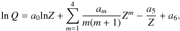 (54)
(54)
Kurucz (priv. comm., K1985)
commented on the situation regarding the partition functions of H2 and CO. Approximate expressions for the molecular partition functions in previous studies were considered not rigorous enough because they did not include coefficients of sufficiently high order and did not keep proper track of the number of bound levels. K1985 used experimentally determined energy levels, when available, and supplemented them with fitted values, presumably extended to a higher cut-off energy as discussed in Sect. 2.6 and Fig. 1 above. The author explicitly summed over the energies of the three lowest electronic states (data for H2 were derived from Dabrowski 1984) and gave polynomial fits for the partition functions between 1000 K and 9000 K and also tabulated the exact results with steps of 100 K.
Irwin (1987, I1987)
presented refined total internal partition functions for H2 and CO. The partition function polynomial approximations are valid for the temperature range T = 1000−9000 K. Estimated errors at 4000 K are 2% for H2 and 0.004% for CO. Yi,j for H2 were determined by using an equally weighted simultaneous least-squares fit of Dunham series using energy data obtained from Dabrowski (1984). This was done for the ground H2 electronic state only.
I1987 compared his results with those of (Kurucz, priv. comm.; Sauval & Tatum 1984) and found slightly higher values of Q, which he attributed to a combination of the number of included electronic states and a difference in the treatments of the highest rotational levels. Our results indicate that the main difference between the results of I1987 Irwin (1987) and K1985 Kurucz, priv. comm. is the use of slightly too low energies in I1987 of the highest rotational levels, and we conclude that the value trend by K1985 is slightly closer to the values obtained by a full treatment (our case 8) than are those of I1987. A main difference between our method and those of I1987, K1985, and older works is, however, that our method is applicable in a higher temperature range and can treat ortho and para states separately. It can therefore be used in a wider range of physical conditions, including shocks, non-equilibrium gasses, etc.
Pagano et al. (2009, P2009)
presented internal partition functions and thermodynamic properties of high-temperature (50–50 000 K) Jupiter-atmosphere species. The authors used case 7 to calculate the partition functions with more than the first few (e.g. ωe and ωexe, Be and De) molecular constants for the ground and first few electronically excited states. The calculations are completely self-consistent in terms of maximum rotational states for the individual vibrational levels, presumably such that E(v,Jmax) ≈ D0 for each v.
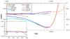 |
Fig. 7 Normalised Qint from other studies in their respective temperature ranges. Normalisation is made with respect to the results of this work, ((study – this work)/this work). C2012 is normalised to normal hydrogen, all other studies to equilibrium hydrogen. The inset shows the low-temperature range. |
Laraia et al. (2011, L2011)
presented total internal partition functions for a number of molecules and their isotopes for the temperature range 70–3000 K. The methods used in this study are based on (Gamache et al. 2000; Fischer et al. 2003). Rotational partition functions were determined using the formulae in (McDowell 1988; McDowell 1990). Vibrational partition functions were calculated using the harmonic oscillator approximation of Herzberg (1960). All state-dependent and state-independent degeneracy factors were taken into account in this study. The H2 partition function was calculated as a direct sum using ab initio energies. A four-point Lagrange interpolation was used for the temperature range with intervals of 25 K. Data are presented in an easily retrievable FORTRAN program Laraia et al. (2011).
Colonna et al. (2012, C2012)
gave a statistical thermodynamic description of H2 molecules in normal ortho/para mixture. The authors determined the internal partition function for normal hydrogen on a rigorous basis, solving the existing ambiguity in the definition of those quantities directly related to partition functions rather than on its derivatives Colonna et al. (2012). The authors used case 7 with more molecular constants for the ground and first few electronically excited states than shown with Eqs. (35). Internal partition function as well as thermodynamic properties for 5–10 000 K are also given.
Comparison.
Figure 7 shows the normalised value of Qint for molecular hydrogen from the ten different studies we have described here, in their respective temperature ranges listed in the respective studies. The normalisation is made with respect to the results of this work (case 8). For C2012 normal hydrogen Qint is used, whereas equilibrium hydrogen Qint is used for all the other studies. The main frame of Fig. 7 is for the 1000–20 000 K temperature range. The inset shows the low-temperature (10–1000 K) range. In the low-temperature range our results clearly differ only marginally from the three studies (P2009, L2011, C2012) that listed values of Qint for low temperatures (the percentage difference is smaller than 0.1 percent in most of the temperature range). Since L2011 did not normalise the spin-split degeneracy, their results had to be divided by a factor of 4 before the comparison, shown in Fig. 7. In the high-temperature range, all studies using cases 1–5 have large errors (also seen from our case comparison in Fig. 3). Since K1985 explicitly derived his partition functions from experimental energy data, his results are in very good agreement with our results (from case 8) for his given temperature range (1000–9000 K). I1987 is also in great agreement with both K1985 and our results for the same temperature range. Using the values of Yij determined by I1987 gives results that perfectly agree with our work, as expected. At the higher end of the I1987 recommended temperature range, however, the polynomial approximation starts to have larger errors (the estimated 2 percent). At the highest temperature range, P2009 and C2012 also start to show considerable errors. These two studies are the only ones based on summation of energy levels, calculated based on molecular constants, and the comparison of our work with P2009 and C2012 therefore illustrates approximately how large errors in Qint are obtained from methods based on molecular constants. The reason is, as mentioned before, that molecular constants are commonly fitted to the bottom of the potential well and poorly represent higher vibrational and rotational states energies. Finally, the I1981 results follow the T1966 results perfectly until 8000 K, which is the latter’s high temperature limit. Then, since I1981 extrapolated data, the corresponding Qint begin to show exponentially larger errors and is completely unreliable, which illustrates both how poor the HO + RR approximation represents reality (T1966 and I1981), and, in particular, how unreliable it can be to extrapolate beyond the calculated or measured data (as was done in the work of I1981), as seen clearly in Fig. 7.
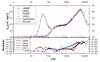 |
Fig. 8 Calculated Cp comparison to other studies. The top panel shows resulting Cp values, the bottom panel residuals (other – ours) on a logarithmic scale. Facing down triangles indicate that other results have lower values than ours, facing up triangles indicate that the values are higher. |
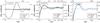 |
Fig. 10 Accuracies of polynomial fits for the partition functions of H2. |
Polynomial fit constants for partition functions of equilibrium, normal, and ortho and para H2.
In Fig. 8 our results for H2 specific heat at constant pressure are compared to (Stull 1971, JANAF), (30, Le Roy), (34, P2009) and (9, C2012). The latter is compared to our results for normal hydrogen, and the others are compared to our equilibrium hydrogen calculations. All calculations agree very well until 10 000 K. Figure 9 depicts our results for entropy calculations for H2. Once again, the agreement is very good (except with C2012 below 100 K), especially between our results and the JANAF data. However, there is a systematic offset between Le Roy and our results (and those of JANAF) of 11.52 J K-1 mol-1. This might be due to slightly different STP values, used by Le Roy et al. (1990), resulting in slightly different Qtr. We note that the JANAF data represent equilibrium H2, while we computed equilibrium as well as normal and ortho and para H2 (and span a much wider temperature range), which makes our data more generally applicable.
6.3. Polynomial fits
Following the common practice, we present polynomial fits to our results. All partition function data were fit to a fifth-order polynomial of the form  (55)The data for the partition function were spliced into three intervals to reach better accuracy. Polynomial constants are given in Table 2, and the fitting accuracy is shown in Fig. 10. Combining the three intervals, we reach an error smaller than 2 percent for all the temperature range. The decision for using lookup tables with significantly larger accuracy or the faster polynomial fits with increased errors needs to be made on an individual basis.
7. Conclusions
We have investigated the shortcomings of various simplifications that are used to calculate Qint and applied our analyses to calculate the time-independent partition function of normal, ortho and para, and equilibrium molecular hydrogen. We also calculated Eint/RT, H−H(0), S, Cp, Cv, −[G−H(0)] /T, and γ. Our calculated values of thermodynamic properties for ortho and para, equilibrium, and normal H2 are presented in Tables A.24, A.23, A.25, and A.26, rounded to three significant digits. Full datasets in 1 K temperature steps8 can be retrieved at http://astro.ku.dk/~hpg688/thermodynamic_data.html and at the CDS. The partition functions and thermodynamic data presented in this work are more accurate than previously available data from the literature and cover a more complete temperature range than any previous study in the literature. Determined Dunham coefficients for a number of electronic states of H2 are also reported. In future work we plan to use the method we described here to calculate partition functions and thermodynamic quantities for other astrophysically important molecular species as well.
S = 1/2, 3/2, 5/2, ...
S = 0, 1, 2, ...
Which has no physical meaning.
In most cases the estimated energies from Dunham polynomials differ by less than 1 cm-1 from experimentally determined energies. For high energies they can, however, sometimes differ by up to 20 cm-1.
K. P. Huber and G. Herzberg, “Constants of Diatomic Molecules” (data prepared by J. W. Gallagher and R. D. Johnson, III) in NIST Chemistry WebBook, NIST Standard Reference Database Number 69, eds. P. J. Linstrom and W. G. Mallard, National Institute of Standards and Technology, Gaithersburg MD, 20899, http://webbook.nist.gov, (retrieved July 19, 2014).
These states have a sufficiently large amount of molecular constants determined. Most other states have only few to no molecular constants determined, thus comparing them would be ungentlemanly.
Data with smaller temperature steps or beyond the given temperature range can be requested personally from the corresponding author.
Acknowledgments
We thank Åke Nordlund and Tommaso Grassi for a critical reading of this manuscript and all the very valuable discussions. We are also grateful to the referee, Robert Kurucz, for valuable comments and suggestions. AP work is supported by grant number 1323-00199A from the Danish Council for Independent Research (FNU).
References
- Abgrall, H., Roueff, E., Launay, F., Roncin, J. Y., & Subtil, J. L. 1993, J. Mol. Spectr., 157, 512 [NASA ADS] [CrossRef] [Google Scholar]
- Abgrall, H., Roueff, E., Launay, F., & Roncin, J.-Y. 1994, Can. J. Phys., 72, 856 [NASA ADS] [CrossRef] [Google Scholar]
- Bailly, D., Salumbides, E. J., Vervloet, M., & Ubachs, W. 2010, Mol. Phys., 108, 827 [NASA ADS] [CrossRef] [Google Scholar]
- Bohn, H. U., & Wolf, B. E. 1984, A&A, 130, 202 [NASA ADS] [Google Scholar]
- Boley, A. C., Hartquist, T. W., Durisen, R. H., & Michael, S. 2007, ApJ, 656, L89 [NASA ADS] [CrossRef] [Google Scholar]
- Born, M., & Oppenheimer, R. 1927, Ann. Phys., 389, 457 [Google Scholar]
- Cardona, O., & Corona-Galindo, M. G. 2012, Rev. Mex. Fis., 58, 174 [Google Scholar]
- Cardona, O., Simonneau, E., & Crivellari, L. 2005, Rev. Mex. Fis., 51, 476 [Google Scholar]
- Colonna, G., D’Angola, A., & Capitelli, M. 2012, Int. J. Hydrogen Energy, 37, 12, 9656 [CrossRef] [Google Scholar]
- Dabrowski, I. 1984, Can. J. Phys., 62, 1639 [NASA ADS] [CrossRef] [Google Scholar]
- Dunham, J. L. 1932, Phys. Rev., 41, 721 [NASA ADS] [CrossRef] [Google Scholar]
- Fischer, J., Gamache, R. R., Goldman, A., Rothman, L. S., & Perrin, A. 2003, J. Quant. Spec. Radiat. Transf., 82, 401 [Google Scholar]
- Gamache, R. R., Hawkins, R. L., & Rothman, L. S. 1990, J. Mol. Spectr., 142, 205 [NASA ADS] [CrossRef] [Google Scholar]
- Gamache, R. R., Kennedy, S., Hawkins, R. L., & Rothman, L. S. 2000, J. Mol. Struct., 517, 407 [Google Scholar]
- Glass-Maujean, M., Klumpp, S., Werner, L., Ehresmann, A., & Schmoranzer, H. 2007, J. Chem. Phys., 126, 144303 [NASA ADS] [CrossRef] [PubMed] [Google Scholar]
- Glass-Maujean, M., & Jungen, C. 2009, J. Phys. Chem. A, 113, 13124 [CrossRef] [Google Scholar]
- Glass-Maujean, M., Jungen, C., Schmoranzer, H., et al. 2013a, J. Mol. Spectr., 293, 19 [NASA ADS] [CrossRef] [Google Scholar]
- Glass-Maujean, M., Jungen, C., Spielfiedel, A., et al. 2013b, J. Mol. Spectr., 293, 1 [NASA ADS] [CrossRef] [Google Scholar]
- Glass-Maujean, M., Jungen, C., Schmoranzer, H., et al. 2013c, J. Mol. Spectr., 293, 11 [NASA ADS] [CrossRef] [Google Scholar]
- Goorvitch, D. 1994, ApJS, 95, 535 [NASA ADS] [CrossRef] [Google Scholar]
- Herzberg, G. 1950, Molecular Spectra and Molecular Structure, Vol. I: Spectra of Diatomic Molecules, 2nd edn (New York: Van Nostrand Reinhold) [Google Scholar]
- Herzberg, J. G. 1960, Molecular Spectra and Molecular Structure, Vol. II: Infrared and Raman Spectra of Polyatomic Molecules, 2nd edn. (New York: Van Nostrand Reinhold) [Google Scholar]
- Huber, K. P., & Herzberg, J. G. 1979, Molecular Spectra And Molecular Structure, Vol. IV. Constants of Diatomic Molecules (New York: Van Nostrand Reinhold) [Google Scholar]
- Irwin, A. W. 1981, ApJS, 45, 621 [NASA ADS] [CrossRef] [Google Scholar]
- Irwin, A. W. 1987, A&A, 182, 348 [NASA ADS] [Google Scholar]
- Jørgensen, U. G., Almlof, J., Gustafsson, B., Larsson, M., & Siegbahn, P. 1985, J. Chem. Phys., 83, 3034 [NASA ADS] [CrossRef] [Google Scholar]
- Laraia, A. L., Gamache, R. R., Lamouroux, J., Gordon, I. E., & Rothman, L. S. 2011, Icarus, 215, 391 [NASA ADS] [CrossRef] [Google Scholar]
- Le Roy, R., & Chapman, S. G., & McCourt, F. R. W. 1990, J. Phys. Chem., 94, 2 [CrossRef] [Google Scholar]
- McBride, B. J., Heimel, S., Ehlers, J. G., & Gordon, S. 1963, NASA SP, 3001, [Google Scholar]
- McDowell, R. S. 1988, J. Chem. Phys., 88, 356 [NASA ADS] [CrossRef] [Google Scholar]
- McDowell, R. S. 1990, J. Chem. Phys., 93, 2801 [NASA ADS] [CrossRef] [Google Scholar]
- Pagano, D., Casavola, A., Pietanza, L. D., et al. 2009, ESA Sci. Techn. Rev., 257 [Google Scholar]
- Piszczatowski, K., Łach, G., Przybytek, M., et al. 2009, J. Chem. Theory Comput., 5, 11 [Google Scholar]
- Ross, S. C., & Jungen, C. 1994, Phys. Rev. A, 50, 4618 [NASA ADS] [CrossRef] [Google Scholar]
- Rossi, S. C. F., Maciel, W. J., & Benevides-Soares, P. 1985, A&A, 148, 93 [NASA ADS] [Google Scholar]
- Sauval, A. J., & Tatum, J. B. 1984, ApJS, 56, 193 [NASA ADS] [CrossRef] [Google Scholar]
- Senn, P., & Dressler, K. 1987, J. Chem. Phys., 87, 6908 [NASA ADS] [CrossRef] [Google Scholar]
- Sørensen, G. O., & Jørgensen, U. G. 1993, J. Chem. Phys., 99, 3153 [NASA ADS] [CrossRef] [Google Scholar]
- Stull, D. R., & Prophet, H. 1971, JANAF Thermochemical, 2nd ed. (Washington: US Department of Commerce), NSRDS-NBS 37 [Google Scholar]
- Takezawa, S. 1970, J. Chem. Phys., 52, 2575 [NASA ADS] [CrossRef] [Google Scholar]
- Tatum, J. B. 1966, Publications of the Dominion Astrophysical Observatory Victoria, 13, 1 [Google Scholar]
- Transtrum, M. K., & Sethna, J. P. 2012, ArXiv e-print [arXiv:1201.5885] [Google Scholar]
- Vardya, M. S. 1965, MNRAS, 129, 345 [NASA ADS] [CrossRef] [Google Scholar]
- Wolniewicz, L., Orlikowski, T., & Staszewska, G. 2006, J. Mol. Spectr., 238, 118 [NASA ADS] [CrossRef] [Google Scholar]
- Yu, S., & Dressler, K. 1994, J. Chem. Phys., 101, 7692 [NASA ADS] [CrossRef] [Google Scholar]
Appendix A: Additional tables
Yi,j for X 1sσ state. Emax = ED = 36 118.0696.
Yi,j for B 2pσ state. Emax = 118 376.981.
Yi,j for C 2pπ state. Emax = 118 376.981.
Yi,j for EF 2pσ2pσ2 state, inner well. Emax = 105 000.0.
Yi,j for EF 2pσ2pσ2 state, outer well. Emax = 118 376.981.
Yi,j for B′ 3pσ state. Emax = 133 610.273.
Yi,j for D 3pπ state. Emax = 133 610.273.
Yi,j for GK 3dσ state, inner well. Emax = 116 900.0.
Yi,j for GK 3dσ state, outer well.
Yi,j for  state, inner well. Emax = 118 000.0.
Yi,j for state, outer well.
Yi,j for I 3dπ state.
Yi,j for J 3dδ state.
Yi,j for B”Bbar 4pσ state, inner well. Emax = 130 265.0.
Yi,j for B”Bbar 4pσ state, outer well. Emax = 138 941.911.
Yi,j for D′ 4pπ state. Emax = 138 941.911.
Yi,j for 5pσ state. Emax = 143 570.0.
Yi,j for 5pπ state. Emax = 143 570.0.
Yi,j for 6pσ state. Emax = 148 240.0.
Yi,j for 6pπ state. Emax = 148 240.0.
Yi,j for 7pσ state. Emax = 150 000.0.
Yi,j for 7pπ state. Emax = 150 000.0.
Thermodynamic properties of equilibrium H2.
Thermodynamic properties of normal H2.
Thermodynamic properties of ortho H2.
Thermodynamic properties of para H2.
All Tables
Polynomial fit constants for partition functions of equilibrium, normal, and ortho and para H2.
All Figures
|
Fig. 1 Difference between different methods used to stop the summation (upper cuts) of the partition function. Different cut-offs are compared to the partition function obtained from case 8 (see text for more details), which is the zero line. The curve marked “experimental” data is derived by summing the Boltzmann factor of experimental data for the ground state used in Kurucz (priv. comm.)3. The blue curve is is the summation for the ground electronic state summed to D0 only. The red curve is the corresponding summation of energy levels of the three lowest electronic states based on Dunham coefficients and with a cut-off according to Eqs. (38) and (39). |
| In the text | |
|
Fig. 2 Energy levels for the X 1sσ and D 3pπ states of H2. Top left: X 1sσ vibrational energies. Top right: D 3pπ vibrational energies. Middle left: X 1sσ (v = 0) energy levels. Middle right: D 3pπ (v = 0) energy levels. Bottom left: X 1sσ (v = 10) energy levels. Bottom right: D 3pπ (v = 10) energy levels. See text for more details. |
| In the text | |
|
Fig. 3 Comparison of different approaches for calculating Qint for the H2 molecule. Case 1 is identical to case 2 below 1500 K; case 4 is completely identical to case 5 for H2. All of the methods (i.e. cases 1–7) diverge substantially from our most accurate computation (case 8) for low as well as high temperatures. |
| In the text | |
|
Fig. 4 Adiabatic index (left panel), normalised internal energy (middle panel), and entropy (right panel) for the H2 molecule. In the left panel we also show the constants γ = 5/3 and γ = 7/5 . Residuals are for cases 1–7 with respect to case 8. In the left panel cases 1–5 are equal to γ = 7/5 below 1000 K, case 6 is identical to case 7 after 300 K, and case 7 is identical to case 8 until 6000 K; in the middle panel cases 1 to 5 are identical until 1000 K, and case 7 is almost identical to case 8 until 2000 K. |
| In the text | |
|
Fig. 5 Qint for equilibrium, normal, and one (i.e. neglecting OPR) hydrogen. |
| In the text | |
|
Fig. 6 Normalised internal energy, Cp, adiabatic index and entropy, calculated for equilibrium, normal, and with neglected OPR hydrogen. For Cp and entropy JANAF data are also shown. |
| In the text | |
|
Fig. 7 Normalised Qint from other studies in their respective temperature ranges. Normalisation is made with respect to the results of this work, ((study – this work)/this work). C2012 is normalised to normal hydrogen, all other studies to equilibrium hydrogen. The inset shows the low-temperature range. |
| In the text | |
|
Fig. 8 Calculated Cp comparison to other studies. The top panel shows resulting Cp values, the bottom panel residuals (other – ours) on a logarithmic scale. Facing down triangles indicate that other results have lower values than ours, facing up triangles indicate that the values are higher. |
| In the text | |
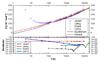 |
Fig. 9 Same as in Fig. 8, but for S. |
| In the text | |
|
Fig. 10 Accuracies of polynomial fits for the partition functions of H2. |
| In the text | |
Current usage metrics show cumulative count of Article Views (full-text article views including HTML views, PDF and ePub downloads, according to the available data) and Abstracts Views on Vision4Press platform.
Data correspond to usage on the plateform after 2015. The current usage metrics is available 48-96 hours after online publication and is updated daily on week days.
Initial download of the metrics may take a while.